1. Introduction
Liquid-metal flow is involved in many applications such as solar power generation (Deng, Jiang & Liu Reference Deng, Jiang and Liu2021), metallurgical processes (Davidson Reference Davidson1999) and the blanket of nuclear fusion reactors (Bühler Reference Bühler2007; Smolentsev et al. Reference Smolentsev, Moreau, Bühler and Mistrangelo2010). In the blanket flow, the fluid is generally subject to a driving pressure gradient, an external magnetic field and a heat flux through the wall, which combine to create a type of mixed convection problem. Studying the linear stability and nonlinear saturated states in this flow is of importance for the design of liquid-metal blankets for nuclear reactors, as the flow states determine the energy transport, wall-temperature and wall-stress fluctuations, which in the end affect the heat exchange rate of the reactor and structural integrity of the blanket wall under high temperature. These two aspects of the flow are the focuses of this work.
Blanket modules can have different orientations with respect to the magnetic field and gravity depending on the specific position and alignment of the module on the periphery of the fusion chamber. The actual geometry of the fluid channels inside a blanket can be complicated (Bühler Reference Bühler2007; Smolentsev et al. Reference Smolentsev, Moreau, Bühler and Mistrangelo2010; Chen et al. Reference Chen, Smolentsev and Ni2020, Reference Chen, Smolentsev and Ni2022; Wang et al. Reference Wang, Chen, Zhang and Ni2021; Zikanov et al. Reference Zikanov, Belyaev, Listratov, Frick, Razuvanov and Sviridov2021). However, simplified geometries and physical models have been frequently used to obtain quantitative and theoretical understanding of the flow phenomena, such as straight duct and pipe geometries with vertical or horizontal configuration. The vertical configuration includes downflow and upflow cases with side-wall heating or uniform heating, and the horizontal configuration includes bottom/top-wall heating or uniform heating. Different types of flow instability and saturated flow structures were identified in different cases, and systematic investigations of the problem in various cases are needed to better understand the magnetoconvection problem and optimise the blanket module design. The readers are referred to Zikanov et al. (Reference Zikanov, Belyaev, Listratov, Frick, Razuvanov and Sviridov2021) for a recent review on the current status and relevant studies. In the following, we will mainly discuss about the horizontal configuration with bottom heating for the reason that will be stated.
A magnetic field has been known to suppress three-dimensional (3-D) velocity fluctuations. Experiments in a horizontal pipe with a bottom heating showed that, although turbulence disappears and the flow relaminarises as the transverse magnetic field increases, with a further increased magnetic field, anomalous temperature fluctuations appeared in the turbulence-suppressing regime (Genin et al. Reference Genin, Zhilin, Ivochkin, Razuvanov, Belyaev, Listratov and Sviridov2011; Belyaev et al. Reference Belyaev, Ivochkin, Listratov, Razuvanov and Sviridov2015). The frequency/amplitude is much lower/higher than that of the turbulence in the weak-magnetic-field regime. Linear stability analysis of this problem has been carried out by Zikanov, Listratov & Sviridov (Reference Zikanov, Listratov and Sviridov2013) where a linear instability in the strong-magnetic-field regime is identified. The unstable modes exhibit large-scale roll-like structures that are aligned with the magnetic field. Their direct numerical simulations showed that the nonlinearly saturated flow structures are large-scale structures that bear similarities with the linearly unstable modes. Therefore, the authors proposed that the anomalous high-amplitude low-frequency temperature fluctuations are attributed to this linear instability and hypothesised the flow structure to be of a natural convection type. Hu, Wu & Song (Reference Hu, Wu and Song2022) further carried out a systematic study of the linear instability and nonlinear saturated states in a broader parameter space and obtained the marginal stability boundary. Two branches of the curve were identified, a lower branch in the weak-magnetic-field regime and an upper branch in the strong-magnetic-field regime, with a linearly stable region in between where all fluctuations are suppressed by the magnetic field. An energy budget analysis indicated that the instability is shear-dominated when the magnetic field is weak, whereas it is buoyancy-dominated when the magnetic field is strong, confirming the hypothesis of Zikanov et al. (Reference Zikanov, Listratov and Sviridov2013). A similar phenomenon was observed in horizontal duct flow subject to a transverse magnetic field and bottom heating (Zhang & Zikanov Reference Zhang and Zikanov2014; Vo, Pothérat & Sheard Reference Vo, Pothérat and Sheard2017; Hu Reference Hu2020; Akhmedagaev, Zikanov & Listratov Reference Akhmedagaev, Zikanov and Listratov2022), suggesting that these magnetoconvective fluctuations are rather common under a sufficiently strong magnetic field in horizontal configurations. Vo et al. (Reference Vo, Pothérat and Sheard2017) reported that the magnetic field will also suppress the instability in a horizontal duct flow under a sufficiently strong magnetic field with the quasi-two-dimensional approximation. However, for duct flows at Grashof number
 ${\textit{Gr}}=10^9{-}10^{10}$
without the quasi-two-dimensional assumption, this instability was found to persist up to at least
 ${\textit{Ha}}=10^4$
(Akhmedagaev et al. Reference Akhmedagaev, Zikanov and Listratov2022), indicating its relevance to nuclear fusion facilities whose operation condition was estimated to be
 ${\textit{Ha}}=10^4{-}10^5$
and
 ${\textit{Gr}}=10^9{-}10^{12}$
(Bühler Reference Bühler2007; Chen et al. Reference Chen, Smolentsev and Ni2020, Reference Chen, Smolentsev and Ni2022; Zikanov et al. Reference Zikanov, Belyaev, Listratov, Frick, Razuvanov and Sviridov2021; Velizhanina & Knaepen Reference Velizhanina and Knaepen2023). However, for horizontal duct geometry in these estimated parameter regimes, whether there exists an upper limit in
 ${\textit{Ha}}$
for this instability and where the limit is, if it exists, are still unknown. Differently, for pipe geometry, experiments show that large magnetoconvective fluctuations driven by buoyancy-induced instability in a vertical down-flow configuration in a circular pipe with side-wall heating will always be completely suppressed by a sufficiently strong magnetic field with
 ${\textit{Ha}}\simeq 10^3$
(Belyaev et al. Reference Belyaev, Sardov, Melnikov and Frick2021) for
 ${\textit{Gr}}\lesssim 10^9$
. However, it remains unclear whether or not the buoyancy-dominated instability in a horizontal circular pipe with bottom heating, discovered at
 ${\textit{Ha}}=O(10^2)$
, can persist up to
 ${\textit{Ha}}=O(10^4{-}10^5)$
and be relevant for applications, which will be one of our focuses in this paper.
The above-mentioned studies assumed electrically insulating walls. Wall conductivity is known to have significant effects on flow stability and cause instabilities in otherwise linearly stable flows (e.g. Hunt Reference Hunt1965; Bühler Reference Bühler1996; Priede et al. Reference Priede, Aleksandrova and Molokov2010, Reference Priede, Arlt and Bühler2016; Velizhanina & Knaepen Reference Velizhanina and Knaepen2023). The most well-known example is perhaps the Hunt flow (Hunt Reference Hunt1965; Priede, Aleksandrova & Molokov Reference Priede, Aleksandrova and Molokov2010). Hunt jets can form near the insulating walls, which cause high shear stress on the insulating walls and alter the base flow to create flow instability, whereas the duct configuration with insulating walls gives rise to a linearly stable flow regardless of the strength of the magnetic field. Similarly, in pipe flow, if the wall segments near the Roberts layers are electrically insulating and the ones near the Hartmann layers are conductive, strong jets similar to the Hunt jet form and can destabilise the flow (Zhang, Pan & Xu Reference Zhang, Pan and Xu2013). Even if the walls are uniformly conductive, velocity overshoots can still form under sufficiently strong magnetic field and wall conductance (Priede et al. Reference Priede, Aleksandrova and Molokov2010; Zhang et al. Reference Zhang, Pan and Xu2013; Velizhanina & Knaepen Reference Velizhanina and Knaepen2023), and consequently the inflection of the velocity profile can still cause linear instabilities. In reality, perfect insulation may not be realised and the wall may have a finite electrical conductivity, whose effects on the base flow and linear instability of duct flow (Ting et al. Reference Ting, Walker, Moon, Reed and Picologlou1991; Kinet, Knaepen & Molokov Reference Kinet, Knaepen and Molokov2009; Priede, Arlt & Bühler Reference Priede, Arlt and Bühler2016) and pipe flow (Velizhanina & Knaepen Reference Velizhanina and Knaepen2023) were shown to be significant, although weaker than the counterparts in the perfect insulating case. The above-mentioned studies did not consider the bottom heating, and the instabilities they studied were mainly attributed to the jets (or velocity overshoots) and the associated inflection of the velocity profile, i.e. the instability is shear-driven. The instability we consider in this work is completely different, which, as said, is buoyancy-driven instability. The effects of the wall conductivity on this instability have not been studied to our knowledge.
We will focus on the horizontal-pipe configuration in this paper. First, we extend
 ${\textit{Ha}}=O(10^2)$
of Zikanov et al. (Reference Zikanov, Listratov and Sviridov2013) and Hu et al. (Reference Hu, Wu and Song2022) to
 ${\textit{Ha}}=O(10^4)$
to determine if the linear instability can persist, i.e. whether or not there exists another marginal stability boundary in the large-
 ${\textit{Ha}}$
regime. Second, we study the effects of wall conductivity on this linear instability. We will focus on the moderate- and large-
 ${\textit{Ha}}$
regime because the linear instability is more relevant than it is in the shear-dominated small-
 ${\textit{Ha}}$
regime (
 ${\textit{Ha}} \leqslant O(10)$
) where by-pass mechanisms (e.g. non-modal mechanisms or nonlinear exact coherent structures) may dominate the transition process and final flow state (Hu et al. Reference Hu, Wu and Song2022). More importantly, the large-
 ${\textit{Ha}}$
regime is more relevant to future nuclear fusion applications. The wall conductance ratio is assumed to be small, which is reasonable if the thickness of the conductive wall layer is much smaller than the pipe diameter (Shercliff Reference Shercliff1956; Bühler Reference Bühler2007; Kinet et al. Reference Kinet, Knaepen and Molokov2009).
2. Governing equations and numerical methods
2.1. Governing equations
The physical model is the one considered in the experiment of Genin et al. (Reference Genin, Zhilin, Ivochkin, Razuvanov, Belyaev, Listratov and Sviridov2011), i.e. a pressure-driven liquid-metal flow along a horizontal pipe subject to a uniform bottom heating (with a heat flux
 $q$
) and an external constant transverse magnetic field
 $\boldsymbol {B}$
that is perpendicular to the gravity
 $\boldsymbol {g}$
and the pipe axis. See figure 1 for a sketch of the physical model and the coordinate system. The liquid metal is considered as an incompressible, electrically conductive and Newtonian fluid. The properties of the fluid are characterised by the electric conductivity
 $\sigma$
, kinematic viscosity
 $\nu$
, thermal conductivity
 $\kappa$
, the specific heat capacity
 $c_p$
, the magnetic diffusivity
 $\chi$
and thermal expansion coefficient
 $\beta$
. The electric conductivity of the wall is denoted as
 $\sigma _w$
and the thickness of the wall
 $d_w$
is assumed to be much smaller than the pipe diameter, i.e.
 $d_w/d\ll 1$
.
Configuration of the flow system. The cross-sectional view of the pipe is shown, with the horizontal pipe axis pointing out of the paper (denoted as the
 $z$
axis), the gravity pointing vertically down and the horizontal magnetic field pointing to the left. The in-plane coordinate system is denoted as the
 $xOy$
system, where the
 $x$
axis points to the right horizontally, the
 $y$
axis points vertically up and the origin
 $O$
is placed at the pipe centre. The lower half of the pipe wall is heated with a uniform heat flux
 $\boldsymbol q$
(shown by the shades).

In liquid metal flows encountered in applications, the magnetic Reynolds number is typically small (e.g. O(
 $10^{-3}$
) in our problem), and the induced magnetic field due to the induced electric current is much smaller than the external one (see e.g. Knaepen & Moreau Reference Knaepen and Moreau2008) and is neglected here, i.e. the quasi-static approximation is adopted. By further neglecting the Joule dissipation (see a validation in Appendix B), the effect of the magnetic field on the flow is simplified as a simple Lorentz force
 $\boldsymbol {f}_l$
. The variation of the density due to the temperature fluctuation is assumed to be small so that the Oberbeck–Boussinesq approximation can be applied to reduce the density-variation effect to a simple buoyancy force
 $\boldsymbol {f}_b$
.
The dimensional governing equations can be further non-dimensionalised by using the pipe diameter
 $d$
as the length scale, mean streamwise velocity
 $U_m$
as the velocity scale,
 $qd/\kappa$
as the temperature scale,
 $B_0$
as the scale of the magnetic field strength and
 ${\rm d}B_0U_m$
as the scale of electric potential. Then, the dimensionless governing equations can be written as
 \begin{align} \frac {\partial \boldsymbol {u}}{\partial t} + \boldsymbol {u} \boldsymbol{\cdot }\boldsymbol{\nabla }\boldsymbol {u} &=-\boldsymbol{\nabla }p + \frac {1}{\textit{Re}}{\nabla} ^2 \boldsymbol {u} + \boldsymbol {f}_b + \boldsymbol {f}_l, \end{align}
 \begin{align} \boldsymbol{\nabla }\boldsymbol{\cdot }\boldsymbol {u} &= 0, \end{align}
 \begin{align} \frac {\partial T}{\partial t} + \boldsymbol {u} \boldsymbol{\cdot }\boldsymbol{\nabla }T &= \frac {1}{\textit{Pe}} {\nabla} ^2 T, \end{align}
where
 $\boldsymbol {u}$
denotes velocity and
 $T$
denotes temperature. The buoyancy and Lorentz forces are non-dimensionalised as
 \begin{equation} \boldsymbol {f}_b = -\frac {\textit{Gr}}{{\textit{Re}}^2}T \boldsymbol {e}_g \quad \mbox{and} \quad \boldsymbol {f}_l = \frac {{\textit{Ha}}^2}{\textit{Re}} \boldsymbol {j}\times \boldsymbol {B}, \end{equation}
where
 $\boldsymbol {e}_g$
is the unit vector in the direction of gravity. The induced electric current
 $\boldsymbol {j}$
is given by Ohm’s law,
 \begin{equation} \boldsymbol {j} = -\boldsymbol{\nabla }\phi + \boldsymbol {u}\times \boldsymbol {B}, \end{equation}
where the electrical potential
 $\phi$
is governed by the Poisson equation,
 \begin{equation} {\nabla} ^2\phi = \boldsymbol{\nabla }\boldsymbol{\cdot }(\boldsymbol {u}\times \boldsymbol {B}), \end{equation}
derived from
 $\boldsymbol{\nabla }\boldsymbol{\cdot }\boldsymbol {j}=0$
.
The dimensionless parameters, the Reynolds number
 ${\textit{Re}}$
, Prandtl number
 $Pr$
, Péclet number
 $Pe$
, Grashof number
 ${\textit{Gr}}$
and Hartmann number
 ${\textit{Ha}}$
are defined as
 \begin{align} \textit{Re} &= \frac {U_m d}{\nu },\quad \textit{Pr}=\frac {\nu }{\chi }, \quad \textit{Pe} = \frac {U_m d}{\chi }=\textit{Re} \boldsymbol{\cdot }\textit{Pr}, \end{align}
 \begin{align} &\quad\textit{Gr} = \frac {g\beta qd^4}{\nu ^2\kappa },\quad \textit{Ha} = B_0 d\left (\frac {\sigma }{\rho \nu }\right )^{1/2}, \end{align}
where
 $\rho$
is the density of the fluid.
The boundary conditions at the pipe wall include the no-slip conditions
 $\boldsymbol {u}=0$
and thin-wall conductance condition (Shercliff Reference Shercliff1956; Bühler Reference Bühler2007; Kinet et al. Reference Kinet, Knaepen and Molokov2009)
 \begin{eqnarray} \boldsymbol{j} \boldsymbol{\cdot }\boldsymbol{n} = c {\nabla} _\tau ^2 \phi , \quad c=\frac {\sigma _w d_w}{\sigma d}, \quad \mathrm{at} \; r=\sqrt {x^2+y^2}=\frac {1}{2}, \end{eqnarray}
where
 ${\nabla} ^2_\tau =\Delta _\tau$
represents the in-plane Laplace operator,
 $\boldsymbol{n}$
is the unit inward normal vector at the pipe wall,
 $c$
is the wall conductance ratio, and
 $x$
and
 $y$
denote the horizontal and vertical coordinates in the circular cross-section. This boundary condition is only applicable when the thickness of the conductive wall is small compared with the pipe diameter so that the electric current enters the wall nearly parallel to the wall and the electric-current field is approximately two-dimensional within the thin wall (Bühler Reference Bühler2007).
For the temperature, we impose a constant heat flux condition on the lower half of the wall,
 \begin{equation} \frac {\partial T}{\partial r}=1, \quad \mbox{at}\; r=1/2, \end{equation}
while for the upper half of the wall, we impose thermal insulation condition
 \begin{equation} \frac {\partial T}{\partial r}=0, \quad \mbox{at}\; r=1/2. \end{equation}
The temperature field is decomposed as the sum of a mean mixed temperature and the temperature deviation,
 \begin{equation} T(\boldsymbol {x},t) = T_m(z) + \theta (\boldsymbol {x},t). \end{equation}
The mean mixed temperature
 $T_m$
is taken to be a linear function of the streamwise coordinate
 $z$
, which keeps the overall energy balance between the heat transfer across the lower half of the wall due to the constant heat flux and heat transport due to the streamwise convection. Then, its streamwise gradient is given by
 \begin{equation} \frac {\mathrm{d}T_m}{\mathrm{d}z} = \frac {\texttt {P}}{A\boldsymbol{\cdot }\textit{Pe}}, \end{equation}
where
 $\texttt {P}=\pi /2$
is the perimeter of the heated portion of the wall and
 $A=\pi /4$
is the cross-sectional area of the pipe. The governing equation of the temperature deviation can be written as
 \begin{equation} \frac {\partial \theta }{\partial t} + \boldsymbol {u} \boldsymbol{\cdot }\boldsymbol{\nabla }\theta = \frac {1}{\textit{Pe}} {\nabla} ^2 \theta - u_z \frac {\mathrm{d}T_m}{\mathrm{d}z}. \end{equation}
The pressure can also be decomposed into three parts as follows:
 \begin{equation} p= \tilde {p}(z) + \breve {p}(y,z) + p(\boldsymbol {x},t). \end{equation}
The first part is a linear function of
 $z$
corresponding to a spatially uniform streamwise gradient
 ${\rm d}\tilde {p}/{\rm d}z$
which drives the fluid through the pipe. The second part is to balance with the buoyancy force from the mean mixed temperature
 \begin{equation} \breve {p}(y,z) = \frac {\textit{Gr}}{{\textit{Re}}^2}y\, T_m + \textit{const.}, \end{equation}
which gives
 \begin{equation} \frac {\partial \breve {p}}{\partial z} = \frac {Gr}{{\textit{Re}}^2}\frac {\mathrm{d}T_m}{\mathrm{d}z} y. \end{equation}
The third part
 $p(\boldsymbol {x}, t)$
is the remaining fluctuating pressure.
The flow is driven by a constant mass flux with the mean flow speed in the streamwise direction as
 $U_m=1$
. This is achieved by dynamically adjusting the mean pressure gradient
 ${\rm d}\tilde {p}/{\rm d}z$
in each time step.
2.2. Numerical methods
The governing equations are solved in cylindrial coordinates. Periodic boundary conditions are imposed on all perturbations in the axial and azimuthal directions (it is actually a joint condition in the azimuthal direction seen in the Cartesian coordinates). The numerical method of Hu et al. (Reference Hu, Wu and Song2022), which was derived from OPENPIPEFLOW (Willis Reference Willis2017), was used for the simulation. The Fourier spectral method is used in the streamwise and azimuthal directions, and the high-order finite-difference method is used in the radial direction. In the azimuthal direction, as there are discontinuities in the wall heat flux (see figure 1), we need to approximate the discontinuity by using a steep but smooth tanh function. This steepness poses a constraint on the number of azimuthal grid points. It was shown that 192 uniform grid points (correspondingly 192 Fourier modes) are needed to give a sufficiently accurate result for the linear instability analysis (Hu et al. Reference Hu, Wu and Song2022). Therefore, in the following, we use 192 Fourier modes in the azimuthal direction unless specified.
The code is built for nonlinear simulations. Thanks to the Fourier series representation of the flow field, we can solve for the streamwise invariant base flow and a streamwise-dependent perturbation with a selected wavenumber efficiently. In practice, once the base flow is solved, small velocity perturbations can be added on top of the base flow and the evolution of them can be obtained by time stepping the governing equations. In the linear regime, the leading eigenmode, i.e. the most unstable or least stable eigenmode can be obtained after integrating the equations for a sufficiently long time, whose growth rate can be calculated by using the time series of a proper quantity. For example, we can use the kinetic energy of the perturbation with a given streamwise wavenumber,
 ${\textit{KE}}=1/2\int _V({\boldsymbol u}-{\boldsymbol u_b})^2\,\mathrm{d}V$
, where
 $\boldsymbol u_b$
denotes the base flow, as the diagnosis, and the exponential growth rate
 $\lambda$
can be calculated as
 \begin{equation} \lambda =\frac {1}{2}\frac {\mathrm{dlog}{\textit{KE}}}{\mathrm{d}t}=\frac {1}{2{\textit{KE}}}\frac {\mathrm{d}{\textit{KE}}}{\mathrm{d}t}. \end{equation}
This is essentially a power method for calculating the leading eigenvalue and eigenfunction of a linear operator. This method was validated by comparing with eigenvalue calculations by an Arnoldi algorithm (Hu et al. Reference Hu, Wu and Song2022) and the results in the literature (Zikanov et al. Reference Zikanov, Listratov and Sviridov2013). To be specific, figure 2 shows an example. Small random perturbations of an amplitude of
 $10^{-10}$
are added to the Fourier mode with a streamwise wavenumber
 $k=3.474$
. There is an initial transient stage in the modal kinetic energy
 ${\textit{KE}}$
, while it grows exponentially when the dominant eigenmode stands out at sufficiently large times, indicated by the straight line in semilog scale after
 $t\approx 5$
in the figure. The growth rate of the dominant eigenmode is calculated by using the straight-line part of the time series according to (2.18).
Calculation of the exponential growth rate by using the time series of modal kinetic energy
 ${\textit{KE}}$
. The flow parameters are
 ${\textit{Re}} =9046$
,
 $Pr=0.022$
,
 ${\textit{Ha}}=306$
,
 ${\textit{Gr}}=8.298\times 10^7$
and
 $c=0$
. The streamwise wavenumber is
 $k=3.474$
, which is the most unstable wavenumber at the selected parameters (Zikanov et al. Reference Zikanov, Listratov and Sviridov2013; Hu et al. Reference Hu, Wu and Song2022).

The result obtained for this case by our method is 0.2517, while Hu et al. (Reference Hu, Wu and Song2022) reported 0.2525 by using a global stability analysis based on a finite element method and unstructured triangular meshes. The agreement between the two is good with a relative error of approximately 0.3 %. More details of the validation of our method for growth-rate (eigenvalue) calculation can be found from Hu et al. (Reference Hu, Wu and Song2022) and Hu, Xing & Song (Reference Hu, Xing and Song2025). For calculating the eigenspectrum or phase speed of a given Fourier mode, we use the standard dynamic mode decomposition method (Schmid Reference Schmid2010).
3. Linear instability with an insulating wall up to
 ${\textit{Ha}}=\boldsymbol{2\times 10^4}$

Former studies only studied moderate
 ${\textit{Ha}}=O(10^2)$
(Genin et al. Reference Genin, Zhilin, Ivochkin, Razuvanov, Belyaev, Listratov and Sviridov2011; Zikanov et al. Reference Zikanov, Listratov and Sviridov2013; Hu et al. Reference Hu, Wu and Song2022) and the results were insufficient to determine if the buoyancy-dominated instability can persist, i.e. if the roll-like convection structures, which are aligned with the direction of the magnetic field, can survive under increasingly strong magnetic field. To clarify this point, in this section, we study the linear stability in a much broader parameter range by extending the parameters to
 ${\textit{Ha}}=2\times 10^4$
and
 ${\textit{Gr}}=1\times 10^9$
. To compare our results with former studies, we still set
 ${\textit{Re}} =9046$
and
 $Pr=0.022$
in this work.
Convergence of the leading eigenvalue
 $\lambda$
for
 ${\textit{Ha}}=10\,000$
with increasing number of radial Chebyshev grid points. The mode selected for this test is
 $k=4.8$
. (a) Linearly stable case at
 ${\textit{Gr}}=4.31\times 10^8$
. (b) Linearly unstable case at
 ${\textit{Gr}}=4.5\times 10^8$
. Black circles show the results using Chebyshev grid and red triangles show the results using the patched grid. The dashed blue line shows the value by using the patched grid with
 $N=384$
.

The Hartmann layer, whose thickness is
 $\propto {\textit{Ha}}^{-1}$
, will be very thin at high
 ${\textit{Ha}}$
and requires high grid resolution for the convergence of the calculation. We first performed a resolution test for
 ${\textit{Ha}}=10^4$
. Denoting the number of grid points (Chebyshev) in the radial direction by
 $N$
, we considered
 $N=384$
, 480, 512, 576, 640, 720 and 960 for this test. We selected two cases, one linearly stable at
 ${\textit{Gr}}=4.31\times 10^8$
and the other linearly unstable at
 ${\textit{Gr}}=4.5\times 10^8$
, and calculated the maximum growth rate of the mode of streamwise wavenumber
 $k=4.8$
, see figure 3. It can be seen that the convergence is approximately obtained only when the resolution is increased to above
 $N=720$
. Insufficient resolution can greatly affect the result close to the marginal stability boundary where the growth rate is small and may even give a false stability characteristic. For example,
 $N=384$
suggests a neutral stability, whereas a larger
 $N$
indicates that the flow is linearly stable for the case shown in figure 3(a) and a lower resolution would even give a false linear instability. The major reason is that
 $N=384$
or lower cannot resolve the base flow sufficiently accurately in our simulation. Based on our test, we use the resolutions listed in table 1 to ensure convergence. Nevertheless, it should be noted that at least for this test case, under-resolved resolutions can be used to narrow down the parameter range for the marginal stability boundary. Specifically, even
 $N=488$
gives
 ${\textit{Gr}}_c\in (4.31, 4.5)\times 10^8$
correctly.
Grid resolution
 $N$
(with Chebyshev grid points) and time-step size
 $\Delta t$
. Lower
 ${\textit{Ha}}$
values are not listed in the table, for which
 $N=192$
and 144 are used for the calculations. A patched grid is used for
 ${\textit{Ha}}=1.5\times 10^4$
and
 $2\times 10^4$
, which is described in Appendix A and not listed in this table.

However, for further larger
 ${\textit{Ha}}$
,
 $N$
needs to be larger than 960, which causes numerical difficulties in our simulations due to the highly clustered Chebyshev grid points near the pipe wall at large
 $N$
. In addition, it is computationally expensive with larger
 $N$
. To circumvent this difficulty and reduce cost, we used a patched mesh as described in the following. The basic idea is to partition the mesh into three layers: one layer to account for the Hartmann layer whose thickness
 $\propto {\textit{Ha}}^{-1}$
, a second layer to account for the Shercliff layer whose thickness
 $\propto {\textit{Ha}}^{-1/2}$
and the third layer to account for the core region, in which the velocity gradient is low so that sparser grid points are sufficient. In each layer, we can set a proper number of Chebyshev or properly stretched grid points (see more details in Appendix A). This meshing strategy greatly reduces the total number of radial grid points and avoids the numerical difficulty. We tested this technique for
 ${\textit{Ha}}=1\times 10^4$
with resolutions up to
 $N=384$
(
 $\Delta t=6\times 10^{-5}$
). With
 $N\geqslant 256$
, we obtained a close agreement with the eigenvalue
 $\lambda$
obtained by using Chebyshev grid points with
 $N=960$
(see figure 3). With this technique, we managed to extend our calculation to
 ${\textit{Ha}}=1.5\times 10^4$
and
 $2\times 10^4$
, and we took
 $N=256$
for the calculations.
Marginal stability boundary for (a) the insulating-wall case, (b) the corresponding critical streamwise wavenumber
 $k_c$
and (c) the critical phase speed. The results of Hu et al. (Reference Hu, Wu and Song2022) are plotted as bold red curves. The dashed line in panel (a) shows a relationship of
 ${\textit{Gr}}=2100{\textit{Ha}}^{4/3}$
. The black arrows help to illustrate the change of
 $k_c$
along the boundary.

In the following, we will refer to the curve in the
 ${\textit{Ha}}$
–
 ${\textit{Gr}}$
parameter plane that separates linearly stable and linearly unstable regions as the Marginal stability boundary. In practice, we fix
 ${\textit{Gr}}$
or
 ${\textit{Ha}}$
and vary the other to search for the critical parameters on the boundary, including the critical streamwise wavenumber
 $k_c$
. As all parameters are real, our approach can only obtain approximate values of the critical parameters at a certain number of discrete points.
The marginal stability boundary is determined in the
 ${\textit{Ha}}{-}Gr$
plane and shown in figure 4(a). The boundary obtained in the moderate-
 ${\textit{Ha}}$
regime at
 ${\textit{Ha}}=O(10^2)$
by Hu et al. (Reference Hu, Wu and Song2022) is also plotted as a bold red curve. With a much larger parameter range, a more complete instability property in the parameter space is obtained. The major finding is that there indeed exists a marginal stability boundary in the large-
 ${\textit{Ha}}$
regime beyond which the flow becomes linearly stable again, i.e. a sufficiently strong magnetic field will suppress the buoyancy-dominated linear instability discovered in former studies (Genin et al. Reference Genin, Zhilin, Ivochkin, Razuvanov, Belyaev, Listratov and Sviridov2011; Zikanov et al. Reference Zikanov, Listratov and Sviridov2013; Hu et al. Reference Hu, Wu and Song2022). Therefore, the marginal stability boundary appears to be U-shaped and skewed to the right, i.e. as
 ${\textit{Ha}}$
increases, linear instability can only occur at larger
 ${\textit{Gr}}$
. It is also observed that the large-
 ${\textit{Ha}}$
branch seems to approach a straight line in the log–log scale plot as
 ${\textit{Ha}}$
increases, i.e. a power-law scaling (see the part above
 ${\textit{Ha}}\simeq 4000$
). With our data, it seems that
 ${\textit{Gr}}\propto {\textit{Ha}}^{4/3}$
is approached progressively at large
 ${\textit{Ha}}$
. The scaling range covers approximately one decade in
 ${\textit{Ha}}$
in our current data. Much larger
 ${\textit{Ha}}$
needs to be explored for confirming this scaling, which will be challenging due to the extremely thin Hartmann layer that can cause numerical instabilities. Nevertheless, a fit of
 ${\textit{Gr}}_c\simeq 2100Ha_c^{4/3}$
(see the black dashed line in figure 4
a) can be used to predict approximately the onset
 ${\textit{Gr}}$
of the linear instability between
 ${\textit{Ha}}\simeq 4000$
and
 $2\times 10^4$
.
In the moderate-
 ${\textit{Ha}}$
regime, the trend of the marginal stability boundary is not monotonic but winding, which was noticed already by Hu et al. (Reference Hu, Wu and Song2022). This winding behaviour indicates relatively rapid change of stability property in this small parameter region. For example, above
 ${\textit{Gr}}\simeq 2\times 10^8$
, the flow can become unstable, then stable and unstable again as
 ${\textit{Ha}}$
is increased from
 ${\textit{Ha}}=100$
to 300. This reflects rapid changes of the structure of the leading mode on the boundary, which will be shown later.
The corresponding critical streamwise wavenumber is shown in figure 4(b). Along the boundary, the critical wavenumber changes smoothly, suggesting that it is the continuous change of a single unstable mode as the parameter changes on the marginal stability boundary. The wavelength is approximately equal to or smaller than the pipe diameter. It is interesting to note that the critical wavenumber
 $k_c$
only undergoes relatively small changes along the large-
 ${\textit{Ha}}$
branch (see the part between
 ${\textit{Ha}}\simeq 1000$
and
 $2\times 10^4$
in figure 4
b), which implies similarities between the leading modes on this branch.
Base flow at a few locations on the marginal stability boundary (specified in panels a–e). Panels (a–e) show the contours of the streamwise velocity
 $u_z$
. The base flow is not purely diffusive and exhibits two counter-rotating rolls in the circular cross-section due to the baroclinic effect (Kumar & Pothérat Reference Kumar and Pothérat2020), shown by the velocity vectors (arrows) in the circular cross-section. Although the structure of the inplane velocity of the base flow looks similar in panels (a–e), the relative amplitude of the inplane velocity compared with the streamwise velocity (quantified by the ratio between the maximum of the two) is 0.191, 0.0693, 0.0035,
 $1.098\times 10^{-4}$
and
 $9.604\times 10^{-5}$
for the five cases, respectively. Therefore, the base flow becomes increasingly one-componented as
 ${\textit{Ha}}$
increases. Panels (f–j) show the corresponding
 $u_z$
profiles on the vertical (along the
 $y$
-axis) and horizontal (along the
 $x$
-axis) diameters. Panels (k–o) show the flow structure of the corresponding critical modes in the circular cross-section. Streamwise velocity perturbation, normalised by its maximum, and inplane velocity perturbation are shown as the contours and vectors, respectively. In panel (j), the magenta dashed line shows the asymptotic profile on the vertical diameter at large
 ${\textit{Ha}}$
in the absence of the bottom heating (Shercliff Reference Shercliff1956; Vantieghem, Albets-Chico & Knaepen Reference Vantieghem, Albets-Chico and Knaepen2009). It can be expected that as
 ${\textit{Ha}}$
keeps increasing, the buoyancy force becomes increasingly weaker compared with the Lorentz force and, therefore, the base flow will become increasingly similar to the asymptotic state in the absence of the bottom heating, just as indicated by our results. A more direct comparison by dropping the buoyancy force in our calculation is given in Appendix A.

Figure 4(c) shows the phase speed of the critical modes on the boundary. It can be seen that the phase speed only changes moderately in the wide parameter space of this paper (varies between 1.1 and 1.25), especially on the large-
 ${\textit{Ha}}$
branch. The previous observation about the phase speed can be understood by inspecting the base flow and the flow structure of the critical modes (figure 5). As shown, with increasing
 ${\textit{Ha}}$
, the horizontal velocity profile, i.e.
 $u_z$
on the horizontal diameter, approaches a plug profile with nearly uniform velocity on the diameter. The vertical velocity profile is skewed downward when
 ${\textit{Ha}}$
is relatively low (figure 5
a, b, f, g) due to the bottom heating. In other words, the velocity is larger in the lower half-pipe and smaller in the upper half-pipe. At
 ${\textit{Ha}}\geqslant 300$
, both velocity profiles are nearly symmetric about the horizontal mid-plane (i.e. the
 $xOz$
plane), which is due to the dominant effect of the magnetic field on the flow when
 ${\textit{Ha}}$
is sufficiently large (figure 5
c, d, e, h, i, j). The corresponding critical modes are visualised in figure 5(k–o). It can be seen that, at
 $(Ha, Gr)=(135, 5\times 10^8)$
, the velocity perturbation is concentrated near the bottom wall, where the velocity is relatively large, resulting in relatively large phase speed due to the advection by the base flow. At
 $(Ha,Gr)=(200,2.03\times 10^8)$
, the vertical velocity profile becomes flatter with a lower peak velocity, which results in a slightly decreased phase speed (see figures 5
g, i and 4
c). As
 ${\textit{Ha}}$
increases further, the velocity perturbations are closer to the horizontal mid-plane, where the speed of the base flow is slightly larger, and the phase speed of the critical modes also slightly increases correspondingly, see figures 5(h–j, m–o) and 4(c). Therefore, it can be inferred that the phase speed is approximately determined by the advection of the unstable perturbations by the base flow.
It should be noted that the base flows at different
 ${\textit{Ha}}$
values are similar on the marginal stability boundary at
 ${\textit{Ha}}\geqslant 300$
(figure 5
c–e), and so are the critical modes (figure 5
m–o). The critical modes exhibit collective upward or downward motion at the same altitude, i.e. the motion is perpendicular to the magnetic field, indicating that the flow takes the form of transverse convection rolls aligned with the magnetic field. This characteristic is similar to that reported for
 ${\textit{Ha}}\simeq 300$
in the literature (Zikanov et al. Reference Zikanov, Listratov and Sviridov2013; Hu et al. Reference Hu, Wu and Song2022). As the stability was shown to be buoyancy-driven by Hu et al. (Reference Hu, Wu and Song2022) at
 ${\textit{Ha}}\simeq 300$
, it can be inferred that the mechanism is similar in the large-
 ${\textit{Ha}}$
regime as well, given the similarities in the base flow and in the critical modes as shown here. More details of the flow structure will be given in the next section when comparing to the conductive-wall cases.
4. Influence of the wall conductivity
4.1. Base flow
The effects of the wall conductance ratio
 $c$
on the base flow are shown in figures 6 and 7 for
 ${\textit{Ha}}=300$
and
 ${\textit{Ha}}=1\times 10^4$
, respectively, and
 ${\textit{Gr}}=1\times 10^9$
for both cases. At
 ${\textit{Ha}}=300$
, comparing figure 6(a) with figure 5(c), the flow is more asymmetric about the horizontal mid-plane at
 ${\textit{Gr}}=1\times 10^9$
, which is much higher than the latter (
 $3.15\times 10^7$
). This is expected because larger
 ${\textit{Gr}}$
means higher heat flux, so that stronger thermal effects more quantitatively reflected by the much higher relative amplitude of the inplane velocity component compared with the streamwise component, 0.108 at
 ${\textit{Gr}}=1\times 10^9$
versus 0.0035 at
 ${\textit{Gr}}=3.15\times 10^7$
(see captions of figures 6 and 5). As
 $c$
increases, it is found that the flow along the horizontal diameter only decreases slightly. The horizontal velocity profiles are nearly indistinguishable in the plot for the two conductive cases. Both profiles slightly bend down in the core region as it is for the insulating-wall case, due to the bottom heating and the consequent in-plane circulation that flows vertically up close to the left-side wall and right-side wall, and flows downward near the pipe axis (see vectors in figure 6
a). In comparison, the distribution of velocity significantly changes in the vertical direction, showing a flatter vertical velocity profile and less asymmetry about the horizontal midplane (see figure 6
d). This is consistent with the computation and analysis of the effect of pipe wall conductivity on the base flow in the literature (Shercliff Reference Shercliff1956; Vantieghem et al. Reference Vantieghem, Albets-Chico and Knaepen2009; Velizhanina & Knaepen Reference Velizhanina and Knaepen2023).
The zoom-in view close to the pipe wall in figure 6(e, f) shows that the velocity gradient in the horizontal midplane is slightly reduced, whereas that in the vertical midplane is increased significantly, particularly close to the top wall (figure 6 f). This change is consistent to the uniformisation of the velocity in the circular cross-section.
Base flow at
 ${\textit{Ha}}=300$
and
 ${\textit{Gr}}=1\times 10^9$
for
 $c= (a,d) \,0$
, (b, e) 0.01 and (c, f) 0.05. Contours of the streamwise velocity
 $u_z$
and the in-plane velocity vectors are plotted in panels (a–c). The relative amplitude of the cross-flow component compared with the streamwise velocity component is 0.108, 0.126 and 0.142 for the three cases, respectively. The velocity profiles on the vertical diameter (along the
 $y$
axis, referred to as vertical in the legend) and on the horizontal diameter (along the
 $x$
axis, referred to as horizontal in the legend) are plotted in panel (d). Panels (e) and (f) are zoom-in views close to the pipe wall. Note that the horizontal profile for
 $c=0.01$
(bold blue) and
 $c=0.05$
(thin red) are nearly indistinguishable in panels (d–f).

Similar plots for
 ${\textit{Ha}}=1\times 10^4$
are shown in figure 7. The most significant difference from the
 ${\textit{Ha}}=300$
case is the appearance of velocity overshooting close to the top and bottom walls with increasing
 $c$
. As the wall is uniformly conductive, the velocity overshoot is modest and much weaker than the high-speed jet formed near the insulating part of the wall for Hunt flow or Hunt-like pipe flow (Hunt Reference Hunt1965; Ting et al. Reference Ting, Walker, Moon, Reed and Picologlou1991; Zhang et al. Reference Zhang, Pan and Xu2013; Priede et al. Reference Priede, Arlt and Bühler2016). Similar modest speed overshooting was also reported for pipe flow with a uniformly conductive wall without bottom heating (Velizhanina & Knaepen Reference Velizhanina and Knaepen2023). In addition to the overshooting, the velocity is also nearly uniform on the vertical diameter, resulting in a much stronger velocity uniformisation than the
 ${\textit{Ha}}=300$
case (see figure 7
a–d). Although the velocity overshooting introduces inflection points to the velocity profile, whether it can cause shear instability depends on the parameters
 ${\textit{Re}}$
and
 ${\textit{Ha}}$
(Velizhanina & Knaepen Reference Velizhanina and Knaepen2023).
Base flow at
 ${\textit{Ha}}=1\times 10^4$
and
 ${\textit{Gr}}=1\times 10^9$
for
 $c=(a,d)\,0$
, (b, e) 0.01 and (c, f) 0.05. Contours of the streamwise velocity
 $u_z$
and the in-plane velocity vectors are plotted in panels (a–c). The relative amplitude of the cross-flow component compared with the streamwise velocity component is
 $1.034\times 10^{-4}$
,
 $1.229\times 10^{-4}$
and
 $1.15\times 10^{-4}$
for the three cases, respectively. The velocity profiles on the vertical diameter (along the
 $y$
axis, referred to as vertical in the legend) and on the horizontal diameter (along the
 $x$
axis, referred to as horizontal in the legend) are plotted in panel (d). Panels (e) and (f) are zoom-in views close to the pipe wall. Note that the horizontal profile (dashed red) and vertical (solid red) for
 $c=0.05$
are nearly indistinguishable in panel (d).

Figure 8 shows the base temperature field at
 ${\textit{Gr}}=1\times 10^9$
. At
 ${\textit{Ha}}=300$
, due to the relatively strong in-plane circulation resulting from the bottom heating (see figure 6
a), hot fluid is lifted near the left and right side walls, and cold fluid near the top wall is advected downward so that the lowest temperature appears in the lower half of the pipe. As
 $c$
is increased, overall, the temperature field does not change significantly. At
 ${\textit{Ha}}=1\times 10^4$
, due to the very small in-plane velocities (see caption of figure 7), the temperature distribution appears to be stratified with cold fluid on the top and hot fluid at the bottom. Nevertheless, even at such large
 ${\textit{Ha}}$
, the isotherms are not parallel to the magnetic field, but significantly bent down, which should be attributed to the curvature of the pipe wall. This observation suggests that, at least in the
 ${\textit{Ha}}$
regime considered here, the quasi-two-dimensional approximation (Sommeria & Moreau Reference Sommeria and Moreau1982) often adopted for rectangular duct flows may not apply.
In summary, as
 $c$
increases, the base flow is increasingly more uniformly distributed in the circular cross-section (in the core region outside of the boundary layers). The most obvious change occurs to the velocity profile on the vertical diameter with an overshoot appearing close to the top and bottom walls at sufficiently high
 ${\textit{Ha}}$
. In comparison, the base temperature field only undergoes modest changes. In the following, the effects of the wall conductivity on the linear instability are investigated.
Effects of the wall conductivity on temperature field of the base flow: (a–c)
 ${\textit{Ha}}=300$
cases and (d–f)
 ${\textit{Ha}}=1\times 10^4$
cases. The Grashof number is
 ${\textit{Gr}}=1\times 10^9$
for all the cases.

4.2. Marginal stability boundary
Compared with the insulating-wall case (Hu et al. Reference Hu, Wu and Song2022), the major difference is that, as
 $c$
increases, the linearly unstable region is shifted towards smaller
 ${\textit{Ha}}$
and
 ${\textit{Gr}}$
, and the extent of the unstable region significantly shrinks with respect to
 ${\textit{Ha}}$
. Given the U shape of the unstable region, this change indicates that the flow will be more destabilised in the moderate-
 ${\textit{Ha}}$
regime and stabilised in the large-
 ${\textit{Ha}}$
regime (figure 9
a). On the moderate-
 ${\textit{Ha}}$
branch, there is no winding in the conductive-wall cases. However, there is a cusp on the boundary curve at approximately
 ${\textit{Gr}}=2\times 10^8$
and noticeably different trends on the two sides of the cusp can be observed, indicating an intersection of two branches of the critical mode. Regarding the large-
 ${\textit{Ha}}$
branch, unlike the insulating-wall case which shows an approximately power-law scaling, the boundaries for
 $c=0.01$
and 0.05 show a clear concave characterisitc in the log–log plot, indicating a distinct relationship between
 ${\textit{Gr}}_c$
and
 ${\textit{Ha}}_c$
. Similar to the moderate-
 ${\textit{Ha}}$
branch, the large-
 ${\textit{Ha}}$
branch appears to consist of two sections also, which connect at approximately
 ${\textit{Ha}}=1200$
in the
 $c=0.01$
case and at approximately
 ${\textit{Ha}}=500$
for the
 $c=0.05$
case. This implies that there are also switches of the leading mode on this branch, which will be more clearly shown when the critical wavenumber is shown in the following.
Marginal stability boundary in the
 ${\textit{Ha}}{-}Gr$
plane for (a) wall conductance ratios
 $c=0$
, 0.01 and 0.05, and (b) the corresponding critical wavenumber
 $k_c$
. The data of
 $c=0$
are the same as shown in figure 4. The curves of
 $c=0.01$
and 0.05 include two branches each, the short-wave branch (open symbols) and the other branch of moderate and long waves (filled symbols). The connecting lines are plotted only to guide the eyes. Black arrows in panels (a) and (b) are used to mark the variation of
 ${\textit{Ha}}$
and
 ${\textit{Gr}}$
along the marginal stability boundary, and they help illustrate the corresponding variation of
 $k_c$
.

The corresponding critical streamwise wavenumber
 $k_c$
shown in figure 9(b) reveals the difference between the flow structures of the leading unstable mode on the marginal stability boundary. On the major part of the boundary,
 $k_c$
is significantly smaller than its counterpart in the insulating-wall case, indicating larger wavelengths of the unstable waves. Unlike the insulating-wall case, for which the
 $k_c$
of the winding part of the moderate-
 ${\textit{Ha}}$
branch quickly increases to
 $O(10)$
, the
 $k_c$
of the conductive wall case, in the opposite, rather quickly decreases to the long-wave regime of
 $O(0.1)$
as
 ${\textit{Gr}}$
increases. However, as
 ${\textit{Gr}}$
increases further, the most unstable mode switches to short waves suddenly. For example,
 $k_c=0.2$
for
 ${\textit{Gr}}=2.03\times 10^8$
(
 ${\textit{Ha}}=147$
) switches to
 $k_c=9.6$
for
 ${\textit{Gr}}=2.5\times 10^8$
(
 ${\textit{Ha}}=137$
) in the
 $c=0.01$
case (see the red symbols). Therefore, the marginal stability boundary in the
 ${\textit{Ha}}{-}Gr$
plane includes two branches, as indicated in figure 9(a). The two branches, corresponding to long waves and short waves, intersect somewhere between
 ${\textit{Gr}}=2\times 10^8$
and
 $2.5\times 10^8$
for
 $c=0.01$
and intersect between
 ${\textit{Gr}}=2.5\times 10^8$
and
 $3\times 10^8$
for
 $c=0.05$
(see the switch from filled symbols to open symbols on the moderate-
 ${\textit{Ha}}$
branch). This sharp switch between the leading modes results in the cusp on the marginal stability boundary, as shown in figure 9(a). On this short-wave part, overall,
 $k_c$
is comparable to that of the insulating-wall case, implying similar flow structures of the neutral modes.
Similarly, sharp change of
 $k_c$
is also observed on the large-
 ${\textit{Ha}}$
branch. In the
 $c=0.01$
case,
 $k_c$
drops by nearly one order of magnitude from
 $k_c\approx 2$
to 0.4 when
 ${\textit{Ha}}$
is increased from 1200 to 1250. At larger
 ${\textit{Ha}}$
up to
 $2\times 10^4$
,
 $k_c$
only varies slightly between 0.4 and 0.2, i.e. the leading mode remains to be long waves. For
 $c=0.05$
, the switch between the leading modes occurs at approximately
 ${\textit{Ha}}=500$
and the corresponding
 $k_c\approx 1.2$
. The change of
 $k_c$
is less sharp compared with the
 $c=0.01$
case.
4.3. Phase speed and structure of the critical modes
In the following, we show the phase speed and structure of the leading mode on the marginal stability boundary. We will only select four groups along the boundary, starting from the top-left corner: short-wave modes on the moderate-
 ${\textit{Ha}}$
branch at
 ${\textit{Gr}}=5\times 10^8$
(group 1), long waves on the moderate-
 ${\textit{Ha}}$
branch at
 ${\textit{Gr}}=2.03\times 10^8$
(group 2), moderate-wavelength modes close to the bottom of the boundary at
 ${\textit{Ha}}=300$
(group 3) and long waves on the large-
 ${\textit{Ha}}$
branch at
 ${\textit{Ha}}=3000$
(group 4).
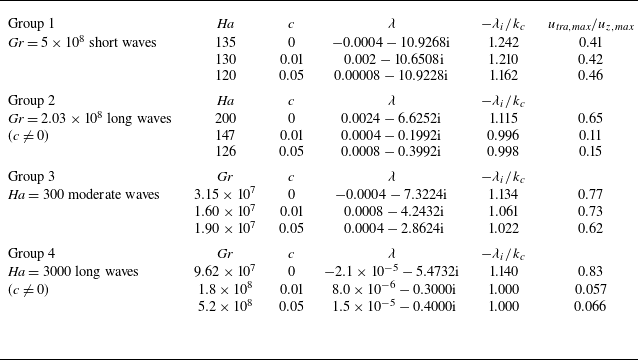
Table 2 shows the leading eigenvalue
 $\lambda =\lambda _r+\lambda _i\mathrm{i}$
and the phase speed
 $-\lambda _i\mathrm /k_c$
of the nearly neutrally stable modes at the selected parameters. It can be seen that, on the short-wave part of the moderate-
 ${\textit{Ha}}$
branch (group 1 in the table), the eigenvalues and the phase speeds of the three cases are close to each other, indicating that the wall conductivity does not affect the instability significantly. Similarly, no significant effects are observed on the moderate-wave part of the marginal stability boundary (see group 3 in the table). In contrast, as shown before, wall conductivity destabilises long waves on both the moderate-
 ${\textit{Ha}}$
and large-
 ${\textit{Ha}}$
branches of the marginal stability boundary (group 2 and 4), while long waves are linearly stable in the insulating-wall case. The frequency
 $\lambda _i$
is much smaller than its insulating-wall counterpart. Nevertheless, the phase speeds are still close given the much smaller wavenumber
 $k_c$
(see figure 4
b). The closeness of the phase speeds is determined by the flow structures of the perturbations and of the base flow, which are shown in the following.
Leading eigenvalue,
 $\lambda$
, and corresponding phase speeds,
 $-\lambda _i/k_c$
, of (nearly) neutrally stable modes at the four selected parameter groups on the marginal stability boundary. The last column is the ratio between the maximum transverse perturbation
 $u_{{tra,max}}=\mathrm{max}(\sqrt {u_x^2+u_y^2})$
and the maximum streamwise perturbation
 $u_{{z,max}}=\mathrm{max}(u_z)$
in the flow field.

Neutrally stable modes at
 ${\textit{Gr}}=5\times 10^8$
for wall conductance ratios
 $c=(a{-}c)\,0$
, (d–f) 0.01 and (g–i) 0.05. The corresponding
 ${\textit{Ha}}_c=135$
, 130 and 120, respectively. Contours of
 $u_z$
perturbation in the vertical
 $zOy$
plane, horizontal
 $zOx$
plane and the
 $xOy$
circular cross-section are shown. Arrows are the in-plane velocity vectors. Velocity is normalised by the maximum magnitude of
 $u_z$
perturbation in the field. Panels (a, c, d, f, g, i) share the same colourbar. Panels (b, e, h) share a colourbar with a much smaller range to visualise the much smaller velocity perturbations in the
 $xOz$
plane.

Figure 10 shows the critical mode of group 1, which is short waves in all the three cases. As the critical
 ${\textit{Ha}}_c$
values and the
 $k_c$
values are close to each other, the flow structures appear to be very similar, with perturbations concentrated close to the bottom wall while being very small in the rest of the circular cross-section. The velocity vectors in figure 10(a, c) indicate the perturbations form transverse convection rolls. However, because the rolls are located close to the bottom wall, they are bent down due to the constraint of the pipe wall. This flow structure is close to that reported for
 $c=0$
by Hu et al. (Reference Hu, Wu and Song2022) although the parameters there were not exactly on the marginal stability boundary. Nevertheless, although the perturbation in the lower half is the dominant one, it can be noticed in figure 10(c, f, i) that as
 $c$
increases, the perturbation in the upper part of the circular cross-section becomes slightly stronger. This indicates that the short-wave instability remains similar in all cases, and the small
 $c$
values considered here have no significant effects except for reducing the critical
 ${\textit{Ha}}_c$
and strengthening the upper-part perturbation slightly. The argument about the determining mechanism of the phase speed is similar as we gave in the previous section, i.e. the phase speed is largely determined by the basic-flow speed in the region where the perturbations are located.
Neutrally stable modes at
 ${\textit{Gr}}=2.03\times 10^8$
for wall conductance ratios
 $c=(a{-}c)\,0$
, (d–f) 0.01 and (g–i) 0.05. The corresponding
 ${\textit{Ha}}_c=200$
, 147 and 126, respectively. For each value of
 $c$
, from top to bottom,
 $u_z$
perturbation in the
 $zOy$
plane,
 $zOx$
plane and the
 $xOy$
circular cross-section. All velocity components are normalised by the maximum magnitude of
 $u_z$
perturbation in the field. Arrows are the in-plane velocity vectors. Each row shares the colourmap as indicated on the right end of the row, except for panel (b) which shares the colourmap with panels (a) and (c). Note that the vectors in panels (d) and (g) are stretched in the vertical direction according to the stretching of the vertical length scale. In fact, the streamwise velocity component is much larger than the vertical component.

Figure 11 shows the velocity field of group 2. The wavelength of the critical mode is more than one order of magnitude larger when the wall is conductive. In addition to the wavelength, significant differences in the flow structures are observed. Compared with the
 $c=0$
case where the perturbations form transverse convection rolls (see figure 11
a–c), in the conductive-wall cases,
 $u_z$
perturbations and in-plane perturbations are located much closer to the bottom and top pipe walls. Importantly, the in-plane velocities form vortex-like structures near the top wall (see figure 11
f, i), and this vortex is elongated in the streamwise direction indicated by the large wavelength. This vortex structure is a significant difference from the transverse convection rolls as in the insulating-wall case. The velocity vectors in the vertical
 $zOy$
plane still show convection roll structures, which are however elongated in the streamwise direction, but become much less aligned with the magnetic field (see figure 11
e, h). The relative amplitude of the transverse velocity component compared with the streamwise component, which is approximately 0.1 (see the last column of table 2), reveals that this long-wave structure is streamwise velocity dominant. In comparison, the transverse and streamwise velocities are comparable in amplitude, which is a characteristic of typical transverse convection rolls. One possible explanation of the appearance of the vortex structure is the following. As the transverse convection rolls move towards the pipe wall and get sufficiently close with increasing
 $c$
, the collective upward or downward motion associated with the convection rolls will be constrained by the curved wall of the pipe, which makes the vertical flow diverted and form in-plane vortex structure. As the perturbation covers nearly a half of the circular cross-section (see figure 11
f, i), it can be expected that the phase speed of the wave is close to the bulk speed of one, which is indeed the case (see table 2).
The appearance of long waves can be understood as follows. The transverse velocity is one order of magnitude smaller than the streamwise velocity as shown in table 2. Taking the streamwise velocity component to be
 $O(1)$
, the transverse velocity will be
 $O(0.1)$
. Therefore, for a fluid particle to take a cycle in a convection roll, which takes travelling a distance of
 $O(1)$
(the order of pipe diameter), it will be advected by a distance of
 $O(10)$
by the streamwise velocity in the same time period. This will form a convection roll that is elongated in the streamwise direction with a long streamwise wavelength of
 $O(10)$
.
Neutrally stable modes at
 ${\textit{Ha}}=300$
for wall conductance ratios
 $c=(a{-}c)\,0$
, (d–f) 0.01 and (g–i) 0.05. The corresponding
 ${\textit{Gr}}_c=3.15\times 10^7$
,
 $1.6\times 10^7$
and
 $1.9\times 10^7$
, respectively. For each value of
 $c$
, from top to bottom,
 $u_z$
perturbation in the
 $zOy$
plane,
 $zOx$
plane and the
 $xOy$
circular cross-section. Arrows are the in-plane velocity vectors. All velocity components are normalised by the maximum magnitude of
 $u_z$
perturbation in the field. Each row shares the colourmap as indicated on the right end of the row.

Figure 12 shows the velocity field of the critical mode of group 3. As
 $c$
increases, in addition to the increased wavelength, the flow structure becomes larger in the vertical direction and the location of the peak value of the
 $u_z$
perturbation moves towards the top and bottom wall (see figure 12
a, d, g). In addition to the left–right symmetry, the
 $u_z$
perturbation is nearly antisymmetric about the horizontal mid-plane, although the problem setting clearly has no symmetry about this plane due to the bottom heating. This is because
 ${\textit{Ha}}$
is relatively large and
 ${\textit{Gr}}$
relatively low, so that the magnetic effect is dominant on the flow and the flow is therefore nearly symmetric about this plane (see figure 5
c, h). The critical mode takes the form of transverse convection rolls that are nearly aligned with the magnetic field as shown in figure 12(b–i).
Neutrally stable modes at
 ${\textit{Ha}}=3000$
for wall conductance ratios
 $c=(a{-}c)\,0$
, (d–f) 0.01 and (g–i) 0.05. The corresponding
 ${\textit{Gr}}_c=9.62\times 10^7$
,
 $2\times 10^8$
and
 $5.2\times 10^8$
, respectively. For each value of
 $c$
, from top to bottom,
 $u_z$
perturbation in the
 $zOy$
plane,
 $zOx$
plane and the
 $xOy$
circular cross-section. Arrows are the in-plane velocity vectors. All velocity components are normalised by the maximum magnitude of
 $u_z$
perturbation in the field. Each row shares the colourmap as indicated on the right end of the row. Note that the vectors in panels (d) and (g) are stretched in the vertical direction according to the stretching of the vertical length scale. In fact, the streamwise velocity component is much larger than the vertical component.

Figure 13 shows the case of group 4. In the insulating-wall case (panels a–c), the perturbations also appear as transverse convection rolls aligned with the magnetic field. In the conductive-wall cases, similar to the long waves on the moderate-
 ${\textit{Ha}}$
branch, the flow also form vortex-like structures in the circular cross-section (see figure 13
f, i). Associated with the vortex structure, the wavelength is also large, being one order of magnitude larger compared with the insulating-wall case. The understanding of the formation of vortex structure and long wavelengths is presumably the same as we proposed for group 2.
To shortly sum up, even a small wall conductance ratio can affect the instability significantly. The most prominent effects include the destabilising effect at moderate
 ${\textit{Ha}}$
and stabilising effect at large
 ${\textit{Ha}}$
, and the excitation of long-wavelength unstable modes which exhibit streamwise vortex structures. In terms of phase speed, it appears that all critical modes investigated have phase speeds close to unity, especially for groups 2–4 in table 2. This is because the base flow is nearly uniformly unitary across the circular cross-section except for inside the thin boundary layers (see the
 $c\neq 0$
cases in figures 6 and 7) and, therefore, the perturbations are expected to be advected uniformly by the base flow and, hence, the phase speed of the perturbations would be close to unity. This suggests that the phase speed of the unstable modes is indeed approximately determined by the advection of the base flow.
5. Nonlinear saturated state
For the flow state after the perturbations have nonlinearly saturated (referred to as nonlinear saturated state hereafter), in the moderate-
 ${\textit{Ha}}$
regime of
 $O(10^2)$
, it was reported that close to the marginal stability boundary, the nonlinear saturated state is dominated by the unstable linear modes, reflected by the similarity between the flow structure of the nonlinear saturated state and that of the leading eigenmode (Zikanov et al. Reference Zikanov, Listratov and Sviridov2013; Hu et al. Reference Hu, Wu and Song2022). Similarly, in our simulations, the nonlinear saturated state close to the marginal stability boundary also appears to be dominated by the unstable linear mode in either the insulating wall or conductive wall case. Here, we will only show the flow at a few parameters in the interior of the linearly unstable region at the largest
 ${\textit{Gr}}$
considered. We select
 ${\textit{Gr}}=1\times 10^9$
, and for the insulating wall case, we select
 ${\textit{Ha}}=300,\,1000$
and
 $1\times 10^4$
, whereas we only consider
 ${\textit{Ha}}=300$
and 1000 for the conductive-wall cases because the flow is completely stabilised by the wall conductivity at
 ${\textit{Ha}}=10\,000$
. The aim is to see whether the flow can be turbulent or not and how the wall conductivity affects the nonlinear saturated flow with
 ${\textit{Gr}}=1\times 10^9$
. In the following studies, the flow is initiated with the base flow and small arbitrarily given perturbations of O
 $(10^{-4})$
on all Fourier modes. The flow will reach the nonlinear saturated state after sufficiently long time due to the underlying instabilities. We will only present the results for the nonlinear saturated state here.
5.1. Moderate magnetic field at
${\textit{Ha}}=300$

Velocity field of the nonlinear saturated flow at
 $(Ha,Gr)=(300, 1\times 10^9)$
. Contours of
 $u_z$
perturbation in the
 $xOy$
circular cross-section,
 $zOx$
plane and
 $zOy$
plane are shown from top to bottom. The perturbation here is defined as the deviation from the streamwise mean, i.e.
 $u_z-\langle u_z \rangle _z$
. Arrows are the in-plane velocity vectors. (a–c) For
 $c=0$
, (d–f) for
 $c=0.01$
and (g–i) for
 $c=0.05$
. Panels in each column share the same colour scale except for panel (b). The axial location of panels (a, d, g) corresponds to the location of the maximum
 $u_z$
perturbation.

Temperature field of the nonlinear saturated flow at
 $(Ha,Gr)=(300, 1\times 10^9)$
. Contours of
 $\theta$
perturbation in the
 $xOy$
circular cross-section,
 $zOx$
horizontal plane and
 $zOy$
vertical plane are shown from top to bottom. The perturbation here is defined as the deviation from the streamwise mean, i.e.
 $\theta -\langle \theta \rangle _z$
. Arrows are the in-plane velocity vectors. (a–c) For
 $c=0$
, (d–f) for
 $c=0.01$
and (g–i) for
 $c=0.05$
. Panels in each column share the same colour scale except for panel (b). The axial location of panels (a, d, g) corresponds to the location of the maximum
 $\theta$
perturbation.

Figures 14 and 15 show the cases at
 ${\textit{Ha}}=300$
and
 ${\textit{Gr}}=1\times 10^9$
. The pipe length is set to
 $9.8d$
, which is approximately 10 times of the wavelength of the leading unstable mode. For the discretisation, 384 Fourier modes (corresponding to 384 uniform grid points) are used in the axial direction and 192 Fourier modes are used in the azimuthal direction. In the radial direction, 144 grid points are used with the patched grid (see Appendix A). When the pipe wall is insulating, compared with the conductive-wall cases, the parameters are in fact relatively close to the marginal stability boundary (see figures 4
a or 9
a). Therefore, it can be expected that the nonlinearity will be relatively weak, reflected by the amplitude of the saturated velocity perturbation (O(0.01) in units of the mean flow speed
 $U_m$
, see the colourbar in figure 14
a). When the wall is conductive, due to the significant influence of the conductivity on the linear stability, as illustrated by the comparison between the linear stability boundaries as shown in figure 9, the marginal stability boundary moves to smaller
 ${\textit{Ha}}$
and longer waves are destabilised. Therefore, the point
 $(Ha, Gr)=(300, 1\times 10^9)$
becomes much farther from the marginal stability boundary compared with the insulating-wall case. Indeed, the flow structures are much more complicated with more wavelengths excited and even streamwise localisation, see figure 14(d–f) for the case of
 $c=0.01$
. The maximum magnitude of the velocity fluctuations is also several times larger than that of the insulating-wall case. The streamwise vortex structures in the conductive-wall cases, as shown in figure 14(d, g), may be the footprint of the long-wavelength unstable modes as shown in figure 12. Another point should be noted. Although the flow appears spatial and temporal complexities (see figure 16
a for temporal complexity), implying strong nonlinear effects, the distribution of velocity fluctuations however bear a left–right symmetry about the vertical plane through the pipe axis. Therefore, these nonlinear saturated states are still different from the classic pipe flow turbulence.
Figure 15 shows the temperature field of the saturated flow. In the
 $c=0$
case, the temperature perturbation is mainly concentrated near the bottom wall, similar to the velocity perturbation. The amplitude of the perturbation is also approximately
 $O(10^{-2})$
times of the base temperature (whose maximum is 0.12, see figure 8
a–c). Overall, the amplitude of the perturbation increases with increasing
 $c$
. It can reach
 $O(1)$
compared with the base temperature, and the maximum appears close to the left and right side walls (figure 15
d, g), which should be attributed to the stronger transverse circulations in the conductive cases. In a word, the temperature field confirms the destabilising effect of the wall conductivity in this moderate-
 ${\textit{Ha}}$
regime.
The non-dimensional average wall-shear stress
 $\tau _w=-\rho \nu ( {\partial \langle \mathrm{v}_z \rangle }/{\partial r})|_{r=0.5}/(\rho U_m^2)$
, where
 $\rho$
is the fluid density, and
 $\langle \boldsymbol{\cdot }\rangle$
denotes the average along streamwise and azimuthal directions, is shown in figure 16. In the insulating-wall case,
 $\tau _w$
appears constant, implying that the nonlinear saturated state shown in figure 14(a–c) may be a nonlinear travelling wave state. The flow visualisation in the
 $zOy$
plane at a few time instants is shown in figure 17. The flow appears to be a nonlinear travelling wave, because the flow structure is visually nearly frozen while being advected downstream the pipe (figure 17). However, slight variations of the flow structure, visualised by the contour lines, can be noticed by looking at the horizontal bar that is attached to the peak of the selected contour line in figure 17, whose distance to the top pipe wall varies slightly in time. Supplementary movie 1 (for velocity) and supplementary movie 2 (temperature) available at https://doi.org/10.1017/jfm.2026.11641 show more clearly the slight oscillation of the flow structure in the upper part of the pipe, while the dominant flow structures in the lower part travel downstream without noticeable changes.
Streamwise and azimuthally averaged wall shear stress
 $\tau _w$
of the nonlinear saturated flows. Panel (a) shows the time series of
 $\tau _w$
(solid) and the corresponding value of the basic laminar flow (dashed). The nonlinear and laminar values are nearly the same and cannot be distinguished for
 $c=0$
. Panel (b) shows the relative deviation of
 $\tau$
compared with the insulating case (
 $c=0$
).

Four snapshots for the saturated nonlinear state at
 ${\textit{Ha}}=300$
,
 ${\textit{Gr}}=1\times 10^9$
and
 $c=0$
. Contours of the streamwise velocity perturbation
 $u_z-\langle u_z\rangle _z$
, where
 $\langle \boldsymbol{\cdot }\rangle$
denotes the average along the axial direction, are plotted in the
 $zOy$
cross-section. The time increment between two consecutive snapshots from panels (a) to (d) is 0.4 time units (
 $d/U_m$
). The black horizontal bar on top of the contour line (close to the left-top corner in panel a) follows a structure and serves to visualise a slight variation of the flow structure over time, indicated by the slight changes in the distance of this bar to the top wall.

The
 $\tau _w$
of the nonlinear saturated flow and that of the basic laminar flow are visually indistinguishable in the insulating-wall case. The low amplitude of the streamwise velocity perturbation
 $u_z$
, which is
 $O(0.01)$
(the maximum is 0.016) as shown by the colourbar in figure 14(a), much smaller than the magnitude of the base flow, implies that the nonlinear effect is weak. In contrast, irregular spatial fluctuations and temporal complexities can be observed in the two conductive-wall cases (see supplementary movies 1 and 2). In addition, the amplitude of
 $u_z$
fluctuations reaches
 $O(0.1-1)$
in the conductive cases (the maximum is approximately 0.4, comparable to the magnitude of the base flow, see figure 14(d, g), indicating a much stronger nonlinearity in the velocity fluctuations. This observation confirms the destabilising effect of the wall conductivity on the nonlinear saturated state in this moderate-
 ${\textit{Ha}}$
regime, with the maximum velocity fluctuation being enlarged by more than one order of magnitude when
 $c$
in increased to 0.05.
The overall trend shows that
 $\tau _w$
increases with increasing
 $c$
. The corresponding
 $\tau _w$
of the basic laminar flow is also shown for comparison (see dashed lines in figure 16
a). Interestingly, the
 $\tau _w$
appears to be lower than the respective basic-flow value in the conductive wall cases. In other words, the driving pressure gradient needed in the nonlinear saturated state will be even lower than that in the laminar state. This reveals a complicated effect of the wall conductivity on the flow. Figure 16(b) shows the relative increase of the time-averaged
 $\tau _w$
compared with the insulating wall-case. It is seen that the wall conductance ratios considered in this work result in an increase of a few percent in the wall shear stress and, consequently, in the driving pressure gradient. However, it should be noted that the increase of
 $\tau _w$
is dictated by that of the base flow component (figure 16
a), i.e. the contribution of nonlinear perturbations only plays a minor role.
5.2. Strong magnetic field at
${\textit{Ha}}=1000$
and
$1\times 10^9$


Velocity field of the nonlinear saturated flow at
 $(Ha,Gr)=(1000, 1\times 10^9)$
. Contours of
 $u_z$
perturbation in the
 $xOy$
circular cross-section,
 $zOx$
plane and
 $zOy$
plane are shown from top to bottom. The perturbation here is defined as the deviation from the streamwise mean, i.e.
 $u_z-\langle u_z \rangle _z$
. Arrows are the in-plane velocity vectors. Panels in each column share the same colour scale. (a–c) For
 $c=0$
, (d–f) for
 $c=0.01$
and (g–i) for
 $c=0.05$
. The axial location of panels (a, d, g) corresponds to the location of the maximum
 $u_z$
perturbation.

Temperature field of the nonlinear saturated flow at
 $(Ha,Gr)=(1000, 1\times 10^9)$
. Contours of temperature perturbation in the
 $xOy$
circular cross-section,
 $zOx$
horizontal plane and
 $zOy$
vertical plane are shown from top to bottom. The perturbation here is defined as the deviation from the streamwise mean, i.e.
 $\theta -\langle \theta \rangle _z$
. Arrows are the in-plane velocity vectors. Panels in each column share the same colour scale. The axial positions of panels (a, d, g) are taken at the respective positions of the maximum
 $\theta$
perturbation, i.e. the same as those of panels (a, d, g) in figure 18. (a–c) For
 $c=0$
, (d–f) for
 $c=0.01$
and (g–i) for
 $c=0.05$
.

Figures 18 and 19 show the nonlinear saturated flow state at
 $(Ha, Gr)=(1000, 1\times 10^9)$
. The pipe length is set to
 $4\pi d$
, which is approximately ten times of the wavelength of the leading unstable linear mode at these parameters. For the discretisation, 384 Fourier modes are used in the axial direction and 192 Fourier modes are used in the azimuthal direction. In the radial direction, 192 grid points are used with the patched grid (see Appendix A). Based on the magnitude of the velocity perturbation, it can be seen that the insulating-wall case shows the strongest instability and the instability appears to weaken as
 $c$
increases, indicated by the decreasing amplitude of the perturbation (the maximum
 $u_z$
perturbation decreases from 0.46 at
 $c=0$
to 0.08 at
 $c=0.05$
). Regarding the flow structures, three cases exhibit similar flow structures, i.e. roll-cells aligned with the magnetic field. This can be clearly seen based on the in-plane velocity distribution in the
 $xOy$
and
 $zOy$
cross-sections. Specifically, velocities at the same altitude in the
 $xOy$
cross-section are collectively vertically up or vertically down (i.e. perpendicular to the magnetic field), corresponding to the up-going side or down-going side of a transverse convection roll. In addition, the flow in the
 $zOy$
cross-section shows nearly streamwise periodic structures that resemble the linear unstable modes. At
 $c=0$
, some amplitude modulation and multiple wavelengths can be observed, which are much weaker at
 $c=0.01$
and 0.05. Overall, the amplitude of the velocity perturbations decreases greatly as
 $c$
increases. All these observations confirm the stabilising effect of the wall conductivity on the velocity perturbation in the large-
 ${\textit{Ha}}$
regime.
Figure 19 shows the temperature perturbation of the saturated flow. Just as the velocity field, similarities can be seen in the temperature perturbation field in all three cases. The amplitude of the perturbation can also reach
 $O(0.1)$
compared with the base temperature (the maximum of the latter is approximately 0.28 according to figure 8
d–f). The most interesting observation is that the amplitude of the temperature perturbation appears to increase with increasing
 $c$
(see the maximum value given by the labels of the colourbar in figure 19
a, d, g). This observation indicates a destabilising effect of the wall conductivity on the temperature perturbation, in terms of amplitude, opposite to the stabilising effect on the velocity perturbation. This opposite effect cannot be expected from the linear stability analysis and must be due to nonlinear effects. This also indicates the complicated effect of the wall conductivity on the nonlinear saturated flow.
Streamwise and azimuthally averaged wall shear stress
 $\tau _w$
of the nonlinear saturated flows at
 $(Ha, Gr)=(1000,1\times 10^9)$
. Panel (a) shows the time series of
 $\tau _w$
(solid) and the corresponding value of the basic laminar flow (dashed). The nonlinear and laminar values are nearly the same and cannot be distinguished for
 $c=0.05$
. Panel (b) shows the relative deviation of
 $\tau$
compared with the insulating case (
 $c=0$
).

Figure 20 shows the time series of the wall-shear stress
 $\tau _w$
. Similar to the trend shown in figure 16,
 $\tau _w$
also increases with the wall conductance ratio
 $c$
. However, the deviation of
 $\tau _w$
of the nonlinear state from that of the basic laminar flow decreases with increasing
 $c$
, which is opposite to the trend for
 ${\textit{Ha}}=300$
. With
 $c=0$
, the nonlinear state shows irregular temporal fluctuations, while the
 $\tau _w$
with
 $c=0.01$
and 0.05 appears to be nearly constant over time, indicating that the flow states visualised in figure 18(d–i) are close to travelling wave states (see supplementary movie 3 for
 $u_z$
perturbation and supplementary movie 4 for temperature perturbation in the
 $zOy$
plane). This is consistent with the stabilising effect of the wall conductivity on the flow as revealed for the linear regime. The time averaged
 $\tau _w$
of the
 $c=0.01$
and 0.05 cases are 5.3 % and 7.6 % higher than that of the insulating-wall case, respectively (figure 20
b). As the value of the average
 $\tau _w$
of the nonlinear case is very close to that of the base flow, it can be concluded that the average wall friction is dictated by the base flow component.
Nonlinear saturated states at
 $(Ha,Gr)=(10000, 1\times 10^9)$
in the insulating-wall case. (a–c) Contours of
 $u_z$
perturbation in the
 $xOy$
circular cross section,
 $zOx$
plane and
 $zOy$
plane, respectively. The perturbation here is defined as the deviation from the streamwise mean, i.e.
 $u_z-\langle u_z \rangle _z$
. For comparison, panels (d–f) show the flow field of the leading linear eigenmode of the streamwise wavenumber
 $k=4.6$
(according to the dominant wavenumber as shown in panel b and c) at the same flow parameters. Arrows are the in-plane velocity vectors.

As
 ${\textit{Ha}}$
is increased to
 $1\times 10^4$
, the wall conductivity stabilises the flow; therefore, the flow will remain laminar or will laminarise in the conductive-wall cases. Here, we just show the results for the insulating wall case in figure 21. The same pipe length of
 $4\pi d$
as for the
 ${\textit{Ha}}=1000$
case is considered. For the discretisation, 192 Fourier modes are used in the axial direction and 192 Fourier modes are used in the azimuthal direction. In the radial direction, 192 grid points are used with the patched grid (see Appendix A). It can be seen that the nonlinear saturated flow structure appears to be convection rolls aligned with the transverse magnetic field, indicated by the collective upward or downward motion of the fluid at the same altitude (figure 21
a). The periodic streamwise arrangement of the rolls can be seen in figure 21(b, c). In addition, the total kinetic energy of the flow is a constant over time (not shown), indicating a nonlinear travelling-wave state. For comparison, the flow structure of the corresponding leading eigenmode of the same streamwise wavenumber as the dominant wavenumber of the saturated flow is shown in figure 21(d–f). Similarities between the linear mode and the nonlinear flow can be observed. Compared with the
 $c=0$
case at
 ${\textit{Ha}}=1000$
shown in figures 18(a–c) and 20(a), the flow is more stabilised at
 ${\textit{Ha}}=1\times 10^4$
as the parameters are closer to the marginal stability boundary (see figure 9
a).
6. Discussion and conclusion
In this paper, we studied the linear instability of liquid-metal mixed convection in a horizontal pipe with a strong transverse magnetic field. We selected
 ${\textit{Re}} =9046$
and
 $Pr=0.022$
as in former experimental and numerical studies (Genin et al. Reference Genin, Zhilin, Ivochkin, Razuvanov, Belyaev, Listratov and Sviridov2011; Zikanov et al. Reference Zikanov, Listratov and Sviridov2013; Hu et al. Reference Hu, Wu and Song2022), but extend the
 ${\textit{Ha}}$
greatly up to
 ${\textit{Ha}}=2\times 10^4$
and
 ${\textit{Gr}}$
up to
 $1\times 10^9$
. The parameters considered here nearly reach the estimated operation conditions for future nuclear fusion facilities:
 ${\textit{Re}} =O(10^4 - 10^5)$
,
 ${\textit{Gr}}=O(10^9-10^{12})$
and
 ${\textit{Ha}}=O(10^4-10^5)$
(Bühler Reference Bühler2007; Zikanov et al. Reference Zikanov, Belyaev, Listratov, Frick, Razuvanov and Sviridov2021; Chen et al. Reference Chen, Smolentsev and Ni2020, Reference Chen, Smolentsev and Ni2022). The aim of this study is to clarify whether the formerly discovered buoyancy-dominated instability persists under a strong magnetic field and study the effect of the wall conductivity. The main findings of our study are summarised as follows.
Our results revealed a marginal stability boundary in the large-
 ${\textit{Ha}}$
regime beyond which the linear instability will be fully suppressed. Therefore, the buoyancy dominated instability, which was concluded to appear under a strong magnetic field, cannot persist when
 ${\textit{Ha}}$
reaches
 $O(10^4)$
for
 ${\textit{Gr}}\lesssim 10^9$
. Nevertheless, the large-
 ${\textit{Ha}}$
branch, which seems to follow a power-law scaling of
 ${\textit{Gr}}\propto {\textit{Ha}}^{4/3}$
as
 ${\textit{Ha}}$
increases, suggests that this instability still can occur if
 ${\textit{Gr}}$
is sufficiently large. The relationship
 ${\textit{Gr}}\simeq 2100{\textit{Ha}}^{4/3}$
seems to fit the marginal stability boundary between
 ${\textit{Ha}}=4000$
and
 $2\times 10^4$
well, and can be used to estimate the onset of instability in this
 ${\textit{Ha}}$
regime. The linearly unstable modes in the large-
 ${\textit{Ha}}$
regime are still transverse convection rolls similar to those at moderate
 ${\textit{Ha}}$
reported before (Zikanov et al. Reference Zikanov, Listratov and Sviridov2013; Hu et al. Reference Hu, Wu and Song2022). Similar suppression effects of a sufficiently strong magnetic field of
 ${\textit{Ha}}\gtrsim 1000$
on magneto-convective fluctuations in vertical pipe configuration was reported (Belyaev et al. Reference Belyaev, Sardov, Melnikov and Frick2021), which is consistent with the scenario we found here. Akhmedagaev et al. (Reference Akhmedagaev, Zikanov and Listratov2022) reported instabilities up to
 ${\textit{Ha}}=1\times 10^4$
in horizontal duct flows at higher
 ${\textit{Gr}}$
than that considered here, which is consistent with the indication of our large-
 ${\textit{Ha}}$
branch. To suppress the linear instability at
 ${\textit{Gr}}=10^{10}$
in pipe flow, assuming the scaling
 ${\textit{Gr}}= 2100{\textit{Ha}}^{4/3}$
, requires
 ${\textit{Ha}}=1.02\times 10^5$
, which reaches the upper limit of the estimated operation condition for nuclear fusion facilities. Therefore, the analyses here suggest that this linear instability is likely relevant for real applications. However, caution should be taken about this estimation because the scaling remains to be confirmed for higher
 ${\textit{Ha}}$
.
Vo et al. (Reference Vo, Pothérat and Sheard2017) studied a similar problem in comparable
 ${\textit{Ha}}$
regimes in duct flow with the quasi-two-dimensional approximation. They showed a
 ${\textit{Gr}}{-} Ha$
scaling of the large-
 ${\textit{Ha}}$
branch, different from our results. This is likely attributed to the circular cross-section of pipe, which results in significantly curved isotherms even at
 ${\textit{Ha}}=O(10^4)$
(figure 8
d–f). Therefore, the isotherms are not parallel to the transverse magnetic field and the base temperature field cannot be treated as quasi-two-dimensional. This will create a variation of convection and diffusion contributions to the temperature distribution and consequently a varying buoyancy force along the convection rolls that are aligned with the magnetic field. However, how exactly this affects the instability behaviour remains to be clarified in the future. Vo et al. (Reference Vo, Pothérat and Sheard2017) also reported a sharp switch between short-wave and long-wave critical modes on the low-
 ${\textit{Ha}}$
branch even in the insulating-wall case, but that occurs at
 ${\textit{Ha}}\lesssim 30$
, much below the regime we considered here. As Hu et al. (Reference Hu, Wu and Song2022) pointed out, a similar switch also occurs in our configuration in the similar
 ${\textit{Ha}}$
regime because the instability mechanism will switch from buoyancy-driven to shear-driven as
 ${\textit{Ha}}$
is decreased. Therefore, the switch of the critical modes at low
 ${\textit{Ha}}$
observed by Vo et al. (Reference Vo, Pothérat and Sheard2017) is likely due to be the switch between the instability mechanisms also. Here, we only studied
 ${\textit{Re}} =9046$
, and whether the
 ${\textit{Gr}}\sim {\textit{Ha}}^{4/3}$
remains a general scaling when
 ${\textit{Re}}$
is varied and the underlying physical mechanism are interesting problems for future study. The results of Vo et al. (Reference Vo, Pothérat and Sheard2017) suggests such a possibility.
When the wall is electrically conductive, the base flow velocity is significantly affected, especially the velocity distribution in the vertical direction. The base flow becomes much more uniformly distributed in the core region of the circular cross-section. However, only modest effects of the wall conductivity on the base temperature field is observed. The calculation of the marginal stability boundary reveals the destabilising effect of the wall conductivity on the flow at moderate
 ${\textit{Ha}}$
and the stabilising effect in the large-
 ${\textit{Ha}}$
regime. In contrast to the insulating wall case where relatively short waves dominate, wall conductivity can also destabilise long waves in both the moderate-
 ${\textit{Ha}}$
regime and large-
 ${\textit{Ha}}$
regime, which exhibit much more streamwise elongated vortex structure that is distinct to typical structure of convection rolls in the insulating-wall case. Although velocity overshoots appear near the top and bottom wall sections when
 ${\textit{Ha}}$
is large, no inflectional instability as reported by Velizhanina & Knaepen (Reference Velizhanina and Knaepen2023) is observed in the parameter regime considered here. Presumably, much larger
 ${\textit{Re}}$
is needed for this inflectional instability to occur.
Nonlinear saturated flows were also simulated at
 ${\textit{Gr}}=1\times 10^9$
and the results also showed destabilising effects at moderate
 ${\textit{Ha}}=300$
and stabilising effects of the wall conductivity at large
 ${\textit{Ha}}=1\times 10^4$
on the nonlinear saturated flow, consistent with the finding of the linear stability analysis. In comparison, the saturated flow shows some spatial and temporal complexities when the wall is conductive in the moderate-
 ${\textit{Ha}}$
regime, but is less complex or even completely stabilised. Interestingly, in the intermediate regime at
 ${\textit{Ha}}=1000$
, results showed that the wall conductivity suppresses velocity perturbation but enlarges temperature perturbation, showing opposites effects on the velocity and temperature that cannot be predicted from the linear instability analysis. The underlying mechanism remains to be studied further. In both
 ${\textit{Ha}}$
regimes, the wall friction is increased by a few percent by the wall conductance ratios considered. The linear and nonlinear analyses both indicate that even a small wall conductivity can alter the instability and flow structures significantly. The stabilisation effect at
 ${\textit{Ha}}=10^4$
revealed here may suggest possible passive control methods on large-amplitude stress and temperature fluctuations by using a thin conductive wall, at the cost of a modest increase in the wall friction.
In this work, the quasi-static assumption is adopted given the small magnetic Reynolds number
 $R_m\sim O(10^{-3})$
. However, recently, Lalloz et al. (Reference Lalloz, Davoust, Debray and Pothérat2025) pointed out that the quasi-static approximation may not be always justified even in the case of low
 $R_m$
for a flow between two parallel walls driven by the forcing of an injected alternating electric current, depending on the forcing frequencies. Consequently, Alfvén waves may be present and important for the flow dynamics. This raises a question of whether the convection rolls resulting from the flow instability shown here can cause similar effects of the alternating forcing electric current and induce Alfvén waves in our problem. In addition, although the saturated flow structure at
 ${\textit{Ha}}=10^4$
resembles the leading linear mode, as shown in figure 21, it does not rule out the possibility that the flow state can also be reached via a subcritical mechanism. An example was shown in 2-D or quasi-2-D channel flows where a subcritical transition route via nonlinear Tollmien–Schlichting waves, which resemble their linear counterparts in structure, was identified (Camobreco, Pothérat & Sheard Reference Camobreco, Pothérat and Sheard2023; Huang et al. Reference Huang, Gao, Gao and Xi2024; Gao et al. Reference Gao, Wang, Chen, Xi and Huang2025). These possibilities are certainly interesting for future studies.
Supplementary movies
Supplementary movies are available at https://doi.org/10.1017/jfm.2026.11641.
Acknowledgements
The simulations were performed on Supercomputers provided by SuperComputing Network. Discussions with Jun Hu, Jinhan Xie and Ming Dong are acknowledged.
Funding
The authors acknowledge financial support from the National Natural Science Foundation of China (NSFC) (No. 12322209), NSFC Excellence Research Group Program for ‘Multiscale Problems in Nonlinear Mechanics’ (No. 12588201), NSFC grants No.12588301 and No.12272264. The work is also supported by The Fundamental Research Funds for the Central Universities, Peking University.
Declaration of interests
The authors declare no conflicting interests.
Author contributions
R. X. and G. C. have contributed equally to this work.
Appendix A. The patched grid for large
${\textit{Ha}}$

Here, we give more technical details about the patched grid used for
 ${\textit{Ha}}=1\times 10^4$
and
 $2\times 10^4$
. The three layers of our grid are sketched in figure 22 with their thickness specified. The thickness of the layers can adjust automatically according to the value of
 ${\textit{Ha}}$
. We use
 $N/2$
grid points in layer 1,
 $ {N}/{4}$
grid points in layer 2 and
 $ {N}/{4}$
grid points in layer 3, which in total gives a number of
 $N$
grid points in the radial direction.
Sketch of the patched grid. Layer 1 is used to resolve the core region. Layer 2, with a thickness of
 $7{\textit{Ha}}^{-1/2}$
, is used to resolve the Shercliff layer whose thickness is proportional to
 ${\textit{Ha}}^{-1/2}$
. Layer 3, with a thickness of
 $40{\textit{Ha}}^{-1}$
, is used to resolve the Hartmann layer whose thickness is proportional to
 ${\textit{Ha}}^{-1}$
. The thickness is normalised by the pipe radius
 $R$
.

In layer 1, we use a distribution
 \begin{align} \frac {r_{j}}{R}=\left(1-40{\textit{Ha}}^{-1}-7{\textit{Ha}}^{-1/2}\right)\dfrac {\sin ^{-1}\left (-\alpha \cos \left (\left(j+\frac {N}{2}\right)\pi /N\right )\right )}{\sin ^{-1}(\alpha )},\,\,\,\,j=1,2,\ldots ,\frac {N}{2}, \end{align}
where
 $R$
is the pipe radius and
 $\alpha$
is a stretching parameter. This distribution will approach uniform distribution when
 $\alpha$
approaches 1 and will approach the Chebyshev grid-point distribution when
 $\alpha \to 0$
. In this layer, we choose to use a rather uniform distribution by setting
 $\alpha =0.995$
.
In layer 2, we take a similar grid-point distribution
 \begin{align} \frac {r_{j}}{R}&=1-40{\textit{Ha}}^{-1}-7{\textit{Ha}}^{-1/2}+7{\textit{Ha}}^{-1/2}\dfrac {\sin ^{-1}\left (-\alpha \cos \left (\left(j-\frac {N}{4}\right)\pi /\frac {N}{2}\right )\right )}{\sin ^{-1}(\alpha )},\nonumber\\ j&=\frac {N}{2}+1,\ldots ,\frac {3N}{4}, \end{align}
in which the stretching parameter
 $\alpha =0.98$
. The points are nearly uniform close to layer 1 and are more clustered close to layer 3.
In layer 3, we take a half-set of a Chebyshev grid and map it into this layer, which is highly clustered close to the pipe wall and relatively sparse close to layer 2. The specific distribution reads
 \begin{equation} \frac {r_{N-j}}{R}=1-40{\textit{Ha}}^{-1}+40{\textit{Ha}}^{-1}\cos \left(j\pi /\frac {N}{2}\right),\,\,\,\,j=\frac {N}{4}-1,\frac {N}{4}-2,\ldots ,0. \end{equation}
The highly clustering characteristic near the wall helps to resolve the sharp gradient in the thin Hartmann layer at large
 ${\textit{Ha}}$
.
Next, we show some tests of the patched grid for calculating the base flow in the absence of the bottom heating, for which asymptotic/analytical solutions were reported. In the following, the total grid number is set to
 $N=256$
.
The asymptotic approximation of the core region (i.e. outside of the boundary layer) of the velocity profile on the vertical diameter, in the limit of large
 ${\textit{Ha}}$
, was given by Shercliff (Reference Shercliff1956), which reads
 \begin{equation} u_z(x=0,y) =u_z(x=0,y=0)\dfrac {(1+\textit{cHa})\sqrt {1-4y^2}}{1+\textit{cHa}\sqrt {1-4y^2}}, \end{equation}
and the velocity profile in the Hartmann boundary layer on the horizontal diameter is known to be (see e.g. Vantieghem et al. Reference Vantieghem, Albets-Chico and Knaepen2009)
 \begin{equation} u_z(x,y=0) =u_z(x=0,y=0)\left (1-\exp (\textit{Ha}(|2x|-1))\right ). \end{equation}
Note that there are slight differences with the referenced formula due to the different normalisations of length, i.e. it was normalised by pipe radius in the literature whereas by pipe diameter here. Figure 23 shows that, at
 ${\textit{Ha}}=1\times 10^4$
, our calculation overall agrees well with the theory for both velocity profiles, validating our numerical method. In the electrically insulating case
 $c=0$
, our calculation indicates that, the asymptotic approximation (A4) also captures the velocity in the near-wall region at large
 ${\textit{Ha}}$
. In contrast, in the electrically conductive case
 $c=0.01$
, the asymptotic approximation captures the core region well, but deviates from the actual velocity profile in the Roberts layer adjacent to the wall, in which a velocity overshooting appears (see figure 23
c), as shown by Vantieghem et al. (Reference Vantieghem, Albets-Chico and Knaepen2009).
Validation of the calculation of the streamwise velocity profiles for the non-heated flow at
 ${\textit{Ha}}=1\times 10^4$
. (a, b) Electrically insulating pipe wall. (c, d) Conductive wall with
 $c=0.01$
. (a, c) Profile on the upper half of the vertical diameter. The asymptotic approximation (A4) is shown as the red dashed curve. The inset in panel (c) shows a zoom-in view of the near-wall region. (b, d) Profile on the right half of the horizontal diameter. (A5) is plotted as the red dashed curve. Note that the horizontal axis in panels (b, d) shows the distance to the pipe wall,
 $0.5-x$
, in log-scale. The patched grid described in Appendix A is used for the calculation.

Figure 23(b, d) shows that the thickness of the Hartmann layer is approximately
 $5\times 10^{-4}D$
, where
 $D$
is the pipe diameter. Our Layer 3 is of a thickness of
 $40{\textit{Ha}}^{-1}R=2\times 10^{-3}D$
according to figure 22, covering the Hartmann layer well with 22 grid points inside the Hartmann layer by using
 $N=256$
. Layer 2 is of a thickness of
 $7{\textit{Ha}}^{-1/2}R=0.035D$
, which well covers the boundary layer near the top wall as shown in figure 23(c) with 64 grid points in
 $y\in (0.465, 0.498)$
by using
 $N=256$
. As can be seen, our setting of the patched grid can resolve the boundary layers well and give the correct velocity profiles at large
 ${\textit{Ha}}$
.
Appendix B. The Joule dissipation
In studies of the mixed convection of liquid metal flows subject to a magnetic field, in the context of blanket flow for nuclear reactors, the heating effect due to the Joule dissipation is usually ignored (see e.g. Bühler Reference Bühler2007; Knaepen & Moreau Reference Knaepen and Moreau2008; Zhang et al. Reference Zhang, Pan and Xu2013; Zikanov et al. Reference Zikanov, Listratov and Sviridov2013; Zhang & Zikanov Reference Zhang and Zikanov2014; Vo et al. Reference Vo, Pothérat and Sheard2017; Zhang & Zikanov Reference Zhang and Zikanov2018; Chen et al. Reference Chen, Smolentsev and Ni2020, Reference Chen, Smolentsev and Ni2022; Hu Reference Hu2020; Akhmedagaev et al. Reference Akhmedagaev, Zikanov and Listratov2022; Hu et al. Reference Hu, Wu and Song2022). Especially, this simplification was adopted even at extreme parameters with
 ${\textit{Ha}}\simeq 10^4$
(Vo et al. Reference Vo, Pothérat and Sheard2017; Zhang & Zikanov Reference Zhang and Zikanov2018; Chen et al. Reference Chen, Smolentsev and Ni2020, Reference Chen, Smolentsev and Ni2022; Akhmedagaev et al. Reference Akhmedagaev, Zikanov and Listratov2022; Zhang et al. Reference Zhang, Zhang, Li and Li2025). However, it was often not explicitly verified. Here, we briefly show two cases with and without considering the Joule dissipation.
Comparison between the magnitude of the different terms in the energy (B1). The amplitude of the Fourier coefficient of each term for the dominant azimuthal mode (with azimuthal wavenumber of
 $n=1$
) is used as a measure. The thin red curve represents the Joule dissipation term (the third on the right-hand side), the bold blue one represents the convection term
 $-\boldsymbol {u}\boldsymbol{\cdot }\boldsymbol{\nabla }\theta -u_z( {\mathrm{d}T_m}/{\mathrm{d}z})$
and the dashed black one is the diffusion term (the first term on the right-hand side).

Comparison between the solution of the base temperature and the temperature perturbation for simulations with and without the Joule dissipation. (a) Base temperature profile on the horizontal and vertical diameters. (b) Temperature perturbation profile on the horizontal and vertical diameters. The data are taken at the same time instant.

In the case with Joule dissipation, the equation for the temperature perturbation
 $\theta$
reads
 \begin{equation} \frac {\partial \theta }{\partial t} + \boldsymbol {u} \boldsymbol{\cdot }\boldsymbol{\nabla }\theta = \frac {1}{\textit{Pe}} {\nabla} ^2 \theta - u_z\frac {\mathrm{d}T_m}{\mathrm{d}z} + \frac {{\textit{Ha}}^2\textit{Re} }{\textit{Gr}}\frac {g\beta d}{c_p}\boldsymbol {j}^2, \end{equation}
where the last term on the right-hand side represents the contribution of Joule dissipation. The prefactor in the term needs to be determined by using the dimensional parameters
 $g$
,
 $\beta$
,
 $d$
and
 $c_p$
. This requires to choose a specific liquid metal and a specific pipe diameter. For this test, we choose liquid lead as the working fluid with
 $\beta =1.2\times 10^{-4}\,\mathrm{K}^{-1}$
,
 $g=9.81\,\mathrm{m\,s^{-2}}$
,
 $c_p=147\,\mathrm{J\,(kg\boldsymbol{\, }K)^{-1}}$
(Zikanov et al. Reference Zikanov, Belyaev, Listratov, Frick, Razuvanov and Sviridov2021) and
 $d=0.1 \,\mathrm{m}$
. Other parameters are taken as
 ${\textit{Ha}}=10^4$
,
 ${\textit{Gr}}=4.48\times 10^8$
and
 ${\textit{Re}} =9046$
. We consider the mode with the streamwise wavenumber
 $k=5.1$
, which is the critical mode at the given parameters.
For this calculation, we start from the same initial condition (with small perturbations) and run two simulations, one with the Joule dissipation term by solving (B1) and the other without the term as we did in the main text. Figure 24 shows the comparison between different mechanisms contributing to the change of the temperature, i.e. Joule dissipation, convection and diffusion based on the data from the simulation with the Joule dissipation term. The results show that, overall, the Joule dissipation is orders of magnitude smaller than other terms, especially in the core region. In the very thin boundary layers near the wall, it may reach comparable amplitude as the convection term, but is still much smaller than the diffusion term. Therefore, it can be expected that the results would not be affected significantly by dropping the Joule dissipation term. In fact, we obtained nearly indistinguishable evolution of the flow in the two simulations, see the temperature field at the same time instant shown in figure 25. For the exponential growth rate, we obtained
 $2.1768\times 10^{-4}$
and
 $2.1770\times 10^{-4}$
based on the data in exactly the same time period for the case with and without Joule dissipation, respectively, which are very close. The results shown here indicate that it is reasonable to drop the Joule dissipation, validating the assumption we adopted for the study in the main text.