1 Introduction
Reinforcement learning (RL) (Sutton & Barto Reference Sutton and Barto1998) has seen many successful applications, most recently with high visibility in Atari (Mnih et al., Reference Mnih, Kavukcuoglu, Silver, Rusu, Veness, Bellemare, Graves, Riedmiller, Fidjeland, Ostrovski, Petersen, Beattie, Sadik, Antonoglou, King, Kumaran, Wierstra, Legg and Hassabis2015) and Go (Silver et al., Reference Silver, Huang, Maddison, Guez, Sifre, van den Driessche, Schrittwieser, Antonoglou, Panneershelvam, Lanctot, Dieleman, Grewe, Nham, Kalchbrenner, Sutskever, Lillicrap, Leach, Kavukcuoglu, Graepel and Hassabis2016). Some of these applications, such as Go, exploit prior human experiences in the form of initial knowledge. Due to the high sample complexity of RL, many speed-up techniques have been proposed in the past, of which leveraging human demonstration has indeed proved to be highly successful. One relevant recent technique, called Human-Agent Transfer (HAT) (Taylor et al., Reference Taylor, Suay and Chernova2011), is framed as a transfer learning technique (Taylor & Stone Reference Taylor and Stone2009). It allows a human (a source agent) to demonstrate its policy, and a learner (the target agent) to bootstrap its learning based on this policy. A major distinction of this method from other work on learning from demonstration (LfD) is that an HAT learner seeks to eventually outperform the demonstrator, rather than just to reproduce the demonstrator’s policy (as in imitation, or apprenticeship, learning).
Given the success of demonstration-based RL in single-agent settings, and HAT in particular, it is natural to ask to what extent can this technique be used in a multi-agent RL setting? We are particularly interested in framing collaborative multi-agent teams within the HAT framework. One obvious dilemma with multi-agent LfD is regarding the size of the team trainable by human demonstration. On the one hand, it may be difficult for a single human to demonstrate multi-agent control when the number of autonomous agents in the team is large. On the other hand, requiring multiple human demonstrators—each controlling one or a small number of agents—delegates the question of agent coordination to that of coordination among the human demonstrators themselves. However, for teams of small sizes, it may be quite easy for a human to demonstrate effective coordination and help the team bootstrap RL. Hence we focus on small teams in this article. In particular, our experiments are in two-agent problem domains.
This article investigates the following two questions. First, does the advantage of HAT extend to multi-agent systems? In particular, is a team of autonomous agents able to exploit human demonstration to bootstrap RL as much as a single agent? We show that, compared to single-agent HAT where the initial performance (and often the asymptotic performance as well) of a HAT-agent is better than an unbiased agent, the difference is dramatically more pronounced in multi-agent HAT. In some of our experiments, the unbiased RL agents were completely unable to learn the tasks, whereas with multi-agent HAT, they were able to learn with a reasonable sample complexity and even outperform the demonstrator. We ground this investigation on two recent HAT methods: confidence-based HAT (CHAT) and dynamic reuse of prior (DRoP).
Second, given that the demonstrator’s global view of the task state can differ from the individual agents’ (local) view of the state, what impact does this difference have on the performance of multi-agent HAT? In particular, agents following human demonstrations with respect to their individual observations may select actions different from what the human demonstrator would have picked with a global view of all agents’ observations. We propose a novel confidence-based technique— coordination confidence (CC)—that predicates the confidence of its action recommendations on this difference, allowing the team to improve its learning rate in our experimental domains. The confidence values for states seen in the demonstration are computed in a pre-training, off-line phase, which are then deployed during multi-agent learning in an efficient way even for novel states. CC is found to boost learning rates in two ways: (1) when the confidence is high, it can lead to novel action recommendations compared to baselines, which can aid coordination; and (2) when the confidence is low indicating that the difference in global and local perspectives is critical, it recommends learning instead of exploiting the demonstration, which helps the agents avoid miscoordination.
2 Related work
There has been very little work on training a team of autonomous agents from demonstration in the past, where the environment is partially observable; that is, agents have different (partial and local) views of the global state. Chernova and Veloso (Reference Chernova and Veloso2007) proposed the confident execution learning framework where a Gaussian mixture model is trained for each action class in the demonstration data, exploiting its built-in confidence in a new classification to either select the model prediction (when confidence is high) or request new demonstration (when confidence is low). Chernova and Veloso argued that this approach was highly suited for multi-agent learning especially in domains requiring agent coordination, since expert guidance can allow it to learn much faster compared to explorative multi-agent RL where discovering coordinated joint actions can be extremely challenging. Furthermore, the approach shows a reduced demand on the expert over time, making it practically viable. While we use one of their application domains (Furniture Movers) for experiments, our setting differs in that we do not access a demonstrator after the initial demonstration; that is, no additional demonstration is required.
Reinforcement learning as a rehearsal (RLaR) (Kraemer & Banerjee, Reference Kraemer and Banerjee2016) is a related approach, where rather than a complete demonstration, an external entity (which could be a human) informs the learning agents about the parts of their state spaces that are hidden from their view, enabling them to perform RL as a rehearsal, but the agents must learn policies that do not rely on the hidden parts of their states. In da Silva et al. (Reference da Silva, Glatt and Costa2017), similar online feedback is exchanged among the agents themselves, but in this work we seek to limit any advice to be an off-line prior, thus limiting the need for communication during learning.
One recent related work (Le et al., Reference Le, Yue, Carr and Lucey2017) seeks to exploit sports tracking data as demonstration for coordinated multi-agent imitation learning. This scenario also has multiple demonstrators, but they play a more passive role, and their coordination—often implicit in such data, and modeled as a latent variable— is the target of inference. Another recent work (Song et al., Reference Song, Ren, Sadigh and Ermon2018) extends generative adversarial imitation learning (GAIL) to multi-agent settings, with demonstrations generated by multiple experts—one for each learning agent. GAIL (meant for a single learning agent) poses the problem of imitation learning as a competitive game between a discriminator and a generator, where the discriminator is trained to discriminate between the learning agent’s trajectories and those of the expert, while the generator controls the learning agent’s policy that attempts to generate trajectories indistinguishable from the expert’s. Song et al. (Reference Song, Ren, Sadigh and Ermon2018)’s adaptation of GAIL for general Markov games is called MAGAIL (multi-agent GAIL), and it encompasses cooperative, competitive, and mixed settings among multiple learning agents. Similar to our work, MAGAIL does not assume access to the expert after the initial demonstration. However, both of these approaches belong to the category of imitation learning, and as previously distinguished from the goal of imitation learning, we seek to exploit the demonstration to enable our agent team to eventually outperform the demonstrator team.
3 Background
This section discusses relevant background, including RL, LfD, and HAT, and a recent advance to the latter.
3.1 Reinforcement learning
RL problems are modeled as Markov Decision Processes or MDPs (Sutton & Barto, Reference Sutton and Barto1998). An MDP is given by the tuple  $\langle S,A,R,P\rangle$, where S is the set of visible environmental states that an agent can occupy at any given time; A is the set of actions from which it can select one at a given state;
 $R:S\times A \mapsto \mathbb{R}$ is the reward function—that is, R(s,a) specifies the reward from the environment that the agent gets for executing action
 $a\in A$ in state
 $s\in S$; and
 $P:S\times A\times S\mapsto [0,1]$ is the state transition probability function specifying the probability of the next state in the Markov chain following the agent’s selection of an action in a state. The agent’s goal is to learn a policy
 $\pi:S\mapsto A$ that maximizes the sum of current and future rewards from any state s, given by,
 \begin{equation}V^{\pi}(s^{0})=E_{P}[R(s^0,\pi(s^0))+\gamma R(s^1,\pi(s^1))+\gamma^2R(s^2,\pi(s^2))+\cdots],\end{equation}
where  $s^0,s^1,s^2,\ldots$ are successive samplings from the distribution P following the Markov chain with policy
 $\pi$.
RL algorithms, bereft of any prior knowledge of P or R, often evaluate an action-quality value function Q given by
 \begin{equation}Q(s,a)=R(s,a)+\max_{\pi}\gamma \sum_{s'}P(s,a,s')V^{\pi}(s').\end{equation}
This quality value stands for the sum of rewards obtained when the agent starts from state s, executes action a, and follows the optimal policy thereafter. Model-free RL methods directly learn Q(s,a) by online stochastic approximation, for example, Q-learning (Sutton & Barto, Reference Sutton and Barto1998):
 \[Q(s,a)\gets Q(s,a)+\alpha[r+\gamma\max_{a'}Q(s',a')-Q(s,a)],\]
where r and s′ are sampled from R and P, respectively. The final policy is calculated as
 \begin{equation}\pi(s)=\arg\max_a Q(s,a).\end{equation}
3.2 Learning from demonstration
While often effective, RL can suffer from slow learning rates. One way of learning faster is to re-frame the problem to that of mimicking a demonstrator. In this case, the agent typically solves a supervised learning problem so that it can perform similarly to a demonstrator (Argall et al, Reference Argall, Chernova, Veloso and Browning2009). While the majority of such LfD methods assume there is only a single-agent learning, there are some methods (Chernova & Veloso, Reference Chernova and Veloso2007) that allow the demonstrator to provide demonstrations to individual agents in a multi-agent setting. Additionally, LfD methods typically assume that the demonstrator is near-optimal—even if there is an environmental reward signal, LfD methods typically do not use it to improve the policy.
To speed up RL, there are many methods for incorporating biases that can help an agent learn faster. One approach is to combine the sample-efficient learning of LfD with the reward-seeking behavior of RL, as discussed in the next section.
3.3 Human-Agent Transfer
HAT (Taylor et al., Reference Taylor, Suay and Chernova2011) reimagines demonstration-based learning from the perspective of transfer learning (Taylor & Stone, Reference Taylor and Stone2009), where knowledge gained from a prior task (often referred to as source task) is used as inductive bias to bootstrap RL in a related but different task (often referred to as target task). In lieu of a related source task, HAT views the demonstration itself as initial bias (coming from a source agent) that informs the RL’s action choices, but gradually weans RL off this bias as the RL’s own value function improves over time. In particular, the idea of HAT, in a single-agent context, engages the following steps:
1. Induce a supervised classifier with the demonstration, to approximate the source agent’s policy
 $\pi_{Source}:S\mapsto A$.
2. Bootstrap RL with the trained classifier, that is, instead of acting randomly as an RL agent would initially, use the classifier for action selection, but only with a probability,
$\Phi$, that decreases over time. Thus an $\epsilon$-greedy RL agent would select action as follows: select an action randomly with probability $\epsilon$, select the classifier’s predicted action with probability $\Phi$, or select action according to Equation (3) with probability $1-\Phi-\epsilon$.


Even though the demonstration may cover a small part of the state space, with a sufficiently rich representation of states the classifier’s capability of generalization can be effectively leveraged to predict what the demonstrator’s actions might have been in unseen states. Thus, the classifier can serve as a powerful initial bias for RL. Different types of classifiers have been used in the past, for example, decision trees, neural networks, and Gaussian processes (Wang & Taylor, Reference Wang and Taylor2017). Typically, an initial comparative analysis of different classifiers on the available demonstration data can inform the choice of the most appropriate classifier.
The above framework was originally introduced as probabilistic policy reuse (Fernandez et al., Reference Fernandez, Garcia and Veloso2010), where  $\Phi$ is called the policy reuse parameter. More recently, Wang and Taylor (Reference Wang and Taylor2017) leveraged the confidence in the classifier predictions to decide whether to rely on its prediction, or on RL’s value function, in a refined framework called CHAT. However, this framework still uses the policy reuse parameter
 $\Phi$, which typically starts close to 1 but decays exponentially to enable the agent to rely more on its (increasingly better) learned action value function over time. The choice of the decay factor may pose a difficult tuning problem; too rapid decay may make RL rely prematurely on its learned Q-values, resulting sometimes in a temporary drop in performance and an associated ‘valley’ in the learning curve. On the other hand, if the decay in
 $\Phi$ is too slow, then the performance of the learner, even when mature, can be skewed in the learning curve by the classifier’s own performance. To address this dilemma, Wang and Taylor (Reference Wang and Taylor2019) introduced a new variant of CHAT that does not require explicit decay of the reuse parameter, described in the next section.
3.4 Dynamic reuse of prior
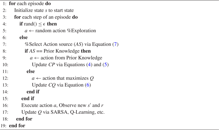
The DRoP algorithm (Wang & Taylor, Reference Wang and Taylor2019) builds upon HAT by adding an online confidence measure to the transferred data. In particular, Step (1) in HAT, as described in the previous section, is modified so that a confidence measure of the classifier is learned (i.e., the classifier can output both a label and a confidence for a given input). Step (2) is modified as described next, and then summarized in Algorithm 1.Footnote 1
DRoP

A confidence-based temporal difference (TD) model is used to analyze the performance level of every action source with respect to every state. The confidence in the classifier of prior knowledge for a given state, CP(s), is initialized to be the confidence of the classifier, and is updated by the following equation over time:
 \begin{equation} CP(s)\leftarrow (1-\alpha) \times CP(s) + \alpha \times [G(r)+\gamma \times CP(s')],\end{equation}
where  $\gamma$ is the discount factor, r is the reward, and
 $\alpha$ is the update parameter. The reward is normalizedFootnote 2 based on the confidence in the different actions:
 \begin{equation} G(r)= \frac{r}{r\_max}\times \max \left\{ \frac{1}{\sum_{i} exp(\lambda_{i}^T\cdot x)}\begin{bmatrix}exp(\lambda_{1}^T\cdot x))\\exp(\lambda_{2}^T\cdot x))\\...\\exp(\lambda_{i}^T\cdot x))\end{bmatrix}\right\},\end{equation}
where  $\frac{r}{r\_max}$ is a normalized reward (
 $r\_max$ denotes the maximum absolute reward value) and G(r) re-scales the reward using the confidence distribution. Equation (5) shows one way of computing the confidence distribution: via a softmax layer in a neural network with weights
 $\lambda_i$, and x being the input to that layer for state s. In our experiments, we use random forest classifier with its confidence distribution from Weka, instead of a neural network.
The confidence in the Q-value of a given state, CQ(s), is initialized to be zero. It is updated over time via the following equation:
 \begin{equation} CQ(s)\leftarrow (1-\alpha) \times CQ(s) + \alpha \times [r+\gamma \times CQ(s')].\end{equation}
We use a probabilistic action selection mechanismFootnote 3:
 \begin{equation} AS ={\begin{cases} Q & P=\frac{\tanh \left({rCQ} \right) +1}{\tanh \left( rCP \right) +\tanh \left({rCQ} \right) +2} \\ Prior & P=\frac{\tanh \left({rCP} \right) +1}{\tanh \left( rCP \right) +\tanh \left({rCQ} \right) +2} \end{cases}}\end{equation}
where  $rCP(s)=CP(s)/R$,
 $rCQ(s)=CQ(s)/R$, and
 $R=\max_s\{|CP(s)|, |CQ(s)|\}$. Thus, a high confidence in prior knowledge makes following the prior knowledge more likely, and a low confidence in the prior knowledge makes it less likely. Equation (7) can be easily extended to settings with multiple priors,
 $CP_i$, by setting the likelihood of selecting
 $CP_i$ as an action source to
 $P=\{\tanh(rCP_i)+1\}/\left[\sum_k \{\tanh(rCP_k)+1\}+\{\tanh(rCQ)+1\}\right]$.
4 Human multi-agent transfer
Human multi-agent demonstrations are collected as joint-state joint-action vectors  $\left<\vec{s},\vec{a}\right>$, where the state
 $s_i$ of the ith agent in the team is a feature vector over its local sensor data. Agents must learn to map their own states to their own actions (
 $\pi_i:S_i\mapsto A_i$); therefore, the demonstration can be separated out agent-wise, and the ith agent can be given its own portion of state-action demonstration,
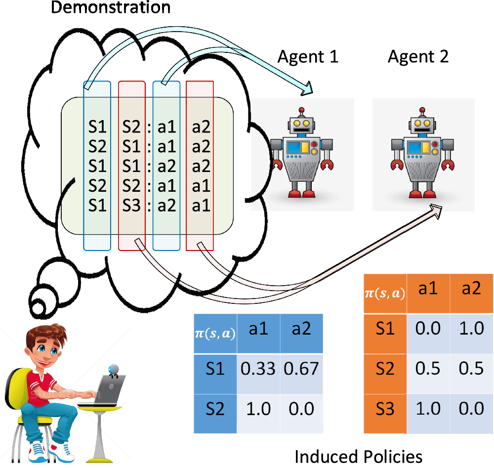
 $\left<s_i,a_i\right>$, to use as prior as shown in Figure 1. This is a straightforward extension of HAT to a multi-agent setting. However, as we argue in the following, this first-cut approach may not work well in some domains.
The human-multi-agent transfer framework

4.1 Difference in perspectives
An important difference between the human demonstrator and the agents is the difference in perspectives. In single-agent LfD, the human and the agent will perceive the task environment through different sets of sensors, raising the question whether, or to what extent, the policy of one is usable by the other. In a multi-agent setting, this question is of magnified import. The demonstrator usually sees the global state (i.e., the states of all agents in the team) and demonstrates actions for all agents. However, each agent is only capable of observing its own local state, and can only execute its own actions. This scenario is depicted in Figure 1 for a two-agent team. While the demonstrator records joint actions against joint states, agents induce classifiers that map their individual states to individual actions. In the example of Figure 1, the induced policies will only be perfectly coordinated when the agents observe joint state  $\left< S2,S1 \right>$. For joint states
 $\left<S1, S1\right>$ and
 $\left< S2, S2\right>$, they will be miscoordinated 33% and 50% of the time, respectively, but in joint state
 $\left<S1, S2\right>$ they will be miscoordinated over 83% of the time. It seems in the last case the agents are better off randomly exploring instead of following the demonstrator’s recommendation. Notice that an agent cannot infer such states (where the risk of miscoordination is high) from its own classifier’s confidence alone. For example, in state
 $\left<S2, S2\right>$, even though Agent 1’s classifier is fully confident about recommending action a1, Agent 1 will still be miscoordinated 50% of the time, because it does not know Agent 2’s state (and hence its confidence at that step). This insight is a key contribution of this article.
4.2 Coordination-based prior
The key to solving the above problem is to note that the information needed to predict when an agent might be more prone to miscoordination when following the human demonstration is already present in the joint demonstration  $\left<\vec{s},\vec{a}\right>$. Therefore, we propose to make the entire joint demonstration available to each agent, so that each agent can perform an independent off-line analysis that can be used later to predict where the agent is more (or less) likely to be miscoordinated with its teammates. This information can be seen as an additional prior for each learning agent, apart from the individual policy induced from the human demonstration. We discuss the methodology in detail next, introducing a solution to our novel multi-agent problem.
5 Coordination confidence
This article focuses on collaborative team tasks of identical payoff games, where every agent in the team receives the same reward. Joint actions that are coordinated lead to higher values of the agents’ payoffs, while miscoordinated joint actions lead to poor payoffs. The coordinated joint actions form the Nash equilibrium (Fudenberg & Levine, Reference Fudenberg and Levine1998) of the game, the highest valued ones being Pareto dominant. While a Nash equilibrium assumes a probabilistically independent choice of agent actions, when the agent choices are somehow correlated, the resulting equilibrium—called a correlated equilibrium—can provide higher payoffs to the agents in identical payoff games (Fudenberg & Levine, Reference Fudenberg and Levine1998). However, the latter requires a correlation device—a signal that is commonly observed by the agents. One view of our idea of coordination-based prior is that apart from the commonly observed reward, the joint demonstration serves as an additional correlation device, observed as an off-line prior, but used online during RL. We speculate that this additional correlation device may allow the agents to learn a higher valued correlated equilibrium than those that do not have access to this device. We now discuss how the agents distill this correlation device into a confidence measure to bias independent RL.
5.1 Off-line analysis
Given the agent-specific demonstration,  $\left <s_i,a_i\right >$, the ith agent trains a classifier via supervised learning,
 $\mathcal{ C}_i:S_i\mapsto\Delta A_i$, that returns a confidence distribution over its actions. But since it also receives the entire demonstration, it can also train such classifiers for other agents
 $j\neq i$,
 $\mathcal{ C}_j:S_j\mapsto \Delta A_j$, as well as a single classifier that maps a joint state to a confidence distribution over joint actions,
 $\mathcal{ C}:S\mapsto\Delta A$. Then, given a state
 $s_i$, the agent computes a confidence measure that indicates that if it follows its classifier then the agent will be coordinated with the other agents, as
 \begin{equation}\theta(s_i) = 1-\frac{\sum_{s_j\in\vec{s},j\neq i}\|\otimes_{j}\mathcal{ C}_j(s_j)-\mathcal{ C}(\vec{s})\|_2N_{j,i}}{M_i\sqrt2},\end{equation}
where  $\otimes$ is the Cartesian product,
 $N_{j,i}$ is the number of times in the full demonstration where the ith agent’s state was
 $s_i$ while the others’ state matched
 $s_j$,
 $M_i$ is the number of times in the full demonstration where the ith agent’s state was
 $s_i$, and
 $\sqrt2$ is the required normalization factor for norm-2 distance between probability distributions. Because
 $\sum_{s_j}N_{j,i} = M_i$ and the maximum norm-2 distance between two probability distributions is
 $\sqrt{2}$,
 $\theta(s_i)$ in Equation (8) is bounded in [0,1]. At one extreme, if
 $\theta(s_i)=1$, then agent i can expect that if it uses
 $\mathcal{ C}_i$ and other agents use their classifiers, then their joint action will be perfectly coordinated. In other words, the agent’s local view
 $s_i$ of the joint state
 $\vec{s}$ is completely sufficient for it to select the proper action. At the other extreme,
 $\theta(s_i)=0$, which means that if it uses
 $\mathcal{ C}_i$ and other agents use their classifiers, then their joint action will be perfectly miscoordinated. That is, the agent’s local view
 $s_i$ of the joint state
 $\vec{s}$ is insufficient; someone with a global view of
 $\vec{s}$ would be able to select a coordinated joint action where i’s portion
 $a_i$ was deterministically different.
Although the computation of  $\theta(\cdot)$ is lower bounded by
 $\Omega(|\otimes_i A_i|)$, which is exponential in the number of agents, it is performed off-line and hence the cost is amortized.
5.2 Computation of coordination confidence: an illustration
Here we illustrate the computation of CC by Agent 1 in the example of Figure 1, for the two cases:  $s_i=S1$ and
 $s_i=S2$. We use i and j to be synonymous with Agents 1 and 2, respectively.
5.2.1 When Agent 1 observes S1
Suppose Agent 2 also observes  $s_j=S1$. Then according to Figure 1,
 $\mathcal{C}_i(S1)=\left<0.33,0.67\right>$ and
 $\mathcal{C}_j(S1)=\left<0,1\right>$. Therefore, the Cartesian product of the agents’ action distributions,
 $\mathcal{ C}_i(S1)\otimes\mathcal{C}_j(S1)$, for the joint state
 $\left<S1, S1\right>$ is computed as

However, the joint classifier induced from the demonstration is  $\mathcal{C}(\vec{s}=\left<S1, S1\right>)$ is

since only joint action  $\left <a_2,a_2\right >$ is ever taken at that joint state. Hence, the difference of these distributions is
 \begin{equation*}\|\mathcal{C}_i(S1)\otimes\mathcal{ C}_j(S1)-\mathcal{ C}(\left <S1, S1\right >)\|_2 = \sqrt{(0-0)^2 + (0.33-0)^2 + (0-0)^2 + (0.67-1)^2 }=0.4714.\end{equation*}
Similarly, considering the other possible states for Agent 2 when Agent 1 observes S1, we get the confidence distributions over the joint actions as

Therefore, Agent 1’s CC value in state  $S_1$ will be
 \begin{equation*} \theta(s_i=S1) = 1-\frac{(0.4714 + 0.9718 + 0.4714) \times (N_{j,i}=1,\forall s_j)}{(M_i=3)\times\sqrt2} = 0.5487.\end{equation*}
The small value of  $\theta(S1)$ above captures the essential intuition described in Section 4.1 when Agent 1 observes S1 but is unaware of Agent 2’s observation.
5.2.2 When Agent 1 observes $S_2$

The confidence distributions over the joint actions in this case are given by

Consequently, Agent 1’s CC value in state S2 will be
 \begin{equation*} \theta(s_i=S2) = 1-\frac{(0 + \sqrt{1/2}) \times 1}{2\sqrt2} = 0.75.\end{equation*}
This shows that Agent 1 can be more confident of not miscoordinating with Agent 2 when following its individual classifier  $\mathcal{C}_i$ in state S2, than when its state is S1.
5.3 Online use of coordination confidence
Let the states of agent i visited during the demonstration form the subset  $S_i^D\subset S_i$. During explorative RL, the agent will potentially visit many other states not seen by the demonstrator. Rather than training an inductive regressor to predict
 $\theta$ for such states, we apply transductive or instance-based prediction. For a state
 $s_i\in S_i\setminus S_i^D$, we optimistically predict
 \begin{equation} \begin{array}{l} \bar{\theta}(s_i)=\max\{\theta(s_i')|s_i'\in\Sigma_{s_i}\},\\ \Sigma_{s_i}=\{s_i'|d(s_i,s_i')\le d(s_i,s_i'')\le\epsilon,\forall s_i',s_i''\in S_i^D\}, \end{array}\end{equation}
where d is a feature distance measure. In words, among all of agent i’s states in the demonstration that are closest (by distance measure d) to  $s_i$ but not farther than
 $\epsilon$,
 $\bar{\theta}$ optimistically selects the highest
 $\theta$ confidence using Equation (8). Depending on the choice of
 $\epsilon$,
 $\Sigma_{s_i}$ could be empty for some
 $s_i$, in which case
 $\bar{\theta}$ is set to 0. This online computation is
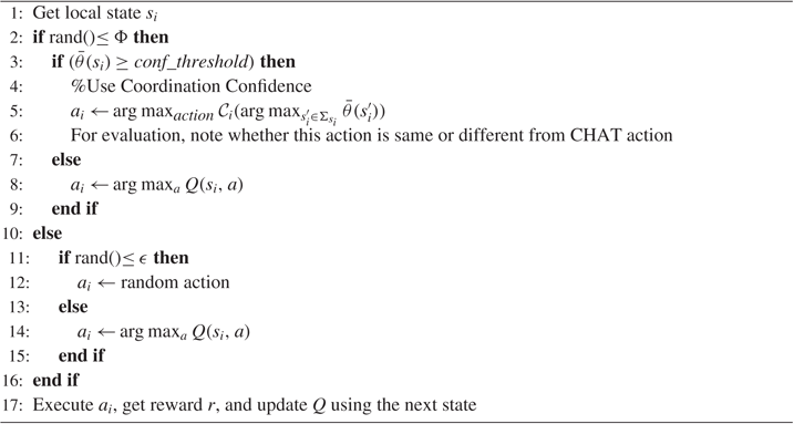
 $O(|S_i^D|^2)$, hence a constant for a fixed amount of demonstration. Algorithm 2 shows the CC-Agent algorithm, which opts for CC when it is high, but otherwise falls back on Q.
6 Experimental evaluation
We use three domains for experimental evaluation: Furniture Movers (Chernova & Veloso, Reference Chernova and Veloso2007), Guided Navigation, and Block Dudes. We describe these domains in the following subsections, and present the experimental results alongside, with parametric settings that were selected via preliminary parameter search experiments trying roughly 20 combinations of the parameters in each domain. In all experiments, we used random forest as the classifier because of its improved accuracy in all domains compared to other classifiers reported in previous literature. The result of this preliminary analysis, performed in Weka 3.8.1, is shown in Table 1.
Training set size, and classifier accuracies by F-Measure averaged over 10-fold cross validation, performed on human demonstration (training set) in the three experimental domains. All experiments used the default parameters in Weka. The lengths of the human demonstration episodes are summarized in the ‘Human’ column of Table 2.

In the experimental results that follow, we study the following learning algorithms:
CC: This is an implementation of Algorithm 2, instantiated for each agent. When reporting the action choice frequencies of CC, we use the labels ‘CC = CHAT’ and ‘CC != CHAT’ to distinguish the counts according to line 6 of Algorithm 2, yielding whether or not the CC agent’s actions are the same as what a CHAT learner’s classifier would have produced for the same state.
CHAT: This is an implementation of the CHAT algorithm from Wang and Taylor (Reference Wang and Taylor2017), instantiated for each agent. This learner’s action counts are not of interest, since there is only one prior (the demonstration) and the rate of prior usage decays predictably with  $\Phi$. Hence its action counts are not separately reported.
DRoP: This is an implementation of Algorithm 1, instantiated for each agent. When selecting an action source via Equation (7) (line 7 of Algorithm 1), a DRoP agent uses two separate ‘Priors’ in Equation (7): CC and CHAT. The CHAT prior takes the action that its classifier recommends, and the CC prior takes the action from line 5 of Algorithm 2. The modified version of Equation (7) for multiple priors is given at the end of Section 3.4.
When reporting the performance of various learning agents in these domains in the following sections, we collect the performances of the agents from multiple ( $\ge\!\!30$) independent trials in each domain, and show the 95% confidence intervals of the performance measure in the form of band plots. Thus any two curves whose bands are well separated exhibit a statistically significant (at the 95% level) difference in performance.
CC_Agent_i(conf_threshold)

6.1 Furniture Movers
6.1.1 Domain description
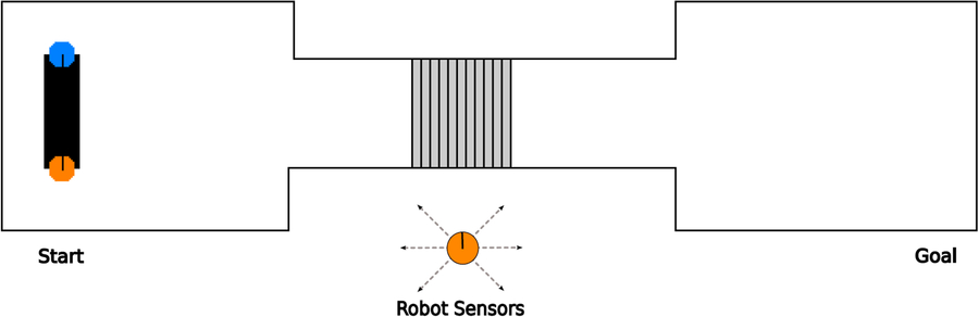
The Furniture Movers domain is shown in Figure 2, adopted from Chernova and Veloso (Reference Chernova and Veloso2007). We first give the original description of this domain from Chernova and Veloso (Reference Chernova and Veloso2007) and then specify customizations used in this article.
Furniture Movers domain from Chernova and Veloso (Reference Chernova and Veloso2007)

Two agents are jointly tasked with moving a long and heavy piece of furniture from the room on the left to the one on the right, through a narrow corridor which also has a staircase. Each agent has a set of six range sensors as shown, each giving it a noisy reading of the nearest obstacle in that direction. An agent can also sense the stairway, but only when next to (or on) it. An agent can move in one of the four cardinal directions, or execute a ‘stair’ action. Agents can successfully navigate the stairway only when both execute the ‘stair’ action (although both may not be able to see the stairway), otherwise they stay stuck. Furthermore, joint actions that make the agents lose their grip on the furniture (e.g., moving in opposite directions) also do not change their locations. Apart from the five actions, an agent can also execute a communicate action to inform the other if it sees the stairs, to enable coordination for joint ‘stair’ action. Thus the state feature vector of each agent has, in addition to the six range sensor measurements, two binary stair features, one for its own location and one for its teammates. The teammate’s stair feature can only be updated via the communicate action from the other. As in Chernova and Veloso (Reference Chernova and Veloso2007), the movements of the agents are discretized, and the task can be completed optimally in 39 steps, indicating that the joint start and goal locations were fixed.
We made the following changes to this domain:
As movements are discretized, we allow each agent to move in any of the eight directions, rather than four. This expands the action space of each agent, making the joint learning problem even more challenging for independent Q-learners, especially without any prior.
We select the joint start locations randomly within the left room, and the joint goal location is set to be anywhere in the right room. That is, agents can start anywhere in the left room, both holding the furniture at its opposite ends, and as soon as both are located anywhere in the right room (again both holding the furniture), we say that the episode has ended successfully. These settings were the same for the human demonstrator, as for the experiments.
We introduced 10% action noise for joint actions; that is, agents’ joint actions are changed randomly 10% of the time after they have selected their actions, but before the actions are executed in the environment. However, the changed actions are not allowed to include communicate. The purpose of this noise is to create variations in the demonstrated trajectories, since the demonstrator could otherwise follow a fixed trajectory after the agents have successfully entered the narrow corridor.
We set the reward function to be –1 for all actions, except the joint action that ends the episode successfully, which has a reward of
$+100$ for each agent.

6.1.2 Experimental results in Furniture Movers
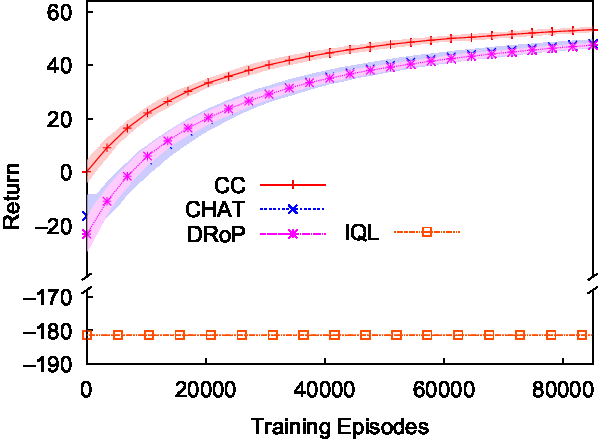
Because of the first three changes, the optimal episode length is no longer 39, and only fixed in expectation. The task is extremely challenging to independent Q-learners (IQLs) with no prior, to the extent that they are completely unable to learn, with all learning episodes being capped at 200 steps, as shown in Figure 3. This figure shows the cumulative average of the discounted episode returns obtained by the learners, with each plot point being averaged over 32 independent trials. Each agent used  $\epsilon=0.05$,
 $\gamma=0.999$, and
 $\alpha=0.005$; CHAT and CC used a confidence threshold of
 $0.7$, and a
 $\Phi$ decay rate of
 $0.999977$. With an experiment horizon of
 $1.5\times10^5$ episodes, this decay rate reduces
 $\Phi$ to
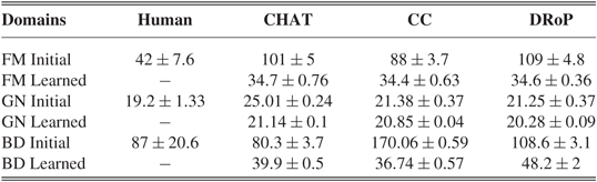
 $\approx 0.03$. Figure 3 shows that in contrast with IQL, all three versions of HAT are able to learn this task, CC outpacing CHAT and DRoP at a statistically significant rate. Furthermore, Table 2 shows the initial and learned episode lengths (average of first 20 000 and last 20 000 episode lengths, respectively) of these three algorithms in this task, together with the demonstrator’s performance for comparison. Here we see that CC has a higher jump-start (difference in initial performance, from no-prior IQL) than CHAT and DRoP, but all three algorithms ultimately learn to perform similarly. Note that they learn to outperform the human demonstrator.
Learning curves in Furniture Movers. Episode lengths were capped at 200 steps, which IQL always reached.

Summary of episode lengths (lower is better) in Furniture Movers (FM), Guided Navigation (GN), and Block Dudes (BD). Total learning episodes were  $1.5\times 10^5$,
 $10^5$, and
 $3.0\times 10^6$, respectively.

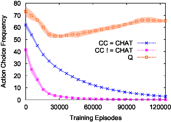
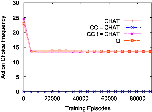
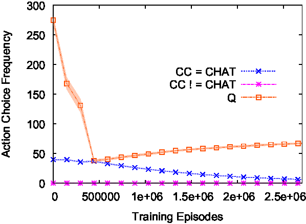
In order to further investigate the performance improvement of CC over CHAT, we scrutinized the action choices of Algorithm 2, particularly how often it selected actions by CC (line number 5), or Q (line numbers 8, 14). Furthermore, when Algorithm 2 chose an action recommended by CC, we also compared them to those that CHAT would recommend, that is, whether the recommendations would have differed from CHAT (line number 6). Figure 4 shows the result of this experiment, with a moving window average over a window size of 20 000 episodes, averaged over 32 trials. Clearly, the CC-Agent leverages CC quite often, especially early. Also notice the high frequency of CC  $\neq$ CHAT, which stands for the action choices that are solely attributable to CC and are distinct from CHAT’s classifier. Although this rate tapers off due to
 $\Phi$ decay (as does the rate for CC = CHAT, while the rate of Q-value utilization replaces them), the distinct action choices prompted by CC explain the superior jump-start and learning rate of CC-Agent. Figure 4 shows the actual action counts; thus, the sum of the counts at any episode is also close to the episode length (sans the
 $\epsilon$ exploration).
Action choice frequency (sum over two agents) of the two sources in Algorithm 2: CC or Q, in Furniture Movers. The CC count is further broken into whether the action is same as CHAT or different.

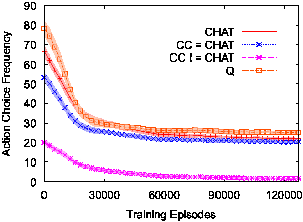
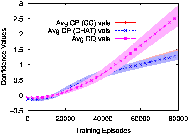
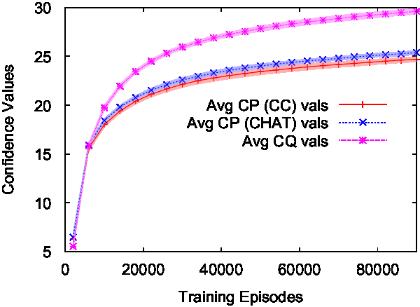
Figure 5 shows the action choice frequency of DRoP due to various sources of confidence: CC, CHAT, or Q; with a moving window average over window size of 20 000 episodes, averaged over 32 trials. Since DRoP does not decay the rate of prior usage, we see that all three sources continue to be used (with Q being slightly dominant for the most part), although overall rates fall because learning shortens the episodes, reducing the number of actions chosen. Also notice that CC (i.e.,  $\text{CC} = \text{CHAT} + \text{CC} \neq \text{CHAT}$) is not a dominant source, unlike in Figure 4 in the early part, which means that DRoP is unable to leverage the unique information conveyed by CC, which would explain why it performed similarly to CHAT, and underperformed in Figure 3. Finally, Figure 6 shows the actual values of confidence from different sources for DRoP, verifying that Q is indeed mostly dominant as a source.
Action choice frequency (sum over two agents) of various sources for DRoP, in Furniture Movers. Action selection driven by three different sources: CHAT, Q, or CC. The last count is further divided into if the action is same as CHAT or not.

Average confidence values of three sources for DRoP, per agent, in Furniture Movers

6.2 Guided Navigation
6.2.1 Domain description
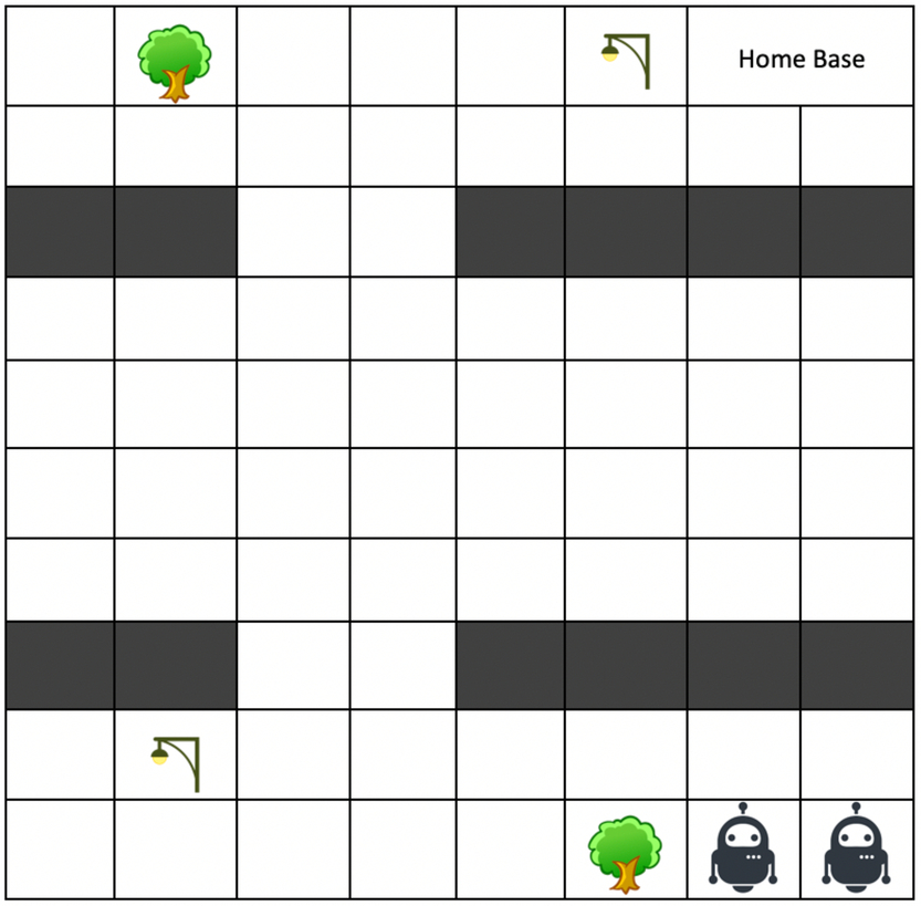
We introduce a new domain, Guided Navigation, shown in Figure 7. It is a simple grid navigation task on a  $10\times8$ gridmap. Two agents are jointly tasked with crossing a street from the footpath below to reach the home base on the top, through a narrow crossing. The agents always move as a pair, and they have different (complementary) sets of sensors. The leading Agent (Agent 1) has a set of 10 sensors which sense the obstacles in the 10 cells surrounding the 2 agents, whereas Agent 2 can only sense its current position (x and y coordinates of itself and, by inference, of Agent 1 as well). Thus Agent 1 can sense any obstacle only when the obstacle is within the immediate surrounding of the agents; Agent 2 lacks this near vision but has access to the global position of the pair. The agents can move in any of the four cardinal directions but only when both the agents execute the same action simultaneously, otherwise they stay stuck. The domain has four static obstacles along the footpath (two street light poles and two trees) and two dividers on both sides of the street with a narrow path to cross the street. The task can be completed optimally in 17 steps (without actuation noise), with both the agents reaching the home base simultaneously. The starting, goal, and obstacle locations are fixed in the domain. We added 10% noise in joint actions, but there is no sensor noise.
Guided Navigation domain

6.2.2 Experimental results in Guided Navigation
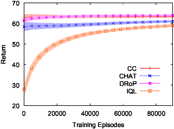
Figure 8 shows the cumulative average of the discounted episode returns obtained by the learners, with each plot point being averaged over 30 independent trials. Each agent used  $\epsilon=0.05$,
 $\gamma=0.99$, and
 $\alpha=0.01$; CHAT and CC used a confidence threshold of
 $0.7$, and
 $\Phi$ decay rate of
 $0.99997$. CC used a distance threshold of
 $2.5$. All episodes are capped at 200 steps, and the experiment horizon is
 $10^5$ episodes. Figure 8 shows that all three versions of HAT as well as IQL are able to learn this task, CC and DRoP outperforming CHAT at a statistically significant rate. All three HAT variants have a higher jump-start compared to IQL.
Learning curves in Guided Navigation domain

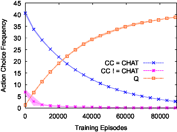
Similar to Furniture Movers, we scrutinized the action choices of Algorithm 2, particularly how often it selected actions by CC (line number 5) or Q (line numbers 8 and 14). Figure 9 shows the result of this experiment, with a moving window averaged over a window size of 20 000 episodes, averaged over 30 trials. Initially a vast majority of the actions are prompted by source CC. Even though CC  $\neq$ CHAT actions are far fewer relative to CC = CHAT actions, they probably dominate in key states where CHAT would miscoordinate, which may be why CC outperforms CHAT in Figure 8. As the experiment proceeds, the frequency of actions taken from CC-Agent are increasingly prompted by source Q values. Note that the sum of the counts at any episode is also close to double the episode length (as the action counts are summed over the two agents in each episode).
Action choice frequency (sum over two agents) of the two sources in Algorithm 2: Q or CC in Guided Navigation. The CC count is further broken into whether the action is same as CHAT or different

Figure 10 shows the action choice frequencies of DRoP. Again these counts are based on moving window averaged over window size of 20 000 episodes, averaged over 30 trials. We notice that all three sources continue to be used, although overall rates fall because learning shortens the length of episodes, reducing the number of actions chosen. Interestingly, unlike in Furniture Movers (i.e., Figure 5), CC  $\neq$ CHAT is used rather often as a source, which means DRoP is able to exploit the unique insights offered by CC, which might explain its comparable performance in Figure 8.
Action choice frequency (sum over two agents) of various sources for DRoP: CHAT, Q or CC in Guided Navigation. The CC count is further broken into whether the action is same as CHAT or different

Figure 11 shows the confidence values of different sources for DRoP, verifying that Q is indeed mostly dominant as a source.
Action confidence values of three sources for DRoP, per agent, in Guided Navigation

6.3 Block Dudes
6.3.1 Domain description
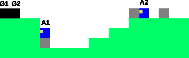
We introduce a new challenging domain for cooperative multi-agent planning and learning, called Block Dudes. It is based on a Texas Instruments (TI) calculator puzzle concept as implemented in BURLAP (MacGlashan, Reference MacGlashan2014), but with two agents instead of one. An implementation of this domain with text-based rendering, as an OpenAI Gym environment, is publicly available at https://github.com/RAILUSM/gym-envs/tree/master/two_agents. The initial state is depicted in Figure 12. The agents, marked A1 and A2 (blue, with an eye showing its current heading), are located in some landscape, along with three blocks (gray). The goal of agent i is to reach the cell marked Gi (black). The initial configuration is such that the agents are incapable of reaching the goal without using the blocks. Furthermore, the world is two dimensional, so the agents cannot pass each other, or co-occupy any cell. Thus, the quickest way for the agents to reach their goals is to cooperate and pass blocks from right to left to stack at the bottom of the cliff, creating a stairway to climb up to their goals.
Block Dudes domain

Each agent is only capable of local sensing, to know its own location, heading, and whether it is currently carrying a block. Further, an agent can sense the features of the other agent when within a horizontal distance of 4, but not otherwise. However, we found that merely local sensing the blocks made independent RL difficult; therefore, following the implementation in BURLAP, we made all blocks visible to both agents at all times. Note that this allows an agent to infer the location of the other agent if the latter is carrying a block, even when they are farther apart than 4 units. An agent’s action space contains five actions: east, west, up, pickup, and putdown. The directional actions, east and west, either changes the heading of the agent, or progresses it one step in the direction of its heading, as long as this is allowed by the terrain. The action up allows the agent to climb up a block (irrespective of whether or not it is carrying a block) that is in front of it and at the same level. The actions pickup allows the agent to pick up a block that is in front of it and at the same level; putdown allows it to drop a block that it is carrying as long as the height of the terrain in front of the agent is no larger than the height of the agent. As with our modification of Furniture Movers, we added 10% joint action noise, but there is no sensor noise.
The variance of the demonstrator in Block Dudes was high (see Table 2) because certain action choices (either by mistake, or by action noise) can lead to dramatically different trajectories. For instance, if A2 drops a block at the edge of a step, then A1 will neither be able to pick it up, nor be able to climb over, because in either case it needs to be at the same level as the block. This necessitates a costly detour where A1 goes back to grab the leftmost block and use it to regain access to the inaccessible block. While the human demonstrator was repeatedly frustrated by such unexpected calls for replanning, the learners were able to minimize them (evident from their lower variance), for example, by dropping blocks early. Some demonstrations ended in failure because the blocks had been configured in ways that made it impossible to achieve the joint goal. Such demonstrations were discarded. In the end, 11 successful demonstrations were collected. The human demonstrator found this task challenging because of unforeseen variations, but also frustrating because noise often preempted future plans.
6.3.2 Experimental results in Block Dudes
The reward function in this domain is similar to Furniture Movers:  $+100$ to each agent only when both agents are in their respective goal cells, −1 for all other situations. Because this domain appeared challenging, we reduced the learning rate to
 $\alpha=0.001$, and slowed the
 $\Phi$ decay rate to
 $0.9999992$, but kept the other parameters (
 $\epsilon$ and
 $\gamma$) unchanged from Furniture Movers. When reporting performances with windowed averages, we raised the window size from 20 000 in the previous domains to 50 000 in this domain, and ran our experiments for
 $3\times 10^6$ episodes with 30 trials. Notice the
 $\Phi$ decay is slower here due to the increased experiment horizon;
 $\Phi$ decays to
 $\approx 0.09$. Despite the slow decay of
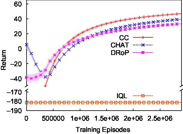
 $\Phi$, the ‘valley’ mentioned in Section 3.3 still appeared in the learning curve of CHAT in Figure 13, exhibiting the difficulty of tuning this parameter with the learning rate. Note that this domain, similar to Furniture Movers, is challenging enough that IQL never learns.
Learning curves in Block Dudes domain. Episode lengths were capped at 200, which IQL always maxed out.

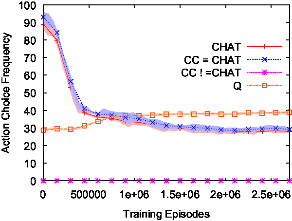
It is noteworthy in Figure 13 that CC has a poor initial performance (it starts within the break in the vertical axis), but eventually outperforms all other algorithms. The action choice frequency plot of CC-Agent (Figure 14) shows why CC-Agent has a poor initial performance. It shows a relatively high usage of Q-values initially, which indicates that CC confidence is often low; therefore, the agents prefer to learn rather than exploit the demonstration. This may in fact allow the learners to avoid miscoordination early on (miscoordination may be another reason why the performance of CHAT drops at first, displaying the ‘valley’ characteristic), eventually leading to superior performance. DRoP does not exhibit the ‘valley’ characteristic of CHAT that depends on a decaying prior reuse rate. However, its asymptotic performance is lower than CC or CHAT.
Action choice frequency (sum over two agents) of various sources in Algorithm 2: CHAT, Q, or CC, in Block Dudes. The last count is further broken into whether the action is same as CHAT or different.

Finally, Figure 15 shows the action choices of DRoP due to the three sources, CC, CHAT, and Q. In contrast with Figure 5, the HAT sources dominate initially, with the learned Q function eventually exploited more often. But the initial dominance of HAT sources explains the improved learning rate of DRoP.
Action choice frequency (sum over two agents) of various sources for DRoP in Block Dudes. Action selection driven by three different sources: CHAT, Q, or CC. The last count is further broken into whether the action is same as CHAT or different.

7 Conclusion
We have verified via experiments in three domains that HAT, when extended to multi-agent RL, is indeed advantageous for agents to bootstrap RL, but to a greater extent in multi-agent systems than in single-agent RL as studied in the past. While it imparts a jump-start and improves the learning rate in single-agent systems, multi-agent systems may be completely unable to learn without demonstration in some challenging tasks.
We have proposed a method to measure the degree of confidence that agent teams can have regarding coordination in demonstrated data, and leverage this confidence for action selection. We have found that this information can be advantageous in two ways: (1) when high confidence leads to coordinated action choices, and (2) when low confidence avoids usage of demonstration preventing miscoordination. Both of these effects can have a positive impact on the learning rate as well as the asymptotic performance.
We have also verified the difficulty of parameter tuning for the decay of prior reuse rate in HAT derivatives, and that a recently proposed technique to avoid this tuning in single-agent systems, called DRoP, can indeed avoid the ‘valley’ in learning curves in multi-agent learning. This can result in faster learning for the team. However, we found that DRoP may not achieve similar jump-start as CHAT, which may call for a more informed way to initialize the confidence values of various sources of priors in DRoP.
Our method is applied in two stages: off-line computation of CC and online usage of CC. While the first stage can be exponential in team size, the second stage is applied individually by the agents and is polynomial in the size of the demonstration. Since the first stage is off-line and amortized, the overall method is scalable for discrete state and action spaces. However, it is not immediately clear what effects continuous state/action spaces might have on scalability, especially the first stage, since the second stage (Equation (9)) can still be applied with no change except for a suitable distance function. Since such problems would inherently require some form of function approximation, it is conceivable that Equation (8) could be computed for only the observed states, and a value function approximation model (e.g., a neural network) could be trained to produce CC as an additional output. The complexity of off-line computation would be no worse in this case. This, however, assumes discrete actions. Problems with continuous actions might need to compute Equation (8) in a fundamentally different way, and this constitutes an important direction for future research.
Acknowledgments
We thank the anonymous reviewers for constructive comments and suggestions. This work was supported in part by National Science Foundation grant IIS-1526813.