1 Introduction
While the rising/settling dynamics of rigid objects in a homogeneous fluid has raised considerable interest, the influence of a density stratification of the fluid on the motion of a body is a much more complex problem which has gained interest in recent years. Such a fluid environment is, however, encountered in many environmental and industrial situations, where transport and mixing processes are related to the settling of biomass or pollutants to the bottom of the ocean or in the atmosphere. In particular, in marine biology it is desirable to gain a better understanding of the dynamics of microorganisms in a stratified environment (MacIntyre, Alldredge & Gotschalk Reference MacIntyre, Alldredge and Gotschalk1995), of their role in mixing (Wagner, Young & Lauga Reference Wagner, Young and Lauga2014; Wang & Ardekani Reference Wang and Ardekani2015; Houghton et al. Reference Houghton, Koseff, Monismith and Dabiri2018) and of their potential influence on the general circulation of the oceans (Wunsch & Ferrari Reference Wunsch and Ferrari2004). The influence of density gradients on the dispersal of pollutants is likewise an essential question for waste-water disposal in the ocean (Koh & Brooks Reference Koh and Brooks1975), as it is for the quality of the atmosphere (Fernando et al. Reference Fernando, Lee, Anderson, Princevac, Pardyjak and Grossman-Clarke2001). Also, atmospheric events, such as dust storms and volcanic eruptions (Carazzo & Jellinek Reference Carazzo and Jellinek2012), have a strong impact on air traffic and require further investigation and modelling.
Among the variety of freely moving bodies investigated for a homogeneous fluid, the disk of finite thickness is particularly interesting. Anisotropy of the body plays an important role in the motion of the body, especially when the velocity of the body departs from its principal axis, corresponding to axial symmetry (Ern et al. Reference Ern, Risso, Fabre and Magnaudet2012).
For a disk of finite thickness  $h$, diameter
 $d$ and density
 $\unicode[STIX]{x1D70C}_{d}$ evolving in a homogeneous fluid of density
 $\unicode[STIX]{x1D70C}$ and kinematic viscosity
 $\unicode[STIX]{x1D708}$, the motion of the body depends on three parameters. First we define the Archimedes number
 $$\begin{eqnarray}Ar=\sqrt{(\unicode[STIX]{x1D70C}_{d}/\unicode[STIX]{x1D70C}-1)gh}d/\unicode[STIX]{x1D708},\end{eqnarray}$$
which is analogous to the Reynolds number ( $Ud/\unicode[STIX]{x1D708}$) based on the gravitational velocity
 $U_{g}=\sqrt{(\unicode[STIX]{x1D70C}_{d}/\unicode[STIX]{x1D70C}-1)gh}$ (
 $g$ being the gravitational acceleration) instead of the observed velocity
 $U$. The two other parameters are the density ratio
 ${\mathcal{R}}$, and the geometrical aspect ratio
 $\unicode[STIX]{x1D712}$ given by
 $$\begin{eqnarray}{\mathcal{R}}=\unicode[STIX]{x1D70C}_{d}/\unicode[STIX]{x1D70C}\quad \text{and}\quad \unicode[STIX]{x1D712}=d/h.\end{eqnarray}$$
The buoyancy-driven motion of a disk in a homogeneous fluid has been thoroughly investigated experimentally (Willmarth, Hawk & Harvey Reference Willmarth, Hawk and Harvey1964; Field et al. Reference Field, Klaus, Moore and Nori1997; Fernandes et al. Reference Fernandes, Risso, Ern and Magnaudet2007), numerically (Auguste, Fabre & Magnaudet Reference Auguste, Fabre and Magnaudet2010; Chrust, Bouchet & Dušek Reference Chrust, Bouchet and Dušek2013) and theoretically (Fabre, Auguste & Magnaudet Reference Fabre, Auguste and Magnaudet2008; Tchoufag, Fabre & Magnaudet Reference Tchoufag, Fabre and Magnaudet2014). These works mainly focus on the different non-rectilinear and non-vertical paths, along with their characteristics which are observed above a critical Archimedes number  $Ar_{c}({\mathcal{R}},\unicode[STIX]{x1D712})$ that depends on the density ratio and the aspect ratio. Among these, periodic motions are observed and associated with an unsteady wake and the periodic release of vortices. Below
 $Ar_{c}$, the body follows a rectilinear vertical path associated with a stationary flow in the frame moving with the body. This path corresponds to a broadside-on type of motion, where the principal axis of the disk is aligned with the velocity. Disks dropped with different initial inclination angles tend to orient themselves with their face normal to the direction of motion, indicating that a single stable position exists for the disk in this regime. This behaviour is observed for Reynolds numbers that are greater than approximately
 $0.1$ (this critical value depends on the body shape), whereas in the Stokes regime, the body retains its original orientation as it falls (McNown & Malaika Reference McNown and Malaika1950).
From a general point of view, in the case of a continuously stratified fluid characterized by its Brunt–Väisälä frequency
 $$\begin{eqnarray}N=\sqrt{-\frac{g}{\unicode[STIX]{x1D70C}_{0}}\frac{\text{d}\unicode[STIX]{x1D70C}}{\text{d}z}},\end{eqnarray}$$
where  $\unicode[STIX]{x1D70C}_{0}$ is a reference density for the background density
 $\unicode[STIX]{x1D70C}(z)$, the dynamics of moving objects is governed by two additional parameters, the Froude number
 $Fr=U/Nd$ and the Schmidt (or Prandtl) number
 $Sc=\unicode[STIX]{x1D708}/\unicode[STIX]{x1D705}$ (or
 $Pr=\unicode[STIX]{x1D708}/\unicode[STIX]{x1D705}$) describing the competition between diffusive effects in the fluid, we denote
 $\unicode[STIX]{x1D705}$ as the diffusion coefficient of the stratifying agent. Experimental (Yick, Stocker & Peacock Reference Yick, Stocker and Peacock2007; Biró et al. Reference Biró, Gábor Szabó, Gyüre, Jánosi and Tél2008a) and numerical studies (Yick et al. Reference Yick, Torres, Peacock and Stocker2009; Doostmohammadi, Dabiri & Ardekani Reference Doostmohammadi, Dabiri and Ardekani2014) have been devoted to the freely falling sphere, showing that the influence of the linearly stratified fluid can be considered as an increase of the drag coefficient due to a buoyancy-driven jet at the rear of the object. The intensity and structure of this jet, and more generally of the object wake, depend on the Reynolds, Froude and Schmidt numbers. Similar results have been obtained for moving spheres at fixed velocities (Torres et al. Reference Torres, Hanazaki, Ochoa, Castillo and Woert2000; Hanazaki, Kashimoto & Okamura Reference Hanazaki, Kashimoto and Okamura2009a; Hanazaki, Konishi & Okamura Reference Hanazaki, Konishi and Okamura2009b; Hanazaki, Nakamura & Yoshikawa Reference Hanazaki, Nakamura and Yoshikawa2015; Okino, Akiyama & Hanazaki Reference Okino, Akiyama and Hanazaki2017), although the first observations of the peculiar nature of the stratified wake for vertically moving spheres originates from much earlier work (Mowbray & Rarity Reference Mowbray and Rarity1967; Ochoa & Van Woert Reference Ochoa and Van Woert1977). In the limit of low values of the Reynolds number (
 $Re<1$), recent studies investigated the influence of stratification on the Stokes dynamics of a sphere in sharply stratified (two-layer) fluids (Srdić-Mitrović, Mohamed & Fernando Reference Srdić-Mitrović, Mohamed and Fernando1999; Camassa et al. Reference Camassa, Falcon, Lin, McLaughlin and Mykins2010) and linearly stratified fluids (Ardekani & Stocker Reference Ardekani and Stocker2010), the history force experienced by a vertically moving idealized object (Candelier, Mehaddi & Vauquelin Reference Candelier, Mehaddi and Vauquelin2014), the mixing induced in the stratification (Wagner et al. Reference Wagner, Young and Lauga2014; Wang & Ardekani Reference Wang and Ardekani2015) or the specific case of porous objects (Kindler, Khalili & Stocker Reference Kindler, Khalili and Stocker2010; Camassa et al. Reference Camassa, Khatri, McLaughlin, Prairie, White and Yu2013; Prairie et al. Reference Prairie, Ziervogel, Arnosti, Camassa, Falcon, Khatri, McLaughlin, White and Yu2013).
The evolution of a disk in a linearly stratified fluid has not been studied to date. To our knowledge, a single numerical study considers the case of an anisotropic object, an ellipsoid, settling in a stratified fluid (Doostmohammadi & Ardekani Reference Doostmohammadi and Ardekani2014). (After submission of this manuscript, another study focusing on the dynamics of a disk encountering a stratified two-layer fluid (Mrokowska Reference Mrokowska2018) has been published.) The main result associated with this study is a rotational influence of the stratification on an initially tilted object, for  $Re\simeq 0.1$. Some studies on moving droplets in a stratified ambient have also been realized (Blanchette & Shapiro Reference Blanchette and Shapiro2012; Bayareh et al. Reference Bayareh, Doostmohammadi, Dabiri and Ardekani2013; Martin & Blanchette Reference Martin and Blanchette2017), but the influence of the anisotropic shape of such object has not been studied.
This article presents the settling dynamics of a disk of finite thickness evolving in a linearly stratified fluid, at moderate to low values of the Reynolds number. We limit ourselves to low enough Reynolds numbers so that the orientation of the disk in a homogeneous fluid would remain broadside-on. It provides a parametrization for the steady stratified drag on a disk stably falling broadside-on for Reynolds numbers ranging from 1 to 100, and Froude numbers varying from 0.01 to 10. It also discusses the change of stability of the orientation from horizontal to vertical. The next section (§ 2) provides the analytical guidelines for the problem description. The experimental and numerical approaches are described in § 3, the results are presented in § 4 and discussed in § 5 and conclusions are outlined in § 6.
2 Modelling of the settling dynamics in a stratified environment
We provide here a formulation for the description of a circular disk settling in a linearly stratified fluid. Here, we neglected vertical variations of the kinematic viscosity since it varies only of the order of two per cent over the whole water column. We do not consider the case of sharp density interfaces, with spatial variations of  $N$ and an inherently unsteady process, although several studies have provided analytical models on the forces on solid or porous objects (Camassa et al. Reference Camassa, Falcon, Lin, McLaughlin and Mykins2010; Kindler et al. Reference Kindler, Khalili and Stocker2010; Camassa et al. Reference Camassa, Khatri, McLaughlin, Prairie, White and Yu2013).
If we consider the settling dynamics of a disk with a fixed orientation with gravity (broadside-on for instance), one can consider its dynamics to follow
 $$\begin{eqnarray}\unicode[STIX]{x1D70C}_{d}\frac{\text{d}U}{\text{d}t}=-(\unicode[STIX]{x1D70C}_{d}-\unicode[STIX]{x1D70C}(z))g+\frac{1}{2h}\unicode[STIX]{x1D70C}(z)C_{D}^{S}U^{2}+\frac{4}{\unicode[STIX]{x03C0}d^{2}h}(F_{H}+F_{A}),\end{eqnarray}$$
where  $F_{H}$ and
 $F_{A}$ correspond to forces due to history and added-mass effects (Srdić-Mitrović et al. Reference Srdić-Mitrović, Mohamed and Fernando1999; Birò et al. Reference Birò, Gyüre, Jànosi, Szabo and Tél2008b; Doostmohammadi et al. Reference Doostmohammadi, Dabiri and Ardekani2014). In the case of a sharp density stratification, other modelling approaches based on perturbations of the Stokes flow problem have been successfully developed, but not generalized to continuously stratified fluids (Camassa et al. Reference Camassa, Falcon, Lin, McLaughlin and Mykins2010). We consider the disk to have a quasi-steady dynamics when the buoyancy force is instantaneously balanced by the drag force at any given depth. We define a stratified drag coefficient
 $C_{D}^{S}$, similarly to Yick et al. (Reference Yick, Torres, Peacock and Stocker2009), as
 $$\begin{eqnarray}C_{D}^{S}=\frac{2(\unicode[STIX]{x1D70C}_{d}/\unicode[STIX]{x1D70C}(z)-1)gh}{U(z)^{2}}.\end{eqnarray}$$
This is valid only if the temporal variations of the velocity are weak enough to neglect added-mass effect and history forces, as will be justified later. It should be noted that, in the case of a stratified fluid, even for a quasi-steady fall, several quantities describing the dynamics vary with  $z$ including
 $$\begin{eqnarray}\displaystyle & \displaystyle {\mathcal{R}}(z)=\unicode[STIX]{x1D70C}_{d}/\unicode[STIX]{x1D70C}(z), & \displaystyle\end{eqnarray}$$
 $$\begin{eqnarray}\displaystyle & \displaystyle Re(z)=\frac{|U(z)|d}{\unicode[STIX]{x1D708}}, & \displaystyle\end{eqnarray}$$
 $$\begin{eqnarray}\displaystyle & \displaystyle Ar(z)=\frac{\sqrt{(\unicode[STIX]{x1D70C}_{d}/\unicode[STIX]{x1D70C}(z)-1)gh}d}{\unicode[STIX]{x1D708}}, & \displaystyle\end{eqnarray}$$
 $$\begin{eqnarray}\displaystyle & \displaystyle Fr(z)=\frac{|U(z)|}{Nd}. & \displaystyle\end{eqnarray}$$
For a single experimental or numerical study, the different parameters can vary over a range of values, however the ratio  $Re/Fr=Nd^{2}/\unicode[STIX]{x1D708}$ remains constant, and the Archimedes and Reynolds numbers can be related by
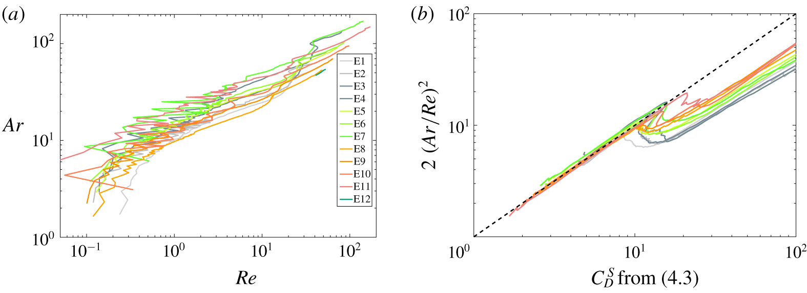
 $Ar^{2}=Re^{2}C_{D}^{S}/2$ for a quasi-steady fall.
In the limit case of a homogeneous fluid ( $1/Fr\rightarrow 0$), in the parameter range
 $Ar\leqslant 50$ associated with
 $Re\leqslant 130$ for which the disk has a stable steady evolution falling broadside-on, the drag coefficient must tend to (Pitter, Pruppacher & Hamielec Reference Pitter, Pruppacher and Hamielec1973; Clift, Grace & Weber Reference Clift, Grace and Weber1978)
 $$\begin{eqnarray}C_{D}^{H}=\frac{64}{\unicode[STIX]{x03C0}Re}(1+0.138Re^{0.792}),\end{eqnarray}$$
valid for  $1.5\lesssim Re\lesssim 133$ and for disks with
 $\unicode[STIX]{x1D712}>1$.
For any stratified fluid ( $Fr$ being finite), in the same parameter range, the drag coefficient can be related to the one in a homogeneous fluid as follows
 $$\begin{eqnarray}C_{D}^{S}=C_{D}^{H}\{1+\unicode[STIX]{x1D6F1}(Fr,Re,{\mathcal{R}},\unicode[STIX]{x1D712},Pr)\},\end{eqnarray}$$
with  $\unicode[STIX]{x1D6F1}$ tending to zero when
 $Fr$ tends to infinity.
In the case of a spherical object evolving in a linearly stratified fluid, one can consider that (2.8) should be written
 $$\begin{eqnarray}C_{D}^{S}=C_{D}^{H}(1+aRe^{p}Fr^{q}),\end{eqnarray}$$
where  $a$,
 $p$ and
 $q$ are constants. These constants can be different, depending on the nature of the stratified fluid through the Schmidt (or Prandtl) number, and on the range of the Reynolds and Froude numbers that are considered, as suggested by previous studies. Indeed, for a sphere at low enough values of the Reynolds number (
 $Re<10$), analytical studies have found power-law dependency with
 $p=1/3$,
 $q=-2/3$ (Zvirin & Chadwick Reference Zvirin and Chadwick1975) or
 $p=1/4$,
 $q=-1/2$ (Candelier et al. Reference Candelier, Mehaddi and Vauquelin2014) is possible. Experimental and numerical studies (Yick et al. Reference Yick, Torres, Peacock and Stocker2009; Kindler et al. Reference Kindler, Khalili and Stocker2010) have matched the values of
 $p=1/2$,
 $q=-1$ and
 $a\simeq 1.9$. As a remark, these studies present the Richardson number
 $Ri=Re/Fr^{2}$ as a more relevant parameter to describe the stratified drag for regimes where buoyancy and viscous forces are at play. Numerical studies (Bayareh et al. Reference Bayareh, Doostmohammadi, Dabiri and Ardekani2013) have found
 $q=-2.8$ and
 $a\simeq 21$ for a droplet rising at fixed values of the Reynolds number (
 $Re=396$ and
 $792$).
3 Experimental and numerical approaches
3.1 Experimental approach
We consider disks of finite thickness (or short-length cylinders) whose densities range between 1020 and  $1025~\text{kg}~\text{m}^{-3}$. Their diameters
 $d$ and heights
 $h$ range from 5 to 20 mm and from 1 to 5 mm, respectively. The corresponding aspect ratios
 $\unicode[STIX]{x1D712}=d/h$ are 3, 6 and 10, determined with an accuracy of 1 %. Disks have been manufactured from cylindrical bars of Nylon and have a density close to (but always larger than) the surrounding salt-stratified fluid. Based on the stratification realized, the parameter
 ${\mathcal{R}}-1$ varies from
 $10^{-2}$ to zero, when the disk reaches its neutral depth. Small imperfections in their design could lead to minor imperfections in the distribution of mass, as discussed in § 4.4.
The disks are released in a large glass tank (50 cm high with a square cross-section of 56 cm width) containing salt-stratified water ( $Sc\simeq 700$). The linearly stratified fluid is obtained using the double-bucket method (Oster Reference Oster1965; Economidou & Hunt Reference Economidou and Hunt2009), the stratification is measured using a microscale conductivity–temperature probe (from PME) displaced using a linear traverse which, after calibration, had a precision of 1 % in conductivity and temperature. Small fluctuations of
 $\unicode[STIX]{x1D70C}(z)$ compared to a linear profile can induce some uncertainties in the estimate of a mean value for
 $N$, of the order of 5 %–10 % on average (see figure 2a for instance), with the specific case of a small value of
 $N$ reaching 40 %. Plastic wrap placed over the top of the tank prevents perturbation induced by convection and evaporation.
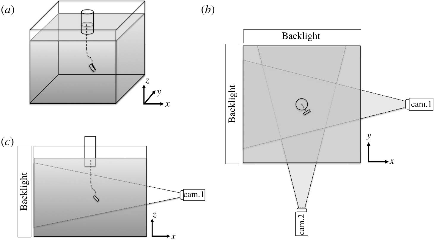
Schematic of the experimental set-up. (a) Overall three-dimensional view, (b) horizontal and (c) side views.

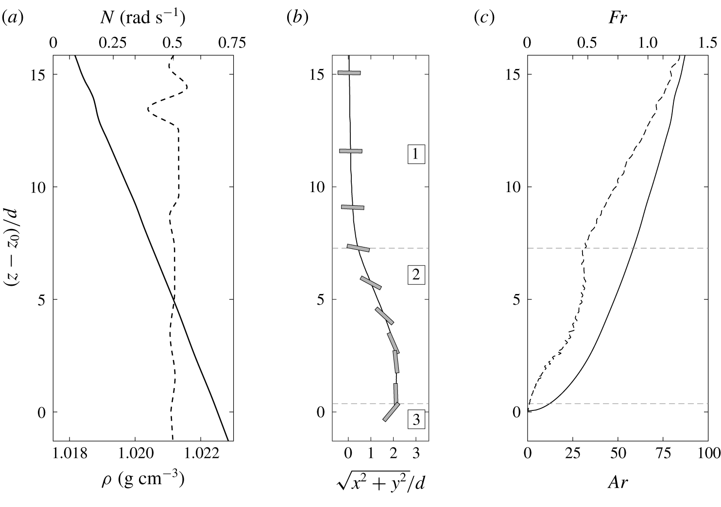
(a) Density (solid) and Brunt–Väisälä frequency (dashed) profiles. (b) Overall settling trajectory for a disk (E5 in table 1) shown in grey reaching its neutrally buoyant depth at  $z_{0}$, where
 $R$ is the horizontal displacement (in the
 $(x,y)$ plane). (c) Archimedes (solid) and Froude (dashed) numbers associated with it. Numbers in (b) indicate the three phases of the trajectory.

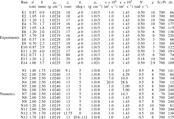
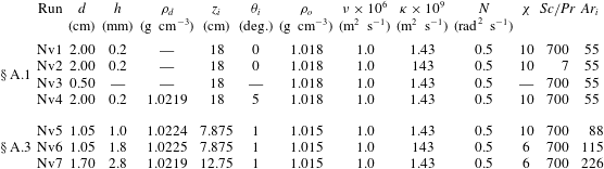
Summary of experiments and numerical simulations (labeled E $X$ and N
 $X$ with
 $X$ being a number, respectively). For experiments,
 $Ar_{i}$ is the value estimated from the start of the trajectory.

The disks are released from a twizzer after being introduced just below the free surface, and into a small cylinder at the centre of the tank, immersed down to  $5$ cm below the free surface, as indicated in figure 1. The main reason for this process is to maintain the disks near the centre of the tank and avoid large flow perturbations in the tank when introducing or removing the twizzer. However, it should be noted that the presence of the cylinder can also induce weak perturbations of the velocity and inclination of the disks when they escape from the cylinder and evolve in the large section of the tank. Below the cylinder, we consider their dynamics unbounded (the distance to the sidewalls is larger than
 $15$ diameters for the largest disk).
A pair of identical cameras ( $1280\times 1024$ pixels) image two perpendicular fields of view of the tank at the sampling frequency between 1 and 5 Hz. Camera
 $1$ images the
 $(y,z)$-plane and camera
 $2$ the
 $(x,y)$-plane, and their fields of view correspond to physical dimensions of approximately
 $32~\text{cm}\times 26~\text{cm}$ in the centre of the tank. This is sufficient to record most of the trajectory without moving the cameras, but the location of the cameras does not permit us to visualize the bottom part of the cylinder, hence we cannot have a recording of the initial conditions of release for the disk orientation or its speed. The cameras are located nearly 2 m away from the centre of the tank and follow the contour of the object that appears dark over a white background, which allows for a recording of the centre of mass of the disk, along with its contour and orientation. Optical set-up allows for a depth of field resolving the three phases of the trajectory, as discussed in § 4.
The stratification can affect the detection of the object due to the vertical gradient of the optical index  $n$ which is proportional to the gradient in density in a stratified fluid. As discussed in Dalziel et al. (Reference Dalziel, Carr, Sveen and Davies2007), the variation in the observed position due to the stratification is proportional to
 $\unicode[STIX]{x1D6FF}z=(L^{2}/2)\unicode[STIX]{x2202}\ln n/\unicode[STIX]{x2202}z$ when observing the object located at a distance
 $L$ from the side of the tank. In our case, the weak and constant density gradient (
 $\unicode[STIX]{x2202}\unicode[STIX]{x1D70C}/\unicode[STIX]{x2202}z\simeq 25~\text{kg}~\text{m}^{-4}$) corresponds to an optical gradient
 $\unicode[STIX]{x2202}n/\unicode[STIX]{x2202}z\simeq 5\times 10^{-3}~\text{m}^{-1}$, that leads to
 $\unicode[STIX]{x1D6FF}z\leqslant 2\times 10^{-4}$ m. When compared to the disk thickness
 $h$,
 $\unicode[STIX]{x1D6FF}z/h\leqslant 0.22$ for the disks used, this indicates an absolute error of
 $0.22h$ in the position of the disk, which is constant over the whole domain. This does not affect the velocity measurements or the estimate of the non-dimensional parameters defined in § 2.
The technique used to extract the three-dimensional dynamics is similar to the approach described in Fernandes et al. (Reference Fernandes, Risso, Ern and Magnaudet2007), and is described in figure 1(b,c). The two cameras are calibrated in three dimensions. For each camera, by imaging a grid at several positions along the optical axis (the grid plane being perpendicular to it), we measure the evolution of the spatial resolution  $\unicode[STIX]{x1D6FD}_{i}$ (
 $i=1$ or
 $2$) from pixel to meter along the optical axis, such that
 $$\begin{eqnarray}\unicode[STIX]{x1D6FD}_{1}(x)=\unicode[STIX]{x1D6FD}_{1}^{0}(1+\unicode[STIX]{x1D716}_{1}x)\quad \text{and}\quad \unicode[STIX]{x1D6FD}_{2}(y)=\unicode[STIX]{x1D6FD}_{2}^{0}(1+\unicode[STIX]{x1D716}_{2}y).\end{eqnarray}$$
As explained before, we neglect the influence of the stratification on the calibration, and  $\unicode[STIX]{x1D6FD}_{i}$ does not depends on
 $z$. In practice, typical values are
 $\unicode[STIX]{x1D6FD}_{i}^{0}\simeq 2.5\times 10^{-4}~\text{m}~\text{pix}^{-1}$, and their variation with position along the optical axis is
 $\unicode[STIX]{x1D716}_{i}\simeq 10^{-2}~\text{m}^{-1}$. The three-dimensional position of the disk is obtained by an iterative process. The position of the disk (centre of mass) is first estimated in each image by using a first guess of the spatial resolution to use (
 $\unicode[STIX]{x1D6FD}_{i}=\unicode[STIX]{x1D6FD}_{i}^{0}$). It allows for a new estimate of the
 $(x,y,z)$-coordinates of the disk, which can be used to update the value of
 $\unicode[STIX]{x1D6FD}_{i}$. The position of the disk is then computed based on these new values of the spatial resolutions for each camera. The iterations end when the norm of the distance between the new position of the disk and the previous estimate is less than
 $10^{-5}~\text{m}$.
A fluorescent dye and UV lightning are used in some cases to visualize the structure of the stratified wake. The disks are immersed in a concentrated solution of fluoresceine with a density matching the density of the top fresh layer of the stratification, before being released in the stratified tank.
For all experimental runs, the parameters are described in table 1.
3.2 Numerical approach
Using the Boussinesq approximation, the equations of motion for viscous, incompressible fluids with variable density in the entire computational domain are written as
 $$\begin{eqnarray}\displaystyle & \displaystyle \unicode[STIX]{x1D735}\boldsymbol{\cdot }\boldsymbol{u}=0, & \displaystyle\end{eqnarray}$$
 $$\begin{eqnarray}\displaystyle & \displaystyle \unicode[STIX]{x1D70C}_{0}\frac{\text{D}\boldsymbol{u}}{\text{D}t}=-\unicode[STIX]{x1D735}p+\unicode[STIX]{x1D707}\unicode[STIX]{x1D6FB}^{2}\boldsymbol{u}+(\unicode[STIX]{x1D70C}-\bar{\unicode[STIX]{x1D70C}})\boldsymbol{g}+\boldsymbol{f}, & \displaystyle\end{eqnarray}$$
where  $t$ is the time,
 $\boldsymbol{u}$ the velocity vector,
 $p$ the hydrodynamic pressure,
 $\boldsymbol{g}$ the gravitational acceleration,
 $\unicode[STIX]{x1D707}$ the dynamic viscosity of the fluid,
 $\unicode[STIX]{x1D70C}_{0}$ the reference fluid density and
 $\bar{\unicode[STIX]{x1D70C}}$ the volumetric average of the density over the entire computational domain. The density
 $\unicode[STIX]{x1D70C}$ can be written as
 $\unicode[STIX]{x1D70C}=\unicode[STIX]{x1D70C}_{f}+\unicode[STIX]{x1D719}(\unicode[STIX]{x1D70C}_{d}-\unicode[STIX]{x1D70C}_{f})$, where
 $\unicode[STIX]{x1D70C}_{f}$ is the fluid density that depends on the fluid temperature or salinity; the indicator function
 $\unicode[STIX]{x1D719}$, which represents the volume fraction of grid cells occupied by the solid disk, is a phase indicator to identify the disk and liquid phases with
 $\unicode[STIX]{x1D719}=1$ inside the disk and
 $\unicode[STIX]{x1D719}=0$ inside the fluid domain. The body force
 $\boldsymbol{f}$ in the momentum equation, equation (3.3), accounts for the solid–fluid interaction by using a distributed Lagrange multiplier method, which has been extensively employed to study the settling of rigid, general-shaped particles in both homogeneous fluids and stratified fluids (Ardekani, Dabiri & Rangel Reference Ardekani, Dabiri and Rangel2008; Doostmohammadi & Ardekani Reference Doostmohammadi and Ardekani2013, Reference Doostmohammadi and Ardekani2014, Reference Doostmohammadi and Ardekani2015; Doostmohammadi et al. Reference Doostmohammadi, Dabiri and Ardekani2014). The disk is impermeable to the stratifying agent and the temporal evolution of the density field is governed by a convection–diffusion process described by
 $$\begin{eqnarray}\frac{\text{D}\unicode[STIX]{x1D70C}}{\text{D}t}=\unicode[STIX]{x1D705}\unicode[STIX]{x1D6FB}^{2}\unicode[STIX]{x1D70C},\end{eqnarray}$$
where  $\unicode[STIX]{x1D705}$ is the diffusivity of the stratifying agent. Equations (3.2)–(3.4) are discretized using a finite volume method on non-uniform fixed Cartesian staggered grids. The time discretization is obtained using a first-order Euler method. The convection and diffusion terms in both (3.3) and (3.4) are solved using the QUICK (quadratic upstream interpolation for convective kinetics) and central-difference schemes (Leonard Reference Leonard1979), respectively. The disk is initially placed at the centre of the
 $(x,y)$ plane and settles from location
 $z_{i}$, at which the fluid density is
 $\unicode[STIX]{x1D70C}_{0}$, with an initial inclination
 $\unicode[STIX]{x1D703}_{i}$ with respect to the horizontal direction and no initial velocity. The no-slip boundary condition is enforced on the disk surface. The initial fluid density linearly varies with depth
 $\unicode[STIX]{x1D70C}_{f}=\unicode[STIX]{x1D70C}_{0}+\unicode[STIX]{x1D6FE}(z-z_{i})$, where
 $\unicode[STIX]{x1D6FE}$ is the vertical density gradient and
 $z$ is the vertical component of spatial coordinates. The periodic boundary conditions for density and velocity components are used on side boundaries of the rectangular computational domain. The boundary conditions for density and velocity on the top and bottom boundaries are defined as
 $(\unicode[STIX]{x2202}\unicode[STIX]{x1D70C}/\unicode[STIX]{x2202}z)=\unicode[STIX]{x1D6FE}$ and
 $(\unicode[STIX]{x2202}\boldsymbol{u}/\unicode[STIX]{x2202}z)=0$, respectively.
We would like to highlight that stratified flows develop thin boundary layers at high Prandtl numbers that are computationally expensive to resolve. In this work, we use a horizontal and vertical resolution of 128 grid points per diameter for all numerical studies. While the density distribution in the jet would not be resolved with grid sizes below  $d/128$, the settling velocity and drag coefficient would be still accurate for grid sizes as coarse as
 $d/64$. While the grid resolution used in this manuscript is not enough to resolve the thickness of a steady jet, the disk orientation instability occurs well before the steady jet develops; and during this transient behaviour studied in the present work, the jet thickness is wider than the theoretical estimation for the steady jet (see § A.1 for details). Consequently, the settling velocity and the orientation of the disk can be computed accurately, in agreement with the experiment. Finally, increasing the value of
 $N$ generates a narrower jet, and requires a finer resolution, leading to computationally expensive simulations (Towns et al. Reference Towns, Cockerill, Dahan, Foster, Gaither, Grimshaw, Hazlewood, Lathrop, Lifka and Peterson2014).
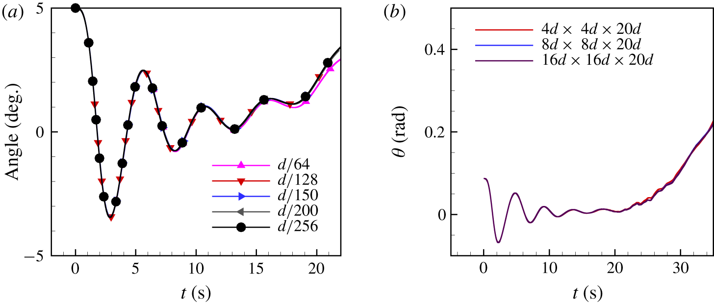
The size of the computational domain is  $4d\times 4d\times 25d$, this lateral extent does not modify the onset of the instability compared to larger domains (see § A.2).
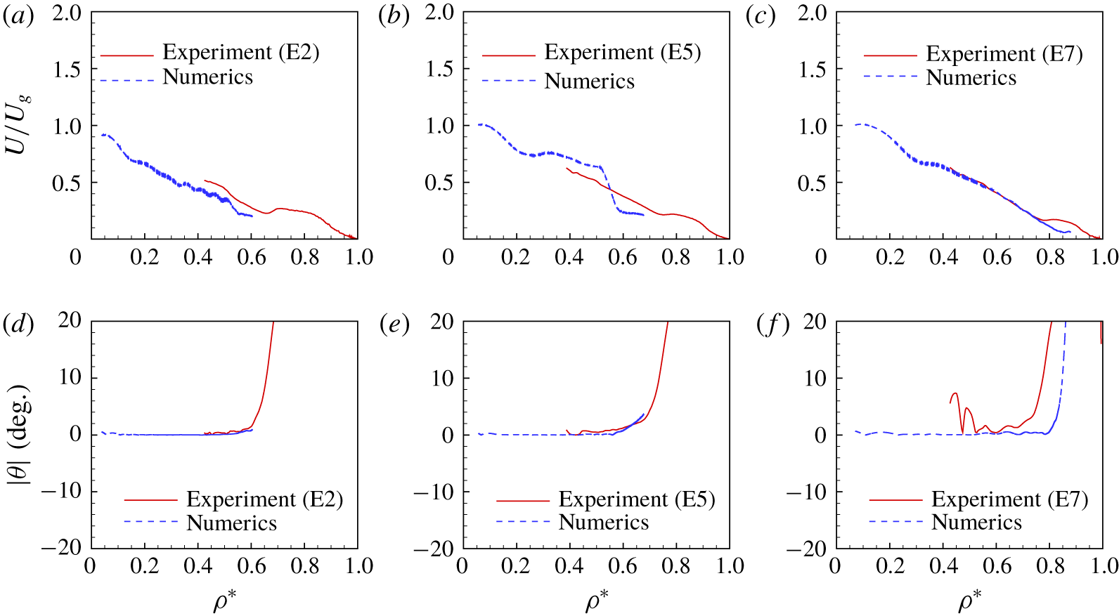
For all numerical runs, the parameters are described in table 1. Additional runs for direct comparison with experiments are also presented in § A.3.
4 Results
We first present the overall generic trajectory for a disk settling in a linearly stratified fluid, before investigating more thoroughly the three distinct phases. As mentioned in the introduction, we limit ourselves to low enough Reynolds numbers so that the orientation of the disk in a homogeneous fluid would remain broadside-on, typically  $Re\leqslant 100$ (Willmarth et al. Reference Willmarth, Hawk and Harvey1964).
4.1 Overall trajectory of a settling disk
The overall trajectory of a settling disk is shown in figure 2. Figure 2(a) indicates the density stratification  $\unicode[STIX]{x1D70C}(z)$ and the corresponding profile of
 $N(z)$, which can be considered nearly constant with
 $N\simeq 0.5~\text{rad}~\text{s}^{-1}$ over the entire column in this case. Figure 2(b) displays the trajectory of the centre of the disk, along with the disk orientation (grey rectangle). Finally, figure 2(c) provides the corresponding evolution of the Archimedes and Froude numbers during the settling process.
Three regimes for the settling dynamics have been identified before the disk reaches its neutrally buoyant level. First, the disk experiences a quasi-steady phase when the stratification enhances the steady drag experienced by the disk falling broadside-on. We identify this first phase based on the inclination of the disk ( $\unicode[STIX]{x1D703}\simeq 0$). Along this phase, we still have a variation of the velocity and non-dimensional parameters with
 $z$, as can be noticed in figure 2(c). Then, there is a change of stability for the disk orientation (from broadside-on to edgewise) when the value of the disks’ velocities become ‘sufficiently’ small. Similarly to phase 1, we identify the start of this second phase based on the inclination of the disk, when it becomes non-zero (we set an arbitrary threshold
 $\unicode[STIX]{x1D703}>5^{\circ }$). Finally, the last phase corresponds to the disk settling edgewise until stopping at its gravitational equilibrium level
 $z_{0}$, defined by
 $\unicode[STIX]{x1D70C}(z_{0})=\unicode[STIX]{x1D70C}_{d}$. At the end of its settling, it returns towards a horizontal orientation. We identify the start of this final phase based on
 $\unicode[STIX]{x1D703}\simeq 90^{\circ }$ or by the maximum value reached along the trajectory, some disks ending their trajectory without completing the whole phase 2.
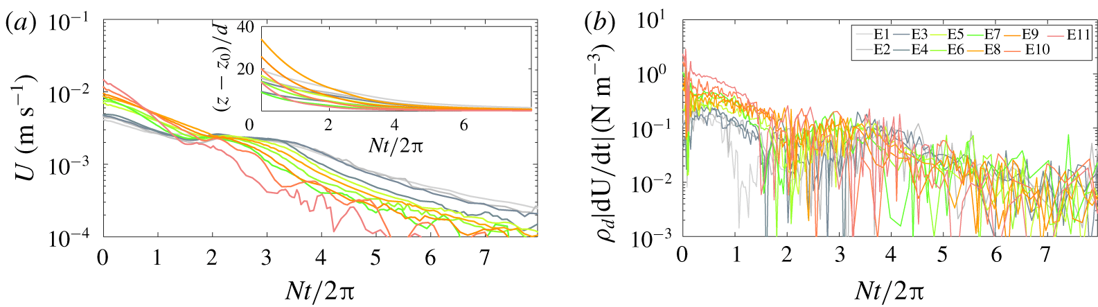
Temporal evolution for many experimental disks of (a) the vertical velocity  $U$ and position
 $z$, along with (b) the acceleration force
 $\unicode[STIX]{x1D70C}_{d}|\text{d}U/\text{d}t|$. See table 1 for details on parameters.

It should be noted that, for both the experimental and numerical cases studied, the three phases of the dynamics occur in a plane (no helicoidal motion is observed). Furthermore, for a given experiment or numerical simulation, all the non-dimensional parameters are not independent, more specifically the Reynolds  $Re$ and Froude
 $Fr$ numbers follow this relationship
 $Re/Fr=Nd^{2}/\unicode[STIX]{x1D708}$ which is constant for a single experiment;
 $N$ and
 $d$ are different for different experiments.
4.2 Phase 1: broadside-on settling
We consider the part of the trajectory with broadside-on settling, corresponding to phase 1 in figure 2(b). We first study the assumption of quasi-steady fall for the disk broadside-on, by comparing the importance of acceleration with drag and buoyancy forces. As can be seen in figure 3(a), it is for non-dimensional times  $Nt/2\unicode[STIX]{x03C0}$ smaller than
 $2$ that the velocity of the disk changes the most. This is confirmed in figure 3(b) where we measure
 $\text{d}U/\text{d}t$ to be of the order of
 ${\sim}10^{-3}~\text{m}~\text{s}^{-2}$ at most. For the problem considered, buoyancy forces are of the order of
 $10^{2}~\text{N}~\text{m}^{-3}$ whereas an estimate of the stratified drag coefficient is at least as large as in homogeneous case (
 $C_{D}^{H}\sim 1$ for
 $Re\in [10,100]$), leading to
 $\unicode[STIX]{x1D70C}(z)C_{D}^{S}U^{2}/2h\sim 10^{2}~\text{N}~\text{m}^{-3}$ in our experiments. If we compare the values of these terms of opposite signs on the right-hand side of (2.1) with acceleration forces which are of order
 $1~\text{N}~\text{m}^{-3}$, this confirms our assumption of quasi-steady fall where buoyancy and drag forces are the dominant forces, and the small differences between the two is associated with small acceleration forces. Similar results have been obtained from the numerical simulations, although not shown here.
We seek for a generic expression for the stratified drag coefficient of a disk, thus we consider the trajectories of many disks of various aspect ratios and diameters ( $d$,
 $h$ and
 $\unicode[STIX]{x1D712}$ varied), evolving in different stratified environments (
 $N$,
 $\unicode[STIX]{x1D708}$ and
 $\unicode[STIX]{x1D705}$ changed). The parameters for each experimental or numerical run are listed in table 1.
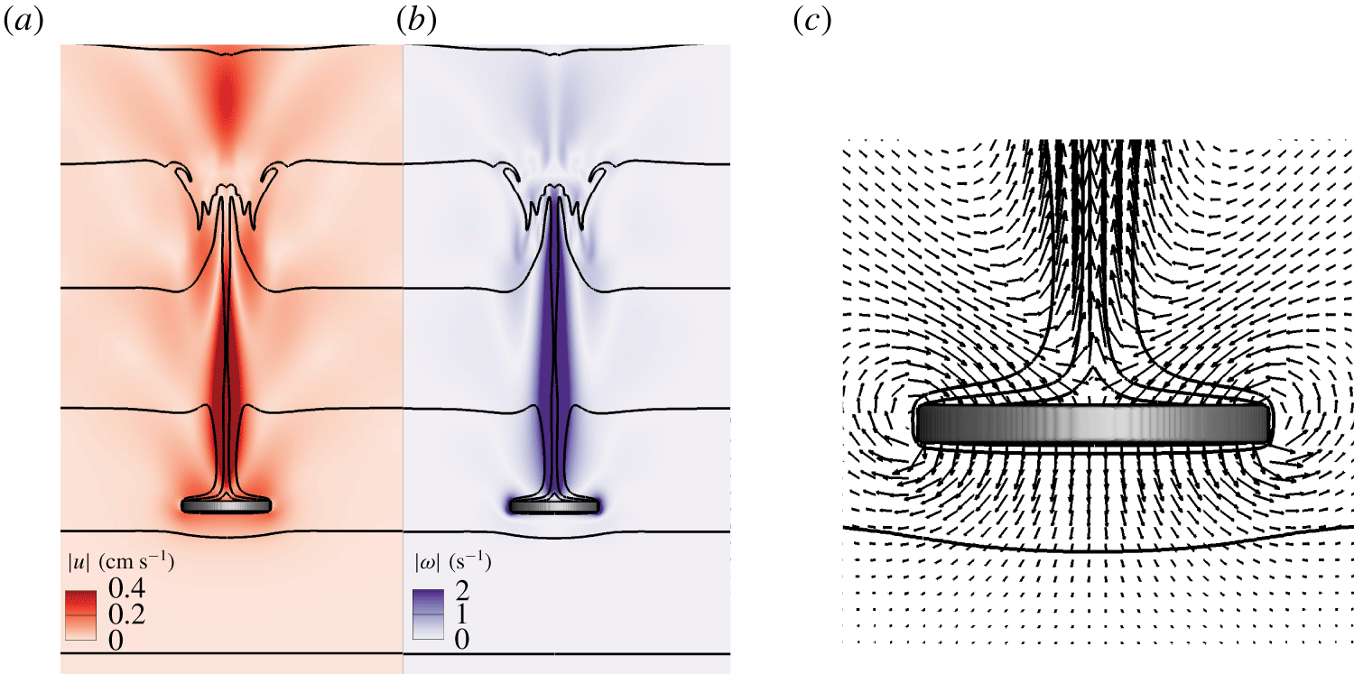
The numerical simulations provide a more complete description of the flow around the disk in this quasi-steady phase. Here, we present results associated with a steady broadside-on settling for disks initially released with no velocity and  $\unicode[STIX]{x1D703}_{i}=0$ (runs N
 $10$ and
 $11$). As the disk settles across a linearly stratified fluid, lighter fluid is drawn down from its original position. Visible in figure 4 is that the vertical displacement of isopycnals, denoted as
 $\unicode[STIX]{x1D6E4}=(z_{\unicode[STIX]{x1D70C}}(t)-z_{\unicode[STIX]{x1D70C}}(0))/d$, can be as large as 3. Similar observations have been reported for a sphere moving downward in a salt-stratified fluid (
 $Sc=700$), where isopycnals are displaced for a large extent (Hanazaki et al. Reference Hanazaki, Konishi and Okamura2009b; Doostmohammadi et al. Reference Doostmohammadi, Dabiri and Ardekani2014; Hanazaki et al. Reference Hanazaki, Nakamura and Yoshikawa2015). One can notice a bell-shape structure along the jet axis in the far wake, as described in Hanazaki et al. (Reference Hanazaki, Nakamura and Yoshikawa2015). This structure is related to internal waves generated in the wake of the settling object. Internal waves generated upon settling can affect phase 3, as discussed later. Nevertheless, during the quasi-steady phase, since the flow structure around the disk remains axisymmetric (see figure 4a,b), the disk settles under the broadside-on configuration.
Colour maps of (a) velocity  $|\boldsymbol{u}|$ and (b) vorticity
 $|\unicode[STIX]{x1D74E}|$ fields for run N
 $12$. (c) Zoom on the velocity vector field around the disk. Black solid lines are isopycnals for
 $\unicode[STIX]{x1D70C}$ equals
 $1017.5$ to
 $1020.6~\text{kg}~\text{cm}^{-3}$ by steps of
 $0.588~\text{kg}~\text{cm}^{-3}$. In (c), isopycnals with
 $\unicode[STIX]{x1D70C}=1017.5~\text{kg}~\text{cm}^{-3}$ and
 $\unicode[STIX]{x1D70C}=1020.6~\text{kg}~\text{cm}^{-3}$ are not visible. The images correspond to
 $U=0.18~\text{cm}~\text{s}^{-1}$.

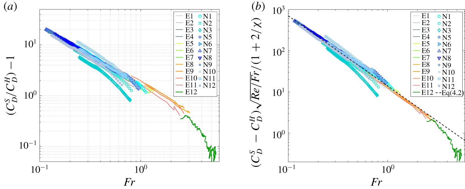
Stratified drag coefficient  $C_{D}^{S}$ minus the homogeneous drag coefficient
 $C_{D}^{H}$ in (a), and normalized by a function of the aspect ratio
 $\unicode[STIX]{x1D712}$ in (b), as a function of the Froude numbers during quasi-steady settling for trajectories identified in figure 3(c). Symbols correspond to numerical simulations. The dashed line in (b) is the fit of the power law as given in (4.3).

Based on the disk velocity and the background fluid density profiles along the trajectories in figure 3, we can compute the stratified drag coefficient  $C_{D}^{S}$ using (2.2). To compare it to the homogeneous case and seek an expression similar to (2.8), we display
 $C_{D}^{S}/C_{D}^{H}-1$ in figure 5(a) as a function of the Froude number. The same quantity is also obtained from numerical runs. Although the observations seem to exhibit similar trends in figure 5(a), the results do not all collapse onto a unique curve and we seek a better description of the normalized drag coefficient with the parameters. Yick et al. (Reference Yick, Torres, Peacock and Stocker2009) suggest that the origin of the added drag on a settling sphere in a linearly stratified fluid is due to the extra buoyancy force generated by a spherical shell of light fluid around the sphere, entrained by viscosity over some distance while settling. Thus we can express the extra stratified drag normalized with the drag for a homogeneous fluid as a buoyancy force corresponding to the fluid displaced by the object,
 $$\begin{eqnarray}\frac{C_{D}^{S}}{C_{D}^{H}}-1\simeq \frac{\unicode[STIX]{x0394}\unicode[STIX]{x1D70C}gV}{\frac{1}{2}C_{D}^{H}\unicode[STIX]{x1D70C}U^{2}S},\end{eqnarray}$$
with  $S$ the apparent section of the object,
 $V$ the volume of light fluid displaced and
 $\unicode[STIX]{x0394}\unicode[STIX]{x1D70C}$ its density difference with the fluid at the depth of the object. When applied to the disk geometry, we can consider that a shell of light fluid of width
 $\unicode[STIX]{x1D6FF}$ has a volume
 $V$ which scales like
 $(\unicode[STIX]{x03C0}/2)d^{2}\unicode[STIX]{x1D6FF}(1+2/\unicode[STIX]{x1D712})$ when
 $\unicode[STIX]{x1D6FF}/d\ll 1$, compared to the case of the sphere with
 $V$ that scales like
 $\unicode[STIX]{x03C0}d^{2}\unicode[STIX]{x1D6FF}$. Observations from numerical simulations zoomed on the proximity of the disk, as shown in figure 4(c), confirm that a thin shell of light fluid moves with the object (see also figure 7). For both geometries,
 $S$ scales like
 $(\unicode[STIX]{x03C0}/4)d^{2}$. The light fluid composing the shell has been displaced over some distance
 $\unicode[STIX]{x1D6E4}d$, as already discussed when presenting the numerical results in figure 4, and we can estimate its density based on the density gradient such that
 $\unicode[STIX]{x0394}\unicode[STIX]{x1D70C}=\unicode[STIX]{x1D6E4}d(N^{2}\unicode[STIX]{x1D70C}/g)$. In the end, the extra drag due to the stratification normalized with the homogeneous fluid becomes
 $$\begin{eqnarray}\frac{C_{D}^{S}}{C_{D}^{H}}-1\simeq \frac{1}{C_{D}^{H}}\frac{\unicode[STIX]{x1D6E4}}{Fr^{2}}\frac{\unicode[STIX]{x1D6FF}}{d}\left(1+\frac{2}{\unicode[STIX]{x1D712}}\right),\end{eqnarray}$$
and we must consider proper scalings for  $\unicode[STIX]{x1D6FF}$ and
 $\unicode[STIX]{x1D6E4}$.
It has been shown in previous studies (Yick et al. Reference Yick, Torres, Peacock and Stocker2009; Hanazaki et al. Reference Hanazaki, Nakamura and Yoshikawa2015) that the width  $\unicode[STIX]{x1D6FF}$ of the light fluid shell entrained by viscous effects should scale like
 $\sqrt{\unicode[STIX]{x1D708}/N}$, which leads to
 $\unicode[STIX]{x1D6FF}/d\sim \sqrt{Fr/Re}$. It should be noted that, for a single experiment,
 $\unicode[STIX]{x1D6FF}/d$ is constant, but depends on the fluid and disk properties. The scaling law for the vertical entrainment of fluid
 $\unicode[STIX]{x1D6E4}$ depends on the Froude number, but is not universal. Typically, one considers
 $\unicode[STIX]{x1D6E4}\sim Fr^{\unicode[STIX]{x1D6FC}}$, and the constant
 $\unicode[STIX]{x1D6FC}$ depends on the range of values encountered for
 $Re$. Observations led to
 $\unicode[STIX]{x1D6FC}=1/2$ for a sphere when
 $Re<1$ (Yick et al. Reference Yick, Torres, Peacock and Stocker2009) and
 $\unicode[STIX]{x1D6FC}=1$ for spheres (Hanazaki et al. Reference Hanazaki, Nakamura and Yoshikawa2015) with
 $Re\geqslant 200$ and
 $Fr\geqslant 1$, or for cylinders with
 $Re\sim O(10^{3})$ (Higginson, Dalziel & Linden Reference Higginson, Dalziel and Linden2003). As displayed in figure 5(b), by looking at
 $(C_{D}^{S}-C_{D}^{H})\sqrt{Re/Fr}/(1+2/\unicode[STIX]{x1D712})$ we seek a rescaled evolution of the drag coefficient that depends on
 $Fr$ only, and the data nicely collapse into a single curve that can be fitted as
 $$\begin{eqnarray}C_{D}^{S}=C_{D}^{H}\left[1+\frac{\boldsymbol{a}}{C_{D}^{H}}\left(1+\frac{2}{\unicode[STIX]{x1D712}}\right)\sqrt{\frac{Fr}{Re}}\,Fr^{\boldsymbol{q}}\right],\end{eqnarray}$$
with the fitting parameters,  $a=14\pm 2$ and
 $q=-1.7\pm 0.1$. This validates the discussion above with a value of
 $\unicode[STIX]{x1D6FC}=0.3\pm 0.1$ for the case of a disk.
In the end, the drag model in (4.3) is consistent with (2.8), with only  $\unicode[STIX]{x1D712}$,
 $Re$ and
 $Fr$ playing a key part in this parameter space for values of
 $Re\in [5,130]$,
 $Fr\in [0.1,3]$,
 $Pr\in [70,700]$ and
 $\unicode[STIX]{x1D712}\in [3,10]$. One must notice the good agreement for both the experimental and numerical results with the same modelling approach. These results can be furthermore validated by investigating the relation between the Archimedes and Reynolds numbers. As mentioned in § 2, one expects
 $2(Ar/Re)^{2}=C_{D}^{S}$ in a quasi-steady regime. If we compare
 $2(Ar/Re)^{2}$ to the expression in (4.3), we do find a good correlation for phase 1 (cf. figure 16b in appendix B).
Compared to the known results for the sphere (Yick et al. Reference Yick, Torres, Peacock and Stocker2009) in the same range of parameters ( $C_{D}^{S}/C_{D}^{H}-1\sim Re^{1/2}Fr^{-1}$), here we find
 $C_{D}^{S}/C_{D}^{H}-1\sim (1+2/\unicode[STIX]{x1D712})Re^{1/2}Fr^{-1.2}$ if we consider the drag on the disk to be
 $C_{D}^{H}\sim Re^{-1}$. This indicates that the disk is more strongly affected by the stratification (stronger added drag) than a sphere of similar diameter. We will come back on the implication of this aspect (cf. table 2) in the conclusion.
4.3 Phase 2: instability of the broadside-on settling
When the vertical velocity of the disk decreases, there is a change of stability for the disk orientation from broadside-on to edgewise settling, this part of the trajectory corresponds to phase 2 in figure 2(b). As we will see, this transition in the orientation of the disk from  $0$ to
 $\unicode[STIX]{x03C0}/2$ seems to be a robust feature, for values of the Reynolds number in the range 10–50, and of the Froude number in the range 0.1–2 and various stratified environments. It should be noted that some of the disks do not reach the
 $\unicode[STIX]{x03C0}/2$-orientation before initiation of phase 3 (when the disk reaches its equilibrium depth). Furthermore, although not shown here, it is important to stress that the dynamics of phase 2 takes place in a plane, no helicoidal motion has been observed in experiments or numerics.
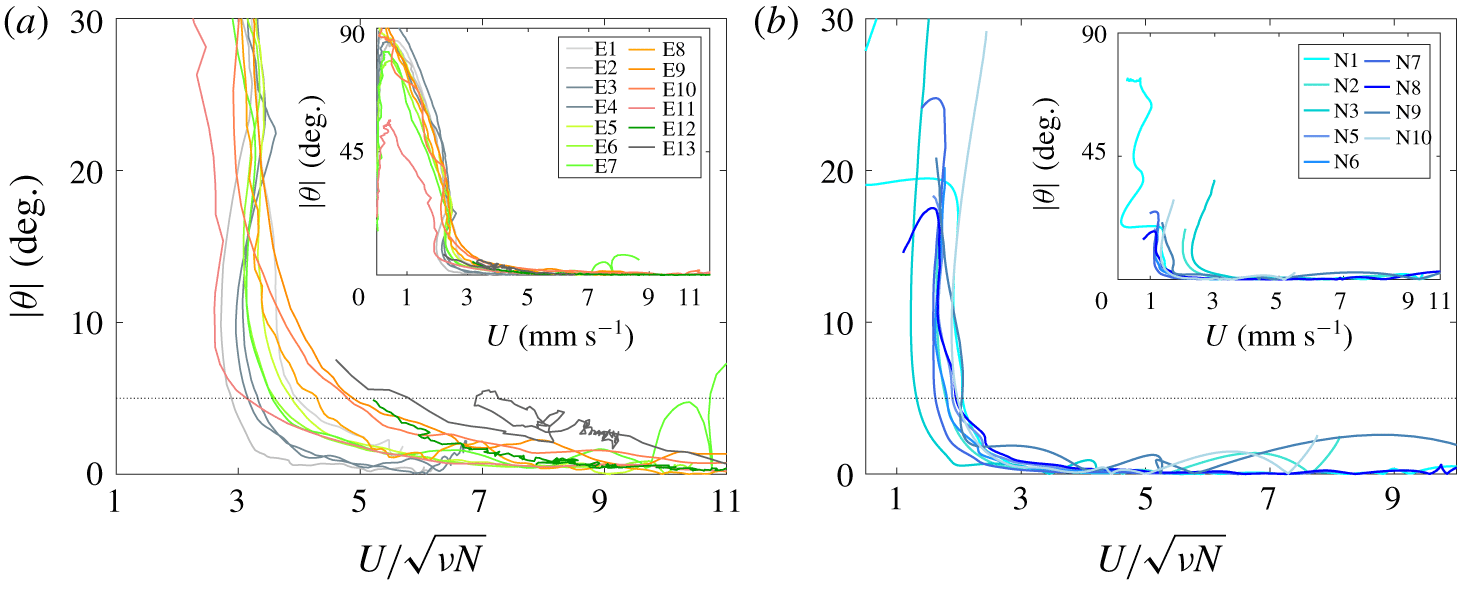
Orientation angle  $\unicode[STIX]{x1D703}$ as a function of the vertical velocity
 $U$ normalized by
 $\sqrt{\unicode[STIX]{x1D708}N}$ for (a) experimental and (b) numerical runs studying the change of stability. Insets show
 $\unicode[STIX]{x1D703}$ versus
 $U$ over the whole trajectory.

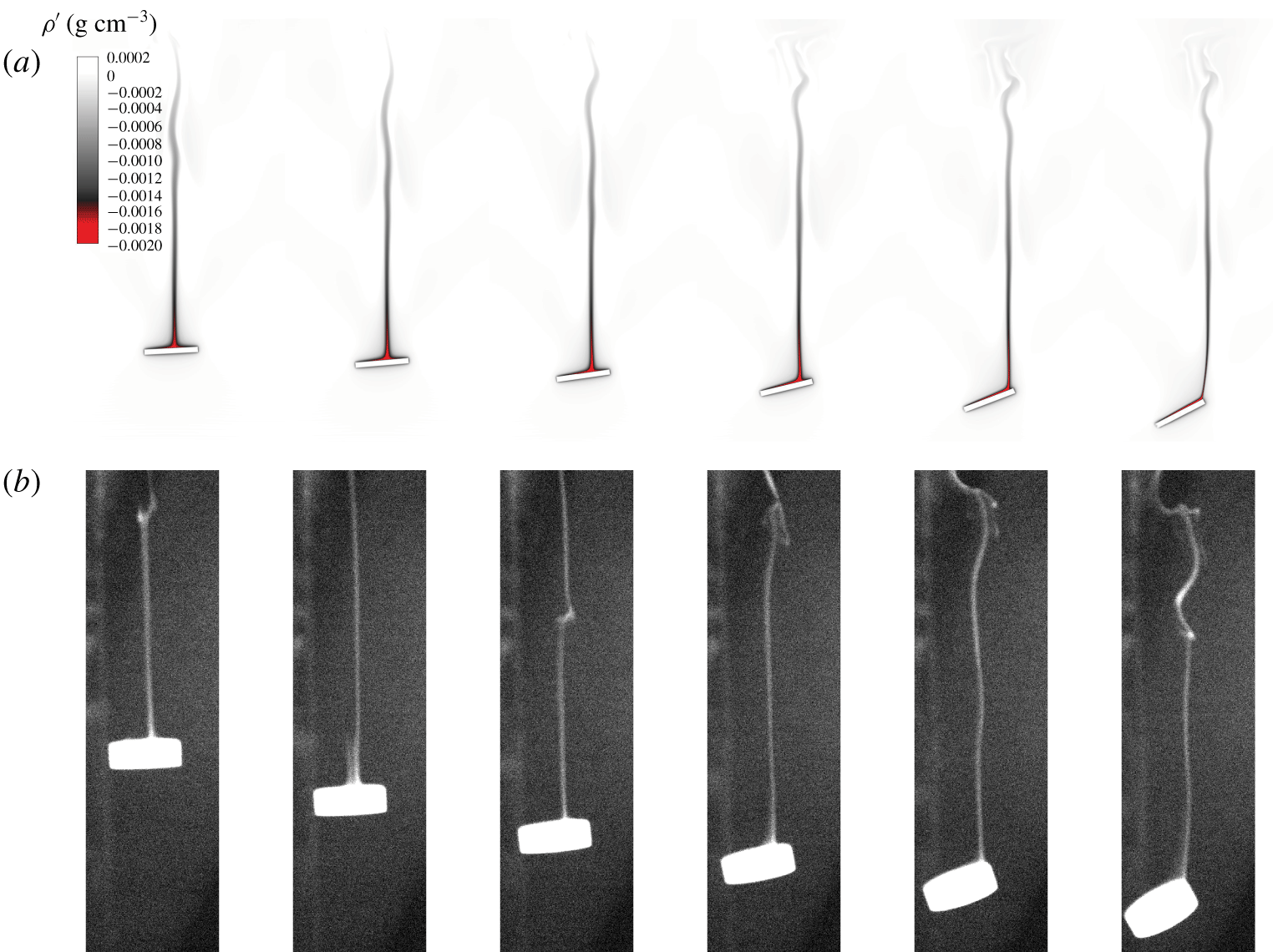
Examples of wake visualizations during phase 2 in experiments and numerics, the parameters chosen for each run are different. Maps of (a) density variations  $\unicode[STIX]{x1D70C}^{\star }=\unicode[STIX]{x1D70C}-\unicode[STIX]{x1D70C}_{f}$ for the numerical simulation (run N
 $10$), and (b) fluorescent dye for the experiment (run E
 $14$). At the first frame,
 $Re\simeq 40$ and
 $Fr\simeq 0.75$ for experiments and
 $Re\simeq 17$ and
 $Fr\simeq 0.23$ for numerics; each frame is separated by
 $\unicode[STIX]{x0394}t=2~\text{s}$, i.e.
 $N\unicode[STIX]{x0394}t=1$.

Figure 6 displays the evolution of the orientation as a function the vertical velocity (insets) and of a non-dimensional velocity  $U/\sqrt{\unicode[STIX]{x1D708}N}$ for both experimental and numerical disks. One should notice that the dynamics of all disks starts in phase 1, corresponding to a large velocity with
 $\unicode[STIX]{x1D703}\sim 0$, then its rotation starts (phase 2) at some lower velocity where
 $\unicode[STIX]{x1D703}$ suddenly increases; each trajectory in figure 6 reads from right to left. In the numerical simulations displayed (runs N
 $1$ to
 $10$), it should be noted that we set the initial inclination at
 $\unicode[STIX]{x1D703}_{i}=5^{\circ }$. For numerical simulations of a single disk released with
 $\unicode[STIX]{x1D703}_{i}=0$ (runs N
 $11$ to
 $12$, used in phase 1), the analysis shows that the orientation angle of these disks remains constant at
 $\unicode[STIX]{x1D703}\simeq 0$ during the whole settling motion computed.
One can notice that all disks start rotating below a threshold non-dimensional velocity of  $3.9\pm 1.1$ for experimental runs (figure 6a), and of
 $1.8\pm 0.2$ for numerical runs (figure 6b). Since there is some dispersion of the values for the non-dimensional velocity at which the angle starts to increase, we defined the threshold value for
 $U_{c}$ to be the velocity when
 $\unicode[STIX]{x1D703}=5^{\circ }$. We also denote
 $\unicode[STIX]{x1D70C}_{c}$ as the density of the fluid for this instant in the trajectory. We did not find such a collapse of the evolution of
 $\unicode[STIX]{x1D703}$ when searching for the influence of
 $Pr$,
 $Ar$ or
 $Fr$ on this threshold. We discuss the dynamics of the change of stability in more detail in § 5.
Finally, we emphasize that the dynamics of phase 2 is associated with a complicated process coupling the stratified flow structure in the wake of a freely rotating object of anisotropic shape. However, some important features can be identified in the experiments and numerical simulations. In figure 7, we present snapshots of the stratified wake visualized using dye for experiments, and by tracking the magnitude of the density perturbations for the numerics (see colour map in figure 7a), for two different runs. Similarly to the case of a sphere studied in Hanazaki et al. (Reference Hanazaki, Kashimoto and Okamura2009a), the stable wake of a moving object in a stratified fluid is mainly composed of a narrow vertical jet. This jet is generated by the up-going fluid that is lighter than its surroundings, initially entrained by viscosity within a thin shell around the object, as already discussed in § 4.2. When the disk starts to rotate, this narrow jet slowly drifts from the centre of the back face of the disk, inducing a torque on the disk that amplifies the rotation. Both the experimental and the numerical approaches are able to obtain this dynamics with very similar trends between the two.
This change of the stratified wake behind the disk could depend on its aspect ratio, its settling speed, its orientation and the stratified environment. We discuss the stability and the dynamics of the rotation in § 5, but we anticipate that more studies are needed to characterize the vertical dynamics of a tilted disk, when its orientation is fixed since it is impossible to discriminate what effect occurs first, the modification of the orientation of the disk or the position of the jet (if any order is applicable).
4.4 Phase 3: reaching a neutrally buoyant depth
Finally, when the disk ends up settling edgewise and gets close to its neutrally buoyant depth  $z_{0}$, it returns to a nearly horizontal orientation, which we characterize by an equilibrium angle
 $\unicode[STIX]{x1D703}(z_{0})=\unicode[STIX]{x1D6FC}$. In the case of a perfectly designed disk, with the centre of buoyancy at the centre of the geometry, one expects
 $\unicode[STIX]{x1D6FC}=0$. However, as described in appendix C, minor imperfections in the distribution of mass (or in the shape equivalently) can lead to non-zero equilibrium inclination angles. We investigate the impact of this observation in § 5.4.
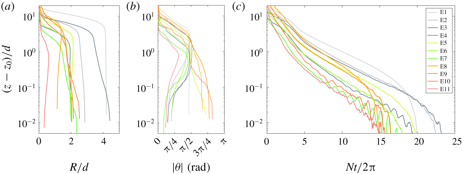
This last phase is associated with a nearly zero horizontal drift while rotating, as shown in figure 8(a,b), although the spatial resolution might not be sufficient to draw any conclusions. Similarly to the change of stability at the initiation of phase 2, the rotation from a nearly vertical disk to the equilibrium angle seems to be similar for all disks, as shown in figure 6(b), with a clear change of stability from vertical to horizontal. It is interesting to notice that this rotation can be towards 0 or  $\unicode[STIX]{x03C0}$, suggesting that the initiation of phase 2 of the trajectory is not automatically correlated with the imperfection in the distribution of mass (heavy face can be up or down).
(a) The settling trajectories, (b) the orientation angle and (c) the temporal evolution of the vertical position in logarithmic scale for experimental disks to emphasize phase 3.

The temporal evolution during this last phase is very slow compared to phases 1 and 2, with values of the Reynolds number smaller than  $1$. Numerical simulations of this last phase have not been obtained due to very long computational times. As shown in figure 8(c), most disks reach
 $z_{0}$ smoothly. However, some disks oscillate around the equilibrium position
 $z_{0}$. We observed that all the oscillatory cases are associated with a maximum value for the Reynolds number larger than
 $80$, whereas the maximum values of the Froude number could be smaller or larger than
 $1$. These oscillations are due to internal motion of the fluid (internal waves) generated while releasing the disks or during phase 1, as mentioned in § 4.2, since the frequency of this oscillatory motion is near
 $N$. This is similar to observations made for a sphere settling in a linearly stratified fluid from the surface down to a neutrally buoyant depth
 $z_{0}$ (Biró et al. Reference Biró, Gábor Szabó, Gyüre, Jánosi and Tél2008a), where oscillations around
 $z_{0}$ were observed due to internal waves generated by the wake of the settling body, with initial values of the Reynolds number larger than
 $300$.
5 Discussion on the change of stability of the disk orientation
Based on the experimental and numerical results, several points have been identified in the dynamics of a disk in a linearly stratified fluid with various values for the disk and the fluid properties. First of all, the broadside-on settling at moderate Reynolds number ( $Re>10$) is a stable regime for the disk, for Froude numbers larger than 0.1–1 (depending on the value of the Reynolds number). An instability of the broadside-on settling occurs when the non-dimensional velocity
 $U/\sqrt{\unicode[STIX]{x1D708}N}$ becomes smaller than a threshold value (
 $3.9\pm 1.1$ for experiments and
 $1.8\pm 0.2$ for numerics) leading to the edgewise orientation as a new stable orientation, as shown in figure 6. The threshold for experimental and numerical runs have similar values and the instability in orientation is a robust effect of the stratified environment. However, more information can be provided on the disk dynamics and on the origin of the instability, in order to help modelling this instability. We provide here complementary analyses and results by means of numerical simulations to investigate the change of stability of the orientation of the disk.
5.1 Possible orientations for settling
We first focus on the perfectly balanced disk, and discuss the stability of a specific orientation for settling. As described in § 4.2, we have investigated the stability of the broadside-on settling in a linearly stratified fluid for a perfectly balanced disk. All numerical simulations initiated in a fluid at rest, with no velocity ( $U_{i}=0$) and no tilt for the disk (
 $\unicode[STIX]{x1D703}_{i}=0$), lead to a steady vertical settling for the disk. More precisely, during the same time (
 $Nt/2\unicode[STIX]{x03C0}<3$), variations in the orientation angle remain very weak (
 $\unicode[STIX]{x1D703}<10^{-1}~\text{rad}$), and have a very weak tendency to increase. Hence, we conclude that the settling dynamics in a linearly stratified fluid at rest, with an initial orientation
 $\unicode[STIX]{x1D703}_{i}=0$, can be considered an equilibrium position for the disk. A complementary study investigates the stability of the edgewise settling. Numerical simulations of a disk (similar to run N
 $11$) are realized with a initial orientation
 $\unicode[STIX]{x1D703}_{i}\simeq \unicode[STIX]{x03C0}/2$ and different values of the viscosity. In a homogenous fluid, the disk eventually settles under the broadside-on configuration regardless of the initial release condition. When settling in a linearly stratified fluid, a disk with an initial orientation
 $\unicode[STIX]{x1D703}_{i}=85^{\circ }$ can be stable at low values of the Reynolds and Froude numbers with
 $Re\leqslant 11.2$,
 $Fr\leqslant 1.14$ (
 $\unicode[STIX]{x1D708}=10^{-5}~\text{m}^{2}~\text{s}^{-1}$), and is unstable for larger values tested such as
 $Re=304$,
 $Fr=3.1$ (
 $\unicode[STIX]{x1D708}=10^{-6}~\text{m}^{2}~\text{s}^{-1}$). This is in good agreement with the experimental observations. Here again we can conclude that the settling dynamics in a linearly stratified fluid at rest, with an initial orientation
 $\unicode[STIX]{x1D703}_{i}=\unicode[STIX]{x03C0}/2$, can be considered an equilibrium position for the disk at low enough velocities. We must now study the stability of these equilibrium positions.
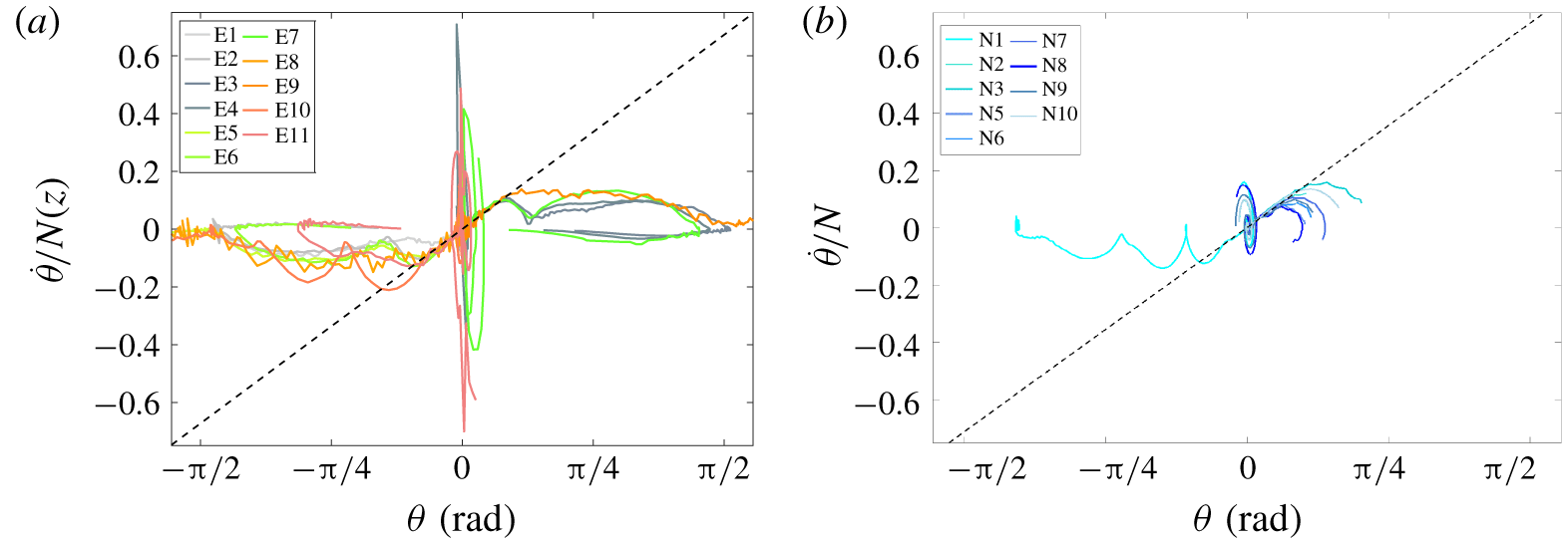
Phase diagram ( $\unicode[STIX]{x1D703},\dot{\unicode[STIX]{x1D703}}/N$) of the orientation for the (a) experimental and (b) numerical runs. The dashed black line has a slope
 $\unicode[STIX]{x1D70E}_{m}/2\unicode[STIX]{x03C0}$, as defined in § 5.3.

5.2 Stability of the orientation for settling
To better understand disk changing stability in the orientation (phase 2), we present in § 4.3 runs realized with an initial inclination of the disk,  $\unicode[STIX]{x1D703}_{i}=5^{\circ }$. Although the initial perturbation can have a different nature for experiments and numerical simulations, the dynamics of the instability is similar for both approaches. A useful tool to follow the change of equilibrium orientation is the phase diagram
 $(\unicode[STIX]{x1D703},\dot{\unicode[STIX]{x1D703}}/N)$ which is shown in figure 9 for experiments and numerics. All trajectories of the disks in the phase diagram exhibit very similar trends.
First, there is a convergence towards  $(0,0)$, the stable broadside-on settling. A spiral associated with damped pitching oscillations with an amplitude of
 $\dot{\unicode[STIX]{x1D703}}/N$ near
 $\unicode[STIX]{x1D703}=0$ being
 $O(1)$ is observed, with differences in amplitude between experiments and numerical simulations that are due to the different initial conditions of release. In the case of a homogeneous fluid, the damped pitching oscillations with a frequency
 $f$ are related to the natural frequency of oscillation of the body
 $U/d$, corresponding to a Strouhal number
 $St=fU/d$ of order
 $0.1$ (Willmarth et al. Reference Willmarth, Hawk and Harvey1964). In the stratified environment, similar oscillations occur but could be affected by the stratification too. Nevertheless, we cannot discriminate the role of
 $U/d$ from
 $N$, the natural frequency in the stratified fluid, since their ratio
 $U/Nd=Fr$ is
 $O(1)$ in our study.
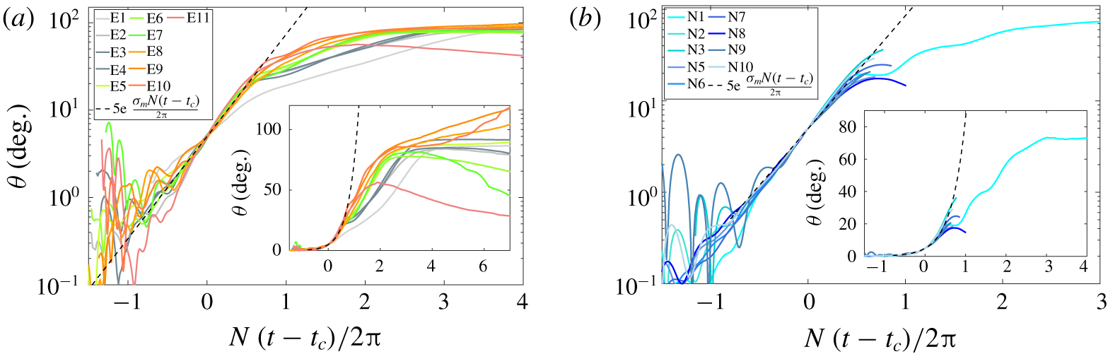
Temporal evolution of the orientation of the disk  $\unicode[STIX]{x1D703}$ for (a) experiments and (b) numerical simulations, along with the exponential growth using
 $\unicode[STIX]{x1D70E}_{m}$ (2.7 in a, 2.8 in b).

Then, the  $(0,0)$ equilibrium position becomes unstable and all trajectories follow a positive or negative branch (black dashed line, discussed in § 5.3) towards a new stability point
 $(\unicode[STIX]{x03C0}/2,0)$, with a clear change of stability towards edgewise settling. It should be noted that some trajectories do not reach this point before the end of settling, when the disk reaches its equilibrium depth before a complete change in orientation.
The final branch of the trajectories in figure 9(a) corresponds to phase 3, when the disk at its equilibrium depth rotates towards its non-zero equilibrium inclination angle in a quasi-static manner ( $\dot{\unicode[STIX]{x1D703}}/N\sim 0$).
5.3 Temporal evolution for the change of orientation
We focus now on the temporal evolution of the orientation of the disk for the same trajectories shown in figure 9. The results are presented in figure 10, with the same display for the experimental and numerical results. We set a common origin of time for an arbitrary orientation  $\unicode[STIX]{x1D703}=5^{\circ }$ corresponding to a time
 $t=t_{c}$. There is a good collapse of early dynamics for the orientation of all disks in (a) experiments and (b) numerical simulations. Furthermore, it is possible to model this early dynamics by an exponential growth, as expected for an instability mechanism, with
 $\unicode[STIX]{x1D703}(t)=5\exp [\unicode[STIX]{x1D70E}N(t-t_{c})/2\unicode[STIX]{x03C0}]$. Values for the growth rate
 $\unicode[STIX]{x1D70E}$ of each trajectory have been extracted and the mean value (
 $\unicode[STIX]{x1D70E}_{m}\simeq 2.7$) is similar for experiments and numerical simulations (2.7 and 2.8 respectively). No significant influence of the aspect ratio of the disk on
 $\unicode[STIX]{x1D70E}$ have been observed. At fixed value of
 $\unicode[STIX]{x1D712}$, small increases in
 $\unicode[STIX]{x1D70E}$ of 6 % and 10 % can also be observed when the viscosity increases by a factor 3 and 7 respectively (runs N
 $1$ to N
 $3$). The growth rate does not depend on the Archimedes, Froude, Reynolds or Richardson numbers either, and can be considered nearly constant in the range of values spanned.
It can be noted that the part of the trajectory corresponding to an exponential growth, is also reported in the phase diagrams in figure 9 by adding a dashed line for  $\unicode[STIX]{x1D703}(t)=5\exp [\unicode[STIX]{x1D70E}_{m}N(t-t_{c})/2/\unicode[STIX]{x03C0}]$.
5.4 Parameters influencing the observed threshold
The identification of the threshold for the broadside-on orientation to become unstable has shown some variations around a mean trend in terms of velocity, that can have several origins. The disks being manufactured from a long bar, there could be some imperfections in their design (uneven distribution of mass, asymmetry between the faces, etc.); fluid perturbations in the tank can also initiate some tilting of the disk, or there could be an influence of the initial release conditions of the disk.
Since the control of the initial conditions of release for the experimental disks is difficult, we have tested to let a numerical disk (run N $13$) settle from different initial angles
 $\unicode[STIX]{x1D703}_{i}$ (
 $0.6^{\circ },5^{\circ }$ and
 $11^{\circ }$), with no initial velocity. The disk changes its orientation at the same critical velocity for different initial angles, suggesting that the release conditions do not influence the identification of the threshold. Furthermore, especially for experimental cases, the long duration of the steady phase 1 makes it unlikely to influence the transition from broadside-on to edgewise settling. The influence of the confinement of the disk has also been tested numerically (see § A.2), without any noticeable effect on the values of the threshold for the vertical velocity. We now focus on the geometrical aspects.
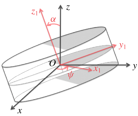
All experimental disks are slightly unbalanced, and this can affect the way this instability occurs and/or its corresponding threshold. A possible scenario could be that the imperfections in the mass distribution of the disk are initiating the change of stability in its orientation. A model for an unbalanced disk is presented in appendix C, with the overall geometry being unchanged but the density distribution being uneven, with one half of the disk having a density  $\unicode[STIX]{x1D70C}_{d}$ and the other half
 $\unicode[STIX]{x1D70C}_{d}(1+\unicode[STIX]{x1D716})$. Typical values for
 $\unicode[STIX]{x1D716}$ can be estimated from the observations made in § 4.4 and using (C 14), since it relates it to the angle
 $\unicode[STIX]{x1D6FC}$ of the disk with the horizontal when ending at its neutrally buoyant depth. For instance, with
 $\unicode[STIX]{x1D6FC}\simeq 15^{\circ }$ for run E
 $7$ or
 $35^{\circ }$ for run E
 $3$, the model predicts
 $\unicode[STIX]{x1D716}\simeq 7.3\times 10^{-5}$ or
 $1.2\times 10^{-4}$ respectively. Numerical simulations of an unbalanced disk, as modelled in appendix C with different values for
 $\unicode[STIX]{x1D716}$, are presented in figure 11. Other settling parameters are similar to run N
 $1$ except for
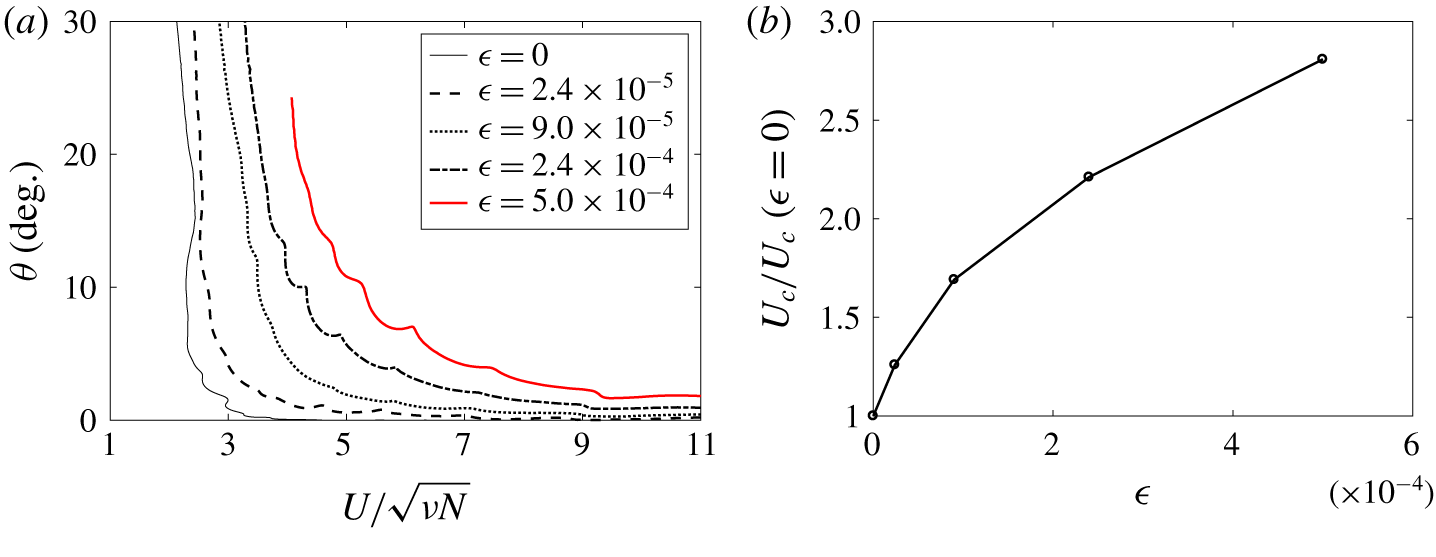
 $N=0.495~\text{rad}~\text{s}^{-1}$. The evolution of the orientation angle with the settling velocity is shown in figure 11(a). The case with
 $\unicode[STIX]{x1D716}=5\times 10^{-4}$ (red thick line) corresponds to an unbalanced disk that should sit vertical when reaching its neutral depth. One can observe that, with increasing values of
 $\unicode[STIX]{x1D716}$, the rotation of the disk is initiated at an earlier time in the settling process, hence at a higher velocity. In figure 11(b), the threshold for the normalized velocity is modified by
 $25\,\%$ with
 $\unicode[STIX]{x1D716}=2.4\times 10^{-5}$ and is more than double for
 $\unicode[STIX]{x1D716}=2.4\times 10^{-4}$. It should be noted that no modification of the temporal evolution of
 $\unicode[STIX]{x1D703}$ has been observed.
(a) Orientation angle  $\unicode[STIX]{x1D703}$ as a function of the vertical velocity
 $U$ normalized by
 $\sqrt{\unicode[STIX]{x1D708}N}$ for numerical runs studying the change of stability with unbalanced disks (runs similar to N
 $1$). (b) Evolution of the threshold velocity
 $U_{c}$ (at
 $\unicode[STIX]{x1D703}=5^{\circ }$) with
 $\unicode[STIX]{x1D716}$, compared to the case of a ‘perfect’ disk (
 $\unicode[STIX]{x1D716}=0$).

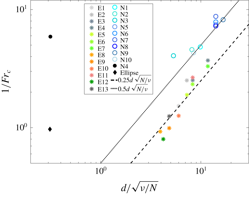
Threshold values shown as  $Fr_{c}$ as a function of
 $d/\sqrt{\unicode[STIX]{x1D708}/N}$ for all unstable cases. Two additional results are shown, run N
 $4$ is initially unstable, and ‘ellipsoid’ refers to parameters in Doostmohammadi & Ardekani (Reference Doostmohammadi and Ardekani2014).

These results are in good agreement with the experimental estimate for the threshold velocity that is almost twice larger than the value for the numerical disk, since the experimental disks are not perfectly made.
5.5 Stability domains for settling disks
Finally, from all these results, one can estimate the critical values for the parameters ( $Ar_{c}$,
 $Re_{c}$ and
 $Fr_{c}$) when the disks start to rotate by considering the values of the velocity of the disk
 $U_{c}$ and the density of the surrounding fluid
 $\unicode[STIX]{x1D70C}_{c}$, obtained at
 $t=t_{c}$ (
 $\unicode[STIX]{x1D703}_{c}=5^{\circ }$), which are close to the values at which the rotation starts. Since
 $Re/Fr$ is constant for each run, only
 $Ar_{c}=\sqrt{(\unicode[STIX]{x1D70C}_{d}/\unicode[STIX]{x1D70C}_{c}-1)gh}d/\unicode[STIX]{x1D708}$ and
 $Fr_{c}=U_{c}/Nd$ are relevant here.
When discussing this threshold in § 4.3, results led to the conclusion that  $U_{c}$ scales like
 $\sqrt{\unicode[STIX]{x1D708}N}$, although some dispersion of the threshold could be observed. The main reason is due to the quality of the experimental disks that are slightly unbalanced, as discussed in § 5.4, which could lead to a modification of
 $U_{c}$ (and hence in
 $Fr_{c}$) up to a factor
 $2$. Based on the scaling found for the velocity, the Froude number should follow
 $Fr_{c}\sim \sqrt{\unicode[STIX]{x1D708}/N}/d$, which is tested in figure 12. Here the experimental and numerical results have similar trends, which can be associated with
 $1/Fr_{c}\simeq 0.50(d/\sqrt{\unicode[STIX]{x1D708}/N})$ (dashed line) for the numerical simulations, and
 $1/Fr_{c}\simeq 0.25(d/\sqrt{\unicode[STIX]{x1D708}/N})$ (dotted line) for experimental values. These results are in reasonably good agreement with experiments and numerical simulations. They are also in agreement with the results in § 5.4 which showed that imperfect disks rotate earlier than perfect ones. Due to the dispersion of the extracted data, it must be noted that other models could match the data. For instance, experimental results could be better described by a power law of the type
 $1/Fr_{c}\simeq 0.16(d/\sqrt{\unicode[STIX]{x1D708}/N})^{1.25}$ and numerical results by
 $1/Fr_{c}\simeq 0.78(d/\sqrt{\unicode[STIX]{x1D708}/N})^{0.85}$. The physical implications for such threshold estimates remain unclear.
Nevertheless, these predictions provide a clear separation of domains in the  $(d/\sqrt{\unicode[STIX]{x1D708}/N},Fr)$ parameter space associated with a stable broadside-on or edgewise settling. We also include extra numerical results in figure 12 that confirm these stability domains. Run N
 $4$ in a very viscous stratified fluid initiated with
 $\unicode[STIX]{x1D703}_{i}=5^{\circ }$ revealed the broadside-on settling to be immediately unstable. The corresponding estimate for the threshold values reported in the figure is indeed located in the stable region for edgewise settling, i.e.
 $1/Fr>0.5(d/\sqrt{\unicode[STIX]{x1D708}/N})$. Similarly, we include results from Doostmohammadi & Ardekani (Reference Doostmohammadi and Ardekani2014) obtained for an ellipsoid at low Reynolds and Froude numbers released in a stratified fluid with
 $\unicode[STIX]{x1D703}_{i}=20^{\circ }$. The ellipsoid immediately rotates towards an edgewise settling, showing the stability of this orientation for an ellipsoid with
 ${\mathcal{R}}=1.1$,
 $\unicode[STIX]{x1D712}=2$,
 $Ar=15$,
 $Re=0.1$,
 $Fr=1.03$,
 $Pr=10^{3}$; indicated by a black diamond in figure 12.
Finally, we verified that the parameters of the threshold, expressed as  $Fr_{c}d/\sqrt{\unicode[STIX]{x1D708}/N}$, do not depend on
 $Ar_{c}$ (not shown). This suggests that there is no influence of the depth (or the local density
 $\unicode[STIX]{x1D70C}_{c}$) at which the transition occurs, and that the main physics of the change of stability is indeed in the critical Froude number.
6 Conclusion
We presented experimental and numerical results on the settling dynamics of a disk of finite thickness in a linearly stratified fluid. We characterized its dynamics at low and intermediate values of the Archimedes or Reynolds number ( $Ar$ and
 $Re$ in
 $0.1$ to
 $150$), and for Froude numbers in the range 0.01–4, showing the existence of two separate domains in the parameter space associated with stable broadside-on settling (high
 $Re/Ar$, high
 $Fr$) and edgewise settling (low
 $Re/Ar$, low
 $Fr$).
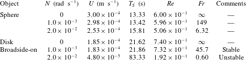
Settling parameters for an object of density  $\unicode[STIX]{x1D70C}_{p}=1040~\text{kg}~\text{m}^{-3}$, diameter
 $d=4~\text{mm}$ (and aspect ratio
 $\unicode[STIX]{x1D712}=3$ for the disk) in a fluid with
 $\unicode[STIX]{x1D70C}_{0}=1000~\text{kg}~\text{m}^{-3}$. The settling time is
 $T_{S}=d/U$.

We provided a parametric model for the stratified drag of the disk when settling broadside-on in a quasi-steady regime, inspired by a similar study based on buoyancy effects acting on the settling dynamics of a sphere in a linearly stratified fluid (Yick et al. Reference Yick, Torres, Peacock and Stocker2009). The relevant parameters for the modification of the drag are the Reynolds and Froude numbers and the aspect ratio of the disk. This parametric description can be of great interest to predicting the settling speed of anisotropic objects evolving in a stratified fluid. For instance, when considering plankton dynamics in the ocean, a discoid shape is a common feature for various oceanic species (Hillebrand et al. Reference Hillebrand, Dürselen, Kirschtel, Pollingher and Zohary1999; Clavano, Boss & Karp-Boss Reference Clavano, Boss and Karp-Boss2007) such as diatoms. Typical specifications for a microorganism are a radius of  $a\simeq 2~\text{mm}$, with aspect ratio
 $\unicode[STIX]{x1D712}=3$ and a nearly buoyant density
 $\unicode[STIX]{x1D70C}_{p}\simeq 1040~\text{kg}~\text{m}^{-3}$, while the stratification can vary from
 $N\simeq 10^{-3}~\text{rad}~\text{s}^{-1}$ in the deep ocean to peak values greater than
 $2.0\times 10^{-2}~\text{rad}~\text{s}^{-1}$ at sharp discontinuities (MacIntyre et al. Reference MacIntyre, Alldredge and Gotschalk1995). When modelling the settling speed of such microorganisms by a disk in a stratified environment, it is thus important to take into account both the effect of the geometry and of the stratification. The settling speed of a disk can be
 $2.5$ times smaller in a linearly stratified fluid than in the homogeneous case when the stratification is important (
 $N\simeq 10^{-2}$). It can be 2–5 times smaller than estimates made with the model of a sphere Yick et al. (Reference Yick, Torres, Peacock and Stocker2009) in the same environment, as summarized in table 2.
When discussing the change of stability for the orientation of the disk, we provided strong evidence of the instability mechanism, occurring at a threshold value for the vertical settling speed that can be discussed in terms of the Froude number  $Fr$, compared to intrinsic properties of the fluid and the disk. In the case of a ‘perfect’ disk, the threshold verifies
 $1/Fr_{c}\simeq 0.50(d/\sqrt{\unicode[STIX]{x1D708}/N})$, although some scattering observed in the data could lead to a different scaling. The growth rate of the instability has also been measured and is controlled by the Brunt–Väisälä frequency for both experiments and numerics, with a weak influence of the geometrical properties of the disks and the viscosity of the fluid. From our observations of the wake of the disk, we suggest that the mechanism driving this instability is associated with the displacement of the strongly localized low-pressure point at the centre of the back face of the disk when settling broadside-on, which induces a destabilizing torque on the disk in the horizontal direction. While reorientation of a disk in a homogeneous fluid at low Reynolds numbers is stabilized by a hydrodynamic torque (Fabre, Tchoufag & Magnaudet Reference Fabre, Tchoufag and Magnaudet2012), this effect seems to weaken in a stratified fluid when the vertical velocity of the disk decreases. This stabilizing effect can be overreached by the destabilizing stratified effect at sufficiently low values of
 $Re/Ar$ and
 $Fr$. This should be applicable to plankton dynamics, as discussed before, since low values of
 $Re/Ar$ and
 $Fr$ can be reached in the ocean (cf. comments in table 2).
There are numerous interesting perspectives for this study. The modelling of the stratification influence on the drag of an anisotropic bluff body, taking into account boundary layer effects, would provide a basis for the understanding of the competing effects of vorticity and buoyancy. The threshold estimates could be more precisely studied although it is computationally very expensive to resolve such stratified flows at high Prandtl numbers. Furthermore, a stability analysis for the change of preferential orientation for the disk is also required to understand the onset of instability, along with the temporal dynamics. A proper modelling of the torque on the disk (or on any object actually) in a stratified environment is still lacking. Finally, the instability of the orientation of the disk could be of great importance for the dynamics of a collection of anisotropic objects in a stratified medium, modifying the interactions and triggering instabilities in spatial distributions.
Acknowledgements
The authors would like to thank S. Belliot, S. Cazin, G. Ehses and M. Ogier for their help with the experimental set-up, and J. Albagnac for discussions on the equilibrium of a disk. Anonymous reviewers have also contributed to the quality of the manuscript. This work used the Extreme Science and Engineering Discovery Environment (XSEDE), which is supported by National Science Foundation grant numbers CTS180066 and CTS190055. M.J.M. is supported by ANR project F-PISE (ANR-13-PDOC-023). A.M.A. is supported by NSF CBET-16004423 and CBET-1705371.
Appendix A. Numerical validation
A.1 Grid resolution tests
In order to investigate the effect of grid resolution on the numerical modelling of the fluid perturbations (velocity and density) around the disk, we first consider two cases; a disk moving at a fixed speed with an imposed orientation ( $\unicode[STIX]{x1D703}=0$), and a sphere moving at a fixed speed as a reference case (already studied in Hanazaki et al. (Reference Hanazaki, Konishi and Okamura2009b, Reference Hanazaki, Nakamura and Yoshikawa2015)). This configuration allows us to compare the density and velocity in the jet for the same conditions (i.e. angle, velocity, etc) as a higher number of points around the disk is used. Additional computations have been done for numerical validation; the details of these additional computations are described in table 3. Since the objects have a fixed velocity, there is a precise value of the Froude and Reynolds numbers for each run,
 $Re=40$ (respectively 25) and
 $Fr=0.2$ (respectively 4) for the disks (respectively sphere).
Summary of the parameters for numerical simulations used as validations (labeled Nv $X$ with
 $X$ being a number).

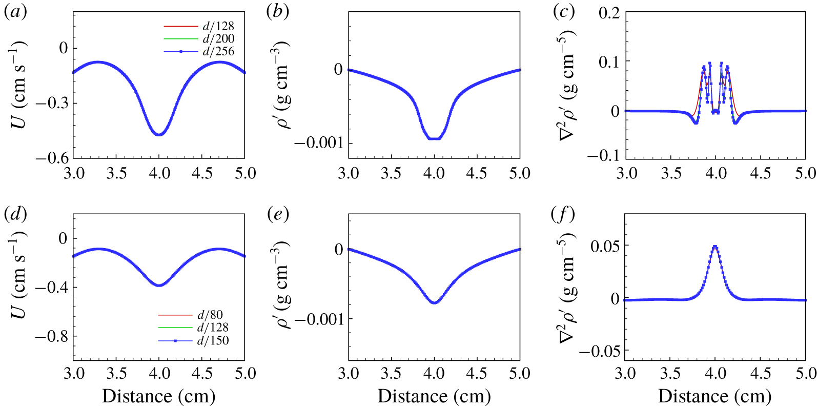
The results for the disk at two values of the Prandtl number are shown in figure 13, at time  $Nt/2\unicode[STIX]{x03C0}\simeq 0.8$ (
 $t=20~\text{s}$) after the start of motion. This time is chosen since it corresponds approximately to the time at which the instability in orientation occurs in the case of a freely settling disk (see run Nv
 $4$ below). Three different fields are displayed (velocity, density perturbation and its Laplacian), extracted along a horizontal line which is a half-radius away from the centre of the disk. As can be seen for all quantities, the grid resolution of
 $d/128$ is sufficient to get accurate values of velocity and density perturbation, although a resolution of
 $d/200$ is needed for the Laplacian of density to be properly resolved at
 $Pr=700$.
Distributions of (a,d) vertical velocity, (b,e) density perturbation and (c,f) Laplacian of density perturbation along a horizontal line within the settling plane crossing the centre of the disk, a half-radius away from the centre of the fixed disk ( $z=0.25d$). Both showcases are demonstrated at 20 s for run Nv
 $1$ (
 $Pr=700$) at the top and run Nv2 (
 $Pr=7$) at the bottom.

As time evolves, the jet in the wake of the disk gets thinner until it reaches a steady state. To verify this behaviour, we investigate the evolution of the jet radius, which is defined as the half-width at half-maximum of  $\unicode[STIX]{x1D6FB}^{2}\unicode[STIX]{x1D70C}^{\prime }$ along a horizontal line one radius away from the centre of the disk, similarly to Hanazaki et al. (Reference Hanazaki, Nakamura and Yoshikawa2015). We find the jet radius reaches a steady state at time of
 $Nt/2\unicode[STIX]{x03C0}=11$ for
 $Pr=700$, and
 $Nt/2\unicode[STIX]{x03C0}=3$ for
 $Pr=7$. while the sphere case is steady at
 $Nt/2\unicode[STIX]{x03C0}\simeq 3$, which is in agreement with the observations in Hanazaki et al. (Reference Hanazaki, Nakamura and Yoshikawa2015). Concerning the radius of the jet, the steady value reached
 $R/d=6\times 10^{-3}$ and
 $3\times 10^{-2}$ for the disk in Nv1 and Nv2 respectively; and
 $R/d=10^{-2}$ for the sphere, which is consistent with the prediction of
 $(Fr/2RePr)^{1/2}$ in Hanazaki et al. (Reference Hanazaki, Nakamura and Yoshikawa2015).
We now compare those results with the case of a freely settling disk (Nv4) in the next section, with the same physical parameters. In order to investigate the effect of grid resolution on the disk’s settling velocity, various grid resolutions are utilized in both horizontal and vertical directions (see figure 14a) for run Nv4 described in table 3. For the highest grid resolution, we use 256 grid points per disk diameter in the horizontal direction and 256 grid points per disk diameter in the vertical direction. This resolution is not sufficient to resolve fully the density perturbations developing in the jet at the rear of the disk when reaching a steady state, but it should remain sufficient for this scenario due to the temporal evolution of the instability which occurs before the jet gets very thin. When  $t\sim 20~\text{s}$ (
 $Nt/2\unicode[STIX]{x03C0}\sim 2$), the instability in terms of disk rotation occurs. The simulation results from 128 grid points per disk diameter in the horizontal and vertical directions are almost identical to the highest resolution. The orientation of the settling disk undergoes instability before the jet reaches steady state. Therefore, the jet thickness at the time of instability is wider than a steady jet and this resolution is sufficient to describe the instability. Overall, for horizontal and vertical resolutions of
 $d/128$, the relative error observed is
 $4\,\%$ for the density perturbation and
 $2\,\%$ for the vertical velocity (not shown here).
Orientation of the disk as a function of time in dimensional units (seconds). Numerical tests for (a) grid resolution for the settling parameters in run Nv4; (b) domain dependence for the settling parameters in run N8.

As a final remark, the central-difference scheme used for discretization of the diffusion term in our simulations is a second-order accurate scheme whereas the QUICK scheme used for discretization of the convection term has a third-order accuracy. Therefore, the overall accuracy remains as second order, which is consistent with our error test (not shown).
Comparison of numerical simulations Nv5, 6 and 7 with experimental runs E2, 5 and 7 respectively, in terms of velocity (a–c) and orientation angle of the disk (d–f) as a function of the normalized fluid density  $\unicode[STIX]{x1D70C}^{\star }$.

A.2 Domain dependence test
We investigate the effect of domain size on the problem for a run similar to N8 in the main part of the manuscript. The simulation result of angular velocity with time for a domain size of  $4d\times 4d\times 20d$ is compared to that for a domain size of
 $8d\times 8d\times 20d$ and
 $16d\times 16d\times 20d$ (see figure 14b), where
 $d$ is the disk’s radius. In addition, the simulations all provide a critical number
 $Ar_{c}$ of
 $152$. For all simulations, we use a width of
 $4d$. We should note that the purpose of the numerical simulation results is to understand the flow physics associated with phases 1 (quasi-steady state) and 2 (onset of the orientation instability). Here, the corresponding Reynolds number is approximately
 $26$ at the onset of the instability.
A.3 Direct comparison with experiments
We have simulated three different runs with physical parameters identical to experiments. We show direct comparison of these results with experiments. Runs Nv $5$,
 $6$ and
 $7$ (see table 3) correspond to experimental runs E
 $2$, E
 $5$ and E
 $7$ (see table 1). For each case plotted in figure 15, we follow the dynamics in terms of the non-dimensional velocity
 $U/U_{g}$ and the angle as a function of
 $\unicode[STIX]{x1D70C}^{\star }=1-(\unicode[STIX]{x1D70C}_{d}-\unicode[STIX]{x1D70C}(z))/(\unicode[STIX]{x1D70C}_{d}-\unicode[STIX]{x1D70C}_{0})$, with
 $U_{g}=\sqrt{(\unicode[STIX]{x1D70C}_{d}/\unicode[STIX]{x1D70C}_{0}-1)gh}$ a gravitational settling velocity. Each numerical run is initiated with the disk near the exact experimental release location, although not visible in the experiment (red lines start at values of
 $\unicode[STIX]{x1D70C}^{\star }\simeq 0.4$). Due to the long duration of these computations, only the early dynamics of the instability is reproduced (blue lines end before
 $\unicode[STIX]{x1D70C}^{\star }=1$).
Overall, the agreement between numerical simulations and experiments is good. The quasi-steady settling (phase 1) is well reproduced, and the initiation of the orientation instability occurs at very similar locations and with the same dynamics. These results confirm the validity of our approach, they are also in agreement with the results obtained for the estimate of the stratified drag coefficient in § 4.2, and the instability dynamics of the orientation of the disk in §§ 4.3 and 5.3.
Appendix B. Relation between the Archimedes and Reynolds numbers
Although it is common to discuss the dynamics of moving objects according to the Reynolds number, the Archimedes number is a more convenient non-dimensional parameter since it can be prescribed without knowing the velocity of the object. Figure 16(a) provides the evolution of  $Re$ and
 $Ar$ over the 3 phases of the overall dynamics of all experimental disks. Figure 16(b) validates the discussion in § 4.2 leading to (4.3) by testing the relation
 $2(Ar/Re)^{2}=C_{D}^{S}$ in phase 1.
(a) Value of  $Ar$ versus
 $Re$ for the overall dynamics of all experimental disks and (b)
 $2(Ar/Re)^{2}$ versus
 $C_{D}^{S}$ prescribed by (4.3) for all experimental disks. The dashed black line in (b) indicates the equality
 $2(Ar/Re)^{2}=C_{D}^{S}$.

Appendix C. Equilibrium orientation of an unbalanced disk in a stratified fluid
We consider the unbalanced disk shown in figure 17, with the prescribed orientation compared to the laboratory frame  $(O,x,y,z)$ given by the intrinsic and precession angles,
 $\unicode[STIX]{x1D713}$ and
 $\unicode[STIX]{x1D6FC}$, respectively, where the centre of the geometry is located at
 $O$. The axes of the frame associated with the disk,
 $(O,x_{1},y_{1},z_{1})$, are parallel to the principal axes of the inertia tensor. Indeed, the density of the disk
 $\unicode[STIX]{x1D70C}_{d}$ is constant for each half of the disk (
 $\unicode[STIX]{x1D70C}_{d}$ and
 $\unicode[STIX]{x1D70C}_{d}(1+\unicode[STIX]{x1D716})$), as indicated by the grey shading. We neglect the nutation of the disk due to the symmetry of the problem.
We define the following rotation matrices
 $$\begin{eqnarray}\unicode[STIX]{x1D63C}=\left(\begin{array}{@{}ccc@{}}\cos \unicode[STIX]{x1D713} & -\sin \unicode[STIX]{x1D713} & 0\\ \sin \unicode[STIX]{x1D713} & \cos \unicode[STIX]{x1D713} & 0\\ 0 & 0 & 1\end{array}\right)\quad \text{and}\quad \unicode[STIX]{x1D63D}=\left(\begin{array}{@{}ccc@{}}1 & 0 & 0\\ 0 & \cos \unicode[STIX]{x1D6FC} & -\sin \unicode[STIX]{x1D6FC}\\ 0 & \sin \unicode[STIX]{x1D6FC} & \cos \unicode[STIX]{x1D6FC}\end{array}\right),\end{eqnarray}$$
such that we can relate the two frames by
 $$\begin{eqnarray}\left(\begin{array}{@{}c@{}}x\\ y\\ z\end{array}\right)=\unicode[STIX]{x1D63D}\unicode[STIX]{x1D63C}\left(\begin{array}{@{}c@{}}x_{1}\\ y_{1}\\ z_{1}\end{array}\right).\end{eqnarray}$$
The disk is immersed in a linearly stratified fluid whose density is defined as
 $$\begin{eqnarray}\unicode[STIX]{x1D70C}(z)=\unicode[STIX]{x1D70C}_{0}\left(1-\frac{N^{2}z}{g}\right)=\unicode[STIX]{x1D70C}_{0}-\frac{N^{2}\unicode[STIX]{x1D70C}_{0}}{g}[z_{1}\cos \unicode[STIX]{x1D6FC}+\sin \unicode[STIX]{x1D6FC}(x_{1}\sin \unicode[STIX]{x1D713}+y_{1}\cos \unicode[STIX]{x1D713})],\end{eqnarray}$$
where (C 2) is used to express  $z$ in terms of the tilted coordinates.
Uneven disk made of two half-disks in the laboratory frame  $(x,y,z)$. The tilted frame
 $(x_{1},y_{1},z_{1})$ fixed to the disk is aligned with the principal axes of the inertia tensor. The densities of the white and grey halves are
 $\unicode[STIX]{x1D70C}_{d}$ and
 $\unicode[STIX]{x1D70C}_{d}(1+\unicode[STIX]{x1D716})$, respectively.

We study the torque resulting from the buoyancy force on the disk, which is given by
 $$\begin{eqnarray}\boldsymbol{{\mathcal{M}}}_{b}=\int \!\!\!\int \!\!\!\int _{{\mathcal{D}}}\boldsymbol{O}\boldsymbol{M}\wedge [\unicode[STIX]{x1D70C}_{d}(x,y,z)-\unicode[STIX]{x1D70C}(z)]\boldsymbol{g}\,\text{d}^{3}V.\end{eqnarray}$$
By considering the computation in the tilted frame and switching to cylindrical coordinates, we can rewrite (C 4) as
 $$\begin{eqnarray}\boldsymbol{{\mathcal{M}}}_{b}=\int _{-h/2}^{h/2}\int _{0}^{d/2}\!\!\!\int _{0}^{2\unicode[STIX]{x03C0}}\boldsymbol{O}\boldsymbol{M}_{1}\wedge [\unicode[STIX]{x1D70C}_{d}(\unicode[STIX]{x1D703}_{1})-\unicode[STIX]{x1D70C}(r_{1},\unicode[STIX]{x1D703}_{1},z_{1})]\boldsymbol{g}\,\text{r}_{1}\,\text{d}r_{1}\,\text{d}\unicode[STIX]{x1D703}_{1}\,\text{d}z_{1},\end{eqnarray}$$
where  $\boldsymbol{O}\boldsymbol{M}_{1}=r_{1}\boldsymbol{e}_{\boldsymbol{r}_{1}}+z_{1}\boldsymbol{e}_{\boldsymbol{z}_{1}}$ and
 $x_{1}=r_{1}\cos \unicode[STIX]{x1D703}_{1}$ and
 $y_{1}=r_{1}\sin \unicode[STIX]{x1D703}_{1}$. The density distribution of the disk
 $\unicode[STIX]{x1D70C}_{d}(\unicode[STIX]{x1D703}_{1})$ is defined as
 $$\begin{eqnarray}\unicode[STIX]{x1D70C}_{d}(\unicode[STIX]{x1D703})=\left\{\begin{array}{@{}ll@{}}\unicode[STIX]{x1D70C}_{d}(1+\unicode[STIX]{x1D716}) & \text{for }\unicode[STIX]{x1D703}\in [0,\unicode[STIX]{x03C0}]\\ \unicode[STIX]{x1D70C}_{d} & \text{for }\unicode[STIX]{x1D703}\in [\unicode[STIX]{x03C0},2\unicode[STIX]{x03C0}].\end{array}\right.\end{eqnarray}$$
The gravitational acceleration in the tilted frame is given as  $\boldsymbol{g}=-g(\cos \unicode[STIX]{x1D6FC}\,\boldsymbol{e}_{\boldsymbol{z}_{1}}+\sin \unicode[STIX]{x1D6FC}\sin \unicode[STIX]{x1D713}\,\boldsymbol{e}_{\boldsymbol{x}_{1}}+\sin \unicode[STIX]{x1D6FC}\cos \unicode[STIX]{x1D713}\,\boldsymbol{e}_{\boldsymbol{y}_{1}})$. This leads to the following expression for the vector product in (C 5)
 $$\begin{eqnarray}\boldsymbol{O}\boldsymbol{M}_{1}\wedge \boldsymbol{g}=g(r_{1}\cos \unicode[STIX]{x1D6FC}\,\boldsymbol{e}_{\unicode[STIX]{x1D73D}_{1}}+r_{1}\sin \unicode[STIX]{x1D6FC}(\sin \unicode[STIX]{x1D713}\sin \unicode[STIX]{x1D703}_{1}-\cos \unicode[STIX]{x1D713}\cos \unicode[STIX]{x1D703}_{1})\,\boldsymbol{e}_{\boldsymbol{z}_{1}}-z_{1}\sin \unicode[STIX]{x1D6FC}\,\boldsymbol{e}_{\boldsymbol{x}}).\end{eqnarray}$$
We now consider the integral in (C 5) which can be decomposed in the following manner,
 $$\begin{eqnarray}\displaystyle & & \displaystyle \hspace{-10.79993pt}\boldsymbol{{\mathcal{M}}}_{b}=\underbrace{\int _{-h/2}^{h/2}\!\int _{0}^{d/2}\!\!\!\int _{0}^{\unicode[STIX]{x03C0}}\!\!\left[\unicode[STIX]{x1D70C}_{d}(1+\unicode[STIX]{x1D716})-\unicode[STIX]{x1D70C}_{0}\right]\boldsymbol{O}\boldsymbol{M}_{1}\wedge \boldsymbol{g}\,r_{1}\,\text{d}r_{1}\,\text{d}\unicode[STIX]{x1D703}_{1}\,\text{d}z_{1}}_{I_{1}}+\cdots \nonumber\\ \displaystyle & & \displaystyle \hspace{-13.20007pt}\quad \underbrace{\int _{-h/2}^{h/2}\!\int _{0}^{d/2}\!\!\!\int _{\unicode[STIX]{x03C0}}^{2\unicode[STIX]{x03C0}}\!(\unicode[STIX]{x1D70C}_{d}-\unicode[STIX]{x1D70C}_{0})\boldsymbol{O}\boldsymbol{M}_{1}\wedge \boldsymbol{g}\,r_{1}\,\text{d}r_{1}\,\text{d}\unicode[STIX]{x1D703}_{1}\,\text{d}z_{1}}_{I_{2}}+\cdots \nonumber\\ \displaystyle & & \displaystyle \hspace{-13.20007pt}\quad \underbrace{\int _{-h/2}^{h/2}\!\int _{0}^{d/2}\!\!\!\int _{0}^{2\unicode[STIX]{x03C0}}\!\!\!\unicode[STIX]{x1D70C}_{0}N^{2}[z_{1}\cos \unicode[STIX]{x1D6FC}+r_{1}\sin \unicode[STIX]{x1D6FC}(\sin \unicode[STIX]{x1D713}\cos \unicode[STIX]{x1D703}_{1}\!+\!\cos \unicode[STIX]{x1D713}\sin \unicode[STIX]{x1D703}_{1})]\boldsymbol{O}\boldsymbol{M}_{1}\wedge \boldsymbol{g}\,r_{1}\,\text{d}r_{1}\,\text{d}\unicode[STIX]{x1D703}_{1}\,\text{d}z_{1}}_{I_{3}}\!.\nonumber\\ \displaystyle & & \displaystyle\end{eqnarray}$$
Integrals  $I_{1}$ and
 $I_{2}$ are complimentary and depend only on the distribution of density, whereas
 $I_{3}$ is only due to the stratification. The first two terms in (C 8) lead to
 $$\begin{eqnarray}I_{1}=-{\textstyle \frac{1}{12}}[\unicode[STIX]{x1D70C}_{d}(1+\unicode[STIX]{x1D716})-\unicode[STIX]{x1D70C}_{0}]ghd^{3}(\cos \unicode[STIX]{x1D6FC}\,\boldsymbol{e}_{\boldsymbol{ x}_{1}}-\sin \unicode[STIX]{x1D6FC}\sin \unicode[STIX]{x1D713}\boldsymbol{e}_{\boldsymbol{z}_{1}}),\end{eqnarray}$$
and
 $$\begin{eqnarray}I_{2}={\textstyle \frac{1}{12}}(\unicode[STIX]{x1D70C}_{d}-\unicode[STIX]{x1D70C}_{0})ghd^{3}(\cos \unicode[STIX]{x1D6FC}\,\boldsymbol{e}_{\boldsymbol{ x}_{1}}-\sin \unicode[STIX]{x1D6FC}\sin \unicode[STIX]{x1D713}\boldsymbol{e}_{\boldsymbol{z}_{1}}),\end{eqnarray}$$
such that
 $$\begin{eqnarray}I_{1}+I_{2}=-{\textstyle \frac{1}{12}}\unicode[STIX]{x1D70C}_{d}\unicode[STIX]{x1D716}ghd^{3}(\cos \unicode[STIX]{x1D6FC}\,\boldsymbol{e}_{\boldsymbol{ x}_{1}}-\sin \unicode[STIX]{x1D6FC}\sin \unicode[STIX]{x1D713}\boldsymbol{e}_{\boldsymbol{z}_{1}}).\end{eqnarray}$$
We now compute the term in the torque due to the presence of the stratified fluid. After some manipulations,  $I_{3}$ in (C 8) can be written as
 $$\begin{eqnarray}\displaystyle I_{3}=-\frac{\unicode[STIX]{x03C0}}{64}\unicode[STIX]{x1D70C}_{0}N^{2}hd^{4}\sin \unicode[STIX]{x1D6FC}\cos \unicode[STIX]{x1D6FC}\left(1+\frac{4}{3\unicode[STIX]{x1D712}^{2}}\right)\,\boldsymbol{e}_{\boldsymbol{x}}. & & \displaystyle\end{eqnarray}$$
Solutions  $(\unicode[STIX]{x1D716},\unicode[STIX]{x1D6FC})$ of (C 14) for a disk with
 $d=14~\text{mm}$,
 $\unicode[STIX]{x1D712}=8$ in a stratified fluid with
 $N=0.5~\text{rad}~\text{s}^{-1}$ and
 $\unicode[STIX]{x1D70C}_{0}=\unicode[STIX]{x1D70C}_{d}$ (
 $g=9.81~\text{m}^{2}~\text{s}^{-1}$).

In the end, the torque of the unbalanced disk in a stratified fluid is
 $$\begin{eqnarray}\boldsymbol{{\mathcal{M}}}_{b}=-\frac{1}{12}\unicode[STIX]{x1D70C}_{d}\unicode[STIX]{x1D716}ghd^{3}(\cos \unicode[STIX]{x1D6FC}\,\boldsymbol{e}_{\boldsymbol{ x}_{1}}-\sin \unicode[STIX]{x1D6FC}\sin \unicode[STIX]{x1D713}\boldsymbol{e}_{\boldsymbol{z}_{1}})-\frac{\unicode[STIX]{x03C0}}{128}\sin (2\unicode[STIX]{x1D6FC})\unicode[STIX]{x1D70C}_{0}N^{2}hd^{4}\left(1+\frac{4}{3\unicode[STIX]{x1D712}^{2}}\right)\,\boldsymbol{e}_{\boldsymbol{x}}.\end{eqnarray}$$
We can discuss the balance between the effect of the uneven density distribution and the stratification in (C 13) for the case  $\unicode[STIX]{x1D713}=0[\unicode[STIX]{x03C0}]$ without loss of generality. If
 $\unicode[STIX]{x1D713}\neq 0[\unicode[STIX]{x03C0}]$, the induced torque in the direction of
 $\boldsymbol{e}_{\boldsymbol{z}_{1}}$ leads to the rotation of the disk until
 $\unicode[STIX]{x1D713}=\unicode[STIX]{x03C0}$ (stable orientation with the heaviest part of the disk at the lowest depth).
If  $\unicode[STIX]{x1D713}=0[\unicode[STIX]{x03C0}]$, for a given stratification and geometry, the torque in (C 13) is in the direction of
 $\boldsymbol{e}_{\boldsymbol{x}}=\boldsymbol{e}_{\boldsymbol{x}_{1}}$, but can be positive or negative based on the signs of
 $\unicode[STIX]{x1D716}$ and
 $\unicode[STIX]{x1D6FC}$. It is possible to find an equilibrium tilted state, solution of
 $\boldsymbol{M}_{\boldsymbol{b}}=\mathbf{0}$, for an unbalanced disk if the distribution of mass satisfies
 $$\begin{eqnarray}\unicode[STIX]{x1D716}=-\frac{3\unicode[STIX]{x03C0}}{16}\frac{\unicode[STIX]{x1D70C}_{0}}{\unicode[STIX]{x1D70C}_{d}}\frac{N^{2}d}{g}\left(1+\frac{4}{3\unicode[STIX]{x1D712}^{2}}\right)\sin \unicode[STIX]{x1D6FC}.\end{eqnarray}$$
Based on the orientation in figure 17, the stable orientation indeed occurs for negative (respectively positive) values of  $\unicode[STIX]{x1D6FC}$ if
 $\unicode[STIX]{x1D716}$ is positive (respectively negative). Table 4 gives some examples for the pairs
 $(\unicode[STIX]{x1D716},\unicode[STIX]{x1D6FC})$ for a disk with
 $d=14~\text{mm}$,
 $\unicode[STIX]{x1D712}=8$ in a stratified fluid with
 $N=0.5~\text{rad}~\text{s}^{-1}$ and
 $\unicode[STIX]{x1D70C}_{0}=\unicode[STIX]{x1D70C}_{d}$. For this choice of parameters, comparable to the values studied in the manuscript, one can notice small values of
 $\unicode[STIX]{x1D716}$ are required for the disk to be nearly balanced. The disk used in our experiments have measured values of
 $\unicode[STIX]{x1D6FC}$ in the range
 $1^{\circ }$–
 $65^{\circ }$ (cf. figure 8 in § 4), corresponding to an uneven distribution of mass with
 $\unicode[STIX]{x1D716}\leqslant 10^{-4}$.