I. INTRODUCTION
Semiconducting crystalline nanowires (NWs) comprise a prospective class of materials for future electronic and nanoelectromechanical applications due to their superior electronic, mechanical, and piezoresistive properties.Reference Gao, Song, Liu and Wang1–Reference Parkinson, Lloyd-Hughes, Gao, Tan, Jagadish, Johnston and Herz8 Considering that fabrication of NW-based devices requires precise control over positioning and subsequent behavior of the NWs, it is evident that deeper understanding of NW–surface bilateral tribology mechanisms is crucial from both fundamental and practical points of view.
Several methods were used to investigate NW–substrate interaction.Reference Hsu and Chang9–Reference Zhu, Qin, Gu and Wang11 The most popular method consists in manipulation of NWs or nanotubes by atomic force microscope (AFM) tip, e.g., Falvo et al.Reference Falvo, Steele, Taylor and Superfine12 manipulated multiwall carbon nanotubes (CNTs) with AFM on a graphite substrate with simultaneous lateral force measurement. AFM provides a high precision of force control; however, AFM measurements are time-consuming due to the need of imaging after each manipulation step.
A simple approach, which utilizes the bent shape of a NW on a substrate to estimate the NW–substrate friction, was proposed by Bordag et al.Reference Bordag, Ribayrol, Conache, Fröberg, Gray, Samuelson, Montelius and Pettersson13 The profile of bent NW comes as a result of the interplay between elastic and friction forces. The modeled NW was assumed to form a circle with uniform distribution of elastic and friction forces along the NW. This method was applied for the study of static and kinetic friction and for determination of local strain in individual semiconductor NWs.Reference Conache, Gray, Ribayrol, Fröberg, Samuelson, Pettersson and Montelius14–Reference Conache, Ribayrol, Fröberg, Borgström, Samuelson, Montelius, Pettersson and Gray16 However, the model neglected the role of free NW ends and did not take into account the fact that the actual friction force vector may vary significantly along the NW’s length.
Strus et al.Reference Strus, Lahiji, Ares, Lopez, Raman and Reifenberger17 introduced a more sophisticated method, which also utilizes the shape of a CNT bent by AFM on substrate to compute static friction and flexural strain energy. Unfortunately, this method is highly sensitive to any inaccuracy in determination of the bent CNT or NW profile due to use of high-order derivatives. The eye-assisted skeletonization method of determining the bent CNT profile and unconsidered boundary conditions of zero force and momentum at the ends of the CNT may contribute significant error to the results.
In this article, we propose an alternative model of elastically bent NW lying on a flat substrate, which enables determination of friction forces between NW and the substrate. Appropriate skeletonization algorithm was elaborated utilizing specially selected polynomials for a curvature function, which conforms to the boundary conditions and significantly reduces possible errors in the friction force calculation. The method was tested on a ZnO NW bent into an arc during uniform dragging at its midpoint (B. Polyakov, L.M. Dorogin, R. Lõhmus, A. Lõhmus, and A.E. Romanov, unpublished data). An interpretation of the calculated static friction force is given and compared to the kinetic friction force for the same NW.
II. THEORETICAL BACKGROUND
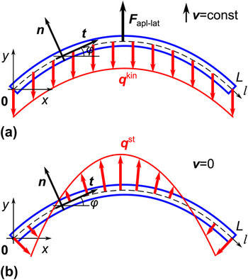
Let us consider a prismatic-shaped NW of length L, bent under external distributed forces [Figs. 1(a) and 1(b)]. The external forces may include both kinetic [Fig. 1(a)] and static [Fig. 1(b)] friction as well as driving force from the tip [Fig. 1(a)].
Schematics of a bent nanowire (NW) of length L affected by (a) kinetic friction force qkin and (b) distributed static friction force qst. Natural coordinates along the NWs axis l are vectors t and n. ϕ is the angle between the tangential vector t and the Ox axis.

We will designate the force and momentum of elastic stresses in a cross section of the NW as F and M, respectively. Their components can be written as an integral by the cross-section area S at any given point l of NW axisReference Timoshenko and Goodier18, Reference Landau and Lifshitz19:
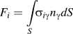
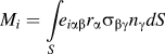
where σαβ is the stress tensor, nγ is the vector of normal to element of cross section area dS, rα is the radius vector from the point l, and eαβγ is the unit antisymmetric tensor. Both the elastic force F and the momentum M are considered as functions of the coordinate l along the NWs axis [Figs. 1(a) and 1(b)].
The full system of equilibrium equations for the NW consists of the equations for elastic force F and momentum MReference Landau and Lifshitz19:

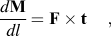
where f is the distributed external force acting on the NW per unit length and t is the tangent vector of the NW line. The force f may include the friction force between the NW and the substrate as well as the external concentrated forces.
The case of pure bending of prismatic shaped NW yields the following equation for momentumReference Landau and Lifshitz19:
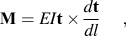
where E is the Young modulus of the NW and I is the moment of inertia of the cross section of the NW. Equation (3) describes the momentum of elastic forces inside a NW bent purely with the given curvature. Equation (3) can be projected to the Oz axis and written as
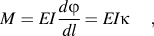
where ϕ(l) is the tangent angle function over the length of the NW and κ(l) = 1/R = dϕ/dl is the curvature function directly related to the radius of curvature R.
Zero elastic force and momentum at the free ends of the NW dictate the boundary conditionsReference Landau and Lifshitz19:


Equations (2a), (2b), and (3) together with the boundary conditions—Eqs. (5a) and (5b)—represent a full system of equations for determining the state of bent NW from known distributed external lateral force f.
III. KINETIC FRICTION
When a NW is being uniformly dragged at its midpoint and all parts of the NW have the same constant velocity, the equilibrium Eqs. (2a) and (2b) are still applicable. In this case, the profile of the deformed NW is determined by the balance of the external driving tip force, the kinetic friction between the NW, and the substrate and the intrinsic elastic forces of the NW. The distributed driving force Fapl−lat can be modeled via the delta function, and the kinetic friction qkin maintains a constant vector opposite to the direction of motion and Fapl−lat [Fig. 1(a)]:

The condition of zero total force yields  . The differential equation of “kinetic” equilibrium of the NW on the interval (0, L) directly follows from Eqs. (2) and (3):

where H(x) is the Heaviside step function. It is easy to see that the solution of Eq. (7) together with the initial condition ϕ′(0) = 0 fully complies with the boundary conditions Eq. (5a) and (5b).
IV. STATIC FRICTION
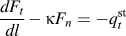
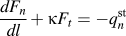
The equations of equilibrium for a purely bent NW affected by distributed static friction force qst(l) give [see Fig. 1(b) and, e.g., Ref. Reference Landau and Lifshitz19]:

where Ft and Fn,  , and
 are components of F and qst projected to the local coordinates (t, n), respectively.
We will neglect the tangential component of the friction  = 0, thus making the system of Eqs. (8a)–(8c) full and yielding:
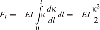
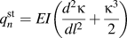
which solves the system together with the initial condition  . The absence of a tangential friction component does not lead to the vanishing of Ft which is then fully “driven” by the normal component Fn and necessary for strict NW equilibrium.
The complete set of boundary conditions—Eqs. (5a) and (5b)—at NW’s free ends dictate:

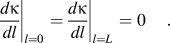
It is important to note that the assumption  was dictated by an intuitive consideration that the direction of qst should be nearly the same as the direction at which the NW tends to unbend. This “unbending” direction correspondingly lies close to normal to the NWs line. Formally one claims that the integral contribution of
 along the length of the NW is much smaller than that of
 .
V. RESULTS AND DISCUSSION
Consider a scanning electron microscope (SEM) or AFM image of a ZnO NW bent upon a substrate as a data source for static friction force analysis. We have developed an original method of skeletonization suitable for finding elastic and friction forces with use of Eq. (9). The method consist of several steps: (i) filtration of the source image and identification the backbone of the NW in Cartesian coordinates in the form of separate points; (ii) differential analysis of the backbone points to find the tangential angle curve; and (iii) interpolation of the tangential angle curve with polynomial function confined by the boundary conditions Eq. (5). As a result, we obtain a smooth polynomial function ϕ(l), which can be then utilized for the further  calculations according to Eq. (9b). A special polynomial function was chosen as a possible analytic form for Eq. (8). Let us now examine an application of this method in detail.
The source image snapshotted from a microscope usually contains some foreign objects (other NWs, nanoparticles, etc.). Everything except the NWs under investigation should be filtered out to avoid artifacts during the skeletonization. After filtration, the image is ready for the extraction of the backbone.
For locating the backbone, we used a polar-scanning method. We chose an origin point and observed the intersection of the polar beam with the NW. The intersection histogram commonly has an obvious peak which we assume to belong to the backbone curve. This method is best suited for curves bent in a circular manner, so that we can choose an origin point close to the circle’s center. However, any other method of backbone extraction can be used.
After the microscope image of the NW is skeletonized, a set of n discrete points (xi, yi) is obtained, representing the backbone. Differential analysis of the backbone is then needed to convert the Cartesian coordinates (xi, yi) to natural coordinates (li, ϕi), which are more suitable for the subsequent calculations. The discrete mesh for future ϕ(l) interpolation is produced with the following expressions:


where l 1 = 0.
Correct choice of the interpolation function is important, due to errors, which may arise during the identification and differentiation of the backbone curve. Regular polynomial interpolation would likely break the boundary conditions Eq. (5). The interpolation of ϕ(l) can be performed through the curvature κ(l) with the linear combination of the selected polynomial functions as follows:

where Ai are coefficients to be determined by the numerical interpolation. It is apparent that ϕ(l), defined according to Eq. (12), complies with the boundary conditions Eq. (5).
It should be noted that, the more asymmetric or wavy the NW curve looks, the higher the degree N that must be used. Higher N leads to increased precision in fitting the curves, but it also may introduce artifacts generated from the scatter of experimental points. Therefore, as low N as possible should be used, on condition of sufficient correspondence between the fitted and the original curves.
The friction profile can be now calculated with the Eq. (9b), using the constrains for κ(l) from Eq. (10). The expression for  contains the second derivative of the approximated κ(l) and therefore might contain significant error. As a consequence, the friction profile
 can vary significantly with N. As stated above, the usage of high N may introduce unnecessary features into the curve and therefore should be avoided.
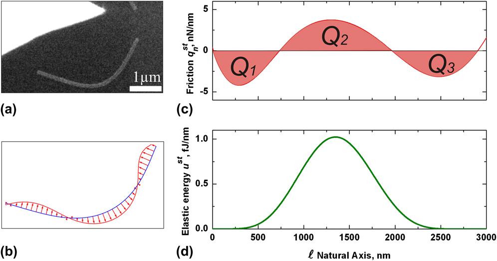
Let us now take, for instance, an experimental NW of ZnO resting on a silicon wafer substrate. In Fig. 2(a), an SEM image of a bent ZnO NW is presented. To prepare the NW in this bent state, it was pushed near its center perpendicular to the NW axis by an AFM tip inside the SEM (B. Polyakov, L.M. Dorogin, R. Lõhmus, A. Lõhmus, and A.E. Romanov, unpublished data). Over several microns of travel, the initially straight profile of the NW transformed into the characteristic arc shape. If the NW Young’s modulus of the NW is known, the distributed kinetic friction can be calculated according to Eq. (7). A distributed kinetic friction of q kin = 1.8 nN/nm was found for the given NW. The static friction force model can be applied after the removal of the force applied by the AFM tip.
Analysis of the intrinsic elastic and friction forces for a bent ZnO NW resting on a Si wafer substrate. (a) Scanning electron microscopy image of a bent NW (ZnO) lying on the substrate, (b) distribution diagram of static friction  along the NW, (c) diagram of static friction
 , and (d) diagram of strain energy u st. The approximation curve was obtained with an interpolation degree of N = 3.
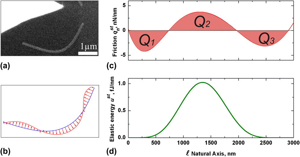
Prior to the calculation of  , a number of steps were performed as follows. The image was filtered manually. The backbone was extracted in the form of an array of Cartesian coordinates, and Eq. (11) was used to obtain the mesh of (li, ϕi) for further interpolation according to Eq. (12). Then the distributed friction force
 was calculated using Eq. (9b) [see Figs. 2(b) and 2(c)] taking into account
 for the hexagonal cross section of the NW,Reference Zhu, Chen, Gu, Warren and Osgood20 where D is the diameter of the NW. Polynomial functions of a degree of up to 7 were used, which corresponds to N = 3.
As was mentioned above, the shape and extreme values of  are sensitive to any errors in the interpolated NW profile and to the polynomial degree. Therefore, we must find reliable quantities able to characterize the NW–substrate system.
The friction profile  contains several ranges of length with different signs. We suggest using the following procedure to estimate the average friction forces acting on the different parts of the NW. When we integrate
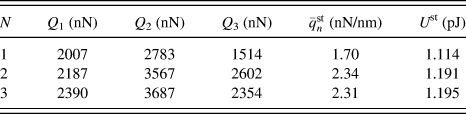
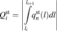 , the obtained quantity has the meaning of an effective force acting on the corresponding range. At least three regions, Q 1, Q 2, and Q 3, are necessary to stabilize the NW profile in its bent state [Fig. 2(c)]. Our calculations have shown that the Q i calculated using different N do not significantly change; however, a positive correlation of Q i with N is noticeable (see Table I). This behavior can be attributed to the fact that a curve of higher N is more wavy and therefore implies higher elastic distortion of the NW, which leads to higher friction. For the next step, a friction force averaged along the NW length
 is introduced. This along-NW-length-averaged friction force
 still remains nearly the same with different N, and it may be utilized to characterize the magnitude of the NW–substrate friction interaction.
The integrated friction forces Qi, averaged friction force and total elastic strain energy at different interpolation degrees N.
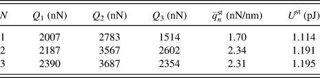
As it was stated above, the kinetic friction force is balanced with the force applied by the tip during the dragging of the NW over the substrate surface. We did not find any visual changes in the NW profile during the dragging and after the removal of the tip, hence elastic energy of deformed NW for static case should be preserved approximately the same with kinetic case. The static friction force should redistribute itself to maintain force balance with the elastic force, and value of averaged static friction should be comparable with one of kinetic friction. It should be noted here that the method for determination of the kinetic friction utilizes a more simple and faultless model than the static friction model (more details in Ref. Reference Polyakov, Dorogin, Vlassov, Kink, Lohmus, Romanov and Lohmus21, B. Polyakov, L.M. Dorogin, R. Lõhmus, A. Lõhmus, and A.E. Romanov, unpublished data). In other words, agreement between values of kinetic and averaged static friction will verify correctness or fault of static friction calculation method. The averaged static friction force  (1.7–2.34 nN/nm) has a value close to that of the kinetic friction q kin (1.8 nN/nm). This confirms appropriateness of our static friction calculation method.
An additional characteristic of the NW–substrate interaction is the elastic energy stored in the bent NW. The stronger the NW–substrate friction interaction, the higher the strain energy can be conserved in the elastically bent NW. The elastic energy per unit length u st and total elastic energy U stof bent NW can be calculated, respectively, asReference Landau and Lifshitz19:

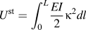
The profile of the distributed elastic energy u st is shown in Fig. 2(c). Values of the total elastic energy U st as a function of interpolation polynomial degree are given in Table I. The distributed elastic energy is proportional to the square of the NW curvature κ(l) and contains much smaller error compared to the friction force. Profiling of the distributed strain energy along the NW length and calculation of the total elastic energy may be important in piezotronics for engineering piezoresistive and piezoelectric NW-based devices.Reference Wang22
It is important to note that, while u st has only one extremum near the NW center, the distributed friction  experiences three extrema of different signs. This evidences a nonlocal character of the NW–substrate friction. Moreover, the model enables certain cases when
 has absolute maxima near the NW ends, rather than in the middle where the absolute maximum strain is located. Consequently, it is impossible to judge where the maximum friction is applied without detailed analysis in the framework of the presented distributed NW friction model.
We have demonstrated that our method produces reasonable values of the averaged friction force  and gives estimations of the distributed and total elastic energies U st. Thus, the method may provide important and useful information on NW–substrate force interactions.
VI. CONCLUSIONS
Computational models of kinetic and static friction for one-dimensional structures like NWs or nanotubes on a flat surface had been proposed. Kinetic friction between a substrate and NW being uniformly pushed at its midpoint by point force was found considering interplay between external forces and intrinsic elastic forces. Young’s modulus, cross section, and deformation profile of NW completely determine the magnitude of kinetic friction.
Model for calculation of distributed static friction force for NW bent and lying upon a flat surface was proposed. An appropriate NW backbone skeletonization algorithm was elaborated. The algorithm utilizes interpolation polynomials of special kind and enables explicit fulfillment of NW mechanic equilibrium.
Models were applied for calculation of distributed kinetic and static friction as well as elastic strain energy of ZnO NWs on a silicon wafer substrate pushed by an AFM tip and subsequently left to relax on the surface.
ACKNOWLEDGMENTS
B.P. was supported by the Estonian Science Foundation (Grant JD162). A.P. was supported by ESF Grant No. 2009/0202/1DP/1.1.1.2.0/09/APIA/VIAA/141. The work was also partly supported by Estonian Science Foundation Grant 8420, Estonian Nanotechnology Competence Centre (EU29996) and the ESF FANAS program “Nanoparma.”