



1. Introduction
The thermal resistance of a heat pipe may be smaller than that of a copper rod of the same diameter by a factor of one hundred or more (Faghri Reference Faghri1995). Consequently, they are ubiquitous in the thermal management of electronics (smart phones, laptops, server racks, etc.) and found in other applications such as the cooling of nuclear reactors (Zhao et al. Reference Zhao, Zhang, Zhang, Wang, Zhao, Li, Zhang and Gerada2022). Readers unfamiliar with heat pipes may consult an Annual Review of Fluid Mechanics article by Tien (Reference Tien1975) and Chapter 1 of the tome on heat pipes by Faghri (Reference Faghri1995).
Schematic of an AGHP.

Figure 1. Long description
Panel A: The schematic shows an adiabatic gravity-assisted heat pipe with three main sections: the evaporator section, the adiabatic section, and the finned condenser section. The evaporator section is positioned at the bottom, adjacent to a heat source. The adiabatic section connects the evaporator to the finned condenser section, which is located at the top. Panel B: A cross-sectional view of the finned condenser section shows the internal structure with fins. Panel C: A cross-sectional view of the evaporator section illustrates the presence of both liquid and vapor phases within the pipe.
A schematic of an axial-groove heat pipe (AGHP) with a circular cross-section and ‘open’ (as opposed to, say, screen-covered) grooves separated by protruding ‘lands’ is shown in figure 1. We define the angle
 $\phi \in { [-90^\circ , 90^\circ ]}$
as that between the axis of the AGHP and the gravity vector (of magnitude
 $g$
) and it is positive when its evaporator section is below its condenser one as shown. Axial-groove heat pipes are used in, e.g. the thermal management of electronics (Faghri Reference Faghri1995) and, since they are especially reliable on account of being monolithic (cf. heat pipes with screen-type wicks), space applications (Anand et al. Reference Anand, Vedamurthy, Chikkala, Kumar, Kumar and Gupta2008). We restrict our attention to straight AGHPs, but note that bends up to 180
 $^{\circ }$
are common in, e.g. the thermal management of laptop computers.
Heat is supplied to the evaporator section of an AGHP and rejected from the condenser one, which is often coupled to heat-dissipating fins, as shown in figure 1. In them, radial flows due to evaporation and condensation along menisci and due to changes in the cross-sectional area of the phases complicate transport phenomena. Between them is (usually) an adiabatic section. (An adiabatic section is not required in a heap pipe, but most possess one. For example, in the thermal management of a laptop computer, there is insufficient physical space and flow of air near the central processing unit (CPU) to accommodate a heat sink; therefore, commonly, a heat pipe with an adiabatic section is used to transfer the heat load to a strategically located condenser section thermally coupled to a heat sink) Invoking the common assumption of a ‘flat front’ between the evaporator and adiabatic sections and between the adiabatic and condenser ones, radial flows in the adiabatic section are exclusively due to changes in the cross-sectional areas of the phases (see e.g. Mills (Reference Mills1992) for a discussion of the flat-front assumption). Consequently, since this is the first study to account for axial variations in liquid–vapour interface (meniscus) curvature on the capillary limit, we focus it on the adiabatic section. (Effects of varying meniscus curvature in other contexts have been widely studied. Representatively, Khrustalev & Faghri (Reference Khrustalev and Faghri1995) provided the variation in the meniscus curvature based on resolving the pressure difference across the meniscus while assuming a constant cross-sectional area for both phases and Ranjan et al. (Reference Ranjan, Murthy, Garimella and Vadakkan2011) considered how it effects thin film evaporation and Marangoni convection in a wick) As shown by the insets in figure 1, in the adiabatic section, the meniscus curvature in the cross-plane is highest adjacent to the evaporator end of an AGHP and (generally) monotonically decreases to its value adjacent to its condenser end.
1.1. Capillary limit
The capillary limit of a heat pipe often provides the maximum rate at which heat may be transferred through it. Then, at larger heat loads, capillary forces are too weak to drive a sufficient mass flow rate of the working fluid at steady-state conditions. Consequently, an AGHP will dry out, i.e. intermittently possess a thermal resistance comparable to that for heat conduction through the axial-groove-containing tube housing the working fluid. Otherwise, in normal operation, there is liquid in the grooves along the entire length of the AGHP. The canonical expression for the capillary limit (see e.g. Faghri (Reference Faghri1995)) assumes that the meniscus has an infinite radius of curvature at the end of the condenser. It is given by
 \begin{equation} \Delta p_{\textit{cap,max}}^* = \Delta p_{\textit{l}}^* + \Delta p_{{v}}^* + \Delta p_{\textit{g}}^* + \Delta p_{\textit{e}}^* +\Delta p_{\textit{c}}^*, \end{equation}
where, throughout this paper, the
 $*$
superscript indicates a dimensional parameter, except for the always dimensional densities, viscosities, gravitational constant, latent heat of evaporation and surface tension. Here,
 $\Delta p_{\textit{cap,max}}^*$
is the maximum capillary pressure. We assume that the meniscus curvature in the (nominal) cross-plane is very large compared with that in the (nominal) orthogonal (streamwise) direction, as per the Young–Laplace equation, as given by Faghri (Reference Faghri1995),
 \begin{equation} \Delta p_{\textit{cap,max}}^*= \frac {\sigma }{R_{\textit{p,min}}^*}, \end{equation}
where
 $\sigma$
is the (liquid–vapour) surface tension and
 $R_{\textit{p,min}}^*$
is the minimum effective radius of curvature of a meniscus in a pore, i.e. a groove in an AGHP. From the geometry of the cross-section of an AGHP (see figure 2)
 \begin{equation} R_{\textit{p,min}}^* = \frac {R_{\textit{L}}^*\sin \left (\theta _{\textit{g}}/2\right )} {\sin \left (\pi /2 -\theta _{\textit{a}}+\theta _{\textit{g}}/2\right )}, \end{equation}
where
 $R_{\textit{L}}^*$
is the radius of a land,
 $\theta _{\textit{g}}$
is the azimuthal span of a groove and
 $\theta _{\textit{a}}$
is the advancing contact angle of the (wetting) liquid on the surface of the wick. On the right side of (1.1),
 $\Delta p_{\textit{l}}^*$
is the pressure drop due to liquid flow through the porous wick,
 $\Delta p_{{v}}^*$
is that due to vapour flow through the middle of the AGHP,
 $\Delta p_{\textit{g}}^*$
accounts for the component of the gravity force acting along the axis of the AGHP (this is normally negligible for the vapour phase; nonetheless, we retain the relevant term) and
 $\Delta p_{\textit{e}}^*$
and
 $\Delta p_{\textit{c}}^*$
are those associated with evaporation and condensation, respectively, along menisci, which can usually be neglected, an assumption we invoke. We further assume that a wet point, where pressures in both phases are the same, is at the end of the condenser. We express (1.1) as
 \begin{equation} \Delta p_{\textit{cap,max}}^* = \Delta p_{\textit{l,e}}^* +\Delta p_{\textit{v,e}}^* +\Delta p_{\textit{l,a}}^* +\Delta p_{\textit{v,a}}^* +\Delta p_{\textit{l,c}}^* +\Delta p_{\textit{v,c}}^*, \end{equation}
where e, a and c denote the evaporator, adiabatic and condenser sections of the AGHP, respectively, and gravity effects are implied to be within the terms stated rather than corresponding to their own term as in (1.1). This highlights the fact that, in most analyses of heat pipes, in addition to the flat-front assumption, the pressure gradients in the two phases are one-way coupled (i.e. vapour flow effects liquid flow but not vice versa as discussed in the following), if at all, a shortcoming we relax here for the adiabatic section.
Cross-sectional views of AGHP at arbitrary
 $z^*$
. (a) Full cross-section with domain bounded by dashed red curves and (b) domain. (Surfaces
 $\boldsymbol{A}$
-
 $\boldsymbol{M}$
are discussed in § 2.1 when boundary conditions are considered.)

We ignore axial conduction along the AGHP and the transfer of heat via sensible thermal energy changes. Then, the total rate of heat supplied to (and rejected by) the AGHP (
 $q_{\textit{t}}^*$
) is transferred through it by phase change and it is related to the (magnitude of the) mass flow rate of working fluid (in both phases) in the adiabatic section,
 $\dot {m}_{\textit{a}}^*$
, by
 \begin{equation} q_{\textit{t}}^*= \dot {m}_{\textit{a}}^* {h_{\textit{lv}}}, \end{equation}
where
 $h_{\textit{lv}}$
is the latent heat of evaporation of the working fluid (the magnitude of the mass flow rate in both phases is maximised in the adiabatic section). Engineers designing heat pipes must be able to compute
 $q_{\textit{t}}^*$
corresponding to the capillary limit, which we denote by
 $q_{\textit{cap}}^*$
. (the capillary limit problem is one of fluid mechanics – once it is known, the maximum rate of heat transfer follows from (1.5)) Note that other performance limits (sonic, boiling, entrainment, etc.; see Faghri (Reference Faghri1995)) may dictate the maximum load on a heat pipe and must be compared with it. The magnitude of the mass flow rate of working fluid in both phases increases from zero to its maximum value over the length of the evaporator section, remains there in the adiabatic section and decreases to zero over the length of the condenser section. Thus for any value of
 $z^*$
(the axial coordinate of the pipe)
 \begin{equation} q^*= \dot {m}^* {h_{\textit{lv}}}, \end{equation}
where
 $q^*$
is the net rate of heat input into the heat pipe (from the beginning of the evaporator section) and
 $\dot {m}^*$
is the magnitude of the local mass flow rate of both phases.
1.2. Literature review
Schneider & DeVos (Reference Schneider and DeVos1980) developed a model to calculate the capillary limit which accounted for the flows through the evaporator, adiabatic and condenser sections of an AGHP. Insofar as the vapour phase, since its velocity is (normally) much larger than that of the liquid one due to their density contrast (typically 3 orders of magnitude or more), a no-slip boundary condition was assumed at the meniscus. Consequently, the vapour-phase pressure drop was based on the friction factor for laminar flow through a circular tube. By implication, the vapour-phase problem is decoupled from the liquid-phase one. The liquid-phase pressure drop was found using the exact solution by DiCola (Reference DiCola1968) for the friction factor for flow through a rectangular channel with a uniform shear stress (taken from the solution to the vapour-phase problem and thus providing one-way coupling) at the meniscus and the no-slip boundary condition at liquid–solid interfaces. (It was also found by a less cumbersome approach that yielded good agreement with the aforementioned one by DiCola (Reference DiCola1968).) By implication, in the liquid-phase problem, the menisci are assumed to be flat, which is inconsistent with the solid–vapour interfaces being circular arcs in the vapour-phase problem. Other key assumptions in their model, which are common in the literature, are as follows. First, the cross-sectional areas of both phases are constant. Secondly, the flows were assumed quasi-steady and laminar, and the rate of heat transfer into and out of the evaporator and condenser sections, respectively, was uniform. Then, since laminar flow pressure gradients are proportional to mean velocity, the capillary limit is computed based on the mean velocity in the adiabatic section with the overall length of the AGHP equal to the sum of half the length of the evaporator section, the length of the adiabatic one and half the length of the condenser one.
Khrustalev & Faghri (Reference Khrustalev and Faghri1995) developed a model for the capillary limit of a circular (and rectangular) cross-section AGHP. Their model accounted for radial flow effects in the evaporator and condenser using friction factors and momentum-flux coefficients from the literature. The quasi-steady, highly viscous flow of liquid in the grooves was modelled using a friction factor expression developed by Schneider & DeVos (Reference Schneider and DeVos1980) to approximate the aforementioned solution by DiCola (Reference DiCola1968). Consequently, the component of the capillary limit attributable to the adiabatic section was essentially that in the Schneider & DeVos (Reference Schneider and DeVos1980) study.
Khrustalev & Faghri (Reference Khrustalev and Faghri1999) numerically resolved the liquid and vapour flows in a rectangular cross-section AGHP for the incompressible, quasi-steady problem for selected dimensionless parameters in the limiting case of unidirectional flows. They accounted for the contact angle between the liquid and vertical wall of the groove and thus captured the effects of meniscus curvature. Edge effects were neglected; consequently, as per lines of symmetry, the width of their domain extended from the middle of a land to the middle of the adjacent groove and was also bounded by the centre of the AGHP. When modelling the vapour phase, its velocity along menisci was assumed to be zero. After resolving the velocity field in the vapour phase, continuity of shear stress along the menisci enabled the resolution of that in the liquid phase. They showed that the shear stress exerted by the vapour phase on the liquid one is highly non-uniform, decreasing towards the centre of the meniscus, and that its importance decreases with increasing meniscus curvature. Their results were captured by providing friction factor–Reynolds number products for the vapour and liquid phases for representative values of the dimensionless independent variables. When using their friction factor–Reynolds number products to compute the capillary limit based upon the Khrustalev & Faghri (Reference Khrustalev and Faghri1995) study, predictions were within approximately 15 % of four experimental data points reported by Hopkins, Faghri & Khrustalev (Reference Hopkins, Faghri and Khrustalev1999).
Kim, Seo & Do (Reference Kim, Seo and Do2003) assumed the vapour flow was that through a circular tube to find the (uniform) shear stress exerted on the liquid phase in trapezoidal grooves. Moreover, they adapted the technique developed by Shah (Reference Shah1975) for duct flows to model open-channel flow in an arbitrary cross-section channel, where counter-flow is present on one interface, to compute the Poiseuille number for the liquid phase as a function of the contact angle. Anand et al. (Reference Anand, Vedamurthy, Chikkala, Kumar, Kumar and Gupta2008) used these results to model a (low temperature) aluminium AGHP with ethane as the working fluid for space applications.
The assumption of slowly varying meniscus curvature and thus cross-sectional area of the vapour and liquid phases is central to our analysis and, to our knowledge, new to the heat pipe literature. In a single-phase flow context, a similar assumption was first invoked by Blasius (Reference Blasius1910), who studied flows through (two-dimensional or axisymmetric) channels with slowly varying boundaries. A discussion on the limited use of it in internal flows since then is provided by Game, Hodes & Papageorgiou (Reference Game, Hodes and Papageorgiou2019). Generally, the slowly varying domain boundaries are prescribed and subjected to the no-slip condition. A notable exception is the study by Wild, Pedley & Riley (Reference Wild, Pedley and Riley1977), where elasticity conditions are imposed to model the (three-dimensional) flow of blood through elliptical cross-section channels. The Game et al. (Reference Game, Hodes and Papageorgiou2019) study considered liquid flow in the Cassie state through a superhydrophobic, parallel-plate geometry microchannel, where the menisci spanned ridges oriented parallel to the streamwise flow. The pressure drop across the microchannel was prescribed and the shape of the meniscus treated as an unknown. The leading-order streamwise problem and, to capture inertial effects, the leading-order transverse problem and first-order streamwise problem, were resolved. However, the meniscus was assumed to be shear free. (Earlier studies accounted for the gas phase trapped beneath menisci in the limit of fully developed flow; see e.g. Ng, Chu & Wang (Reference Ng, Chu and Wang2010), Game et al. (Reference Game, Hodes, Keaveny and Papageorgiou2017) and Crowdy (Reference Crowdy2017).)
Internal liquid flows in the Cassie state share many features with those through an AGHP. First, full resolution of the problem requires continuity of velocity and shear stress along menisci. Secondly, the locations of the menisci are unknowns. Thirdly, as in the case of an AGHP, heat may be used to drive liquid flow. However, for an internal flow in the Cassie state this would be done via exploiting thermocapillary stress along menisci (see e.g. Baier, Steffes & Hardt Reference Baier, Steffes and Hardt2010; Crowdy, Mayer & Hodes Reference Crowdy, Mayer and Hodes2023), a secondary effect in an AGHP. A key distinction, however, is that in an AGHP the liquid resides in the grooves and the vapour in the core and vice versa in the flow of liquid in the Cassie state. In addition, the gas phase recirculates with zero net flow rate in an internal flow in the Cassie state but, on average, it flows counter to the liquid in an AGHP.
In closing our discussion on liquid flows through tubes, etc. in the Cassie state, we note that numerous permutations of them have been resolved. Usually a Cartesian or polar coordinate system suffices insofar as imposition of boundary conditions at constant values of a coordinate – see e.g. Lauga & Stone (Reference Lauga and Stone2003), Zimmermann, Schönecker & Crowdy (Reference Zimmermann, Schönecker and Crowdy2025). However, as in the present work, this entails a degree of approximation as the pressure difference across and therefore radius of curvature of menisci is not constant. Such problems have been resolved by, e.g. a boundary perturbation by Kirk, Hodes & Papageorgiou (Reference Kirk, Hodes and Papageorgiou2017), conformal maps, etc. by Crowdy (Reference Crowdy2016) and the use of bipolar coordinates by Yariv & Kirk (Reference Yariv and Kirk2021).
1.3. Current work
The present model provides a means to compute the component of the capillary limit attributable to the adiabatic section of an AGHP. It is compatible with existing models for the evaporator and condenser sections as per § 4 and distinct from previous models for the following reasons. First, we do not assume that the vapour velocity along menisci is zero, which, in and of itself, causes a non-uniform shear stress along menisci. Rather we solve the fully coupled problem, where velocities and shear stresses are matched at menisci. Secondly, the radius of curvature along menisci is treated as unknown and its streamwise (or axial) variation is resolved. Finally, our formulation is based on the asymptotics which follow from the assumption of slowly varying meniscus curvature, which implies the following. First, our results for the limiting case, i.e. leading-order problem, when the radius of the meniscus is constant (not slowly varying) and equal to that of the lands, are semi-analytical. Secondly, the order of the asymptotic error from the slowly varying assumption is provided. Thirdly, our formulation is readily extended to account for inertial effects (due to varying cross-sectional areas of the phases on account of the meniscus curvature gradient), which are included in § 2, but drop out of the leading-order streamwise problem we solve. We also outline a boundary perturbation (and quantify the error associated with it) to account for the difference between the radii of curvature of the lands and menisci rather than resorting to a numerical solution. (This implies the variation in meniscus curvature is small, in addition to slow, assumptions combined in the study by Van Dyke (Reference Van Dyke1983) on laminar flow through meandering channels.) We do not provide Poiseuille numbers corresponding to our results as, because the phases are fully coupled, they would depend upon an unwieldy number of dimensionless variables.
2. Formulation of three-dimensional problem
2.1. Domain and governing equations
A cross-sectional view of an AGHP (representatively made out of copper) is shown in figure 2(a). Note that a criterion on the transverse Bond numbers (see (2.40)) required to assume that all menisci have the same radius of curvature (at a given axial location in the adiabatic section), as delineated in figure 2, is provided below. Looking ahead, once we justify the slowly varying meniscus curvature assumption in § 2.3, for our purposes, we need only resolve a series of two-dimensional problems and some related integrals across the adiabatic section to compute the capillary limit. In the
 $ (r^*,\theta ,z^* )$
cylindrical coordinate system shown,
 $z^*$
is the streamwise coordinate, directed from the evaporator to the condenser, and
 $r^*$
and
 $\theta$
are the transverse ones, with positive
 $\theta$
anti-clockwise. The adiabatic section begins at
 $z^* = 0$
, where the evaporator one ends. There are
 $N_{\textit{g}}$
grooves (and lands); consequently, their (azimuthal) pitch is
 \begin{equation} \theta _{\textit{p}} = \frac {2\pi }{N_{\textit{g}}}. \end{equation}
The radius of the grooves is denoted by
 $R_{\textit{g}}^*$
. Observe that the vapour phase is continuous, but there are
 $N$
discrete liquid regions in the full problem. However, our domain includes only half of one of them; therefore, it is bounded by the dashed, red curves and has an azimuthal span of
 $\pi /N_{\textit{g}}$
. It extends over the length of the adiabatic section from
 $z^* = 0$
to
 $z^* = L_{\textit{a}}^*$
, where the condenser section begins. An enlarged view of its cross-section is shown in figure 2(b). The boundaries (
 $\boldsymbol{F}$
,
 $\boldsymbol{G}$
and
 $\boldsymbol{H}$
) at
 $\theta = 0$
,
 $\theta _{\textit{p}}/2$
become flow symmetry boundaries once the effect of the in-plane components of gravity are neglected, which we justify in § 2.3.
We assume constant density (
 $\rho$
) and viscosity (
 $\mu$
) and laminar, incompressible flow in the liquid and vapour phases. (The maximum Reynolds and Mach numbers in both phases for the range of operating conditions considered are provided in § 7 and are sufficiently low.) Then, for the steady-state conditions of interest, the continuity and Navier–Stokes equations are
 \begin{align} \boldsymbol{\nabla} ^* \boldsymbol{\cdot }\boldsymbol{v}_i^* &= 0, \end{align}
 \begin{align} \rho _i \boldsymbol{v}_i^* \boldsymbol{\cdot }\boldsymbol{\nabla} ^* \boldsymbol{v}_i^*&= - \boldsymbol{\nabla} ^* p_i^* + \mu _i \boldsymbol{\nabla} ^{*^2} \boldsymbol{v}_i^*+\rho _i \boldsymbol{g}, \end{align}
respectively, where the subscript
 $i$
denotes the liquid (
 $\textit{l}$
) or vapour (
 ${v}$
) phase and
 $\boldsymbol{g}$
is the gravity vector. Also,
 $\boldsymbol{v}^*_i = v_r^*\boldsymbol{\delta }_{r^*} +v_{\theta }^*\boldsymbol{\delta }_{\theta }+ v_z^*\boldsymbol{\delta }_{z^*}$
is the velocity vector, where
 $\boldsymbol{\delta }_{i}$
denotes a unit vector in the
 $i$
direction, and
 $p_i^*$
is pressure. The gravity vector is
 \begin{equation} \boldsymbol{g} = -g \cos (\phi) \sin \left (\theta \right )\boldsymbol{\delta }_{r^*} -g \cos (\phi) \cos \left (\theta \right )\boldsymbol{\delta }_{\theta } - g \sin (\phi) \boldsymbol{\delta }_{z^*}, \end{equation}
where
 $g$
is the standard acceleration of gravity, 9.81 m s
 $^{-2}$
. The ‘inventory’ or ‘fill ratio’ of working fluid in the heat pipe is assumed to be such that the triple-contact lines are pinned at the top of the grooves.
2.2. Boundary conditions
We define the location of the meniscus by the unknown vector function
 \begin{equation} \boldsymbol{L} = R_{{v}}^*\left (\theta ,z^*\right ) \boldsymbol{\delta }_{r^*} + z^*\boldsymbol{\delta }_{z^*}. \end{equation}
Then, the surfaces bounding the domain labelled in figure 2(b) are defined in table 1 (surface M would appear in a boundary perturbation with the meniscus Taylor expanded onto
 $r^* = R_{\textit{L}}^*$
).
Domain boundaries.

Table 1. Long description
The table has 13 rows and 5 columns. The columns are labeled Surface, Phase(s), z∗, r∗, and theta. The rows are labeled with letters A to M. Each row provides specific values and conditions for the location of the meniscus and surfaces bounding the domain. Row 1: Surface A, Phase(s) Vapour, z∗ 0, r∗ 0 < r∗ < R∗_v for 0 < theta < theta_g/2, 0 < r∗ < R∗_L for theta_g/2 < theta < theta_p/2, theta 0 < theta < theta_p/2. Row 2: Surface B, Phase(s) Liquid, z∗ 0, r∗ R∗_v < r∗ < R∗_g, theta 0 < theta < theta_g/2. Row 3: Surface C, Phase(s) Vapour, z∗ L∗_a, r∗ 0 < r∗ < R∗_v for 0 < theta < theta_g/2, 0 < r∗ < R∗_L for theta_g/2 < theta < theta_p/2, theta 0 < theta < theta_p/2. Row 4: Surface D, Phase(s) Liquid, z∗ L∗_a, r∗ R∗_v < r∗ < R∗_g, theta 0 < theta < theta_g/2. Row 5: Surface E, Phase(s) Vapour, z∗ 0 < z∗ < L∗_a, r∗ 0, theta Not applicable. Row 6: Surface F, Phase(s) Vapour, z∗ 0 < z∗ < L∗_a, r∗ 0 < r∗ < R∗_v, theta 0. Row 7: Surface G, Phase(s) Vapour, z∗ 0 < z∗ < L∗_a, r∗ 0 < r∗ < R∗_L, theta theta_p/2. Row 8: Surface H, Phase(s) Liquid, z∗ 0 < z∗ < L∗_a, r∗ R∗_v < r∗ < R∗_g, theta 0. Row 9: Surface I, Phase(s) Solid-liquid, z∗ 0 < z∗ < L∗_a, r∗ R∗_L < r∗ < R∗_g, theta theta_g/2. Row 10: Surface J, Phase(s) Solid-vapor, z∗ 0 < z∗ < L∗_a, r∗ R∗_L, theta theta_p/2 < theta < theta_g/2. Row 11: Surface K, Phase(s) Solid-liquid, z∗ 0 < z∗ < L∗_a, r∗ R∗_g, theta 0 < theta < theta_g/2. Row 12: Surface L, Phase(s) Meniscus, z∗ 0 < z∗ < L∗_a, r∗ R∗_v, theta 0 < theta < theta_g/2. Row 13: Surface M, Phase(s) Meniscus, z∗ 0 < z∗ < L∗_a, r∗ R∗_L, theta 0 < theta < theta_g/2.
We define the pressures in the vapour and liquid phases at
 $z^*=0$
and
 $z^* = L_{\textit{a}}^*$
as per
 \begin{align} p_{{v}}^* &= p_{\textit{v,e}}^*\,\mathrm{on}\,\boldsymbol{A}, \end{align}
 \begin{align} p_{\textit{l}}^* &= p_{\textit{l,e}}^*\,\mathrm{on}\,\boldsymbol{B}, \end{align}
 \begin{align} p_{{v}}^* &= p_{\textit{v,c}}^*\,\mathrm{on}\,\boldsymbol{C}, \end{align}
 \begin{align} p_{\textit{l}}^* &= p_{\textit{l,c}}^*\,\mathrm{on}\,\boldsymbol{D}, \end{align}
where the subscripts e and c indicate that surfaces
 $\boldsymbol{A}$
and
 $\boldsymbol{B}$
and surfaces
 $\boldsymbol{C}$
and
 $\boldsymbol{D}$
are at the ends of the adiabatic section adjacent to the evaporator and condenser, respectively. The (streamwise) mass flow rates of working fluid in the liquid and vapour phases in the adiabatic section are equal in magnitude and thus satisfy
 \begin{equation} \int _{0}^{ \theta _{\textit{g}}/2 } \int _{0}^{R_{{v}}^*}v_{z^*,{v}}^*r^*\mathrm{d}r^*\mathrm{d}\theta + \int _{\theta _{\textit{g}}/2}^{{\theta _{\textit{p}}}/2} \int _{0}^{R_{\textit{L}}^*}v_{z^*,{v}}^*r^*\mathrm{d}r^*\mathrm{d}\theta = -\frac {1}{\tilde {\rho }}\int _{0}^{\theta _{\textit{g}}/2}\int _{R_{{v}}^*}^{R_{\textit{g}}^*}v_{z^*,\textit{l}}^*r^*\mathrm{d}r^*\mathrm{d}\theta , \end{equation}
where
 $\tilde {\rho } = \rho _{{v}}/\rho _{\textit{l}}$
.
Turning to the boundary conditions, the radial symmetry condition applies through line
 $\boldsymbol{E}$
passing through the centre of the domain at
 $r^* = 0$
as per
 \begin{align} v_{r^*,{v},r^*}^* &= v_{\theta ,{v},r^*}^* = v_{z*,{v},r^*}^*= 0\,\mathrm{on}\,\boldsymbol{E}, \end{align}
 \begin{align} p_{{v},r^*}^*& = 0\,\mathrm{on}\,\boldsymbol{E}, \end{align}
where the last variable in a subscript denotes a partial derivative. Mirror symmetry boundary conditions apply along surfaces
 $\boldsymbol{F}$
,
 $\boldsymbol{G}$
and
 $\boldsymbol{H}$
as per
 \begin{align} v_{r^*,{v},\theta }^*&=0,v_{\theta ,{v}}^*=0,v_{z^*,{v},\theta } ^*= p_{{v},\theta }^* = 0\,\mathrm{on}\,\boldsymbol{F}, \end{align}
 \begin{align} v_{r^*,{v},\theta }^*&=0,v_{\theta ,{v}}^*= 0,v_{z^*,{v},\theta }^*=0\,\mathrm{on}\,\boldsymbol{G}, \end{align}
 \begin{align} v_{r^*,\textit{l},\theta }^*&=0,v_{\theta ,\textit{l}}^*= 0,v_{z^*,\textit{l},\theta }^*=0\,\mathrm{on}\,\boldsymbol{H}. \end{align}
(This is justified below by showing that gravity effects transverse to the flow are small.) The no-slip and impermeability boundary conditions apply along both solid–liquid interfaces and the solid–vapour one as per
 \begin{align} \boldsymbol{v}_{\textit{l}}^* &= 0\,\mathrm{on}\,\boldsymbol{I}, \end{align}
 \begin{align} \boldsymbol{v}_{{v}}^* &=0\,\mathrm{on}\,\boldsymbol{J}, \end{align}
 \begin{align} \boldsymbol{v}_{\textit{l}}^* &=0\,\mathrm{on}\,\boldsymbol{K}. \end{align}
Turning to the boundary conditions along the meniscus, we define two (linearly independent) unit tangent vectors along it,
 $\hat {\boldsymbol{t}}_{\perp }$
in a (nominally) transverse (constant
 $z^*$
) direction and
 $\hat {\boldsymbol{t}}_{\textit{s}}$
in a (nominally) streamwise (constant
 $\theta$
) direction, and the corresponding unit normal pointing into the vapour phase (
 $\hat {\boldsymbol{n}}$
). They are
 \begin{align} \hat {\boldsymbol{t}}_{\perp } = \frac {R_{{v},\theta }^*/R_{{v}}^* \boldsymbol{\delta }_{r^*}+\boldsymbol{\delta }_{\theta }} {\sqrt {1+\big (R_{{v},\theta }^*/R_{{v}}^*\big )^2}} ;\, \hat {\boldsymbol{t}}_{\textit{s}} = \frac {R_{{v},z^*}^*\boldsymbol{\delta }_{r^*}+ \boldsymbol{\delta }_{z^*}} { \sqrt { 1+R_{{v},z^*}^{*^2} } };\, \hat {\boldsymbol{n}} = \frac { -\boldsymbol{\delta }_{r^*} + R_{{v},\theta }^*/R_{{v}}^*\boldsymbol{\delta }_{\theta } +R_{{v},z^*}^*\boldsymbol{\delta }_{z^*} } {\sqrt { 1+ \big (R_{{v},\theta }^{*}/R_{{v}}^*\big ) ^2 +R_{{v},z^*}^{*^2} } }. \end{align}
Relatedly, twice the mean curvature of the meniscus, which we denote by
 $\kappa ^*$
, equals
 $-\boldsymbol{\nabla }\boldsymbol{\cdot }\hat {\boldsymbol{n}}$
.
Along the meniscus, the impermeability condition as well as the continuity of velocities and the continuity of tangential stresses and normal stress apply as per
 \begin{align} \boldsymbol{v}_{{v}}^*\boldsymbol{\cdot }\hat {\boldsymbol{n}} &= 0\,\mathrm{on}\,\boldsymbol{L}, \end{align}
 \begin{align} \boldsymbol{v}_{{v}}^*&= \boldsymbol{v}_{\textit{l}}^*\,\mathrm{on}\,\boldsymbol{L}, \end{align}
 \begin{align} \left (p_{{v}}^*-p_{\textit{l}}^*\right )\hat {\boldsymbol{n}} + \hat {\boldsymbol{n}}\boldsymbol{\cdot }\left (\boldsymbol{\tau }_{\textit{l}}^* -\boldsymbol{\tau }_{{v}}^*\right ) &= \kappa ^*\,\sigma \,\hat {\boldsymbol{n}} \,\mathrm{on}\,\boldsymbol{L}, \end{align}
respectively (Landau & Lifshitz Reference Landau and Lifshitz1988). Here,
 $\boldsymbol{\tau }_i^*$
is the viscous stress tensor as per
 \begin{equation} \boldsymbol{\tau }_i^*= \mu _i \left [\boldsymbol{\nabla} ^*\boldsymbol{v}_i^*+ \left (\boldsymbol{\nabla} ^*\boldsymbol{v}_i^*\right )^{\mathrm{T}}\right ], \end{equation}
and
 $\sigma$
is surface tension. In expanded form, the impermeability condition becomes
 \begin{equation} -v_{r^*,{v}}^* + \frac {R_{{v},\theta }^*}{R_{{v}}^*}v_{\theta ,{v}}^* +R_{{v},z^*}^* v_{z^*,{v}}^* = 0\,\mathrm{on}\,\boldsymbol{L}, \end{equation}
and the continuity of velocities manifests itself as
 \begin{equation} v_{r^*,{v}}^* = v_{r^*,\textit{l}}^*;\,v_{\theta ,{v}}^*= v_{\theta ,\textit{l}}^*;\,v_{z^*,{v}}^*=v_{z^*,\textit{l}}^* \,\mathrm{on}\,\boldsymbol{L}. \end{equation}
Dotting the unit tangent vectors into the stress balance along the meniscus (2.22), the tangential stress balances in the transverse and streamwise directions become
 \begin{equation} \hat {\boldsymbol{t}}_{\perp }\boldsymbol{\cdot }\hat {\boldsymbol{n}}\boldsymbol{\cdot }\left (\boldsymbol{\tau }_{\textit{l}}^* -\boldsymbol{\tau }_{{v}}^*\right )=0,\, \hat {\boldsymbol{t}}_{\textit{s}}\boldsymbol{\cdot }\hat {\boldsymbol{n}}\boldsymbol{\cdot }\left (\boldsymbol{\tau }_{\textit{l}}^* -\boldsymbol{\tau }_{{v}}^*\right )=0\,\mathrm{on}\,\boldsymbol{L} , \end{equation}
respectively. Also, dotting the unit normal vector into the stress balance along the meniscus (2.22), the normal stress balance becomes
 \begin{equation} p_{{v}}^*-p_{\textit{l}}^* +\hat {\boldsymbol{n}}\boldsymbol{\cdot }\hat {\boldsymbol{n}}\boldsymbol{\cdot }\left (\boldsymbol{\tau }_{\textit{l}}^* -\boldsymbol{\tau }_{{v}}^*\right ) = \kappa ^*\,\sigma \,\mathrm{on}\,\boldsymbol{L}. \end{equation}
2.3. Slowly varying assumption and non-dimensionalisation
Normally, in an AGHP, the arc lengths spanning the bases of the grooves, menisci and tops of the lands are comparable, and of the same scale as the depth of the grooves (
 $R_{\textit{g}}^*-R_{\textit{L}}^*$
). Consequently, a key length scale is the groove pitch,
 \begin{equation} P^* = \theta _{\textit{p}}R_{\textit{L}}^*. \end{equation}
Also, the pitch of the grooves is normally small compared with the length of the adiabatic section, as is the radius of the lands, i.e.
 $P^*, R_{\textit{L}}^* \ll L_{\textit{a}}^*$
. We thus define the small parameter
 \begin{equation} \epsilon = \frac {P^*}{L_{\textit{a}}^*}, \end{equation}
where
 $\epsilon \ll 1$
. It represents the rate of change of meniscus deflection in the
 $z^*$
direction, which is of order
 $P^*$
, over the length of the adiabatic section
 $L_{\textit{a}}^*$
. The pressure difference across the meniscus (generally) decreases in the axial direction such that its curvature decreases with respect to
 $z^*$
. (In a gravity aided orientation (
 $\phi = \pi /2$
, say), operating conditions where this is not true are discussed in § 7.) Relatedly, generally, the cross-sectional areas of the vapour and liquid phases are decreasing and increasing, respectively, with respect to
 $z^*$
. Since
 $\epsilon \ll 1$
, meniscus curvature is slowly varying (decreasing) in the axial direction.
To non-dimensionalise the streamwise velocities, we define
 \begin{equation} V_{\textit{s},{v}}^* = \frac { \Delta p_{\textit{cap,max}}^* P^*}{\mu _{{v}}}\epsilon ;\, V_{\textit{s},\textit{l}}^* = V_{\textit{s},{v}}^*\tilde {\mu }, \end{equation}
where
 $\tilde {\mu }$
is the ratio of the vapour-phase viscosity to the liquid-phase viscosity, i.e.
 \begin{equation} \tilde {\mu }=\frac {\mu _{{v}}}{\mu _{\textit{l}}}. \end{equation}
(Here,
 $\tilde {\rho }$
and
 $\tilde {\mu }$
are often small parameters but we do not exploit this.) The transverse terms in the continuity equation, (2.2), must balance the streamwise term due to the acceleration and deceleration of the vapour and liquid flows, respectively. The length scale over which both transverse velocities vary in the transverse plane is
 $P^*$
because gradients in radial velocities are highest within a pitch of the meniscus. Therefore, the continuity equations dictate that the scales of the (azimuthal and radial) transverse velocities are
 \begin{equation} V_{\perp ,{v}}^* = \epsilon V_{\textit{s},{v}}^*;\, V_{\perp ,\textit{l}}^* = \epsilon V_{\textit{s},\textit{l}}^*. \end{equation}
Physically, the slowly varying meniscus curvature assumption (
 $\epsilon \ll 1)$
caused the transverse velocities to be an order higher in
 $\epsilon$
than the streamwise one.
We further introduce the following non-dimensional variables:
 \begin{align} \left (r,\theta ,z\right ) &=\left (\frac {r^*}{P^*},\theta ,\frac {z^*}{L_{\textit{a}}^*}\right )\!, \end{align}
 \begin{align} \boldsymbol{v}_i &= \overbrace {\frac {v_{r^*,i}^*}{V_{\perp ,i}^*}}^{v_{r,i}}\boldsymbol{{\delta }}_{r} +\overbrace {\frac {v_{\theta ,i}^*}{V_{\perp ,i}^*}}^{v_{\theta ,i}}\boldsymbol{{\delta }}_{\theta } +\overbrace {\frac {v_{z^*,i}^*}{V_{\textit{s},i}^*}}^{v_{z,i}}\boldsymbol{{\delta }}_{z}, \end{align}
 \begin{align} p_i &= \frac {p_i^*-p_{\textit{l,e}}^*}{ \Delta p_{\textit{cap,max}}^*}. \end{align}
The liquid-phase components of
 $\boldsymbol{v}_i$
are not scaled to vary between, nominally, 0 and 1 because the vapour-phase pressure drop in an AGHP is normally small compared with the liquid phase one to minimise the thermal resistance of the adiabatic section, which is not captured in (2.30). Furthermore,
 $R_{{v}}$
,
 $R_{\textit{L}}$
and
 $R_{\textit{g}}$
are their dimensional counterparts normalised by
 $P^*$
(such that
 $R_{\textit{L}} = 1/\theta _{\textit{p}}$
) and
 $L_{i}$
is
 $L_{i}^*$
normalised by
 $L_{\textit{a}}^*$
. The (expanded) dimensionless forms of the continuity (2.2) and Navier–Stokes (2.3) equations are given in Appendix A, wherein
 \begin{equation} \textit{Re}_i = \frac {\rho _i V_{\textit{s},i}^*P^*}{\mu _i} \end{equation}
is the Reynolds number of phase
 $i$
.
We express the Navier–Stokes equations in the form provided in Appendix A as
 \begin{align} O(\epsilon ^3 \textit{Re}_i) &=-\frac {\partial p_i}{\partial r}-{\textit{Bo}_{\perp ,i}\sin (\theta )}+O(\epsilon ^2), \end{align}
 \begin{align} O(\epsilon ^3 \textit{Re}_i) &=-\frac {1}{r}\frac {\partial p_i}{\partial \theta } -{\textit{Bo}_{\perp ,i}\cos (\theta )}+O(\epsilon ^2), \end{align}
 \begin{align} O(\epsilon \textit{Re}_i) &=-\frac {\partial p_i}{\partial z} +\boldsymbol{\nabla} ^2_{\perp }v_{z,i}-{\textit{Bo}_{\parallel ,i}}+O(\epsilon ^2), \end{align}
where
 $\boldsymbol{\nabla} ^2_{\perp }$
is the Laplacian operator for the cross-plane (
 $r,\theta$
), and we have defined the transverse and streamwise Bond numbers as (
 $i = v\mathrm{,l}$
)
 \begin{align} \textit{Bo}_{\perp ,i} &=\frac {\rho _i g P^*\cos (\phi)}{\Delta p_{\textit{cap,max}}^*}, \end{align}
 \begin{align} \textit{Bo}_{\parallel ,i} &= \frac {\rho _i g L_{\textit{a}}^*\sin (\phi)}{\Delta p_{\textit{cap,max}}^*}. \end{align}
We assume that the transverse Bond numbers are small, specifically,
 \begin{equation} \textit{Bo}_{\perp ,i} = O\big (\epsilon ^3 \textit{Re}_i,\epsilon \big ), \end{equation}
which is a condition always valid in the limit of the AGHP axis becoming parallel to the gravity vector (
 $\phi =\pm 90^{\circ }$
). The transverse-momentum equations (for any value of
 $\theta$
) become
 \begin{align} \frac {\partial p_i}{\partial r}&=O(\epsilon ^3\textit{Re}_i,\epsilon ), \end{align}
 \begin{align} \frac {1}{r}\frac {\partial p_i}{\partial \theta }&=O(\epsilon ^3\textit{Re}_i,\epsilon ). \end{align}
A convenient expression for pressure follows as
 \begin{equation} p_i = -\textit{Bo}_{\parallel ,i}z + \xi _i\left (z\right )+O(\epsilon ^3\textit{Re}_i,\epsilon ), \end{equation}
where
 $\xi _i (z )$
is an unknown function, and the streamwise-momentum equation reduces to
 \begin{equation} 0=-\frac {\mathrm{d}\xi _i}{\mathrm{d}z}+\boldsymbol{\nabla} ^2_{\perp }v_{z,i}+O(\epsilon \textit{Re}_i,\epsilon ). \end{equation}
Notice that the streamwise and transverse Bond numbers are not independent but are related by
 $\textit{Bo}_{\parallel ,i} =\textit{Bo}_{\perp ,i} \tan (\phi )/\epsilon$
. This factor of
 $1/\epsilon$
means that, even if
 $\textit{Bo}_{\perp ,i}$
is small (gravity terms are negligible in the transverse-momentum equations), it is possible that
 $\textit{Bo}_{\parallel ,i}$
is not small (retain the gravity terms in the streamwise-momentum equation). (For example, if
 $\textit{Bo}_{\perp ,i}=O(\epsilon )$
then
 $\textit{Bo}_{\parallel ,i} = O(1)$
.) This is what we have done in the above, and it allows us to neglect the effect of gravity in the transverse direction and retain it in the streamwise direction in a consistent manner. Note, the streamwise gravity effects also vanish in the limit of a horizontal AGHP (
 $\phi =0$
). The reason we retain the gravity term in the streamwise direction (and
 $\xi _i$
is later converted back to
 $p_i$
) is that it can be essential in the liquid phase for (non-horizontal) AGHPs.
Additionally, observe that the combination of the assumptions of slowly varying meniscus curvature (
 $\epsilon \ll 1$
) and
 $\textit{Bo}_{\perp ,i} = O (\epsilon ^3\textit{Re}_i,\epsilon )$
has decoupled the leading-order streamwise-momentum equation from the transverse ones and removed the inertial terms from the former, i.e. resulting in quasi-fully developed flow. Importantly, the form of the streamwise-momentum equation together with (2.45) justifies that the symmetry boundary conditions at
 $\theta =0,\theta _{\textit{p}}/2$
depicted in figure 2(b) are valid to
 $O(\epsilon )$
.
The dimensionless forms of the boundary conditions on surfaces
 $\boldsymbol{A}$
–
 $\boldsymbol{J}$
in table 1 are
 \begin{align} p_{{v}} &= p_{\textit{v,e}} \,\mathrm{on}\,\boldsymbol{A}, \end{align}
 \begin{align} p_{\textit{l}} &= 0\,\mathrm{on}\,\boldsymbol{B}, \end{align}
 \begin{align} p_{{v}} &= p_{\textit{v,c}}\,\mathrm{on}\,\boldsymbol{C}, \end{align}
 \begin{align} p_{\textit{l}} &= p_{\textit{l,c}}\,\mathrm{on}\,\boldsymbol{D}, \end{align}
 \begin{align} v_{r,{v},r} &= v_{\theta ,{v},r} = v_{z,{v},r} = p_{{v},r} = 0\,\mathrm{on}\,\boldsymbol{E}, \end{align}
 \begin{align} v_{r,{v},\theta }&=v_{\theta ,{v}}=v_{z,{v},\theta } = p_{{v},\theta } = 0\,\mathrm{on}\,\boldsymbol{F}, \end{align}
 \begin{align} v_{r,{v},\theta }&,v_{\theta ,{v}}= v_{z,{v},\theta }=0\,\mathrm{on}\,\boldsymbol{G}, \end{align}
 \begin{align} v_{r,\textit{l},\theta }&=v_{\theta ,\textit{l}}= v_{z,\textit{l},\theta }=p_{\textit{l},\theta } =0\,\mathrm{on}\,\boldsymbol{H}, \end{align}
 \begin{align} \boldsymbol{v}_{\textit{l}} &= 0\,\mathrm{on}\,\boldsymbol{I}, \end{align}
 \begin{align} \boldsymbol{v}_{{v}} &= 0\,\mathrm{on}\,\boldsymbol{J}, \end{align}
 \begin{align} \boldsymbol{v}_{\textit{l}} &=p_{\textit{l},r}=0\,\mathrm{on}\,\boldsymbol{K} . \end{align}
Along the meniscus, the unit tangent vectors and the unit normal one pointing into the vapour phase written in terms of dimensionless variables are
 \begin{equation} \hat {\boldsymbol{t}}_{\perp } = \frac {R_{{v},\theta }/R_{{v}} \boldsymbol{\delta }_{r}+\boldsymbol{\delta }_{\theta }} {\sqrt {1+\left (R_{{v},\theta }/R_{{v}}\right )^2}} ;\, \hat {\boldsymbol{t}}_{\textit{s}} = \frac {\epsilon R_{{v},z}\boldsymbol{\delta }_{r}+ \boldsymbol{\delta }_{z}} { \sqrt { 1+\epsilon ^2 R_{{v},z}^{2} } };\, \hat {\boldsymbol{n}} = \frac { -\boldsymbol{\delta }_{r} + R_{{v},\theta }/R_{{v}}\boldsymbol{\delta }_{\theta } +\epsilon R_{{v},z}\boldsymbol{\delta }_{z} } {\sqrt { 1 + \left (R_{{v},\theta }/R_{{v}}\right )^{2} +\epsilon ^2 R_{{v},z}^2 } }. \end{equation}
Moreover, the impermeability and continuity of velocity conditions along the meniscus read
 \begin{align} -v_{r,{v}} + \frac {R_{{v},\theta }}{R_{{v}}}v_{\theta ,{v}} +R_{v,z} v_{z,{v}} &= 0\,\mathrm{on}\,\boldsymbol{L}, \end{align}
 \begin{align} v_{r,{v}}&= \tilde {\mu }v_{r,\textit{l}};\,v_{\theta ,{v}}= \tilde {\mu }v_{\theta ,\textit{l}};\,v_{z,{v}}=\tilde {\mu }v_{z,\textit{l}} \,\mathrm{on}\,\boldsymbol{L}. \end{align}
Furthermore, the dimensionless analogues of the stress balances in the transverse tangential, streamwise tangential and normal directions (see (2.26) and (2.27)) are provided in Appendix B, where the modified capillary number therein and used below is
 \begin{equation} \widehat {\textit{Ca} }= \frac { \mu _{{v}} V_{\textit{s,v}}^* }{\epsilon \sigma }, \end{equation}
i.e.
 $\widehat {\textit{Ca} }=\Delta p_{\textit{cap,max}}^*P^*/\sigma$
, which is imposed to be
 $O (1 )$
.
The constraint that the mass flow rates of vapour and liquid are the same magnitude, at every
 $z$
, (2.10), in dimensionless form, is
 \begin{equation} \int _{0}^{ \theta _{\textit{g}}/{2} } \int _{0}^{R_{{v}}}v_{z,{v}}r\mathrm{d}r\mathrm{d}\theta + \int _{\theta _{\textit{g}}/{2}}^{{\theta _{\textit{p}}}/2} \int _{0}^{R_{\textit{L}}}v_{z,{v}}r\mathrm{d}r\mathrm{d}\theta =-\frac {\tilde {\mu }}{\tilde {\rho }} \int _{0}^{\theta _{\textit{g}}/2}\int _{R_{{v}}}^{R_{\textit{g}}}v_{z,\textit{l}}r\mathrm{d}r\mathrm{d}\theta . \end{equation}
The left side of (2.62) is the dimensionless volumetric flow rate of the vapour phase, i.e.
 $Q_{{v}} = Q_{{v}}^*/(V_{\textit{s,v}}^*P^{*2})$
, a positive quantity, and the double integral (in and of itself) on the right side of it is that of the liquid phase, i.e.
 $Q_{\textit{l}} = Q_{\textit{l}}^*/(V_{\textit{s,l}}^*P^{*2})$
, a negative quantity. Therefore,
 \begin{equation} Q_{{v}} +\frac {\tilde {\mu }}{\tilde {\rho }}Q_{\textit{l}} = 0. \end{equation}
3. Asymptotic expansions for slowly varying meniscus curvature
We proceed with an asymptotic expansion of the dependent variables in powers of
 $\epsilon$
(although we only resolve the leading-order problem) such that
 \begin{align} v_{r,i} &= v_{r,i}^0 + \epsilon v_{r,i}^1 + {\cdots}, \end{align}
 \begin{align} v_{\theta ,i} &= v_{\theta ,i}^0 + \epsilon v_{\theta ,i}^1 + {\cdots}, \end{align}
 \begin{align} v_{z,i} &= v_{z,i}^0 + \epsilon v_{z,i}^1 + {\cdots}, \end{align}
 \begin{align} Q_{i} &= Q_{i}^0 + \epsilon Q_{i}^1 + {\cdots}, \end{align}
 \begin{align} \xi _{i} &= \xi _{i}^0 + \epsilon \xi _{i}^1 + {\cdots}, \end{align}
 \begin{align} R_{{v}} &= R_{{v}}^0+ \epsilon R_{{v}}^1+ {\cdots} . \end{align}
Relatedly, expanding
 $p_i$
in
 $\epsilon$
, as per (2.45),
 $p_i^0 = -\textit{Bo}_{\parallel ,i}z+\xi _i^0$
and
 $p_i^1 = \xi _i^1$
, etc. At leading order (
 $\epsilon ^0$
), the continuity equation, (A1), is
 \begin{equation} \frac {1}{r}\frac {\partial }{\partial r}\big (rv_{r,i}^0\big ) + \frac {1}{r}\frac {\partial v_{\theta ,i}^0}{\partial \theta } +\frac {1}{r}\frac {\partial v_{z,i}^0}{\partial z} =0. \end{equation}
Moreover, at order
 $ (\epsilon ^0 )$
, where the notation
 $\mathrm{ord} ( \epsilon ^i )$
denotes a quantity is strictly of order
 $\epsilon ^i$
as
 $\epsilon \rightarrow 0\,$
(Hinch 1991), there are only pressure terms in the transverse-momentum equations, (2.43) and (2.44), and the (coupled) streamwise-momentum (Poisson) equations, (2.46), are
 \begin{equation} \frac {1}{r}\frac {\partial }{\partial r} \left (r\frac {\partial v_{z,i}^0}{\partial r}\right ) +\frac {1}{r^2}\frac {\partial ^2 v_{z,i}^0}{\partial \theta ^2}= \frac {\mathrm{d} \xi _{i}^0}{\mathrm{d} z}, \end{equation}
assuming
 $\textit{Re}_i = O (1 )$
. The flow is unidirectional at leading order; therefore, its resolution does not require the transverse-velocity field. The leading-order boundary conditions on surfaces
 $\boldsymbol{A}-\boldsymbol{K}$
follow from (2.47)–(2.57) and simplify accordingly; e.g. (2.57) reduces to
 $v_{z,\textit{l}}^0 = 0$
on
 $\boldsymbol{K}$
. Moreover, along the meniscus, that for impermeability (2.20) is no longer required and velocity continuity (2.21) becomes
 \begin{equation} v_{z,{v}}^0=\tilde {\mu }v_{z,\textit{l}}^0 \,\mathrm{on}\,\boldsymbol{L}. \end{equation}
The leading-order terms in the tangential stress balance in the
 $\hat {\boldsymbol{t}}_{\perp }$
direction are not required to resolve the
 $\mathrm{ord}(\epsilon ^0)$
streamwise-velocity field. Those corresponding to the stress balances in the
 $\hat {\boldsymbol{t}}_{\textit{s}}$
and
 $\hat {\boldsymbol{n}}$
directions are, as per (B2) and (B3), respectively,
 \begin{align} v_{z,{v},r}^0-v_{z,\textit{l},r}^0 + \frac {R_{{v},\theta }^0}{R_{{v}}^{0^2}} \big (v_{z,\textit{l},\theta }^0-v_{z,{v},\theta }^0 \big)&=0\,\mathrm{on}\,\boldsymbol{L}, \end{align}
 \begin{align} \widehat {\textit{Ca}} \big (p_{{v}}^0-p_{\textit{l}}^0\big ) & = \frac {R_{{v}}^{0^2}+2R_{{v},\theta }^{0^2}- R_{{v}}^0R_{{v},\theta \theta }^0} {\big (R_{{v}}^{0^2} + R_{{v},\theta }^{0^2}\big )^{3/2}}\,\mathrm{on}\, \boldsymbol{L}, \end{align}
respectively. The right side of (3.11) is the leading-order curvature of the meniscus (non-dimensionalised by
 $1/P^*$
); therefore, denoting
 $ (p_{{v}}^0 -p_{\textit{l}}^0 )$
by
 $\Delta p^0$
, at every
 $z$
, the meniscus is a circular arc of radius
 \begin{equation} R_{\textit{m}}^0 =\frac {1}{\widehat {\textit{Ca}}\Delta p^0}. \end{equation}
Geometry of the leading-order problem in
 $\epsilon$
.

The geometry of the leading-order problem is shown in figure 3, where
 $\theta _{\textit{r}}$
is the angle between the tangent to the meniscus and the side of a land, which varies with
 $z$
and, at the capillary limit, equals the advancing contact angle at the beginning of the evaporator,
 $z = -L_{\textit{e}}$
. The ‘protrusion angle,’
 $\theta _{\textit{m}}^0$
, is that between the tangents to the arc of radius
 $R_{\textit{L}}$
and the meniscus of radius
 $R_{\textit{m}}^0$
as
 $\theta \rightarrow \theta _{\textit{g}}/2$
, i.e.
 $\theta _{\textit{m}}^0 =\pi /2 - \theta _{\textit{r}}^0$
. We define it to be positive when the meniscus protrudes into the groove. It follows from trigonometry that
 $R_{\textit{m}}^0$
and
 $\theta _{\textit{m}}^0$
are related by
 \begin{equation} R_{\textit{m}}^0 = \frac {R_{\textit{L}} \sin \left (\theta _{\textit{g}}/2\right )} {\sin \left (\theta _{\textit{m}}^0+ \theta _{\textit{g}}/2\right )}\!, \end{equation}
and that
 \begin{equation} R_{{v}}^0\big (\theta ,\theta _{\textit{m}}^0\big ) = \frac {\sin \left (\theta _{\textit{m}}^0\right )\cos \left (\theta \right ) + \sqrt {\sin ^2\left (\theta _{\textit{g}}/2\right ) - \sin ^2\left (\theta _{\textit{m}}^0\right ) \sin ^2\left (\theta \right )}} {\sin \left (\theta _{\textit{m}}^0+\theta _{\textit{g}}/2\right )}R_{\textit{L}}, \end{equation}
which asymptotes to
 $R_{\textit{L}}$
as
 $\theta _{\textit{m}}^0 \rightarrow 0$
. Observe from (3.13) that
 $R_{\textit{m}}^0 \rightarrow \infty$
as
 $\theta _{\textit{m}}^0 \rightarrow -\theta _{\textit{g}}/2$
such that the pressure is the same in both phases. In a gravity-aided orientation,
 $\theta _{\textit{m}}^0$
may become far less than
 $-\theta _{\textit{g}}/2$
and thus
 $R_{\textit{m}}^0$
becomes negative, i.e. the pressure in the liquid phase may exceed that in the vapour one. This is discussed in § 6. Finally, recall that, at the capillary limit,
 $R_{\textit{m}}^0$
corresponds to the (non-dimensional analogue of)
 $R_{\textit{p,min}}^*$
value at the evaporator end cap, its minimum value corresponding to the maximum capillary pressure for a liquid–solid combination.
4. Auxiliary problem for arbitrary protrusion angle
We have yet to resolve the (
 $z$
dependent) forcings in the leading-order streamwise-momentum equations, (3.8). By implication, also unresolved is the variation of
 $(p_{{v}}^0 -p_{\textit{l}}^0)$
(and thus the radius of curvature of the meniscus) with
 $z$
required to evaluate
 $R_{{v}}^0$
and thus impose the boundary conditions on the meniscus. We address this by extending the approach of the aforementioned (Game et al. Reference Game, Hodes and Papageorgiou2019) study to an analogous single-phase flow problem. Since we only resolve the leading-order problem in
 $\epsilon$
, we henceforth drop the superscript 0 that thus far has indicated it.
Since the pressure gradients
 $\mathrm d \xi _i/\mathrm{d} z$
are constant in the transverse direction, we proceed by solving for scaled quantities
 $V_{z,i}$
and
 $\tilde {Q}_i$
, defined by
 \begin{equation} v_{z,i} = \frac {\mathrm d \xi _i}{\mathrm{d} z} V_{z,i};\, Q_i = \frac {\mathrm d \xi _i}{\mathrm{d} z}\tilde {Q}_i. \end{equation}
The streamwise-momentum equations (3.8), now with constant forcing, take the form
 \begin{equation} \frac {1}{r}\frac {\partial }{\partial r} \left (r\frac {\partial V_{z,i}}{\partial r}\right ) +\frac {1}{r^2}\frac {\partial ^2 V_{z,i}}{\partial \theta ^2}= 1 \end{equation}
subject to
 \begin{align} V_{z,{v},r}&= 0\,\mathrm{on}\,\boldsymbol{E}', \end{align}
 \begin{align} V_{z,{v},\theta }& = 0\,\mathrm{on}\,\boldsymbol{F}', \end{align}
 \begin{align} V_{z,{v},\theta }&=0\,\mathrm{on}\,\boldsymbol{G}', \end{align}
 \begin{align} V_{z,\textit{l},\theta }&=0\,\mathrm{on}\,\boldsymbol{H}', \end{align}
 \begin{align} {V}_{z,\textit{l}} &= 0\,\mathrm{on}\,\boldsymbol{I}', \end{align}
 \begin{align} {V}_{z,{v}} &= 0\,\mathrm{on}\,\boldsymbol{J}', \end{align}
 \begin{align} {V}_{z,\textit{l}} &=0\,\mathrm{on}\,\boldsymbol{K}', \end{align}
respectively, where the prime superscript signifies that a boundary condition is applied to a two-dimensional problem on an arc (or point). We define the unknown ratio of the liquid-phase to vapour-phase (streamwise) gradients in
 $\xi$
as
 \begin{equation} \tilde {\xi }= \mathrm{d} \xi _{\textit{l}}/\mathrm{d}\xi _{{v}}, \end{equation}
a
 $z$
-dependent quantity which is a function of
 $\Delta p$
. Additionally, along the meniscus, the
 $v_{z,i}$
components of (3.9) and (3.10) provide boundary conditions of the form
 \begin{align} V_{z,{v}}&=\tilde {\mu }\tilde {\xi }V_{\textit{z},\textit{l}} \,\mathrm{on}\,\boldsymbol{L}', \end{align}
 \begin{align} V_{z,{v},r}-\tilde {\xi }V_{z,\textit{l},r} + \frac {R_{{v},\theta }}{R_{{v}}^{2}} \big (\tilde {\xi }\,V_{z,\textit{l},\theta }-V_{z,{v},\theta } \big )&=0\,\mathrm{on}\,\boldsymbol{L}', \end{align}
and, thus, neither these scaled velocities nor their normal derivatives are continuous. We express the constraint that the magnitudes of the (leading-order) mass flow rates of the vapour and liquid phases are equal is satisfied, as per (2.63), as
 \begin{equation} \tilde {\xi } = -\tilde {\rho }\tilde {Q}_{{v}}/\big (\tilde {\mu }\tilde {Q}_{\textit{l}}\big ). \end{equation}
4.1. Solution for
 $\theta _{\textit{m}}=0$

For the case
 $\theta _{\textit{m}}=0$
, where the radius of the meniscus is equal to that of the land (protrusion angle is zero), we append a superscript 0 to quantities and the streamwise-momentum equations, (4.2), are
 \begin{equation} \frac {1}{r}\frac {\partial }{\partial r} \left (r\frac {\partial V_{z,i}^{0}}{\partial r}\right ) +\frac {1}{r^2}\frac {\partial ^2 V_{z,i}^{0}}{\partial \theta ^2}= 1. \end{equation}
They are subject to boundary conditions (4.3)–(4.9) applied at
 $O (\theta _{\textit{m}}^{0} )$
and, along the meniscus, which has a radius
 $R_{\textit{L}}$
at this order as per surface
 $\boldsymbol{M}'$
in figure 2, (4.11) and (4.12) simplify to
 \begin{align} V_{z,{v}}^{0}&= \tilde {\mu } \tilde {\xi }^{0}\,V_{z,\textit{l}}^{0}\,\mathrm{on}\,\boldsymbol{M}', \end{align}
 \begin{align} \frac {\partial V_{z,{v}}^{0}}{\partial r}-\tilde {\xi }^{0}\,\frac {\partial V_{z,\textit{l}}^{0}}{\partial r} &=0\,\mathrm{on}\,\boldsymbol{M}'. \end{align}
We express the solutions for
 $V_{z,{v}}^{0}$
and
 $V_{z,\textit{l}}^{0}$
as sums of those for (one-dimensional) pressure- and/or gravity-driven flows through a no-slip tube and annulus, respectively, plus perturbation components denoted
 $\tilde {V}_{z,i}$
as per
 \begin{align} V_{z,{v}}^{0} &= \frac {r^2-R_{\textit{L}}^2}{4} +\tilde {V}_{z,{v}}^{0}, \end{align}
 \begin{align} V_{z,\textit{l}}^{0}&= \frac {r^2-R_{\textit{L}}^2}{4} +\frac {R_{\textit{L}}^2-R_{\textit{g}}^2}{4}\frac {\ln \left (r/R_{\textit{L}}\right )}{\ln \left (R_{\textit{g}}/R_{\textit{L}}\right )} +\tilde {V}_{z,\textit{l}}^{0}. \end{align}
The perturbation problems for
 $\tilde {V}_{z,{v}}^{0}$
and
 $\tilde {V}_{z,\textit{l}}^{0}$
are
 ${\nabla} ^2 \tilde {V}_{z,i}^{0} = 0$
subject to
 \begin{align} \tilde {V}_{z,{v},r}^{0}&= 0\,\mathrm{on}\,\boldsymbol{E}', \end{align}
 \begin{align} \tilde {V}_{z,{v},\theta }^{0}& = 0\,\mathrm{on}\,\boldsymbol{F}', \end{align}
 \begin{align} \tilde {V}_{z,{v},\theta }^{0}&=0\,\mathrm{on}\,\boldsymbol{G}', \end{align}
 \begin{align} \tilde {V}_{z,\textit{l},\theta }^{0}&=0\,\mathrm{on}\,\boldsymbol{H}', \end{align}
 \begin{align} \tilde {V}_{z,\textit{l}}^{0} &=-\frac {r^2-R_{\textit{L}}^2}{4} -\frac {R_{\textit{L}}^2-R_{\textit{g}}^2}{4}\frac {\ln \left (r/R_{\textit{L}}\right )}{\ln \left (R_{\textit{g}}/R_{\textit{L}}\right )}\,\mathrm{on}\,\boldsymbol{I}', \end{align}
 \begin{align} \tilde {V}_{z,{v}}^{0} &= 0\,\mathrm{on}\,\boldsymbol{J}', \end{align}
 \begin{align} \tilde {V}_{z,\textit{l}}^{0} &=0\,\mathrm{on}\,\boldsymbol{K}', \end{align}
and, as per (4.15) and (4.16), along the meniscus
 \begin{align} \tilde {V}_{z,{v}}^{0} &= \tilde {\mu }\tilde {\xi }^{0}\,\tilde {V}_{z,\textit{l}}^{0} \,\mathrm{on}\,\boldsymbol{M}', \end{align}
 \begin{align} \frac {\partial \tilde {V}_{z,{v}}^{0}}{\partial r} +\frac {R_{\textit{L}}}{2} -\tilde {\xi }^{0}\left [\frac {\partial \tilde {V}_{z,\textit{l}}^{0}}{\partial r}+\overbrace {\frac {R_{\textit{L}}}{2} +\frac {R_{\textit{L}}^2-R_{\textit{g}}^2}{4R_{\textit{L}}\ln \left (R_{\textit{g}}/R_{\textit{L}}\right )}}^{C_a}\right ]&=0\,\mathrm{on}\,\boldsymbol{M}'\,, \end{align}
where
 $C_a$
has been defined for later use.
Using separation of variables, the solution for
 $\tilde {V}_{z,{v}}^{0}$
takes the form
 \begin{equation} \tilde {V}_{z,{v}}^{0}= \left [A \ln (r) + B\right ]\left (C\theta +D\right ) + \left [E \sin \left (\alpha \theta \right )+F \cos \left (\alpha \theta \right )\right ] \left (\textit{Gr}^{-\alpha } + \textit{Hr}^{\alpha }\right ), \end{equation}
where
 $\alpha$
is the (finite) separation constant. We use (and reuse) the letters
 $A-$
 $H$
to denote constants and their products as the results simplify. Applying the homogeneous boundary conditions given by (4.19)–(4.21) it follows that
 \begin{equation} \tilde {V}_{z,{v}}^{0} = \sum _{l=0}^{\infty }A_l r^{\alpha _l}\cos \left (\alpha _l \theta \right ), \end{equation}
where
 \begin{equation} \alpha _l = 2l\pi /\theta _{\textit{p}}\,\mathrm{for}\,l \in \mathbb{N}_0. \end{equation}
Next, since there are inhomogeneous boundary conditions on surfaces
 $\boldsymbol{I}'$
and
 $\boldsymbol{M}'$
on the
 $\tilde {V}_{z,\textit{l}}^{0}$
problem, we decompose it into
 \begin{equation} \tilde {V}_{z,\textit{l}}^{0} = \hat {V}_{z,\textit{l}}^{0} +\breve {V}_{z,\textit{l}}^{0}. \end{equation}
Here,
 $\hat {V}_{z,\textit{l}}^{0}$
accommodates the inhomogeneous boundary condition on surface
 $\boldsymbol{I}'$
as per (4.23) and
 $\breve {V}_{z,\textit{l}}^{0}$
contributes an infinite set of unknown constants appearing below in the triple-series equations that satisfy the three boundary conditions that apply at
 $r = R_{\textit{L}}$
on surfaces
 $\boldsymbol{J}'$
and
 $\boldsymbol{M}'$
. Via separation of variables, where the boundary conditions on constant
 $r$
surfaces are homogeneous, the solution for
 $\hat {V}_{z,\textit{l}}^{0}$
takes the form
 \begin{align} \hat {V}_{z,\textit{l}}^{0} = & \left [A \ln (r) + B\right ]\left (C\theta +D\right ) \nonumber \\ & + \left \{E\sin \left [\beta \ln (r)\right ]+F\cos \left [\beta \ln (r)\right ]\right \} \left [G \sinh \left (\beta \theta \right )+H \cosh \left (\beta \theta \right )\right ], \end{align}
where
 $\beta$
is the (finite) separation constant. We apply the homogeneous Dirichlet and Neumann boundary conditions in
 $r$
as per (4.25) and the homogeneous form of (4.27), i.e.
 \begin{equation} \partial \hat {V}_{z,\textit{l}}^{0}/\partial r =0 \mathrm{\,at\,} r=R_{\textit{L}}, \end{equation}
respectively, and the homogeneous one in
 $\theta$
given by (4.22)
 \begin{equation} \hat {V}_{z,\textit{l}}^{0} = \sum _{m=1}^{\infty } B_m \left \{ \sin \left [\beta _m\ln (r)\right ]-\tan \left [\beta _m \ln \left (R_{\textit{g}}\right )\right ] \cos \left [\beta _m\ln (r)\right ]\right \}\cosh \left (\beta _m \theta \right ), \end{equation}
where the eigenfunctions, subsequently denoted by
 $\phi _m$
, are enclosed in squiggly brackets and the eigenvalues (
 $\beta _m$
) are the positive roots of the eigencondition which takes the form
 \begin{equation} 1+\tan \left [\beta \ln \left (R_{\textit{g}}\right )\right ] \tan \left [\beta \ln \left (R_{\textit{L}}\right )\right ]=0. \end{equation}
It follows from this and a product-to-sum (trigonometric) identity that
 \begin{equation} \beta _m = \frac {\pi \left (2m-1\right )}{2\ln \left (R_{\textit{g}}/ R_{\textit{L}}\right )}\,\mathrm{for}\,m \in \mathbb{N}_1. \end{equation}
(This result and the fact that (4.34) is an odd function of
 $\beta _m$
causes the sum within it to be from
 $m=1$
to
 $m$
=
 $\infty$
.) The inhomogeneous boundary condition on surface
 $\boldsymbol{I}'$
takes the form
 \begin{align} &\sum _{m=1}^{\infty } B_m \left \{ \sin \left [\beta _m\ln (r)\right ]-\tan \left [\beta _m \ln \left (R_{\textit{g}}\right )\right ] \cos \left [\beta _m\ln (r)\right ]\right \}\cosh \left (\beta _m \theta _{\textit{g}}/2\right ) \nonumber \\ & \ =-\frac {r^2-R_{\textit{L}}^2}{4} -\frac {R_{\textit{L}}^2-R_{\textit{g}}^2}{4}\frac {\ln \left (r/R_{\textit{L}}\right )}{\ln \left (R_{\textit{g}}/R_{\textit{L}}\right )}. \end{align}
Upon casting the (regular) ordinary differential equation yielding the
 $r$
-dependent portion of the solution for
 $\hat {V}_{z,\textit{l}}$
in the requisite form, the Sturm–Liouville theorem dictates that the (simple) eigenfunctions are orthogonal with respect to the weighting function
 $1/r$
; consequently,
 \begin{align} B_m = &\frac {1}{\left [\langle \phi _m,\phi _m\rangle \cosh \left (\beta _m \theta _{\textit{g}}/2\right )\right ]}\int _{R_{\textit{L}}}^{R_{\textit{g}}}\left [\frac {R_{\textit{L}}^2-r^2}{4r} -\frac {R_{\textit{L}}^2-R_{\textit{g}}^2}{4r}\frac {\ln \left (r/R_{\textit{L}}\right )}{\ln \left (R_{\textit{g}}/R_{\textit{L}}\right )} \right ] \times \end{align}
 $\begin{align*} &\left \{ \sin \left [\beta _m\ln (r)\right ]-\tan \left [\beta _m \ln \left (R_{\textit{g}}\right )\right ] \cos \left [\beta _m\ln (r)\right ]\right \}\mathrm{d}r, \end{align*}$
where the inner product
 $\langle \phi _m,\phi _m\rangle$
is defined by
 \begin{equation} \langle \phi _m,\phi _m\rangle = \int _{R_{\textit{L}}}^{R_{\textit{g}}}\frac {\left \{ \sin \left [\beta _m\ln (r)\right ]-\tan \left [\beta _m \ln \left (R_{\textit{g}}\right )\right ] \cos \left [\beta _m\ln (r)\right ]\right \}^2}{r}\mathrm{d}r. \end{equation}
It follows that
 \begin{align} &\hat {V}_{z,\textit{l}}^{0} =\sum _{m=1}^{\infty } \hat {B}_m \sin \left [\beta _m \ln \left (r/R_{\textit{g}}\right )\right ] \cosh \left (\beta _m \theta \right )/\cosh \left (\beta _m\theta _{\textit{g}}/2\right ), \end{align}
where
 \begin{align} \hat {B}_m=&\frac {4\beta _m R_{\textit{g}}^2 \ln \big(\tilde {R}\,\big )-\left [2R_{\textit{L}}^2\beta _m^2\ln \big(\tilde {R}\,\big )+ \big (R_{\textit{g}}^2-R_{\textit{L}}^2\big ) \big (4+\beta _m^2\big)\right ](-1)^m}{2\beta _m^2\big (4+\beta _m^2\big )\left [\ln \big(\tilde {R}\,\big )\right ]^2 }, \end{align}
and
 $\tilde {R} = R_{\textit{L}}/R_{\textit{g}}$
.
Separation of variables (for homogeneous boundary conditions on surfaces of constant
 $\theta$
) dictates that
 $\breve {V}_{z,\textit{l}}^{0}$
takes the form of
 $\tilde {V}_{\textit{z,v}}^{0}$
specified in (4.28), but with the eigenvalues denoted by
 $\gamma$
. Thus,
 \begin{equation} \breve {V}_{z,\textit{l}}^{0}= \left [A \ln (r) +B\right ]\left (C\theta +D\right ) + \left [E \sin \left (\gamma \theta \right )+F \cos \left (\gamma \theta \right )\right ] \left (\textit{Gr}^{-\gamma } + \textit{Hr}^{\gamma }\right )\!. \end{equation}
Applying the homogeneous Neumann boundary condition on surface
 $\boldsymbol{H}'$
and the homogeneous Dirichlet ones on surfaces
 $\boldsymbol{I}'$
and
 $\boldsymbol{K}'$
 \begin{equation} \breve {V}_{z,\textit{l}}^{0}= \sum _{n=0}^{\infty } C_n \big (r^{\gamma _n} - R_{\textit{g}}^{2\gamma _n}r^{-\gamma _n}\big ) \cos \left (\gamma _n \theta \right ), \end{equation}
where the eigencondition imposes that
 \begin{equation} \gamma _n = \frac {\pi \left (2n+1\right )}{\theta _{\textit{g}}} \quad \mathrm{for} \quad n \in \mathbb{N}_0. \end{equation}
The boundary conditions at
 $r=R_{\textit{L}}$
close the coupled
 $V_{z,{v}}^{0}$
and
 $V_{z,\textit{l}}^{0}$
problems as per velocity continuity along
 $\boldsymbol{M}'$
(4.26), no-slip along
 $\boldsymbol{J}'$
(4.24) and shear stress continuity along
 $\boldsymbol{M}'$
(4.27). These constitute triple-series equations with
 $\tilde {\xi }^{0}$
-dependent forcings on the right sides of (4.26) and (4.27) that we solve to compute
 $A_l$
and
 $C_n$
in (4.29) and (4.43), respectively. We avoid solving for unbounded coefficients (and therefore avoid any unbounded terms in the boundary conditions) by defining new coefficients
 \begin{align} \hat {A}_l &=A_l R_{\textit{L}}^{\alpha _l}, \end{align}
 \begin{align} \hat {C}_n &= C_n R_{\textit{g}}^{2\gamma _n}R_{\textit{L}}^{-\gamma _n}, \end{align}
such that the boundary conditions (4.26), (4.24), (4.27) become
 \begin{align} \sum _{l=0}^{\infty }\hat {A}_l \cos \left (\alpha _l \theta \right )- \tilde {\mu } \tilde {\xi }^{0}\sum _{n=0}^{\infty } \hat {C}_n \big (\tilde {R}^{2\gamma _n}-1\big ) \cos \left (\gamma _n \theta \right )=&\tilde {\mu }\tilde {\xi }^{0}\sum _{m=1}^{\infty }\frac { \hat {B}_m (-1)^m\cosh \left (\beta _m \theta \right )}{\cosh \left (\beta _m\theta _{\textit{g}}/2\right )}\nonumber \\ &\mathrm{on}\,\boldsymbol{M}', \end{align}
 \begin{align} \sum _{l=0}^{\infty }\hat {A}_l \cos \left (\alpha _l \theta \right )=&0\,\mathrm{on}\,\boldsymbol{J}', \end{align}
 \begin{align} \sum _{l=0}^{\infty }\hat {A}_l \frac {\alpha _l}{R_{\textit{L}}}\cos \left (\alpha _l \theta \right )-\tilde {\xi }^{0}\sum _{n=0}^{\infty }\hat {C}_n\frac {\gamma _n}{R_{\textit{L}}} \big (\tilde {R}^{2\gamma _n}+1\big )\cos \left (\gamma _n \theta \right )=& \frac {R_{\textit{L}}}{2}\big (\tilde {\xi }^{0}-1\big )\nonumber \\ &-\frac {\tilde {\xi }^{0}\big (R_{\textit{L}}^2-R_{\textit{g}}^2\big )}{4R_{\textit{L}}\ln \big(\tilde {R}\,\big )}\,\mathrm{on}\,\boldsymbol{M}'. \end{align}
Discretising the triple-series equations in
 $\theta$
to resolve
 $\hat {A}_l$
and
 $\hat {C}_n$
produces a near-singular coefficient matrix. Consequently, we multiply the boundary conditions on fluid velocity, i.e. (4.47) and (4.48), by the eigenfunction
 $\cos (\alpha _r \theta )$
and that imposing continuity of shear stress, i.e. (4.49), by the eigenfunction
 $\cos (\gamma _s \theta )$
and integrate them over their ranges of validity in
 $\theta$
. (Here,
 $\alpha _r$
and
 $\gamma _{s}$
obey (4.30) and (4.44), respectively, with the new indices.) A truncated form of the triple-series equations becomes
 \begin{align} &\sum _{l=0}^{N-1}\hat {A}_ld(l,r) -\tilde {\mu }\tilde {\xi }^{0}\sum _{n=0}^{N-1}\hat {C}_n \big (\tilde {R}^{2\gamma _n}-1\big )e\left (n,r\right )=\tilde {\mu }\tilde {\xi }^{0} \sum _{m=1}^{2N} \hat {B}_m (-1)^mf(m,r), \end{align}
 \begin{align} &\sum _{l=0}^{N-1} \hat {A}_l k(l,r)=0, \end{align}
 \begin{align} &\sum _{l=0}^{N-1}\hat {A}_l\frac {\alpha _l}{R_{\textit{L}}}g (l,s) -\tilde {\xi }^{0}\sum _{n=0}^{N-1} \hat {C}_n \frac {\gamma _n}{R_{\textit{L}}}\big (\tilde {R}^{2\gamma _n}+1\big )h (n,s)=\left [ \frac {R_{\textit{L}}}{2}\big (\tilde {\xi }^{0}-1\big ) -\frac {\tilde {\xi }^{0}\big (R_{\textit{L}}^2-R_{\textit{g}}^2\big )}{4R_{\textit{L}}\ln \big(\tilde {R}\,\big )}\right ]j(s), \end{align}
where the
 $2N$
upper limit on the sum on the right side of (4.50) is arbitrarily large. The new functions
 $d (l,r )$
to
 $k (l,r )$
are provided in integral and integrated forms in Supplementary Information S1 is available at https://doi.org10.1017/jfm.2026.11806.
We define
 $\hat {\boldsymbol{A}} = (\hat {A}_0, \hat {A}_1, \ldots , \hat {A}_{N-1})^{\mathrm{T}} \in \mathbb{R}^{N}$
and
 $\hat {\boldsymbol{C}} = (\hat {C}_0, \hat {C}_1, \ldots , \hat {C}_{N-1})^{\mathrm{T}} \in \mathbb{R}^{N}$
. Then,
 $\boldsymbol{M}\boldsymbol{a} = \boldsymbol{f}$
, where
 $\boldsymbol{a} = (\hat {\boldsymbol{A}},\hat {\boldsymbol{C}})^{\mathrm{T}}$
and the left sides of the triple-series equations determine
 $\boldsymbol{M} \in \mathbb{R}^{2N}\times \mathbb{R}^{2N}$
and their right sides the forcing
 $\boldsymbol{f} \in \mathbb{R}^{2N}$
. The first
 $N$
rows of
 $\boldsymbol{M}$
and
 $\boldsymbol{f}$
correspond to the sum of (4.50) and (4.51) for
 $r$
spanning from 0 to
 $N-1$
. The subsequent
 $N$
rows of it correspond to (4.52) for
 $s$
spanning from 0 to
 $N-1$
.
Matching the magnitudes of the mass flow rates in the two phases, as per (4.13), resolves
 $\tilde {\xi }^{0}$
via iteration on it as per
 \begin{equation} \tilde {\xi }^{0} = -\frac {\tilde {\rho }\tilde {Q}_{{v}}^{0}}{\tilde {\mu }\tilde {Q}_{\textit{l}}^{0}}. \end{equation}
Here,
 \begin{align} \tilde {Q}_{{v}}^{0} &= \int _0^{\frac {\theta _{\textit{p}}}{2}} \int _0^{R_{\textit{L}}}V_{z,{v}}^{0}\left (r,\theta \right )r \mathrm{d}r\mathrm{d}\theta, \end{align}
 \begin{align} \tilde {Q}_{\textit{l}}^{0} &= \int _{0}^{\frac {\theta _{\textit{g}}}{2}} \int _{R_{\textit{L}}}^{R_{\textit{g}}}V_{z,\textit{l}}^{0}\left (r,\theta \right )r \mathrm{d}r\mathrm{d}\theta . \end{align}
Evaluating the integrals, we find that
 \begin{align} &\tilde {Q}_{{v}}^{{0}} = \frac {\hat {A}_0 R_{\textit{L}}^2\theta _{\textit{p}}}{4} -\frac {R_{\textit{L}}^4 \theta _{\textit{p}}}{32}, \end{align}
 \begin{align} &\tilde {Q}_{\textit{l}}^{{0}} = \overbrace { \frac {\theta _{\textit{g}}}{32} \left [R_{\textit{L}}^{4}-R_{\textit{g}}^{4} -\frac {\big (R_{\textit{g}}^{2}-R_{\textit{l}}^{2}\big)^2}{\ln \big(\tilde {R}\,\big )}\right ]}^{K_1}+ \overbrace {\sum _{m=1}^{2N} \frac {-\hat {B}_m\left [2R_{\textit{L}}^{2}(-1)^m+\beta _mR_{\textit{g}}^2\right ]\tanh \left (\beta _m \theta _{\textit{g}}/2\right )}{\beta _m \left (4+\beta _m^2\right ) }}^{K_2}\nonumber \\ &\,+\overbrace { \sum _{n=0}^{N-1}\frac {\hat {C}_n\left [R_{\textit{L}}^{{2}} \tilde {R}^{2\gamma _n}\left (2-\gamma _n\right ) +2R_{\textit{g}}^{{2}}\tilde {R}^{{\gamma _n}}\gamma _n -R_{\textit{L}}^{{2}}\left (2+\gamma _n\right ) \right ]\sin \left (\gamma _n\theta _{\textit{g}}/2\right )}{\gamma _n\left (\gamma _n^2-4\right )}}^{K_3}, \end{align}
where
 $K_1$
,
 $K_2$
and
 $K_3$
are defined for later use. The convergence criterion for a sufficiently large value of
 $N$
at which to truncate all sums is determined from the behaviour of
 $\tilde {\xi }^{0}$
as a function of
 $N$
for the ‘baseline’ set of AGHP parameters specified in § 7. Since the change in the magnitude of
 $\tilde {\xi }^{0}$
from
 $N=900$
to
 $N=1000$
is 2.57
 $\times$
10
 $^{-9}$
times its value at
 $N=900$
, we conservatively set
 $N=1000$
. Further validation of the solutions of the triple-series equations follows at the end of the next section. As per our Data Availability Statement, Matlab code for computing
 $\tilde {Q}_{{v}}^{0}$
and
 $\tilde {Q}_{\textit{l}}^{0}$
when the working fluid, operating temperature and geometry and orientation of an AGHP are prescribed is available. The capillary limit then follows from (6.20).
4.2. Solution for arbitrary
$\theta _{\textit{m}}$

We numerically resolve the problem from § 4 for arbitrary values of
 $\theta _{\textit{m}}$
. To facilitate our solution in MATLAB, we define the velocities and volumetric flow rates slightly differently as per Supplementary Information S2 but revert back to the same variables henceforth. The end result is an array of
 $\tilde {\xi }$
,
 $\tilde {Q}_{{v}}$
and
 $\tilde {Q}_{\textit{l}}$
as a function of
 $\theta _{\textit{m}}$
(or as per (3.12) and (3.13)
 $\Delta p$
) for a prescribed set of parameters. Finally, we outline a boundary perturbation as an alternative method to resolve the effects of non-zero (but small)
 $\theta _{\textit{m}}$
in the Supplementary Information, section S3.
Row 1: (
 $\theta _{\textit{m}}=0$
) Dimensional velocities in both phases from the series solution when
 $N$
= 5000, 10 000 and 15 000 and local analysis in the vicinity of the triple-contact line vs. (angular) distance from it (
 $\theta - \theta _{\textit{g}}/2$
) for baseline case. (b,c)
 $|\hat {A}_l|$
(
 $|\hat {C}_n|$
) vs.
 $l$
(and
 $n$
) for values of it up to 5000, 10 000 and 15 000 and red lines corresponding
 $O(1/l)$
(and
 $O(1/n)$
).

5. Local analysis
A local analysis (see Supplementary Information S4), to leading order in
 $\epsilon$
and
 $\theta _{\textit{m}}^0$
, resolves, as the triple-contact point is approached, the form of the singular partial derivatives of
 $v_{z,i}^0$
(i.e. shear stresses) with respect to
 $\theta$
along the solid–-vapour interface and
 $r$
along the solid–liquid one, and the velocity profile along the meniscus. It also provides the decay of the coefficients in the infinite series solutions. To validate our solutions against it, we first consider figure 4, which corresponds to the baseline conditions. The upper row is the dimensional velocity along the meniscus in both phases in the vicinity of the triple-contact line vs. the (angular) distance from it (
 $\theta - \theta _{\textit{g}}/2$
) according to the series solution for
 $\theta _{\textit{m}}=0$
with
 $N =$
5000, 10 000 and 15 000 and the local analysis (S4 27). They agree closer to the triple-contact line as
 $N$
increases and, always, in an intermediate region between the triple-contact line and sufficiently far away from it, where the local analysis breaks down. The middle and bottom rows show that
 $|\hat {A}_l|$
and
 $|\hat {C}_n|$
decay as
 $O (1/l )$
and
 $O (1/n )$
, respectively, consistent with the local analyis, in an intermediate region where
 $n$
(or
 $l$
) are large enough to exhibit such behaviour and series truncation does not invalidate it.
We further validated our numerical results against the semi-analytical (series) solution of the leading-order problem in
 $\theta _{\textit{m}}$
as per figure 5, which plots
 $|\tilde {\xi }-\tilde {\xi }_{\textit{series}}^{0}|$
vs.
 $\mathrm{\theta _{\textit{m}}}$
for baseline conditions and operating temperatures of 60
 $\,^{\circ }$
C, 200
 $\,^{\circ }$
C and 300
 $\,^{\circ }$
C. The latter may be expressed as
 \begin{equation} \big |\tilde {\xi }-\tilde {\xi }_{\textit{series}}^{0}\big |=\big |\tilde {\xi }^0-\tilde {\xi }_{\textit{series}}^{0} +O(\theta _{\textit{m}}^1)+O(\theta _{\textit{m}}^2) + {\cdots} \big |, \end{equation}
where
 $\tilde {\xi }$
and
 $\tilde {\xi }^0$
correspond to results from MATLAB. At all three operating temperatures, as is requisite, as
 $\theta _{\textit{m}} \rightarrow 0$
, the first two terms (
 $\tilde {\xi }^0-\tilde {\xi }_{\textit{series}}^{0}$
) on the right side of (5.1) are dominant and the sum converges to a relatively small numerical constant (always below 0.01) due to numerical errors in the series solution (truncation) and MATLAB numerical solution. (The magnitude of
 $\tilde {\xi }$
itself is at least 10; consequently, the relative error is very low.) Then, within a certain range of
 $\theta _{\textit{m}}$
a slope of one is exhibited as
 $O(\theta _{\textit{m}})$
dominates, before higher-order terms appear and the error rapidly increases with
 $\theta _{\textit{m}}$
.
Plots of
 $|\tilde {\xi }-\tilde {\xi }_{\textit{series}}^{0}|$
vs.
 $\mathrm{\theta _{\textit{m}}}$
for baseline conditions and operating temperatures of 60
 $\,^{\circ }$
C, 200
 $\,^{\circ }$
C and 300
 $\,^{\circ }$
C.

Figure 5. Long description
Three scatter plots depict the absolute difference between two variables at different operating temperatures. Panel A: The scatter plot shows the absolute difference between xi and xi0 series for an operating temperature of 60 degrees Celsius. The x-axis represents theta m in radians, ranging from 10^-6 to 10^0. The y-axis represents the absolute difference between xi and xi0 series, ranging from 10^-2 to 10^2. A line with a slope of 1 is also plotted for comparison. Panel B: The scatter plot shows the absolute difference between xi and xi0 series for an operating temperature of 200 degrees Celsius. The x-axis represents theta m in radians, ranging from 10^-6 to 10^0. The y-axis represents the absolute difference between xi and xi0 series, ranging from 10^-2 to 10^2. A line with a slope of 1 is also plotted for comparison. Panel C: The scatter plot shows the absolute difference between xi and xi0 series for an operating temperature of 300 degrees Celsius. The x-axis represents theta m in radians, ranging from 10^-6 to 10^0. The y-axis represents the absolute difference between xi and xi0 series, ranging from 10^-2 to 10^2. A line with a slope of 1 is also plotted for comparison.
6. Capillary limit
Our objective is a more accurate result for the contribution to the capillary limit of the flow resistance of the adiabatic section. However, by necessity, we include the evaporator and condenser sections in our analyses as per (1.4). We provide relatively simple (and less accurate) models for them. Hence, as is standard, we assume that the (constant) cross-sectional areas of the vapour and liquid phases corresponds to
 $\theta _{\textit{m}} = 0$
, inertial effects are negligible (quasi-fully developed flow) and heat is input (rejected) uniformly over the length of the evaporator (condenser) section (see e.g. Kraus & Bar-Cohen Reference Kraus and Bar-Cohen1983; Faghri Reference Faghri1995).
We calculate the capillary limit for the cases specified in table 2. Case A implements the common approach, whereby the vapour flows through a (no-slip) circular tube (or, equivalently, a circular sector with symmetry imposed on its azimuthal boundaries) and the liquid through a no-slip annular sector bounded by edges
 $\boldsymbol{M}$
,
 $\boldsymbol{L}$
,
 $\boldsymbol{H}$
,
 $\boldsymbol{K}$
and
 $\boldsymbol{I}$
in figure 2 in the evaporator, adiabatic and condenser sections. In case B, the vapour is treated the same as in case A. However, in all three sections of the AGHP, we resolve the velocity and pressure fields in the liquid based on the (azimuthally constant, but, in the evaporator and condenser sections, axially varying) shear stress exerted by the vapour flow on the wall of a (no-slip) circular duct as per case A. Cases C
 $_0$
(see § 4.1) and C (see § 4.2) are the same as case A, except that, in the adiabatic section, we consider
 $\theta _{\textit{m}}=0$
and arbitrary
 $\theta _{\textit{m}}$
, respectively, and match velocity and shear stress along the meniscus as per our formulation.
Boundary conditions along meniscus.

Table 2. Long description
A table with five rows and six columns comparing boundary conditions for vapor and liquid in different cases. The columns are labeled as Vapor in evaporator, Vapor in adiabatic, Vapor in condenser, Liquid in evaporator, Liquid in adiabatic, and Liquid in condenser. The rows are labeled as Case A, Case B, Case C0, and Case C. Row 1: No slip, No slip, No slip, No slip, No slip, No slip. Row 2: No slip, No slip, No slip, Const. shear, Const. shear, Const. shear. Row 3: No slip, This study, ε ≪ 1, θm = 0, No slip, This study, ε ≪ 1, θm = 0, No slip. Row 4: No slip, This study, ε, << 1, No slip, No slip, This study, ε, << 1, No slip.
6.1. Evaporator and condenser
Always, as per the above, in the evaporator and condenser, we invoke the usual assumption of a no-slip boundary condition on the vapour phase along a meniscus of radius of
 $R_{\textit{L}}^*$
. Then, as per the Darcy friction factor for laminar flow through a tube (64/
 $\textit{Re}_{\textit{D,v}}$
, where
 $\textit{Re}_{\textit{D,v}}$
is the Reynolds number based on the diameter of the vapour phase, i.e.
 $2\rho _{{v}}\overline {v}_{z,{v}}^{*}R_{\textit{L}}^*/\mu _{{v}}$
, where
 $\overline {v}_{z,{v}}^{*}$
is the mean velocity of the vapour phase) (Bird, Stewart & Lightfoot 2007)
 \begin{align} \frac {\mathrm{d}p_{{v}}^{*}}{\mathrm{d}z^*}=&- \frac {8\mu _{{v}}q^*_{\textit{t}}} {\pi \rho _{{v}} R_{\textit{L}}^{*^4}h_{\textit{lv}}} \left (\frac {z^*}{L_{\textit{e}}^*}+1\right )- \rho _{{v}}g\sin (\phi)\,\mathrm{for}\,-L_{\textit{e}}^* \leqslant z^* \leqslant 0\,\mathrm{(evaporator)}, \end{align}
 \begin{align} \frac {\mathrm{d}p_{{v}}^{*}}{\mathrm{d}z^*}=&- \frac {8\mu _{{v}}q^*_{\textit{t}}} {\pi \rho _{{v}} R_{\textit{L}}^{*^4}h_{\textit{lv}}} \left ( 1-\frac {z^*-L_{\textit{a}}^*}{L_{\textit{c}}^*} \right )- \rho _{{v}}g\sin (\phi)\,\mathrm{for}\,L_{\textit{a}}^* \leqslant z^* \leqslant L_{\textit{a}}^*+ L_{\textit{c}}^*\,\mathrm{(condenser)}. \end{align}
Here, we use
 $q_{\textit{t}}^*$
, the heat load on the evaporator, rather than
 $q_{\textit{cap}}^*$
because the results are valid for
 $q_{\textit{t}}^* \leqslant q_{\textit{cap}}^*$
.) Relatedly,
 \begin{align} p_{{v}}^{*} &= p_{\textit{sat}}^*\big(T_{\textit{o}}^*\big) - \frac {8\mu _{{v}}q^*_{\textit{t}}} {\pi \rho _{{v}} R_{\textit{L}}^{*^4}h_{\textit{lv}}}\left (\frac {z^{*^2}}{2 L_{\textit{e}}^*}+z^* +\frac {L_{\textit{e}}^{*}}{2} \right )-\rho _{{v}}g\sin (\phi)\left (L_{\textit{e}}^*+z^*\right )\,\mathrm{for}\,-L_{\textit{e}}^* \leqslant z^* \leqslant 0\nonumber \\ &\mathrm{(evaporator)}, \end{align}
where
 $p_{\textit{sat}}^* (T_{\textit{o}}^* )$
is the saturation pressure of the working fluid at the operating temperature of the AGHP (
 $T_{\textit{o}}^*$
). Also, the pressure differences driving the vapour flow through the evaporator and condenser are
 \begin{align} \Delta p_{\textit{v,e}}^{*} &=\frac {4\mu _{{v}}q^*_{\textit{t}}L_{\textit{e}}^*} {\pi \rho _{{v}} R_{\textit{L}}^{*^4}h_{\textit{lv}}} +\rho _{{v}} g \sin (\phi)L_{\textit{e}}^*, \end{align}
 \begin{align} \Delta p_{\textit{v,c}}^{*} &=\frac {4\mu _{{v}}q^*_{\textit{t}}L_{\textit{c}}^*} {\pi \rho _{{v}} R_{\textit{L}}^{*^4}h_{\textit{lv}}} +\rho _{{v}} g \sin (\phi)L_{\textit{c}}^*, \end{align}
respectively. The latter expressions resolve the second and sixth terms on the right side of (1.4) and are based on the mean of the linearly increasing (decreasing) mass flow rate of vapour in the evaporator (condenser). Relatedly, the vapour pressure at the beginning of the adiabatic section (
 $z^* =0$
) follows as
 \begin{equation} p_{\textit{v,e}}^{*} = p_{\textit{sat}}^*\big(T_{\textit{o}}^*\big)- \frac {4\mu _{{v}}q^*_{\textit{t}}L_{\textit{e}}^*} {\pi \rho _{{v}} R_{\textit{L}}^{*^4}h_{\textit{lv}}} -\rho _{{v}} g \sin (\phi)L_{\textit{e}}^*. \end{equation}
In the adiabatic section, where the flow rate of vapour is at its maximum, for cases A and B,
 \begin{equation} \Delta p_{\textit{v,a}}^{*} =\frac {8\mu _{{v}}q^*_{\textit{t}}L_{\textit{a}}^*} {\pi \rho _{{v}} R_{\textit{L}}^{*^4}h_{\textit{lv}}} +\rho _{{v}} g \sin (\phi)L_{\textit{a}}^*. \end{equation}
6.2. Case A
We model the vapour phase in the adiabatic section by analogy to the foregoing treatment of it in the evaporator and condenser; hence,
 \begin{equation} \frac {\mathrm{d}p_{{v}}^{*^{\mathrm{A}}}}{\mathrm{d}z^*}=- \frac {8\mu _{{v}}q^*_{\textit{t}} } {\pi \rho _{{v}} R_{\textit{L}}^{*^4}h_{\textit{lv}}}- \rho _{{v}}g\sin (\phi) \quad \mathrm{for}\quad 0 \leqslant z^* \leqslant L_{\textit{a}}^*\,\mathrm{(adiabatic\,section)}. \end{equation}
The analogues of (6.3) for the vapour pressure in the adiabatic and condenser sections are
 \begin{align} p_{{v}}^{*^{\mathrm{A}}} &= p_{\textit{sat}}^*\big(T_{\textit{o}}^*\big) - \frac {8\mu _{{v}}q^*_{\textit{t}}} {\pi \rho _{{v}} R_{\textit{L}}^{*^4}h_{\textit{lv}}}\left (\frac {L_{\textit{e}}^{*}}{2}+z^* \right )- \rho _{{v}}g\sin (\phi)\left (L_{\textit{e}}^*+z^*\right )\quad \mathrm{for}\quad 0 \leqslant z^* \leqslant L_{\textit{a}}^*\nonumber \\ &\mathrm{(adiabatic\,section)}, \end{align}
 \begin{align} p_{{v}}^{*^{\mathrm{A}}} &= p_{\textit{sat}}^*\big(T_{\textit{o}}^*\big) - \frac {8\mu _{{v}}q^*_{\textit{t}}} {\pi \rho _{{v}} R_{\textit{L}}^{*^4}h_{\textit{lv}}}\left [\frac {L_{\textit{e}}^{*}}{2}+L_{\textit{a}}^*+\frac {\left (z^*-L_{\textit{a}}^*\right ) \left (L_{\textit{a}}^*+2L_{\textit{c}}^*-z^*\right )}{2L_{\textit{c}}^*} \right ] \nonumber \\ &\quad -\rho _{{v}}g\sin (\phi)\left (L_{\textit{e}}^*+z^*\right ) \quad \mathrm{for} \quad 0 \leqslant z^* \leqslant L_{\textit{a}}^*+L_{\textit{c}}^* \,\mathrm{(condenser)}. \end{align}
Relatedly, the total pressure drop across the vapour phase is
 \begin{equation} \Delta p_{\textit{v,t}}^{*^{\mathrm{A}}} =\frac {8\mu _{{v}}q^*_{\textit{t}}L_{\textit{eff}}^*} {\pi \rho _{{v}} R_{\textit{L}}^{*^4}h_{\textit{lv}}} +\rho _{{v}} g \sin (\phi)L_{\textit{t}}^*, \end{equation}
where the effective length of the AGHP,
 $L_{\textit{eff}}^*$
, is
 $L_{\textit{e}}^*/2+L_{\textit{a}}^*+L_{\textit{c}}^*/2$
and the total length of it,
 $L_{\textit{t}}^*$
, is
 $L_{\textit{e}}^*+L_{\textit{a}}^*+L_{\textit{c}}^*$
.
We, to be consistent with the literature, apply Darcy’s law to the flow of liquid through the grooves (albeit necessary for, say, a sintered wick, but not an axially grooved one); therefore,
 \begin{equation} \frac {\mathrm{d}p_{\textit{l}}^{*^{\mathrm{A}}}}{\mathrm{d}z^*} =\frac {\mu _{\textit{l}}\dot {m}^*}{K\rho _{\textit{l}}A_{{w}}^*} -\rho _{\textit{l}}g\sin (\phi), \end{equation}
where
 $K$
is the permeability of the wick and
 $A_{{w}}^*$
is its (entire) cross-sectional area, i.e.
 \begin{equation} A_{{w}}^*=\pi \big ( R_{\textit{g}}^{*^2}-R_{\textit{L}}^{*^2}\big ). \end{equation}
In the standard approach, the liquid flows through a (no-slip) duct in the shape of an annular sector; hence, the results by Sparrow, Chen & Jonsson (Reference Sparrow, Chen and Jonsson1964) for the (Fanning) friction factor–Reynolds number product,
 $ (f_{\textit{F}}\textit{Re} )_{\textit{Sparrow}}$
, apply. The permeability of the wick becomes
 \begin{equation} K=\frac {D_{\textit{h}}^2\phi _{\textit{l}}}{2\left (f_{\textit{F}}\textit{Re}\right )_{\textit{Sparrow}}}, \end{equation}
where
 $\phi _{\textit{l}}$
is the liquid fraction in the porous wick, i.e.
 $N\theta _{\textit{g}}/ (2\pi )$
, and
 $D_{\textit{h}}$
is the hydraulic diameter of the annular sector, i.e.
 \begin{equation} D_{\textit{h}} = \frac {2\theta _{\textit{g}}\big (R_{\textit{g}}^{*^2}-R_{\textit{L}}^{*^2}\big)} {2\big(R_{\textit{g}}^*-R_{\textit{L}}^*\big)+\theta _{\textit{g}} \big (R_{\textit{L}}^*+R_{\textit{g}}^*\big )}. \end{equation}
The pressure distribution in the liquid phase becomes
 \begin{align} p_{\textit{l}}^{*^{\mathrm{A}}} &= p_{\textit{sat}}^*\big(T_{\textit{o}}^*\big)- \Delta p_{\textit{v,t}}^{*^{\mathrm{A}}}+ \frac {\mu _{\textit{l}}q^{*}_{\textit{t}}}{K\rho _{\textit{l}}A_{{w}}^* h_{\textit{lv}}}\left ( \frac {z^{*^2}}{2L_{\textit{e}}^*}+z^*-\frac {L_{\textit{c}}^*}{2} -L_{\textit{a}}^*\right ) +\rho _{\textit{l}}g\sin (\phi)\big(L_{\textit{a}}^*+L_{\textit{c}}^*-z^* \big)\,\mathrm{for} \nonumber \\ &-L_{\textit{e}}^* \leqslant z^* \leqslant 0\,\mathrm{(evaporator)} ,\end{align}
 \begin{align} p_{\textit{l}}^{*^{\mathrm{A}}} &= p_{\textit{sat}}^*\big(T_{\textit{o}}^*\big)- \Delta p_{\textit{v,t}}^{*^{\mathrm{A}}}+ \frac {\mu _{\textit{l}}q^{*}_{\textit{t}}}{K\rho _{\textit{l}}A_{{w}}^* h_{\textit{lv}}} \left (z^*-\frac {L_{\textit{c}}^*}{2} -L_{\textit{a}}^*\right ) +\rho _{\textit{l}}g\sin (\phi)\big(L_{\textit{a}}^*+L_{\textit{c}}^*-z^* \big)\,\mathrm{for}\nonumber \\ &0 \leqslant z^* \leqslant L_{\textit{a}}^*\,\mathrm{(adiabatic\,section)} ,\end{align}
 \begin{align} p_{\textit{l}}^{*^{\mathrm{A}}} &= p_{\textit{sat}}^*\big(T_{\textit{o}}^*\big)- \Delta p_{\textit{v,t}}^{*^{\mathrm{A}}}- \frac {\mu _{\textit{l}}q^{*}_{\textit{t}}}{K\rho _{\textit{l}}A_{{w}}^* h_{\textit{lv}}}\frac {\left ( L_{\textit{a}}^*+L_{\textit{c}}^*-z^*\right )^2}{2L_{\textit{c}}^*}+\rho _{\textit{l}}g\sin (\phi)\big(L_{\textit{a}}^*+L_{\textit{c}}^*-z^* \big)\,\mathrm{for}\nonumber \\ &\,L_{\textit{a}}^* \leqslant z^* \leqslant L_{\textit{a}}^*+L_{\textit{c}}^*\,\mathrm{(condenser)}. \end{align}
The total pressure drop in the liquid phase follows as
 \begin{equation} \Delta p _{\textit{l}}^{*^{\mathrm{A}}} = \frac {\mu _{\textit{l}} q^{*^{\mathrm{A}}}_{\textit{t}} L_{\textit{eff}}^*}{K\rho _{\textit{l}}A_{{w}}^* h_{\textit{lv}}}-\rho _{\textit{l}}g\sin (\phi)L_{\textit{t}}^*. \end{equation}
The capillary limit becomes
 \begin{equation} q^{*^{\mathrm{A}}}_{\textit{cap}} = \frac {\Delta p_{\textit{cap,max}}^*-\left (\rho _{{v}}-\rho _{\textit{l}}\right ) g \sin (\phi)L_{\textit{t}}^*}{8 \mu _{{v}}L_{\textit{eff}}^*/\big(\pi \rho _{{v}} R_{\textit{L}}^{*^4}h_{\textit{lv}}\big )+ \mu _{\textit{l}} L_{\textit{eff}}^*/\big (K\rho _{\textit{l}}A_{{w}}^* h_{\textit{lv}}\big )}. \end{equation}
Also, it follows from (2.45), (4.13) and the foregoing results that the (constant) ratio of the frictional component of the liquid-to-vapour-phase pressure gradients is
 \begin{equation} \tilde {\xi }^A = -\frac {\pi \tilde {\rho }R_{\textit{L}}^{*^4}}{8K A_{{w}}^*\tilde {\mu }}. \end{equation}
Finally, the shear stress on the vapour phase (along the meniscus and land) is
 \begin{align} \tau _{rz,{v}}^{*^{\mathrm{A}}} &= -\frac {4 \mu _{{v}}q_{\textit{t}}^{*}} { \pi \rho _{{v}} R_{\textit{L}}^{*^3}h_{\textit{lv}}}\left (\frac {z^*}{L_{\textit{e}}^*}+1\right )\,\mathrm{on}\,\boldsymbol{M}\, \mathrm{and}\,\boldsymbol{J}\,\mathrm{for}\,-L_{\textit{e}}^*\leqslant z^*\leqslant 0^* \,\mathrm{(evaporator)}, \end{align}
 \begin{align} \tau _{rz,{v}}^{*^{\mathrm{A}}} &= -\frac {4 \mu _{{v}}q_{\textit{t}}^{*}} { \pi \rho _{{v}} R_{\textit{L}}^{*^3}h_{\textit{lv}}}\,\mathrm{on}\,\boldsymbol{M}\, \mathrm{and}\,\boldsymbol{J}\,\mathrm{for}\,0\leqslant z^*\leqslant L_{\textit{a}}^*\,\mathrm{(adiabatic\, section)}, \end{align}
 \begin{align} \tau _{rz,{v}}^{*^{\mathrm{A}}} &= -\frac {4 \mu _{{v}}q_{\textit{t}}^{*}} { \pi \rho _{{v}} R_{\textit{L}}^{*^3}h_{\textit{lv}}} \left (1-\frac {z^*-L_{\textit{a}}^*}{L_{\textit{c}}^*}\right )\,\mathrm{on}\,\boldsymbol{M}\, \mathrm{and}\,\boldsymbol{J}\,\mathrm{for}\,L_{\textit{a}}^*\leqslant z^*\leqslant L_{\textit{a}}^*+L_{\textit{c}}^*\,\mathrm{(condenser)}, \end{align}
and that on the liquid phase along the meniscus follows from the Sparrow et al. (Reference Sparrow, Chen and Jonsson1964) results.
6.3. Case B
Here, we resolve the velocity and pressure fields in the liquid under the assumption discussed in § 1.2 that the
 $z^*$
-dependent shear stress exerted by the vapour phase on the liquid phase corresponds to case A, i.e. there is one-way coupling of the flows. The streamwise-momentum equation governing the flow of the liquid is
 \begin{equation} \frac {1}{r^*}\frac {\partial }{\partial r^*} \left (r^*\frac {\partial v_{z,\textit{l}}^{*^{\textit{B}}}}{\partial r^*}\right ) +\frac {1}{r^{*^2}}\frac {\partial ^2 v_{z,\textit{l}}^{*^{\textit{B}}}}{\partial \theta ^2}=\frac {1}{\mu _{\textit{l}}} \frac {\mathrm{d} {p}_{\textit{l}}^{*^{\textit{B}}}}{\mathrm{d}z^*} +\frac {\rho _{\textit{l}}g\sin (\phi)}{\mu _{\textit{l}}}. \end{equation}
It is subject to homogeneous boundary conditions on surfaces
 $\boldsymbol{H}'$
,
 $\boldsymbol{I}'$
and
 $\boldsymbol{K}'$
as per
 \begin{align} \frac {\partial v_{z,\textit{l}}^{*^{\textit{B}}}}{\partial \theta } &= 0\,\mathrm{on}\,\boldsymbol{H}', \end{align}
 \begin{align} v_{z,\textit{l}}^{*^{\textit{B}}}&=0\,\mathrm{on}\,\boldsymbol{I}', \end{align}
 \begin{align} v_{z,\textit{l}}^{*^{\textit{B}}}&=0\,\mathrm{on}\,\boldsymbol{K}', \end{align}
respectively. Additionally, noting that the magnitude of the local mass flow rate of both phases is given by (1.6), the inhomogeneous boundary condition on surface
 $\boldsymbol{M}'$
manifests itself as
 \begin{align} \frac {\partial v_{z,\textit{l}}^{*^{\textit{B}}}}{\partial r^*} &=- \frac {{4}q^*_{\textit{t}}\tilde {\mu }}{\pi \rho _{{v}} R_{\textit{L}}^{*^3} h_{\textit{lv}}}\left (\frac {z^*}{L_{\textit{e}}^*}+1\right )\,\mathrm{on}\,\boldsymbol{M}'\,\mathrm{for}\,-L_{\textit{e}}^* \leqslant z^* \leqslant 0\,\mathrm{(evaporator)}, \end{align}
 \begin{align} \frac {\partial v_{z,\textit{l}}^{*^{\textit{B}}}}{\partial r^*} &=- \frac {{4}q^*_{\textit{t}}\tilde {\mu }}{\pi \rho _{{v}} R_{\textit{L}}^{*^3} h_{\textit{lv}}}\,\mathrm{on}\,\boldsymbol{M}'\,\mathrm{for}\,0 \leqslant z^* \leqslant L_{\textit{a}}^*\,\mathrm{(adiabatic\,section)}, \end{align}
 \begin{align} \frac {\partial v_{z,\textit{l}}^{*^{\textit{B}}}}{\partial r^*} &=- \frac {{4}q^*_{\textit{t}}\tilde {\mu }}{\pi \rho _{{v}} R_{\textit{L}}^{*^3} h_{\textit{lv}}}\left ( 1-\frac {z^*-L_{\textit{a}}^*}{L_{\textit{c}}^*} \right ) \,\mathrm{on}\,\boldsymbol{M}'\,\mathrm{for}\,L_{\textit{a}}^* \leqslant z^* \leqslant L_{\textit{a}}^*+L_{\textit{c}}^*\,\mathrm{(condenser)}. \end{align}
This problem is, in part, analogous to that for
 ${V}_{z,\textit{l}}^{0}$
in § 4.1. One distinction between them is that the Poisson equation governing
 ${V}_{z,\textit{l}}^{0}$
(4.14) has a forcing of unity rather than that specified by (6.25). Conversely, a commonality between them is that boundary conditions (6.26), (6.28) and the homogeneous form of (6.29)–(6.31) for the present
 $v_{z,\textit{l}}^{*^{\textit{B}}}$
problem are analogous to the homogeneous boundary conditions on subproblem
 $\hat {V}_{z,\textit{l}}^{0}$
within the solution for
 ${V}_{z,\textit{l}}^{0}$
. Moreover, boundary condition (6.27) is modified in the same manner as boundary condition (4.23) on surface
 $\boldsymbol{I}'$
due the manner in which superposed solutions are used to resolve both problems. Therefore, it follows by analogy with (4.18), that up to the
 $\hat {V}_{z,\textit{l}}^{0}$
component of
 $\tilde {V}_{z,\textit{l}}^{0}$
in it provided by (4.40), we have
 \begin{align} v_{z,\textit{l}}^{*^{\textit{B}}} &= \left [\frac {1}{\mu _{\textit{l}}}\frac {\mathrm{d}{p}_{\textit{l}}^{*^{\textit{B}}}}{\mathrm{d}z^*} +\frac {\rho _{\textit{l}}g\sin (\phi)}{\mu _{\textit{l}}}\right ]\left \{ \frac {r^{*^2}-R_{\textit{L}}^{*^2}}{4} -\frac {R_{\textit{L}}^{*^2}-R_{\textit{g}}^{*^2}}{4}\frac {\ln \left (r^*/R_{\textit{L}}^*\right )}{\ln \big(\tilde {R}\,\big )} \right .\nonumber \\ &\, \left .+\sum _{m=1}^{\infty }\frac {\hat {B}_m^* \sin \left [\beta _m \ln \big (r^*/R_{\textit{g}}^*\big )\right ]\cosh \left (\beta _m \theta \right ) }{\cosh \left (\beta _m \theta _{\textit{g}}/2\right )}\right \} +\check {v}_{z,\textit{l}}^{*^{\textit{B}}}\left (r^*,\theta \right )\!, \end{align}
where
 $\beta _m$
is given by (4.36) and
 $\hat {B}_m^* = P^{*^2}\hat {B}_m$
, where
 $\hat {B}_m$
is given by (4.41).
The
 $\check {v}_{z,\textit{l}}^{*^{\textit{B}}}$
problem follows as
 \begin{equation} \frac {1}{r^*}\frac {\partial }{\partial r^*} \left (r^*\frac {\partial \check {v}_{z,\textit{l}}^{*^{\textit{B}}}}{\partial r^*}\right ) +\frac {1}{r^{*^2}}\frac {\partial ^2 \check {v}_{z,\textit{l}}^{*^{\textit{B}}}}{\partial \theta ^2}=0, \end{equation}
subject to
 \begin{align} \frac {\partial \check {v}_{z,\textit{l}}^{*^{\textit{B}}}}{\partial \theta } &= 0\,\mathrm{on}\,\boldsymbol{H}', \end{align}
 \begin{align} \check {v}_{z,\textit{l}}^{*^{\textit{B}}} &=0 \,\mathrm{on}\,\boldsymbol{I}', \end{align}
 \begin{align} \check {v}_{z,\textit{l}}^{*^{\textit{B}}} &= 0\,\mathrm{on}\,\boldsymbol{K}', \end{align}
 \begin{align} \frac {\partial \check {v}_{z,\textit{l}}^{*^{\textit{B}}}}{\partial r^*} &= \overbrace {- \frac {{4}q^*_{\textit{t}}\tilde {\mu }}{\pi \rho _{{v}} R_{\textit{L}}^{*^3} h_{\textit{lv}}}\left (\frac {z^*}{L_{\textit{e}}^*}+1\right )}^{f_{\textit{e}}\left (z^*\right )}-C_a^*\left [\frac {1}{\mu _{\textit{l}}}\frac {\mathrm{d}{p}_{\textit{l}}^{*^{\textit{B}}}}{\mathrm{d}z^*} +\frac {\rho _{\textit{l}}g\sin (\phi)}{\mu _{\textit{l}}}\right ]\,\mathrm{on}\,\boldsymbol{M}'\nonumber \\[3pt] &\,\mathrm{for}\,-L_{\textit{e}}^* \leqslant z^* \leqslant 0\,\mathrm{(evaporator)} ,\end{align}
 \begin{align} \frac {\partial \check {v}_{z,\textit{l}}^{*^{\textit{B}}}}{\partial r^*} &= \overbrace {- \frac {{4}q^*_{\textit{t}}\tilde {\mu }}{\pi \rho _{{v}} R_{\textit{L}}^{*^3} h_{\textit{lv}}}}^{f_{\textit{a}}}-C_a^*\left [\frac {1}{\mu _{\textit{l}}}\frac {\mathrm{d}{p}_{\textit{l}}^{*^{\textit{B}}}}{\mathrm{d}z^*} +\frac {\rho _{\textit{l}}g\sin (\phi)}{\mu _{\textit{l}}}\right ]\,\mathrm{on}\,\boldsymbol{M}'\nonumber \\[3pt] &\,\mathrm{for}\,0 \leqslant z^* \leqslant L_{\textit{a}}^*\,\mathrm{(adiabatic\,section)} ,\end{align}
 \begin{align} \frac {\partial \check {v}_{z,\textit{l}}^{*^{\textit{B}}}}{\partial r^*} &= \overbrace {- \frac {{4}q^*_{\textit{t}}\tilde {\mu }}{\pi \rho _{{v}} R_{\textit{L}}^{*^3} h_{\textit{lv}}}\left ( 1-\frac {z^*-L_{\textit{a}}^*}{L_{\textit{c}}^*} \right )}^{f_{\textit{c}}\left (z^*\right )}-C_a^*\left [\frac {1}{\mu _{\textit{l}}}\frac {\mathrm{d}{p}_{\textit{l}}^{*^{\textit{B}}}}{\mathrm{d}z^*} +\frac {\rho _{\textit{l}}g\sin (\phi)}{\mu _{\textit{l}}}\right ] \,\mathrm{on}\,\boldsymbol{M}'\nonumber \\[3pt] &\,\mathrm{for}\,L_{\textit{a}}^* \leqslant z^* \leqslant L_{\textit{a}}^*+L_{\textit{c}}^*\,\mathrm{(condenser)}, \end{align}
where
 $f_{{i}} (z^* )$
(where
 $i$
is ‘e’ or ‘c’) and
 $f_{\textit{a}}$
are defined for later use, and
 $C_a^*$
is
 $P^{*}C_a$
, where
 $C_a$
is defined by (4.27). This problem is the same as that for
 $\breve {V}_{z,\textit{l}}^{0}$
in § 4.1 up to the non-homogeneous boundary conditions on
 $\boldsymbol{M}'$
. It thus follows from (4.43) that
 \begin{equation} \check {v}_{z,\textit{l}}^{*^{\textit{B}}}=\left .\frac {\partial \check {v}_{z,\textit{l}}^{*^{\textit{B}}}}{\partial r^*}\right |_{r^*=R_{\textit{L}}^*} \sum _{n=0}^{\infty } {F}_n^* \Big (r^{*^{\gamma _n}} - R_{\textit{g}}^{*^{2\gamma _n}}r^{*^{-\gamma _n}}\Big ) \cos \left (\gamma _n \theta \right ), \end{equation}
where the eigenvalues (
 $\gamma _n$
) remain as given by (4.44), and evaluation of the non-homogeneous boundary conditions yields
 ${F}_n^*$
as
 \begin{equation} {F}_n^* = \frac {4(-1)^n} {\big(R_{\textit{L}}^{*^{\gamma _n-1}}+R_{\textit{g}}^{*^{2\gamma _n}} R_{\textit{L}}^{*^{-\gamma _n-1}}\big )\theta _{\textit{g}}\gamma _n^2}. \end{equation}
Integrating the velocity profile given by (6.32) over the cross-sectional area of the domain, the corresponding volumetric flow rate is
 \begin{equation} {Q}_{\textit{l},i}^{*^{\textit{B}}} = \int _0^{\theta _{\textit{g}}/2} \int _{R_{\textit{L}}^*}^{R_{\textit{g}}^*}{v}_{z,\textit{l}}^{*^{\textit{B}}} r^* \mathrm{d} r^* \mathrm{d}\theta . \end{equation}
It follows that
 \begin{equation} {Q}_{\textit{l},i}^{*^{\textit{B}}} = \left [\frac {1}{\mu _{\textit{l}}}\frac {\mathrm{d}{p}_{\textit{l}}^{*^{\textit{B}}}}{\mathrm{d}z^*} +\frac {\rho _{\textit{l}}g\sin (\phi)}{\mu _{\textit{l}}}\right ]\left (K_1^*+K_2^*\right ) +\left .\frac {\partial \check {v}_{z,\textit{l}}^{*^{\textit{B}}}}{\partial r^*}\right |_{r^*=R_{\textit{L}}^*}K_4^*, \end{equation}
where ‘i’ denotes any section of the AGHP,
 $K_1^* = P^{*^4}K_1$
,
 $K_2^*=P^{*^4}K_2$
and
 $K_4^*$
follows from
 $K_3$
when
 $C_n$
is replaced by
 $F_n^*$
and the result is multiplied by
 $P^{*^3}$
as per
 \begin{equation} K_4^* =\sum _{n=0}^{N-1} \frac {4(-1)^nR_{\textit{g}}^{*^3}\left [2\gamma _n\tilde {R}^{\gamma _n} +\tilde {R}^{3\gamma _n+2}\left ( 2-\gamma _n\right )-\tilde {R}^{2}\left (2+\gamma _n\right )\right ]}{\theta _g\gamma _n^3 \big(\gamma _n^2-4\big )\big (\tilde {R}^{2\gamma _n-1}+\tilde {R}^{-1}\big )}. \end{equation}
The pressure gradient in the liquid phase follows as
 \begin{equation} \frac {\mathrm{d}{p}_{\textit{l}}^{*^{\textit{B}}}}{\mathrm{d}z^*}=\frac {\left [{Q}_{\textit{l},i}^{*^{\textit{B}}}-f_i\left (z^*\right )K_4^*\right ] \mu _{\textit{l}}} {K_1^*+K_2^*-C_a^*K_4^*}-\rho _{\textit{l}}g\sin (\phi). \end{equation}
The magnitudes of
 $\bar {Q}_{\textit{l},i}^{*^{\textit{B}}}$
and
 $f_i (z^* )$
evaluated at
 $r^*=R_{\textit{L}}^*$
are linearly increasing (decreasing) with
 $z^*$
in the evaporator (condenser). Therefore, noting that the cross-sectional area of the liquid portion of the domain is
 $1/ (2N_g )$
times that of all of the liquid in the AGHP in specifying the former, their mean values correspond to the middle of these sections as per
 \begin{align} \bar {Q}_{\textit{l},i}^{*^{\textit{B}}}& = -\frac {q^{*^{\textit{B}}}_{\textit{t}}}{4N_{\textit{g}}\rho _{\textit{l}}h_{\textit{lv}}}, \end{align}
 \begin{align} \overline {f_i\left (z^*\right ) }&=- \frac { {2}q^{*^{\textit{B}}}_{\textit{t}} \tilde {\mu }}{\pi \rho _{{v}} R_{\textit{L}}^{*^3} h_{\textit{lv}} }, \end{align}
from which the mean value of the pressure gradient in these sections follows. Correspondingly,
 \begin{equation} \Delta p_{\textit{l},i}^{*^{\textit{B}}} = \frac { {2}q^{*}_{\textit{t}}\tilde {\mu }K_4^*/ \big (\pi \rho _{{v}}R_{\textit{L}}^{*^3}h_{\textit{lv}}\big )-q^{*}_{\textit{t}}/\left (4N_{\textit{g}}\rho _{\textit{l}}h_{\textit{lv}} \right ) } {K_1^*+K_2^*-C_a^*K_4^*}\mu _{\textit{l}}L_i^*-\rho _{\textit{l}}g\sin (\phi) L_i^*, \end{equation}
which resolves the first and fifth terms on the right side of (1.4). To apply this expression in the adiabatic section, the relevant lengths are
 $2L_{\textit{a}}^*$
and
 $L_{\textit{a}}^*$
in the first and second terms on its right side, respectively. The capillary limit becomes
 \begin{equation} q^{*^{\textit{B}}}_{\textit{cap}} = \frac {\Delta p_{\textit{cap,max}}^*-\left (\rho _{{v}}-\rho _{\textit{l}}\right ) g \sin (\phi)L_{\textit{t}}^*}{\left [ \frac {8\mu _{{v}}} {\pi \rho _{{v}} R_{\textit{L}}^{*^4}h_{\textit{lv}}} + \frac {{4}\tilde {\mu }K_4^*/ \big(\pi \rho _{{v}}R_{\textit{L}}^{*^3}h_{\textit{lv}}\big)-1/\big(2N_{\textit{g}}\rho _{\textit{l}}h_{\textit{lv}}\big) } {K_1^*+K_2^*-C_a^*K_4^*}\mu _{\textit{l}}\right ] L_{\textit{eff}}^*}. \end{equation}
The pressure distributions in the vapour phase are the same as those for case A as per (6.3), (6.9) and (6.10). Those in the liquid phase follow from (6.45) as
 \begin{align} p^*_{\textit{l}} &= p^*_{\textit{sat}}\big(T_{\textit{o}}^*\big)- \Delta p_{\textit{v,t}}^*+\frac {{4}\tilde {\mu }K_4^*/ \big (\pi \rho _{{v}}R_{\textit{L}}^{*^3}h_{\textit{lv}}\big )-1/\big(2N_{\textit{g}}\rho _{\textit{l}}h_{\textit{lv}}\big) } {K_1^*+K_2^*-C_a^*K_4^*}\mu _{\textit{l}}q_{\textit{t}}^{*} \left (\frac {z^{*^2}}{2L_{\textit{e}}^*}+z^*-\frac {L_{\textit{c}}^*}{2}-L_{\textit{a}}^*\right ) \nonumber \\[3pt] &+\rho _{\textit{l}}g\sin (\phi)\big(L_{\textit{a}}^*+L_{\textit{c}}^*-z^* \big) \ \mathrm{for} \ -L_{\textit{e}}^* \leqslant z^* \leqslant 0\,\mathrm{(evaporator)} ,\end{align}
 \begin{align} p^*_{\textit{l}} &= p^*_{\textit{sat}}\big(T_{\textit{o}}^*\big)- \Delta p_{\textit{v,t}}^*+\frac {{4}\tilde {\mu }K_4^*/ \big(\pi \rho _{{v}}R_{\textit{L}}^{*^3}h_{\textit{lv}}\big)-1/\big(2N_{\textit{g}}\rho _{\textit{l}}h_{\textit{lv}}\big) } {K_1^*+K_2^*-C_a^*K_4^*}\mu _{\textit{l}}q_{\textit{t}}^{*} \left (z^*-\frac {L_{\textit{c}}^*}{2}-L_{\textit{a}}^*\right ) \nonumber \\[3pt] &+\rho _{\textit{l}}g\sin (\phi)\big(L_{\textit{a}}^*+L_{\textit{c}}^*-z^* \big)\ \mathrm{for}\ 0 \leqslant z^* \leqslant L_{\textit{a}}^*\,\mathrm{(adiabatic\,section)} ,\end{align}
 \begin{align} p^*_{\textit{l}} &= p^*_{\textit{sat}}\big(T_{\textit{o}}^*\big)- \Delta p_{\textit{v,t}}^*-\frac {{4}\tilde {\mu }K_4^*/ \big(\pi \rho _{{v}}R_{\textit{L}}^{*^3}h_{\textit{lv}}\big)-1/\big(2N_{\textit{g}}\rho _{\textit{l}}h_{\textit{lv}}\big) } {K_1^*+K_2^*-C_a^*K_4^*}\mu _{\textit{l}}q_{\textit{t}}^{*} \frac {\left ( L_{\textit{a}}^*+L_{\textit{c}}^*-z^*\right )^2}{2L_{\textit{c}}^*} \nonumber \\ &+\rho _{\textit{l}}g\sin (\phi)\big(L_{\textit{a}}^*+L_{\textit{c}}^*-z^* \big)\ \mathrm{for}\ L_{\textit{a}}^* \leqslant z^* \leqslant L_{\textit{a}}^*+ L_{\textit{c}}^*\,\mathrm{(condenser)}. \end{align}
It may also be shown that the (constant) value of
 $\tilde {\xi }^{\textit{B}}$
is
 \begin{equation} \tilde {\xi }^{\textit{B}} = \frac {\pi \tilde {\rho } R_{\textit{L}}^{*^4}/\left (16N_{\textit{g}}\tilde {\mu }\right )- K_4^*R_{\textit{L}}^*/{2}}{K_1^*+K_2^*-C_a^*K_4^*}. \end{equation}
Finally, the velocity of the liquid along the meniscus in the adiabatic section is
 \begin{align} v_{z^*,\textit{l}}^{*^{\textit{B}}} &= \left [\frac {1}{\mu _{\textit{l}}}\frac {\mathrm{d}{p}_{\textit{l}}^{*^{\textit{B}}}}{\mathrm{d}z^*} +\frac {\rho _{\textit{l}}g\sin (\phi)}{\mu _{\textit{l}}}\right ] \sum _{m=1}^{\infty }\frac {\hat {B}_m^* \sin \left [\beta _m \ln \left (r^*/R_{\textit{g}}^*\right )\right ]\cosh \left (\beta _m \theta \right )} {\cosh \left (\beta _m \theta _{\textit{g}}/2\right )} \nonumber \\[3pt] &+ \left \{f_a-C_a^*\left [\frac {1}{\mu _{\textit{l}}}\frac {\mathrm{d}{p}_{\textit{l}}^{*^{\textit{B}}}}{\mathrm{d}z^*} +\frac {\rho _{\textit{l}}g\sin (\phi)}{\mu _{\textit{l}}}\right ]\right \} \sum _{n=0}^{\infty } {F}_n^* \left (R_{\textit{L}}^{*^{\gamma _n}} - R_{\textit{g}}^{*^{2\gamma _n}}R_{\textit{L}}^{*^{-\gamma _n}}\right ) \cos \left (\gamma _n \theta \right )\,\mathrm{on}\,\boldsymbol{M}'. \end{align}
6.4. Case C
$_0$

When the protrusion angle is zero (
 $\theta _{\textit{m}}=0$
),
 $\tilde {Q}_i^{0}$
are known from § 4.1 for prescribed values of
 $\theta _{\textit{g}}$
,
 $\theta _{\textit{p}}$
,
 $R_{\textit{L}}$
,
 $R_{\textit{g}}$
 $\tilde {\mu }$
and
 $\tilde {\rho }$
. The corresponding dimensional pressure gradients in the adiabatic section are
 \begin{align} \frac {\mathrm{d}p_{{v}}^{*^{0}}}{\mathrm{d}z^*} & =\frac {q_{\textit{t}}^*\mu _{{v}}} {\rho _{{v}}h_{\textit{lv}}P^{*^4}\tilde {Q}_{{v}}^{0}}-\rho _{{v}} g \sin (\phi)\,\mathrm{for}\,0 \leqslant z^* \leqslant L_{\textit{a}}^*\,\mathrm{(adiabatic\,section)}, \end{align}
 \begin{align} \frac {\mathrm{d}p_{\textit{l}}^{*^{0}}}{\mathrm{d}z^*} & =-\frac {q_{\textit{t}}^*\mu _{\textit{l}}} {\rho _{\textit{l}}h_{\textit{lv}}P^{*^4}\tilde {Q}_{\textit{l}}^{0}}-\rho _{\textit{l}} g \sin (\phi)\,\mathrm{for}\,0 \leqslant z^* \leqslant L_{\textit{a}}^*\,\mathrm{(adiabatic\,section)}. \end{align}
Equation (6.3) remains valid for the pressure distribution in the vapour phase in the evaporator and those in the adiabatic section and condenser become
 \begin{align} p_{{v}}^{*^{\textit{C}_0}} &= p_{\textit{sat}}^*\big(T_{\textit{o}}^*\big) - \frac {4\mu _{{v}}q^*_{\textit{t}}L_{\textit{e}}^*} {\pi \rho _{{v}} R_{\textit{L}}^{*^4}h_{\textit{lv}}}+\frac {q_{\textit{t}}^*\mu _{{v}}} {2N_{\textit{g}}\rho _{{v}}h_{\textit{lv}}P^{*^4}\tilde {Q}_{{v}}^{0}}z^*- \rho _{{v}}g\sin (\phi)\left (L_{\textit{e}}^*+z^*\right ) \,\mathrm{for}\,0 \leqslant z^* \leqslant L_{\textit{a}}^*\nonumber \\ &\mathrm{(adiabatic\,section)} ,\end{align}
 \begin{align} p_{{v}}^{*^{\textit{C}_0}} &= p_{\textit{sat}}^*\big(T_{\textit{o}}^*\big) - \frac {4\mu _{{v}}q^*_{\textit{t}}L_{\textit{e}}^*} {\pi \rho _{{v}} R_{\textit{L}}^{*^4}h_{\textit{lv}}}+\frac {q_{\textit{t}}^*\mu _{{v}}L_{\textit{a}}^*} {2N_{\textit{g}}\rho _{{v}}h_{\textit{lv}}P^{*^4}\tilde {Q}_{{v}}^{0}} - \frac {8\mu _{{v}}q^*_{\textit{t}}} {\pi \rho _{{v}} R_{\textit{L}}^{*^4}h_{\textit{lv}}}\left [\frac {\left (z^*-L_{\textit{a}}^*\right ) \left (L_{\textit{a}}^*+2L_{\textit{c}}^*-z^*\right )}{2L_{\textit{c}}^*} \right ] \nonumber \\[3pt]&- \rho _{{v}}g\sin (\phi)\left (L_{\textit{e}}^*+z^*\right ) \,\mathrm{for}\,L_{\textit{a}}^* \leqslant z^* \leqslant L_{\textit{a}}^*+L_{\textit{c}}^*\,\mathrm{(condenser)}. \end{align}
Relatedly, the total pressure drop across the vapour phase is
 \begin{equation} \Delta p_{\textit{v,t}}^{*^{\textit{C}_0}} =\frac {4\mu _{{v}}q^*_{\textit{t}}\left (L_{\textit{e}}^*+L_{\textit{c}}^*\right )} {\pi \rho _{{v}} R_{\textit{L}}^{*^4}h_{\textit{lv}}} -\frac {q_{\textit{t}}^*\mu _{{v}}L_{\textit{a}}^*} {2N_{\textit{g}}\rho _{{v}}h_{\textit{lv}}P^{*^4}\tilde {Q}_{{v}}^{0}} +\rho _{{v}} g \sin (\phi)L_{\textit{t}}^*, \end{equation}
In the liquid phase
 \begin{align} p_{\textit{l}}^{*^{\textit{C}_0}} &= p_{\textit{sat}}^*\big(T_{\textit{o}}^*\big)- \Delta p_{\textit{v,t}}^{*^{\textit{C}_0}}- \frac {\mu _{\textit{l}}q^{*}_{\textit{t}}L_{\textit{c}}^*}{2K\rho _{\textit{l}}A_{{w}}^* h_{\textit{lv}}} +\frac {q_{\textit{t}}^*\mu _{\textit{l}}L_{\textit{a}}^*} {2N_{\textit{g}}\rho _{\textit{l}}h_{\textit{lv}}P^{*^4}\tilde {Q}_{\textit{l}}^{0}}+ \frac {\mu _{\textit{l}}q^{*}_{\textit{t}}}{K\rho _{\textit{l}}A_{{w}}^* h_{\textit{lv}}}\left (\frac {z^{*^2}}{2L_{\textit{e}}^*}+z^*\right )\nonumber \\[3pt] &+\rho _{\textit{l}}g\sin (\phi)\big(L_{\textit{a}}^*+L_{\textit{c}}^*-z^* \big)\,\mathrm{for} -L_{\textit{e}}^* \leqslant z^* \leqslant 0\,\mathrm{(evaporator)} ,\end{align}
 \begin{align} p_{\textit{l}}^{*^{\textit{C}_0}} &= p_{\textit{sat}}^*\big(T_{\textit{o}}^*\big)- \Delta p_{\textit{v,t}}^{*^{\textit{C}_0}}- \frac {\mu _{\textit{l}}q^{*}_{\textit{t}}L_{\textit{c}}^*}{2K\rho _{\textit{l}}A_{{w}}^* h_{\textit{lv}}} -\frac {q_{\textit{t}}^*\mu _{\textit{l}}\left (z^*-L_{\textit{a}}^*\right )} {2N_{\textit{g}}\rho _{\textit{l}}h_{\textit{lv}}P^{*^4}\tilde {Q}_{\textit{l}}^{0}} +\rho _{\textit{l}}g\sin (\phi)\big(L_{\textit{a}}^*+L_{\textit{c}}^*-z^* \big)\,\mathrm{for}\nonumber \\[3pt] &0 \leqslant z^* \leqslant L_{\textit{a}}^*\,\mathrm{(adiabatic\,section)} ,\end{align}
and (6.18) remains valid in the condenser section using case C
 $_0$
parameters. Relatedly, the total pressure drop (from the condenser to evaporator end caps) across the liquid phase is
 \begin{equation} \Delta p_{\textit{l,t}}^{*^{\textit{C}_0}} =\frac {q_{\textit{t}}^*\mu _{\textit{l}}\left (L_{\textit{e}}^* +L_{\textit{c}}^*\right )}{2K\rho _{\textit{l}}A_{{w}}^*h_{\textit{lv}}} -\frac {q_{\textit{t}}^*\mu _{{v}}L_{\textit{a}}^*} {2N_{\textit{g}}\rho _{{v}}h_{\textit{lv}}P^{*^4}\tilde {Q}_{{v}}^{0}} -\rho _{\textit{l}} g \sin (\phi)L_{\textit{t}}^*. \end{equation}
The capillary limit becomes
 \begin{equation} q_{\textit{cap}}^{*^{\textit{C}_0}}= \frac {\Delta p_{\textit{cap,max}}^*-\left (\rho _{{v}}-\rho _{\textit{l}}\right ) g \sin (\phi)L_{\textit{t}}^*}{\frac {4\mu _{{v}}\left (L_{\textit{e}}^* +L_{\textit{c}}^*\right )}{\pi \rho _{{v}} R_{\textit{L}}^{*^4}h_{\textit{lv}}}+ \frac {\mu _{\textit{l}}\left (L_{\textit{e}}^* +L_{\textit{c}}^*\right )}{2K\rho _{\textit{l}}A_{{w}}^*h_{\textit{lv}}} -\frac {\mu _{{v}}L_{\textit{a}}^*}{2N_{\textit{g}}\rho _{{v}}h_{\textit{lv}}P^{*^4} \tilde {Q}_{{v}}^{0}}-\frac {\mu _{\textit{l}}L_{\textit{a}}^*}{2N_{\textit{g}}\rho _{\textit{l}}h_{\textit{lv}}P^{*^4} \tilde {Q}_{\textit{l}}^{0}}}. \end{equation}
The velocity fields in the vapour and liquid phases in the adiabatic section are
 \begin{align} v_{z,{v}}^{*^{0}} &=\frac {q_{\textit{t}}^{*}}{2N_{\textit{g}}h_{\textit{lv}}\rho _{{v}} P^{*^2}\tilde {Q}_{{v}}^{0}}\left [ \frac {r^2-R_{\textit{L}}^2}{4} + \sum _{l=0}^{\infty }\hat {A}_l \left (\frac {r}{R_{\textit{L}}}\right )^{\alpha _l}\cos \left (\alpha _l \theta \right ) \right ]\,\mathrm{(adiabatic\,section)}, \end{align}
 \begin{align} v_{z,\textit{l}}^{*^{0}} &=\frac {-q_{\textit{t}}^{*}}{2N_{\textit{g}}h_{\textit{lv}}\rho _{\textit{l}} P^{*^2}\tilde {Q}_{\textit{l}}^{0}}\left \{\frac {r^2-R_{\textit{L}}^2}{4} -\frac {R_{\textit{L}}^2-R_{\textit{g}}^2}{4}\frac {\ln \left (r/R_{\textit{L}}\right )}{\ln \big(\tilde {R}\,\big )} +\sum _{m=1}^{\infty }\frac { \hat {B}_m \sin \big [\beta _m \ln \big (r/R_{\textit{g}}\big )\big ] \cosh \big(\beta _m \theta \big )}{\cosh \big (\beta _m\theta _{\textit{g}}/2\big )}\right . \nonumber \\[3pt] &\left .+\sum _{n=0}^{\infty }\hat {C}_n\left [\left (\frac {r}{R_{\textit{g}}}\tilde {R}\right )^{\gamma _n}- \left (\frac {R_{\textit{L}}}{r}\right )^{\gamma _n} \right ]\cos \left (\gamma _n \theta \right ) \right \}\!, \end{align}
respectively. The velocity along the meniscus and land in the adiabatic section is
 \begin{equation} v_{z}^{*^{0}} = \frac {q_{\textit{t}}^{*^{\textit{C}_0}}}{h_{\textit{lv}}\rho _{{v}} P^{*^2}\tilde {Q}_{{v}}^{0}} \sum _{l=0}^{\infty }\hat {A}_l \cos \left (\alpha _l \theta \right )\,\mathrm{on}\,\boldsymbol{M}\, \mathrm{and}\,\boldsymbol{J}\,\mathrm{for}\,0\leqslant z^*\leqslant L_{\textit{a}}^*\,\mathrm{(adiabatic\, section)}. \end{equation}
Equivalently, along the meniscus
 \begin{equation} v_{z}^{*^{0}} =\frac {-q_{\textit{t}}^{*^{\textit{C}_0}}}{h_{\textit{lv}}\rho _{\textit{l}} P^{*^2}\tilde {Q}_{\textit{l}}^{0}}\left \{ \sum _{m=1}^{\infty }\frac { \hat {B}_m (-1)^m \cosh \left (\beta _m \theta \right )}{\cosh \left (\beta _m\theta _{\textit{g}}/2\right )}+ \sum _{n=0}^{\infty }\hat {C}_n\left (\tilde {R}^{2\gamma _n}- 1 \right )\cos \left (\gamma _n \theta \right ) \right \}\!. \end{equation}
The shear stress on the vapour phase along the meniscus and land in the adiabatic section is
 \begin{equation} \tau _{rz,{v}}^{*^{0}}=\frac {\mu _{{v}}q_{\textit{t}}^{*^{\textit{C}_0}}}{h_{\textit{lv}}\rho _{{v}}P^{*^3} \tilde {Q}_{{v}}^{0}}\left [\frac {R_{\textit{L}}}{2}+\sum _{l=0}^{\infty } \frac {\hat {A}_l \alpha _l}{ R_{\textit{L}}} \cos \left (\alpha _l \theta \right ) \right ]\!. \end{equation}
Equivalently,
 \begin{align} \tau _{rz,{v}}^{*^{0}} =\frac {\mu _{\textit{l}}q_{\textit{t}}^{*^{\textit{C}_0}}}{h_{\textit{lv}}\rho _{\textit{l}}P^{*^3} \tilde {Q}_{\textit{l}}^{0}} \left \{\frac {R_{\textit{L}}}{2} - \frac {R_{\textit{L}}^2 -R_{\textit{g}}^2}{4R_{\textit{L}}\ln \big(\tilde {R}\,\big )}+\sum _{n=0}^{\infty }\hat {C}_n \gamma _n \left [\frac {\tilde {R}^{2\gamma _n}}{R_{\textit{L}}}+\frac {1}{R_{\textit{L}}}\right ] \cos \left (\gamma _n\theta \right )\right \}\!. \end{align}
Equations (6.22) and (6.24) remain valid in the evaporator and condenser, respectively.
6.5. Case C
Turning to case
 $C$
, where
 $\theta _{\textit{m}}$
is not restricted in value, it follows from (2.45) and the definition of
 $\tilde {Q}_i$
that
 \begin{equation} \frac {\mathrm{d}\left (\Delta {p}\right )}{\mathrm{d}z} =\Delta \textit{Bo}_{\parallel }+ \frac {Q_{{v}}}{\tilde {Q}_{{v}}} - \frac {Q_{\textit{l}}}{\tilde {Q}_{\textit{l}}}, \end{equation}
where
 \begin{align} \Delta p &= p_{{v}}-p_{\textit{l}}, \end{align}
 \begin{align} \Delta \textit{Bo}_{\parallel } &= \textit{Bo}_{\parallel ,\textit{l}} -\textit{Bo}_{\parallel ,{v}}, \end{align}
or, from (2.63),
 \begin{equation} \frac {\mathrm{d}\left (\Delta {p}\right )}{\mathrm{d}z} =\Delta \textit{Bo}_{\parallel }+ Q_{{v}} \left ( \frac {1}{\tilde {Q}_{{v}}}+\frac {\tilde {\rho }}{\tilde {\mu }\tilde {Q}_{\textit{l}}} \right )\!. \end{equation}
We use (4.13) to express
 $\tilde {Q}_{\textit{l}}$
in terms of
 $\tilde {Q}_{{v}}$
and integrate over the length of the adiabatic section. Imposing the limits of integration as per (2.47)–(2.50)
 \begin{equation} \int _{{p_{{{v}},{\mathrm{e}}}}}^{{p_{{{v}},{\mathrm{c}}}} - {p_{{\textit{l}},{\mathrm{c}}}}} {\frac {{{\mathrm{d}}\left ( {\Delta {p}} \right )}}{{\Delta {\mathrm{B}}{{\mathrm{o}}_\parallel } + Q_{{v}}(1 - {{\tilde \xi }})/\tilde Q_{{v}}}}} = 1, \end{equation}
where
 $\tilde {\xi }$
and
 $\tilde {Q}_{\mathrm v}$
as functions of
 $\Delta p$
are from an array computed as described in § 4.2, and
 \begin{align} p_{\textit{v,e}} &=1- \frac {8N_{\textit{g}}Q_{{v}}L_{\textit{e}}}{\pi R_{\textit{L}}^{4}}- \frac {N_{\textit{g}}\tilde {\rho }Q_{{v}}L_{\textit{e}}}{\tilde {\mu }A_{{w}}} +\Delta \textit{Bo}_{\parallel }L_{\textit{e}}, \end{align}
 \begin{align} p_{\textit{v,c}}-p_{\textit{l,c}} &= \frac {8N_{\textit{g}}Q_{{v}}L_{\textit{c}}}{\pi R_{\textit{L}}^{4}} +\frac {N_{\textit{g}}\tilde {\rho }Q_{{v}}L_{\textit{c}}}{\tilde {\mu }A_{{w}}} -\Delta \textit{Bo}_{\parallel }L_{\textit{c}}, \end{align}
where
 $A_{{w}} = A_{{w}}^*K/P^{*^4}$
. We numerically evaluate the integral in (6.74) when using fzero to find
 $Q_{{v}}$
and thus the capillary limit (fzero is a MATLAB function used to find the roots of nonlinear functions. The convergence tolerance is set to the default value based on machine precision, i.e.
 $2^{-52}$
).
7. Application to a commercial AGHP
We exercise our model when the working fluid is water. The baseline operating temperature of the AGHP is 60
 $\,^{\circ }$
C, representative of a heat pipe used for the thermal management of electronics. We further consider operating temperatures of 200 and 300
 $\,^{\circ }$
C, where the vapour-to-liquid phase-viscosity and density ratios are substantive (i.e.
 $\tilde {\rho }$
and
 $\tilde {\mu }$
increase from 1.327
 $\times$
10
 $^{-4}$
and 0.02328, respectively, at 60
 $\,^{\circ }$
C to 0.06484 and 0.2281, respectively, at 300
 $\,^{\circ }$
C). Table 3 provides the relevant thermophysical properties of water at the 3 temperatures.
Saturation properties of (liquid) water and water vapour (Lemmon et al. (Reference Lemmon, Bell, Huber and McLinden2010)), where
 $c$
is the speed of sound.

Table 3. Long description
A table comparing thermophysical properties of water at different temperatures. The table has 3 rows and 11 columns. Column headers are T, p_sat, rho_v, rho_l, rho_bar, mu_v, mu_l, mu_bar, h_lv, c_v, c_l, and sigma. Row 1: T 60.00, p_sat 19.95, rho_v 0.1304, rho_l 983.2, rho_bar 1.326E-04, mu_v 10.85, mu_l 46.602, mu_bar 0.02328, h_lv 2358, c_v 449.5, c_l 1550, sigma 66.24. Row 2: T 200.0, p_sat 1555, rho_v 7.862, rho_l 864.7, rho_bar 0.000902, mu_v 1.567, mu_l 13.458, mu_bar 0.1164, h_lv 1940, c_v 503.9, c_l 1332, sigma 37.67. Row 3: T 300.0, p_sat 8588, rho_v 46.17, rho_l 712.1, rho_bar 0.06484, mu_v 1.958, mu_l 8.5855, mu_bar 0.2281, h_lv 1405, c_v 408.7, c_l 909.4, sigma 14.36.
We choose a baseline AGHP geometry similar to one manufactured (out of copper) by Furukawa Electric and experimentally characterised by Kim et al. (Reference Kim, Seo and Do2003). It is slightly altered to be consistent with the geometry considered in this study. Specifically, in the AGHP in the Kim et al. (Reference Kim, Seo and Do2003) study, the bottom surfaces of the grooves and the top surfaces of the lands are flat rather than circular arcs and, moreover, the angle between the sides and bases of the grooves is 96
 $^{\circ }$
rather 90
 $^{\circ }$
. We set
 $R_{\textit{L}}^*$
= 1.091 mm, its value in the centre of the lands in the Kim et al. (Reference Kim, Seo and Do2003) study. The azimuthal span (
 $\theta _{\textit{g}}$
) of the grooves in the AGHP studied by Kim et al. (Reference Kim, Seo and Do2003) is (assuming
 $R_{\textit{L}}^*$
= 1.091 mm at the triple-contact lines) 7.90
 $^{\circ }$
and we use the same value here for our slightly altered geometry. Also, since
 $N_{\textit{g}}$
= 26,
 $\theta _{\textit{p}}$
= 13.85
 $^{\circ }$
and
 $P^*$
follows from (2.28) as 2.64
 $\times$
10
 $^{-4}$
m (0.264 mm). Moreover, based on the depth of the grooves in the Kim et al. (Reference Kim, Seo and Do2003) study, we set
 $R_{\textit{g}}^*$
= 1.22 mm and
 $A_{{w}}^*$
= 0.937 mm
 $^2$
. We use the lengths of the evaporator section (
 $L_{\textit{e}}^*$
), adiabatic section and condenser section (
 $L_{\textit{c}}^*$
) in the Kim et al. (Reference Kim, Seo and Do2003) study, i.e. 10 cm each; correspondingly,
 $\epsilon$
= 0.0026. Our baseline orientation of the AGHP is horizontal (
 $\phi =0$
) but, in closing this section, we briefly consider a gravity-aided AGHP when
 $\phi = \pi /2$
.
We assume, as did Kim et al. (Reference Kim, Seo and Do2003), that the advancing contact angle of water on (pristine) copper is 33
 $^{\circ }$
– see e.g. the experimental data by Horsthemke & Schröder (Reference Horsthemke and Schröder1985). We use the same value at 200 and 300
 $^\circ$
C as data on this parameter are lacking; see e.g. Song & Fan (Reference Song and Fan2021). Then, as per (1.2), the maximum capillary pressures in the AGHP are 770.5, 438.2 and 167.0 Pa at 60, 200 and 300
 $^\circ$
C, respectively.
Given an annular sector with an inner-to-outer radius ratio (
 $R_{\textit{L}}^*/R_{\textit{g}}^*$
) of 0.89 and an azimuthal span (
 $\theta _{\textit{g}}$
) of 7.90
 $^{\circ }$
, i.e. our baseline geometry, doubly interpolating the tabulated results by Sparrow et al. (Reference Sparrow, Chen and Jonsson1964) for
 $ (f_{\textit{F}}\textit{Re} )_{\textit{Sparrow}}$
yields a value of 14.71 and a corresponding permeability of the wick of 3.94
 $\times$
10
 $^{-10}$
m
 $^2$
. When
 $R_{\mathrm g}^*$
is reduced from 1.22 to 1.20 and 1.18 mm, the permeabilities are 3.15
 $\times$
10
 $^{-10}$
and 2.35
 $\times$
10
 $^{-10}$
m
 $^2$
, respectively.
We first consider a horizontal orientation (
 $\phi$
= 0). Plots of
 $\tilde {\xi }$
vs.
 $\theta _{\textit{m}}$
for case C, where case C
 $_0$
corresponds to
 $\theta _{\textit{m}} = 0$
, along with its values for cases A and B, for the baseline geometry and operating temperatures of 60
 $^{\circ }$
, 200 and 300
 $\,^{\circ }$
C, are provided in the first three rows of figure 6. (At the lowest value of
 $\theta _{\textit{m}}$
(
 $-$
3.95
 $^{\circ }$
), the meniscus is flat, i.e. its radius of curvature is infinite as per (3.13) when
 $\theta _{\textit{m}}=-\theta _{\textit{g}}/2$
as per the imposition of no pressure difference across it at the condenser end cap.) Observe that, it follows from (2.45) and (4.10) that, when
 $\phi =0$
,
 $\tilde {\xi }$
is the ratio of the pressure gradient in the liquid phase to that in the vapour one, a negative number for counter-flow.
When
 $\theta _{\textit{m}} = 0$
, a valid assumption near the condenser end cap, and thus one that improves in the adiabatic section as the condenser section is approached, the standard approach (case A) is not very accurate relative to our more rigorous one (case C). Indeed, it overpredicts
 $\tilde {\xi }$
by 15.9 % at 60
 $\,^{\circ }$
C and underpredicts it by 68.3 % and 117.8 % at 200 and 300
 $\,^{\circ }$
C, respectively. Also, when
 $\theta _{\textit{m}}$
is 57
 $^{\circ }$
, i.e. the advancing contact angle of water on pristine copper at ambient conditions, a valid assumption near or at the capillary limit near the evaporator end cap, and thus one that improves in the adiabatic section as the evaporator section is approached, case A, only valid for
 $\theta _{\textit{m}}=0$
, remains unreliable. Recall that the liquid and vapour phases are not coupled at all in case A.
 $\tilde {\xi }$
vs.
 $\theta _{\textit{m}}$
for the baseline geometry,
 $\phi =0$
and
 $T_{\textit{o}}^*$
= 60, 200 and 300
 $\,^{\circ }$
C.

Figure 6. Long description
Panel A: A scatter plot shows the relationship between sigma m and theta m at a temperature of 60 degrees Celsius. The x-axis represents theta m in degrees ranging from -10 to 90, and the y-axis represents sigma m ranging from -30 to -10. The plot includes data points labeled as C, A, and B. Panel B: A scatter plot shows the relationship between sigma m and theta m at a temperature of 200 degrees Celsius. The x-axis represents theta m in degrees ranging from -10 to 90, and the y-axis represents sigma m ranging from -200 to -50. The plot includes data points labeled as C, A, and B. Panel C: A scatter plot shows the relationship between sigma m and theta m at a temperature of 300 degrees Celsius. The x-axis represents theta m in degrees ranging from -10 to 90, and the y-axis represents sigma m ranging from -800 to -200. The plot includes data points labeled as C, A, and B. Panel D: A scatter plot shows the relationship between sigma m and theta m for different combinations of temperatures. The x-axis represents theta m in degrees ranging from -10 to 90, and the y-axis represents sigma m on a logarithmic scale ranging from -100 to -10. The plot includes data points for combinations of temperatures 60 and 200 degrees Celsius, with different colors representing different combinations.
Turning to one-way coupling, case B,
 $\tilde {\xi }^{\textit{B}}$
, in comparison with the limit
 $\theta _{\textit{m}}\rightarrow 0$
in case C, i.e. case C
 $_0$
, is most accurate when the operating temperature is 60
 $\,^{\circ }$
C (
 $\tilde {\mu }=0.02328$
), and gets less accurate at higher temperatures (200
 $\,^{\circ }$
C (
 $\tilde {\mu }=0.1164$
) or 300
 $\,^{\circ }$
C (
 $\tilde {\mu }=0.2281$
)). Such behaviour is expected because
 $\tilde {\mu }$
decreases as the temperature decreases, and in the
 $\tilde {\mu }\rightarrow 0$
limit, (3.9) yields
 $v_{z,{{v}}}^0 = 0$
, i.e. the no-slip condition on the meniscus as on the land. Then, (3.10) (where the third term on the left side is 0) implies cases B and C
 $_0$
impose the same shear stress on the liquid phase along the meniscus and land.
Turning to row 4 of figure 6, we plot, in addition to the results at 60 and 200
 $\,^{\circ }$
C, those when only the viscosities or densities are changed from their values at 60
 $\,^{\circ }$
C to those at 200
 $\,^{\circ }$
C. As per table 3, increasing temperature from 60 to 200
 $\,^{\circ }$
C, increases the vapour-to-liquid viscosity ratio (
 $\tilde {\mu }$
) by 5; consequently, the vapour-phase pressure gradient increases relative to the liquid-phase one and the magnitude of
 $\tilde {\xi }$
decreases. Conversely, increasing the density from its value at 60
 $\,^{\circ }$
C to that at 200
 $\,^{\circ }$
C, increases the vapour-to-liquid density ratio (
 $\tilde {\rho }$
) by 69, causing a sharp reduction in the velocity of the vapour phase and thus decreasing the magnitude of
 $\tilde {\xi }$
. Changing both properties to their values at 200
 $\,^{\circ }$
C results in intermediate behaviour, although the effect of the increase in
 $\tilde {\rho }$
dominates.
The capillary limit for all cases is plotted versus the length of the adiabatic section for a 0.3 m-long AGHP with groove depths of 1.18, 1.20 mm and (the baseline value of) 1.22 mm for
 $T_{\textit{o}}^*=60\,^{\circ }$
C, 200 and 300
 $\,^{\circ }$
C in figures 7, 8 and 9. In cases A and B, the same model is applied to all three sections of an AGHP. Therefore, because the magnitudes of the flow rates of both phases in the adiabatic section are twice the average values of those in the evaporator and condenser ones, the capillary limit decreases as the length of the adiabatic section increases. Distinctly, in case C
 $_0$
, the conventional model (flow through a no-slip tube for the vapour phase and through a no-slip annular sector for the liquid one, i.e. case A) is applied in the evaporator and condenser sections, but we match velocity and shear stress along the meniscus in the adiabatic section. Thus, when the flow resistance for case A is more than twice that of case C
 $_0$
, i.e.
 $\left |{{\mathrm{d}}}p_{{v}}^*/{{\mathrm{d}}}z^*\right |+{{\mathrm{d}}}p_{\textit{l}}^*/{{\mathrm{d}}}z^*$
for case A is more than twice that for case C
 $_0$
for the same mass flow rate (in magnitude), the capillary limit will increase with increasing length of the adiabatic section in case C
 $_0$
. This ratio is 2.05 and 2.07 when
 $T_{\textit{o}}^*$
= 200 and 300
 $\,^{\circ }$
C, respectively, and
 $R_{\textit{g}}^*=$
1.18 mm; consequently, as per figures 8 and 9, the capillary limit increases with an increasing length of the adiabatic section. Otherwise, it decreases with increasing length of the adiabatic section. However, once the effects of the slowly varying radius of curvature of the meniscus are captured in case C, the capillary limit decreases with an increasing length of the adiabatic section within the parameter space explored.
Capillary limit vs. adiabatic-section length (
 $L_{\textit{a}}^*$
) in 0.3 m-long AGHP with
 $L_{\textit{e}}^*=L_{\textit{c}}^*$
,
 $T_{\textit{o}}^*$
= 60
 $\,^\circ$
C and
 $R_{\textit{g}}^*$
= 1.18 mm (blue), 1.20 mm (red) and 1.22 mm (green).

Capillary limit vs. adiabatic-section length in 0.3 m-long AGHP with
 $L_{\textit{e}}^*=L_{\textit{c}}^*$
,
 $T_{\textit{o}}^*$
= 200
 $\,^\circ$
C and
 $R_{\textit{g}}^*$
= 1.18 mm (blue), 1.20 mm (red) and 1.22 mm (green).

Capillary limit vs. adiabatic-section length in 0.3 m-long AGHP with
 $L_{\textit{e}}^*=L_{\textit{c}}^*$
,
 $T_{\textit{o}}^*$
= 300
 $\,^\circ$
C and
 $R_{\textit{g}}^*$
= 1.18 mm (blue), 1.20 mm (red) and 1.22 mm (green).

Turning to engineering considerations, the standard model is case A and our most rigorous one is case C. Setting
 $L_{\textit{a}}^*$
= 0.15 m, i.e. twice the length of the evaporator and the condenser sections, case A underpredicts the capillary limit of case C by as much as 23 % (at
 $T_{\textit{o}} =$
200
 $\,^\circ$
C,
 $R_{\textit{g}}^*$
= 1.18 mm) and overpredicts it by as much as 14 % (at
 $T_{\textit{o}} =$
60
 $\,^\circ$
C,
 $R_{\textit{g}}^*$
= 1.22 mm). At 300
 $\,^\circ$
C, the surface tension and liquid-phase viscosity of water are (detrimentally) 22 % and (beneficially) 18 %, respectively, of their values at 60
 $\,^\circ$
C. The change in the latent heat of vaporisation is modest. The vast majority of the capillary pressure is exploited to drive the liquid phase (see figure 10 below), but changes in the density and viscosity of the vapour phase play a role in determining the capillary limit as per the boundary conditions at the meniscus. The net effect is that, for case C, the capillary limit is highest at 200
 $\,^{\circ }$
C over the parametric space considered. As the adiabatic section occupies a larger fraction of the total length of the heat pipe, case B becomes closer to case C, as expected. More generally, the capillary limit increases as the operating temperature increases from 60 to 200
 $\,^{\circ }$
C but decreases as the temperature increases from 200 to 300
 $\,^{\circ }$
C. This is because, examining the properties of water in table 3, in the former case the reduction in liquid-phase viscosity more than compensates for the reduction in the surface tension (capillary pressure) but in the latter case the opposite holds.
We plot the pressure in each phase in an AGHP versus the distance along it,
 $z^*$
(
 $z^*=0$
is the beginning of the adiabatic section), in figure 10. The left (right) column corresponds to an adiabatic-section length of 0.1 m (0.2 m) and rows 1–3 correspond to
 $T_{\textit{o}}^*$
= 60, 200 and 300
 $\,^{\circ }$
C, respectively. At the evaporator end cap (
 $z^*=-0.1$
m), assuming that
 $\theta _{\textit{a}}$
= 33
 $^{\circ }$
, capillarity causes a pressure difference between the vapour and liquid phases of 595.6, 311.9 and 118.6 Pa for
 $T_{\textit{o}}^*$
= 60, 200 and 300
 $\,^{\circ }$
C, respectively. Observe that, as per figure 6, the magnitude of
 $\tilde {\xi }$
increases with temperature; therefore, the pressure difference across the vapour phase becomes smaller relative to that across the liquid one as temperature increases. Finally, in the last row of figure 10, we plot the (continuous) change in the protrusion angle along the length of the adiabatic section in the AGHPs. We note that the pressure drop across the meniscus, protrusion angle of it and the radius of curvature of it are related by (3.12) and (3.13). Also, recall that at the condenser end cap (not shown on the plots which only extend through the adiabatic section), the protrusion angle is −3.95
 $^{\circ }$
, where the meniscus is flat.
Rows 1–3:
 $p^*$
vs
 $z^*$
for 0.3 m-long AGHP with 0.1 m (0.2 m) long adiabatic section in left (right) column and
 $T_{\textit{o}}^*$
= 60, 200 and 300
 $\,^{\circ }$
C in rows 1–3, respectively. Top curves at higher pressures correspond to water vapour and lower ones to liquid water. Row 4 plots
 $\theta _{\textit{m}}$
vs
 $z^*$
for the three temperatures above with 0.1 m (0.2 m) long adiabatic section in left (right) column.

Figure 10. Long description
Panel A: Two line graphs show pressure variations for a 0.3-meter-long adiabatic groove heat pipe with a 0.1-meter-long adiabatic section at 60 degrees Celsius. The x-axis represents position in meters, and the y-axis represents pressure in MPa. Different lines represent various conditions labeled as C, C0, A, and B. Panel B: Two line graphs show pressure variations for a 0.3-meter-long adiabatic groove heat pipe with a 0.2-meter-long adiabatic section at 60 degrees Celsius. The x-axis represents position in meters, and the y-axis represents pressure in MPa. Different lines represent various conditions labeled as C, C0, A, and B. Panel C: Two line graphs show pressure variations for a 0.3-meter-long adiabatic groove heat pipe with a 0.1-meter-long adiabatic section at 200 degrees Celsius. The x-axis represents position in meters, and the y-axis represents pressure in MPa. Different lines represent various conditions labeled as C, C0, A, and B. Panel D: Two line graphs show pressure variations for a 0.3-meter-long adiabatic groove heat pipe with a 0.2-meter-long adiabatic section at 200 degrees Celsius. The x-axis represents position in meters, and the y-axis represents pressure in MPa. Different lines represent various conditions labeled as C, C0, A, and B. Panel E: Two line graphs show pressure variations for a 0.3-meter-long adiabatic groove heat pipe with a 0.1-meter-long adiabatic section at 300 degrees Celsius. The x-axis represents position in meters, and the y-axis represents pressure in MPa. Different lines represent various conditions labeled as C, C0, A, and B. Panel F: Two line graphs show pressure variations for a 0.3-meter-long adiabatic groove heat pipe with a 0.2-meter-long adiabatic section at 300 degrees Celsius. The x-axis represents position in meters, and the y-axis represents pressure in MPa. Different lines represent various conditions labeled as C, C0, A, and B. Panel G: Two scatter plots show angle variations for a 0.3-meter-long adiabatic groove heat pipe with a 0.1-meter-long adiabatic section at 60, 200, and 300 degrees Celsius. The x-axis represents position in meters, and the y-axis represents angle in degrees. Different symbols represent various temperatures. Panel H: Two scatter plots show angle variations for a 0.3-meter-long adiabatic groove heat pipe with a 0.2-meter-long adiabatic section at 60, 200, and 300 degrees Celsius. The x-axis represents position in meters, and the y-axis represents angle in degrees. Different symbols represent various temperatures.
At the capillary limit, contour plots of the (dimensional) velocity field are provided in figure 11 at operating temperatures of 60, 200 and 300
 $\,^{\circ }$
C, when
 $\theta _{\textit{m}}$
= 0
 $^{\circ }$
and 57
 $^{\circ }$
.The dashed white curves correspond to a velocity of zero, i.e. delineate a flow reversal. As per table 3,
 $\tilde {\rho }$
increases by a factor of 489 to 0.06484 and
 $\tilde {\mu }$
by one of 9.8 to 0.2281 as temperature increases from 60 to 300
 $\,^{\circ }$
C. (Thus, all conditions are far away from the critical temperature of water (371
 $\,^{\circ }$
C), where the phases merge and
 $\tilde {\rho }$
and
 $\tilde {\mu }$
equal 1.) Nonetheless, due to the stark variations in
 $\tilde {\rho }$
and
 $\tilde {\mu }$
the velocity profiles at each operating temperature are distinct. At 60
 $\,^{\circ }$
C, the vapour flow rate is high enough that the flow reversal is within the liquid when
 $\theta _{\textit{m}}=0$
but it is partly in the liquid and partly along the meniscus when
 $\theta _{\textit{m}}=57^{\circ }$
as the vapour-phase cross-sectional area is increased at the expense of the liquid-phase one. However, at 200 and 300
 $\,^{\circ }$
C, it is in the vapour because the vapour velocities are too low to reverse the direction of the flow of liquid. The increase in the (magnitude of) the liquid-phase velocity as temperature increases from 60 to 200
 $\,^{\circ }$
C but decrease in it as it increases from 200 to 300
 $\,^{\circ }$
C is analogous to why the capillary limit increases and then decreases with temperature as discussed in the context of capillary limit plots, figures 7, 8 and 9. We plot, for case C
 $_0$
,
 $V_{z,{{v}}}^0$
(top row) versus
 $\theta$
in figure 12 for baseline conditions to further illustrate this phenomenon. The value of
 $\partial V_{z,{{v}}}^0/\partial r$
vs.
 $\theta$
, a measure of the shear stress along the meniscus, is plotted versus
 $\theta$
in the bottom row of figure 12.
Contour plots of
 $v_{z,i}^*$
for baseline geometry from numerical (Matlab) solution,
 $\phi =0^{\circ }$
,
 $T_{\textit{o}}^*= 60$
, 200 and 300
 $\,^{\circ }$
C and
 $\theta _{\textit{m}}=0^{\circ }$
and 57
 $^{\circ }$
. Dashed white curves correspond to
 $v_{z,i}^*=0$
; that in row 2 is hard to fully discern as it partly overlaps with the meniscus.

Values of
 $V_{z,i}^0$
(a) and
 $\partial V_{z,v}^0/\partial r$
(b) along meniscus vs.
 $\theta$
for the baseline geometry when
 $\phi = 0$
and
 $T_{\textit{o}}^*= 60$
, 200 and 300
 $\,^{\circ }$
C.

Beyond comparing capillary limits from our approaches to those from the conventional one in case A, it is useful to directly examine changes in flow resistance independent of the length of the adiabatic section. To this end, we define the sum of the (magnitudes) of the pressure gradients in both phases relative to those for case A as per
 \begin{equation} f_{\textit{ratio}}=\frac {\left |{\mathrm{d}} p_{\textit{l}}^*/{\mathrm{d}} z^*\right |+{\mathrm{d}} p_{{v}}^*/{\mathrm{d}} z^*}{\left (\left |{\mathrm{d}} p_{\textit{l}}^*/{\mathrm{d}} z^*\right |+{\mathrm{d}} p_{{v}}^*/{\mathrm{d}} z^*\right )_{\textit{caseA}}}. \end{equation}
Note that, in computing
 $f_{\textit{ratio}}$
, the mass flow rates of both phases are identical. Thus it is a ratio of ‘composite’ friction factors for the flow in both phases relative to that for case A. Figure 13 plots
 $f_{\textit{ratio}}$
vs. (discrete)
 $T_{\textit{o}}$
for the three groove depths (
 $R_{\textit{g}}^*$
) examined corresponding to case C
 $_0$
(
 $\theta _{\textit{m}} =0$
) and the maximum protrusion angle considered (
 $\theta _{\textit{m}} =57^{\circ }$
) in case C. Consistent with the computed capillary limits (see figures 7, 8 and 9), a lower flow resistance relative to case A yields a higher capillary limit. Moreover, considering an operating temperature of 60
 $\,^{\circ }$
C, as relevant to the cooling of electronics, relative to case A, the flow resistance is smaller by up to 15.5 % for case
 $C_0$
and higher by 69.9 % for case C in the limiting case where
 $\theta _{\textit{m}}$
is constant and equal to
 $57^{\circ }$
. This highlights the facts that the conventional approach may be poor for predicting the capillary limit and, moreover, that when using the methodology provided here, case C, which is more accurate than case C
 $_0$
, should be applied. In general, case C has a higher flow resistance than case C
 $_0$
due to the loss of cross-sectional area in the liquid phase, which becomes less important with increasing grooved depth.
Values of
 $f_{\textit{ratio}}$
vs. (discrete)
 $T_{\textit{o}}$
for the 3 groove depths (
 $R_{\textit{g}}^*$
) examined corresponding to case C
 $_0$
(
 $\theta _{\textit{m}} =0$
) and the maximum protrusion angle considered, (
 $\theta _{\textit{m}} =57^{\circ }$
) in case C.

We close our discussion by considering the effect of the angle of inclination (
 $\phi$
) of an AGHP. Recall that, as per figure 1, for positive values of the angle of inclination (
 $\phi$
), an AGHP is gravity aided. Figure 14 plots the capillary limit for cases A, B and C
 $_0$
versus the angle of inclination. The capillary limit is 0 Watts at an inclination angle of approximately
 $-\pi /12$
as capillary pressure is too weak to overcome the gravitational body force on the liquid. In the vertical orientation assisted by gravity (
 $\phi =\pi /2$
), the capillary limit is approximately 4.8 times higher than in the horizontal one. The pressure distribution in the AGHP at this condition is shown in figure 15. Due to the low capillary pressure of the wick, the role of gravity is prominent and, as per the local minima in the liquid-phase pressure distribution, the magnitude of its gradient exceeds that due to viscous forces over much of the evaporator and condenser. Also, towards the end of the adiabatic section and over the entirety of the condenser one, the liquid pressure exceeds the vapour pressure; therefore, the meniscus protrudes into the vapour core. This may not be realistic as it could cause entrainment of liquid into the vapour core and thus the entrainment limit may dictate the performance of the AGHP when
 $\phi = 90^{\circ }$
.
Gravity effect: capillary limit to vs tilting angle at 60
 $\,^\circ$
C,
 $R_{\textit{g}}^*$
= 1.22 mm,
 $L_{\textit{a}}^*$
= 0.1m.

Values of
 $p^*$
vs
 $z^*$
for baseline geometry and
 $\phi = 90^{\circ }$
for 0.3 m-long AGHP with 0.1 m long adiabatic section and
 $T_{\textit{o}}^*$
= 60
 $\,^{\circ }$
C.

Laminar and incompressible flow in both phases at the capillary limit for cases A, B and C
 $_0$
may be verified by computing the streamwise Reynolds numbers and Mach numbers as per
 \begin{align} \textit{Re}_{\textit{s,v}} &= \frac {2q^{*}_{\textit{cap}}}{\pi \mu _{{v}} R_{\textit{L}}^*h_{\textit{lv}}}, \end{align}
 \begin{align} \textit{Re}_{\textit{s,l}} &= \frac {2q^{*}_{\textit{cap}}\theta _{\textit{p}}} {\pi \mu _{\textit{l}}h_{\textit{lv}}\left [ 2\big (R_{\textit{g}}^*-R_{\textit{L}}^*\big)+\theta _{\textit{g}} \big(R_{\textit{L}}^*+R_{\textit{g}}^*\big)\right ]}\!, \end{align}
 \begin{align} {{\textit{Ma}}_{{\textit{s}},{{v}}}} &= \frac {{2q_{\textit{cap}}^*}}{{\pi R_{\textit{L}}^{{*^2}}{h_{{\textit{lv}}}}{\rho _{{v}}}{c_{{v}}}}}, \end{align}
 \begin{align} {{\textit{Ma}}_{{\textit{s}},{\textit{l}}}} & = \frac {{2q_{\textit{cap}}^*{\theta _{\textit{p}}}}}{{\pi {h_{{\textit{lv}}}}{\rho _{\textit{l}}}{c_{\textit{l}}}{D_{\textit{h}}}\left [ {2\big ( {R_{\textit{g}}^* - R_{\textit{L}}^*} \big ) + {\theta _{\textit{g}}}\big ( {R_{\textit{L}}^* + R_{\textit{g}}^*} \big )} \right ]}}, \end{align}
respectively. We assume that these equations hold for case C, despite the perturbation to the location of the meniscus. The maximum Reynolds numbers are 390 for the vapour phase and 13.3 for the liquid one, both occurring at an operating temperature of 200
 $\,^\circ$
C for case B with a groove depth of 1.22 mm. The maximum Mach number in the vapour phase is 0.0302 at an operating temperature of 60
 $\,^\circ$
C for case A, also with a groove depth of 1.22 mm. We also note that
 $\epsilon$
ranges from 0.0105 to 8.86
 $\times 10^{-4}$
as the length of the adiabatic section ranges from 0.025 to 0.2975 and, finally, that the maximum transverse Bond number is in the liquid phase and equals 0.0033 at an operating temperature of 60
 $\,^{\circ }$
C.
8. Conclusions
We have provided a method to capture the effects of slowly varying meniscus curvature in the adiabatic section of an AGHP on the capillary limit as per ‘case C’ of our analysis. This can vastly increase the accuracy of the predicted capillary limit of an AGHP, especially as the adiabatic section occupies a larger fraction of the total length of an AGHP, as per figures 7, 8 and 9. Changes in the local flow resistance at conditions pertinent to a commercial AGHP can also be stark, as per figure 13. Although we have restricted our attention to the capillary limit, our results also enable a more robust estimate of the thermal resistance of the adiabatic section of an AGHP, including when an AGHP is operating below the capillary limit, as is standard practice. Indeed, the latter quantity is estimated by assuming saturation conditions along the meniscus and converting the axial pressure difference into an axial temperature difference. More importantly, engineers may use our results to better design an AGHP used in the thermal management of electronics, where a heat pipe must meet thermal resistance and performance (capillary, sonic, etc.) limit specifications. For example, as per figures 7, 8 and 9, the capillary limit increases with increasing groove depth (
 $R_{\textit{g}}^*$
); however, the radial thermal resistance of the wick does as well as it is proportional to
 $\log (R_{\textit{g}}^*/R_{\textit{L}}^*)$
(Faghri Reference Faghri1995). Clearly, our results enable a more accurate calculation of an optimal groove depth.
Future work should consider inertial effects in the adiabatic section due to the variable cross-sectional area of both phases to further improve accuracy by extending the approach of Game et al. (Reference Game, Hodes and Papageorgiou2019) from a single-phase problem to a two-phase one. This would necessitate resolving the transverse-momentum equations ((A2) and (A3)) at
 $O(\epsilon ^2)$
to find the leading-order transverse-velocity field as the latter provides the (inertial) forcing on the left side of the streamwise-momentum equation (A4) which then may be resolved at
 $O(\epsilon )$
along with the corresponding correction to the location of the meniscus. Moreover, the problem needs to be resolved in the evaporator and condenser sections, where inertial effects will be far more pronounced due to the very large radial velocities in the vapour phase associated with phase change.
Supplementary material
Supplementary material is available at https://doi.org/10.1017/jfm.2026.11806.
Acknowledgements
We acknowledge Dr H. Dinh for preparing the illustrations of the problem, and support from Mr P. Wittich to the Department of Mechanical Engineering at Tufts University for Mr A. Daetz during the summer of 2020 and from Tufts University’s Global Research Assistant Program for Dr Haotian Jia during the summer of 2022.
Declaration of interests
The authors report no conflict of interest.
Data availability statement
The MATLAB code used in this study is openly available on GitHub and can be accessed at: https://github.com/haotianjia95/AxialGrooveHeatPipeCapillaryLimit.
Appendix A. Expanded and dimensionless continuity and Navier–Stokes equations
The expanded and non-dimensionalised continuity (2.2) and Navier–Stokes (2.3) equations are provided as
 \begin{align} &\frac {1}{r}\frac {\partial }{\partial r}\left (rv_{r,i}\right ) + \frac {1}{r}\frac {\partial v_{\theta ,i}}{\partial \theta } +\frac {\partial v_{z,i}}{\partial z} =0, \end{align}
 \begin{align} &\hspace{-1.5pc} \epsilon ^3 \textit{Re}_i\left (v_{r,i}\frac {\partial v_{r,i}}{\partial r} +\frac {v_{\theta ,i}}{r}\frac {\partial v_{r,i}}{\partial \theta } +v_{z,i}\frac {\partial v_{r,i}}{\partial z}-\frac {v_{\theta ,i}^2}{r} \right )=-\frac {\partial p_i}{\partial r}+\epsilon ^2\left \{\frac {\partial }{\partial r} \left [\frac {1}{r}\frac {\partial }{\partial r}\left (rv_{r,i}\right )\right ]\right .\nonumber \\ &\left .+\frac {1}{r^2}\frac {\partial ^2 v_{r,i}}{\partial \theta ^2} -\frac {2}{r^2}\frac {\partial v_{\theta ,i}}{\partial \theta }\right \}+\epsilon ^4\frac {\partial ^2 v_{r,i}}{\partial z^2}-\frac {\rho _i g \cos (\phi)\sin \left (\theta \right )P^*}{\Delta p_{\textit{cap,max}}^*}, \end{align}
 \begin{align} &\epsilon ^3 \textit{Re}_i\left ( v_{r,i}\frac {\partial v_{\theta ,i}}{\partial r}+\frac {v_{\theta ,i}}{r}\frac {\partial v_{\theta ,i}}{\partial \theta } +v_{z,i}\frac {\partial v_{\theta ,i}}{\partial z}+\frac {v_{r,i} v_{\theta }}{r} \right )=-\frac {1}{r}\frac {\partial p_i}{\partial \theta } +\epsilon ^2 \left \{ \frac {\partial }{\partial r}\left [\frac {1}{r}\frac {\partial }{\partial r}\left (r v_{\theta ,i}\right )\right ] \right . \nonumber \\ &\left .+\frac {1}{r^2}\frac {\partial ^2 v_{\theta ,i}}{\partial \theta ^2}+\frac {2}{r^2}\frac {\partial v_{r,i}}{\partial \theta }\right \}+\epsilon ^4\frac {\partial ^2 v_{\theta ,i}}{\partial z^2}-\frac {\rho _i g \cos (\phi)\cos \left (\theta \right )P^*}{\Delta p_{\textit{cap,max}}^*}, \end{align}
 \begin{align} &\hspace{-1.5pc} \epsilon \textit{Re}_i\Bigg ( v_{r,\mathrm{i}}\frac {\partial v_{z,i}}{\partial r} +\frac {v_{\theta ,i}}{r}\frac {\partial v_{z,i}}{\partial \theta } +v_{z,i}\frac {\partial v_{z,i}}{\partial z} \Bigg)=-\frac {\partial p_i}{\partial z} +\frac {1}{r}\frac {\partial }{\partial r} \Bigg(r\frac {\partial v_{z,i}}{\partial r}\Bigg)+\frac {1}{r^2}\frac {\partial ^2 v_{z,i}}{\partial \theta ^2}+ \epsilon ^2 \frac {\partial ^2 v_{z,i}}{\partial z^2} \nonumber \\ & -\frac {\rho _i g L_{\textit{a}}^*\sin (\phi)}{\Delta p_{\textit{cap,max}}^*}, \end{align}
respectively. Equations (A2)-(A4) in the form of (2.37)-(2.39) follows.
Appendix B. Expanded and dimensionless stress balances
The expanded and dimensionless analogues of the stress balances in the transverse tangential, streamwise tangential and normal directions (see (2.26) and (2.27)) are
 \begin{align} &\frac {2R_{{v},\theta }}{R_{{v}}} \left (v_{r,{v},r}-v_{r,\textit{l},r}\right ) +\frac {R_{{v},\theta }^{2}}{R_{{v}}^{2}} \left [ R_{{v}}\frac {\partial }{\partial r}\frac {v_{\theta ,\textit{l}}-v_{\theta ,{v}}}{r} +\frac {v_{r,\textit{l},\theta }-v_{r,{v},\theta }}{R_{{v}}} \right ]+\frac {R_{{v},\theta }R_{{v},z}}{R_{{v}}} \nonumber \\ & \left [\epsilon ^2\left ( v_{r,\textit{l},z}-v_{r,{v},z}\right )+ v_{z,\textit{l},r}-v_{z,{v},r}\right ] - R_{{v}}\frac {\partial }{\partial r} \frac {v_{\theta ,\textit{l}}-v_{\theta ,{v}}}{r} -\frac {v_{r,\textit{l},\theta }-v_{r,{v},\theta }}{R_{{v}}} \nonumber \\ & +\frac {2R_{{v},\theta }}{R_{{v}}} \frac {v_{\theta ,\textit{l},\theta }+v_{r,\textit{l}}-v_{\theta ,{v},\theta } - v_{r,{v}}}{R_{{v}}}+ R_{{v},z}\left [ \frac {v_{z,\textit{l},\theta }-v_{z,{v},\theta }}{R_{{v}}} +\epsilon ^2\left ( v_{\theta ,\textit{l},z}-v_{\theta ,{v},z}\right ) \right ]=0\,\mathrm{on}\,\boldsymbol{L} ,\end{align}
 \begin{align} & \epsilon ^2 2R_{{v},z}\left (v_{r,{v},r}-v_{r,\textit{l},r}\right ) +\frac {\epsilon ^2R_{{v},z}R_{{v},\theta } }{R_{{v}}} \left ( R_{{v}}\frac {\partial }{\partial r}\frac {v_{\theta ,\textit{l}}-v_{\theta ,{v}}}{r} +\frac {v_{r,\textit{l},\theta }-v_{r,{v},\theta }}{R_{{v}}} \right ) \nonumber \\ &+\left (\epsilon ^2R_{{v},z}^2-1\right ) \left (\epsilon ^2 v_{r,\textit{l},z}+v_{z,\textit{l},r} -\epsilon ^2 v_{r,{v},z}-v_{z,{v},r} \right ) \nonumber \\ &+\frac {R_{{v},\theta }}{R_{{v}}}\left ( \frac {v_{z,\textit{l},\theta }-v_{z,{v},\theta }}{R_{{v}}}+\epsilon ^2v_{\theta ,\textit{l},z} -\epsilon ^2v_{\theta ,{v},z} \right ) +\epsilon ^22R_{{v},z} \left (v_{z,\textit{l},z} -v_{z,{v},z} \right )=0\,\mathrm{on}\,\boldsymbol{L} ,\end{align}
 \begin{align} &\frac {p_{{v}}-p_{\textit{l}}}{\epsilon } +\frac {2\epsilon }{1+ R_{{v},\theta }^{2}/R_{{v}}^{2} +\epsilon ^2R_{{v},z}^{2}}\left \{ v_{r,\textit{l},r} -v_{r,{v},r}-\frac {R_{{v},\theta }}{R_{{v}}} \left [ R_{{v}}\frac {\partial }{\partial r}\frac {v_{\theta ,\textit{l}}-v_{\theta ,{v}}}{r}+\frac {v_{r,\textit{l},\theta }-v_{r,{v},\theta }}{R_{{v}}}\right ] \right . \nonumber \\ & -R_{{v},z} \left [\epsilon ^2 \left (v_{r,\textit{l},z} - v_{r,{v},z} \right ) + v_{z,\textit{l},r}-v_{z,{v},r} \right ] + \frac {R_{{v},\theta }^2}{R_{{v}}^2} \frac {v_{\theta ,\textit{l},\theta }+v_{r,\textit{l}} -v_{\theta ,{v},\theta }-v_{r,{v}}}{R_{{v}}} \nonumber \\ & +\frac {R_{{v},\theta }R_{{v},z}}{R_{{v}}} \left [\frac {v_{z,\textit{l},\theta }-v_{z,{v},\theta }}{R_{{v}}} + \epsilon ^2 \right . \left . \left . \left (v_{\theta ,\textit{l},z}-v_{\theta ,{v},z}\right ) \right ] + R_{{v},z}^2\epsilon ^2\left (v_{z,\textit{l},z}-v_{z,{v},z}\right )\right \} \nonumber \\ & = \frac {1} {\epsilon \widehat {\textit{Ca}}} \left [R_{{v}}^{2} + 2R_{{v},\theta }^{2}-R_{{v}}R_{{v},\theta \theta } + \epsilon ^2\left (R_{{v}}^{2}R_{{v},z}^{2} +2R_{{v}}R_{{v},\theta } R_{{v},z}R_{{v},\theta z}-R_{{v}}R_{{v},\theta }^{2}R_{{v},zz}\right . \right .\nonumber \\ &\left .\left . -R_{{v}}^{3}R_{{v},zz} -R_{{v}}R_{{v},\theta \theta }R_{{v},z}^{^2} \right ) \right ]\Big/\left [ R_{{v}}^{3}\left (1+ R_{{v},\theta }^{2}/R_{{v}}^{2} +\epsilon ^2R_{{v},z}^{2}\right )^{3/2}\right ]\,\mathrm{on}\,\boldsymbol{L}, \end{align}
respectively.


 z∗
 A
 M

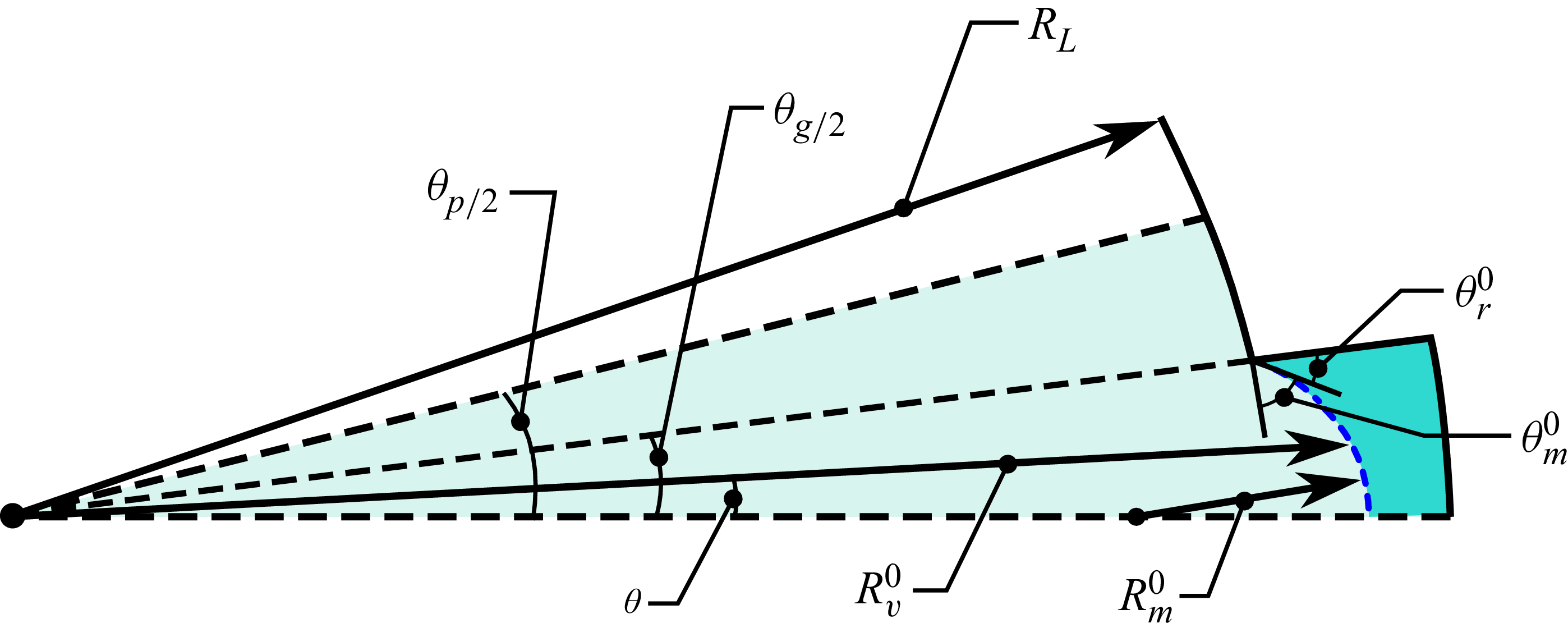
 ϵ

 θm=0
 N
 θ−θg/2
 |A^l|
 |C^n|
 l
 n
 O(1/l)
 O(1/n)

 |ξ~−ξ~series0|
 θm
 ∘
 ∘
 ∘
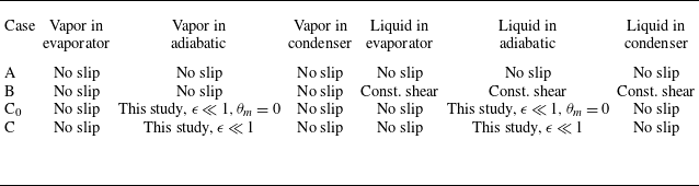
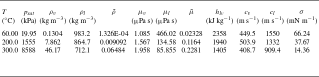
 c

 ξ~
 θm
 ϕ=0
 To∗
 ∘

 La∗
 Le∗=Lc∗
 To∗
 ∘
 Rg∗

 Le∗=Lc∗
 To∗
 ∘
 Rg∗

 Le∗=Lc∗
 To∗
 ∘
 Rg∗

 p∗
 z∗
 To∗
 ∘
 θm
 z∗

 vz,i∗
 ϕ=0∘
 To∗=60
 ∘
 θm=0∘
 ∘
 vz,i∗=0

 Vz,i0
 ∂Vz,v0/∂r
 θ
 ϕ=0
 To∗=60
 ∘

 fratio
 To
 Rg∗
 0
 θm=0
 θm=57∘

 ∘
 Rg∗
 La∗

 p∗
 z∗
 ϕ=90∘
 To∗
 ∘



