I. INTRODUCTION
Over the past several decades, significant progress has been made in understanding the dependency of bulk properties of polycrystalline materials on the grain boundary (GB) microstructure (Ref. Reference Aust and Chalmers1–Reference Wolf and Yip8). Based on this progress, grain boundary engineering (GBE) was proposed in early 1980s as an approach of optimizing boundary microstructures to achieve desired bulk properties,Reference Watanabe9 and has since been extensively studied and successfully implemented in many applications as summarized in two recent review articles.Reference Randle10,Reference Watanabe11 In addition to the GB, another interface component, the triple junction, has received more and more attention in interface studies and triple junction engineering has been introduced as one of the objectives in future GBE.Reference Watanabe11,Reference Gottstein and Shvindlerman12 This is due to their significant role in bulk properties demonstrated in previous studies on triple junctions as a topological structure connecting individual boundaries in polycrystalline materials (Ref. Reference Davies, Randle, Watkins and Davies13–Reference Rohrer, Randle, Kim and Hu16).
For example, it has been found that a polycrystalline wire containing triple junctions always displays higher ductility and lower strength than a wire without triple junctions having a bamboo grain structure.Reference Rabukhin17 Preferential corrosion at triple junctions was observed in high purity nickel for some electrochemical conditions.Reference Palumbo and Aust18 In the case of microstructural evolution, it has been shown that triple junctions can exert dragging forces on migrating boundaries during grain growth.Reference Gottstein, Sursaeva and Shvindlerman19–Reference Gottstein, Ma and Shvindlerman21 Regarding excess energy, thermal grooving at triple junctions on a free surface was found to be significantly deeper than at adjoining grain boundaries in several studies, indicating positive junction energy.Reference Mikhailovskii and Rabukhin22–Reference Zhao, Verhasselt, Shvindlerman and Gottstein24 However, thermodynamic calculation, modeling, and computer simulation suggested the existence of negative triple junction energy.Reference Srinivasan, Cahn, Jonsson and Kalonji25–Reference Upadhyay, Capolungo, Taupin and Fressengeas27 This contradiction between the experimental observation and theoretical calculation manifests the complex nature of triple junction structure, which has 11 macroscopic degrees of freedom in comparison to 5 for the GB structure.Reference King26 With the substantial increase of the triple junction volume fraction as the grain size decreases into the nanometer range,Reference Palumbo, Thorpe and Aust28,Reference Zhou, Erb and Aust29 triple junction effects are expected to be significant for the properties of nanocrystalline materials, as already demonstrated for mechanical properties,Reference Palumbo, Erb and Aust30 hydrogen diffusivity,Reference Palumbo, Doyle, El-Sherik, Erb and Aust31 mass transport,Reference Chellali, Balogh, Bouchikhaoui, Schlesiger, Stender, Zheng and Schmitz32 thermal stability,Reference Sherik, Boylan, Erb, Palumbo, Aust, Clark, Dahmen and Briant33 creep behavior,Reference Wang, Wang, Aust and Erb34 and structure relaxation.Reference Rupert, Trelewicz and Schuh35
Several analytical models have been proposed to describe triple junction microstructures. One of the earliest models was Bollmann’s I-line and U-line disclination model on the basis of the 0-lattice framework.Reference Bollmann36 In this model, the three adjoining grains are described by unique lattices to achieve the least lattice displacement between two adjacent grains, the so-called nearest neighbor relationships.Reference Bollmann37,Reference Bollmann38 Such grain structures result in two types of arrangement of dislocation arrays at triple junctions. In Type 1, the adjoining grain boundary dislocation (GBD) arrays form balanced nodes at the junction, whereas in Type 2, the crystallographic conditions of the adjoining GBD arrays preclude the establishment of a nodal balance, yielding a dislocation surplus (or deficit) and a higher energy at the triple junction line.Reference Bollmann39 Bollmann defined Type 1 structures as I-line triple junctions, whereas Type 2 junctions were termed U-line junctions, which have all the characteristics expected of disclinations.Reference Bollmann40
Since the triple junction is the meeting point of three boundaries, its structure can be characterized by defining the three adjoining GBs using the coincident site lattice (CSL) model.Reference Doni and Bleris41 This idea led to the CSL/GB model, whereby triple junctions are categorized into four groups according to the number of CSL boundaries among the three adjoining GB’s, i.e., 0, 1, 2, and 3, respectively.Reference Doni and Bleris41,Reference Kurzydlowski, Ralph and Garbacz42
Some degree of order may still exist in those triple junctions even though the nodal balance of the GBD arrays could not be formed (i.e., Bollmann’s U-line junctions) and/or none of the adjoining GB’s could be described by low Σ CSL relationships. To address this issue, Palumbo and AustReference Palumbo and Aust43 proposed the coincident axial direction (CAD) model. This model aimed to identify triple junctions having low index {h k l} atomic planes only slightly misaligned across the three adjoining lattices. Energetically, lattice relaxation may take place, leading to a region of perfect plane matching (PM) across the junction, upon which an array of intrinsic dislocations is superimposed and a one-dimensional periodicity proportional to the interplanar spacing is achieved along the triple junction line. Such triple junctions can be described by a Π value with Π = h 2 + k 2 + l 2, where [h k l] is the index of the CAD.Reference Palumbo and Aust43
Despite differences in the analytical methods, the aforementioned models require a common experimental approach: crystallographic orientation information to characterize triple junction microstructures in polycrystalline materials. Up to now, very few experimental studies have been performed to examine systematically the effectiveness of various triple junction models in an effort to correlate the junction microstructures with bulk properties.
Among the properties sensitive to the interface structure, chromium depletion due to carbide precipitation at grain boundaries is a well-studied phenomenon (Ref. Reference Aborn and Bain44–Reference Bruemmer49) because of its association with the detrimental intergranular corrosion in austenitic stainless steels (SSs) after certain heat treatments. Since intergranular attack has been observed to preferentially initiate at triple junctions (Ref. Reference Palumbo and Aust18), this detrimental degradation phenomenon could be significantly mitigated if an engineering process can be developed to modify the microstructure so that it contains a high fraction of special triple junctions with high resistance to the attack. A crucial step toward that goal is to develop a method to identify these special triple junctions.
In this study, carbide precipitation at triple junctions was investigated in Type 304L SS, whereby the junction structures were characterized by orientation imaging microscopy (OIM) associated with electron backscatter diffraction (EBSD) and analyzed using the models described above. The effectiveness of the models in identifying special junctions was examined through correlating the junction characters with their resistance to carbide precipitation. Details of characterizing junctions using the models are given in the Appendix.
II. EXPERIMENTAL
The material used in this work was commercial 304L SS; the concentrations for Ni, Cr, and Mn are determined by energy dispersive x-ray spectroscopy (EDS) and are given in Table I in wt%. For the other elements with content lower than the EDS resolution limit, are the maximum values provided by the material supplier (labeled with *).
Chemical composition of 304L SS in wt%.

Samples were cut from bulk 304L SS to a size approximately 6 × 6 × 2 (mm3) and then subjected to different heat treatment conditions. The objective of the heat treatment was to have carbide precipitation proceeding in a selective fashion so that possible triple junction structure differences, if any, would be revealed. The significance of selectivity has been well demonstrated in a previous study.Reference Palumbo and Aust50
In the current study, structure sensitivity to chromium depletion due to carbide precipitation was introduced by various degrees of sensitization treatments based on the time–temperature sensitization curves of carbide precipitation in different interface structures for 304 SS.Reference Stickler and Vinckier46 All samples were first solution treated, i.e., annealed at 1050 °C for 2 h to dissolve any residual carbides in the grain boundaries and triple junctions, followed by water quenching (WQ).Reference Stickler and Vinckier46 Then the samples were sensitized at different temperatures and/or times to induce varying amounts of carbide precipitation, thus different degrees of selectivity at triple junctions. All heat treatments were conducted in an argon atmosphere.
Subsequently, all samples were ground using silicon carbide grinding paper from 400 up to 2400 grit. They were mechanically polished sequentially using alumina with particle sizes of 3 μm down to 0.05 μm. The polished surfaces were then cleaned using ethanol to remove residual alumina particles. Then, the samples were electro-polished to obtain a deformation-free surface using a solution of 5 vol% percholic acid (70 vol% + 95 vol%) pure ethanol, at a current density of approximately 2.25 A/cm2 for 45 s at −20 °C. The final step was electro-etching to reveal carbide precipitation-induced intergranular pitting using an etchant of oxalic acid: water = 1(g):10(mL) at 3.6 V DC for 60 s at room temperature.Reference Gay and Vander Voort51
The crystallographic orientation was determined by EBSD analysis.Reference Randle52 EBSD measurements were performed in a Hitachi S-4500 scanning electron microscope (SEM; Hitachi Scientific Instruments, Tokyo, Japan) using an OIM system provided by TexSEM Laboratories. A step size of 1.5 μm was applied so as to ensure a minimum of three orientation measurements for each grain. This was based on SEM micrograph analysis showing that the smallest grains are about 5 μm in size for the material. Prior to the OIM analysis, the sample areas of interest were marked with microhardness indentations so that the same areas could be located easily under the electron microscope. Individual triple junctions were identified by matching the OIM maps with the corresponding SEM micrographs, and then characterized according to the various structural models. The number of analyzed junctions was 513 in total. Detailed procedures of a junction analysis are given in the Appendix.
III. RESULTS AND DISCUSSION
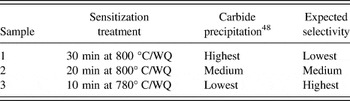
Table II summarizes the details of the sensitization treatments, qualitative estimation of the precipitation as well as the expected selectivity for each sample. Selectivity is crucial in GB structure–property investigations. In a study on the correlation between GB corrosion behavior and GB structure in high purity nickel, it was found that there were two characteristic overpotential curves, upper and lower curves, in a plot of GB corrosion potential versus sulfur concentration in nickel. The upper curve represented the lowest overpotential at which comprehensive intergranular corrosion at all GBs was observed, whereas complete immunity to intergranular corrosion at all GBs was observed at overpotentials below those defined by the lower curve. GB selectivity in the initiation of localized corrosion, i.e., structure-dependent GB corrosion, was only observed in the region bounded by these two curves.Reference Palumbo and Aust50
Sensitization treatment and expected selectivity.

In the current study, same sensitization treatments were applied because they have been proved to be effective in promoting selective precipitation upon interface structure as demonstrated in a previous study on carbide precipitation at GBs for 304 SS. For instance in a case of twin boundaries, the carbide precipitation was found to occur exclusively at incoherent twins, whereas no precipitation was observed at coherent twins.Reference Zhou, Erb, Aust and Palumbo53
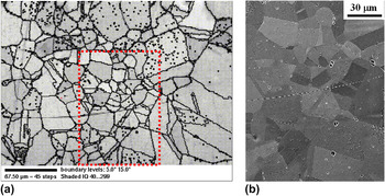
Figure 1 shows a representative OIM map and the SEM micrograph corresponding to one area in the map. Clearly, the map and the micrograph match very well, indicating that the step size of 5 μm is sufficiently fine to catch the orientation details of the specimen. In the map, a grain interior is defined as the area in which the misorientations vary by less than 5° among all measured points. Locations at which misorientations change by more than 5° are labeled as GBs.
(a) Representative OIM map and (b) SEM micrograph corresponding to the framed area in the map for a sensitized 304L sample.

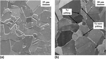
Figure 2 shows typical microstructures of electro-etched samples after (i) 2 h annealing at 1050 °C followed by WQ, i.e., the solution heat treatment (ST), and (ii) a sensitization heat treatment, i.e., ST + 20 min annealing at 800 °C followed by WQ.
Typical microstructures after etching for (a) solution-treated material with step-structure, and (b) sensitized material (ST + 20 min at 800 °C/WQ) with selective pitting at grain boundaries and triple junctions.

For the solution-treated sample, the step structure is the prevailing feature along GBs, indicating a sample free of carbide precipitation. Some randomly distributed pits were observed which are likely associated with random imperfections in the commercial 304L SS. On the other hand, the sensitized sample displayed extensive selective pitting at grain boundaries and triple junctions after being etched in oxalic acid [Fig. 2(b)], a typical phenomenon of intergranular pitting/corrosion due to carbide precipitation as demonstrated in previous studies in 304 SSs.Reference Aust47,Reference Kokawa, Shimada and Sato54,Reference Williford, Windisch and Jones55 While the susceptibility to carbide precipitation of various GB structures has been discussed elsewhere,Reference Zhou, Erb, Aust and Palumbo53 the following sections focus on the analysis of triple junction structures.
A. The I-line and U-line model
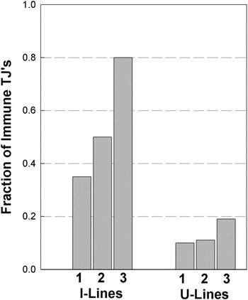
In this model, triple junctions are classified into two groups: I-line and U-line triple junctions. Figure 3 shows the fraction of triple junctions in the samples displaying immunity to carbide precipitation. In the case of I-lines, the fraction of immunity to carbide precipitation increases from 0.35 in Sample 1 and 0.5 in Sample 2 to 0.8 in Sample 3, whereas the fractions for U-lines are 0.10, 0.11, and 0.19 for Samples 1, 2, and 3, respectively.
Fractions of I-lines and U-lines, showing immunity to pitting in Samples 1, 2, and 3, respectively.

According to the structural description, I-lines are the triple junctions with a balanced GBD network.Reference Bollmann39 Energetically, they are expected to show some special or beneficial properties, such as higher resistance to carbide precipitation, in comparison to U-lines. But as demonstrated in previous studies, the existing special properties of a particular structure can be displayed only when the sample is properly prepared so that it is sensitive to the structure differences, showing a selective behavior. In the case of 304L SS, the selectivity depends on the sensitization conditions; longer time and/or higher temperature results in more severe carbide precipitation.Reference Stickler and Vinckier46 At the beginning of carbide formation, precipitation would be expected to proceed first in these GBs and triple junctions with the highest susceptibility. Higher selectivity would be expected for the samples with fewer precipitated carbides. As shown in Table II, the selectivity or the correlation between the triple junction structure and the susceptibility to carbide formation is expected to increase in a sequence of Samples 1, 2, and 3. This is actually demonstrated in Fig. 3. For Sample 1, I-line triple junctions displayed a low immunity fraction of only 0.35 to carbide precipitation. With the increasing selectivity, improvement of correlation was observed, and the immunity fractions increased to 0.50 for Sample 2 and 0.8 for Sample 3. The results indicate that the model is effective in identifying special triple junctions, i.e., I-lines.
In comparison, U-lines were described as triple junctions with dislocation surplus (or deficit), possessing higher energy,Reference Bollmann39 and thus can be expected to behave as preferential locations for carbide precipitation, showing high susceptibility/low immunity to precipitation. To a large extent, this is demonstrated in Fig. 3; carbide precipitation was observed in the majority of U-line triple junctions (more than 80%) for all three samples, regardless of sensitization conditions. Nonetheless, a certain number of U-line triple junctions still demonstrated immunity to precipitation with the fractions ranging from 0.1 to 0.19 (Fig. 3). This may be attributed to the fact that the characterization was performed assuming a rigid lattice structure surrounding a triple junction. In reality, structural relaxation may take place to form a lower energy configuration in a crystalline lattice. For example, in the case of CSL grain boundaries, small deviations from exact CSL misorientations can be accommodated by forming a secondary dislocation network through lattice relaxation so as to achieve a lower energy CSL configuration.Reference Grimmer, Bollmann and Warrington56 It may be possible that some apparent U-lines are able to form a balanced dislocation network, i.e., switch to I-lines, through structural relaxation in the vicinity across three adjoining grain lattices. Generally, such a relaxation would be easier for a U-line with less deviation from an exact I-line configuration. However, no specific quantitative criterion is currently available on the maximum allowable deviation for a triple junction switch from U-line to I-line character. Further work is required on a specific criterion for such derivations.
Overall, the behavior of carbide precipitation in this study agrees well with the results of a corrosion study in high purity nickel,Reference Palumbo and Aust18 in which it was found that corrosion pit initiation started mainly at U-lines. When the corrosion potential was increased, the pit initiation occurred at other sites, generally in the sequence of I-lines, grain boundaries and finally the crystal matrix. Based on these earlier and current experimental observations, it is reasonable to characterize I-lines as special triple junctions showing generally higher resistance to various forms of intergranular degradations than U-line triple junctions.
B. The CAD model
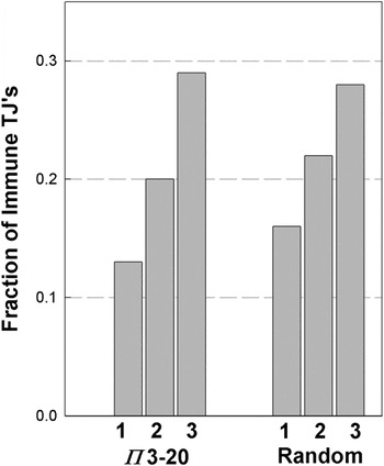
This model characterizes triple junctions based on a one-dimensional order parameter, a common axis across three adjoining grain lattices along the triple junction line.Reference Palumbo and Aust43 A certain degree of structural order is expected along the triple junction lines having a low index common axis or low Π value. The lowest six Π values are 3, 4, 8, 11, 19, and 20, corresponding to the common axes of <111>, <200>, <220>, <311>, <331>, and <420>. It has been shown that a randomly oriented polycrystalline material consists of approximately 30% of the triple junctions with a Π value between 3 and 20.Reference Fortier, Aust and Miller57 This percentage likely includes all the potentially beneficial junctions in a material with random texture. Hence, Π = 20 was set as the cut-off value for the special junctions in this study, and those with Π > 20 were classified as random junctions. In case that several low index axes common to three grains CAD were possible, the one with the lowest Π value was chosen for a triple junction. The angular deviation limit, ΔθCAD, for a special triple junction is given by ΔθCAD = 20.25 Π−1/2.Reference Randle and Ralph58Figure 4 shows the correlation between triple junction structures characterized according to the CAD model and the carbide precipitation behavior. Essentially, all characterized triple junctions, special and random ones, behave in a similar way. For Samples 1, 2, and 3, the fractions of the junctions showing immunity are 0.13, 0.20, and 0.29 for the special junctions, and 0.16, 0.22, and 0.28 for the random junctions, respectively. In all cases, more than 70% of the triple junctions are susceptible to carbide precipitation, regardless of the sensitization conditions.
Fractions of triple junctions characterized by the CAD model, showing immunity to pitting in Samples 1, 2, and 3, respectively.

Clearly, the model using the upper limit value of Π = 20 does not effectively identify the triple junctions exhibiting higher resistance to carbide precipitation. This may be attributed to the somewhat arbitrary criterion of Π = 20. If that is the case, the efficacy of the model should correspondingly increase when a stricter criterion is applied and fewer junctions are qualified as special junctions. For example, when the upper limit value of Π is lowered from 20 to 8, the number of qualified junctions is reduced from about 30% to about 5% in randomly textured materials,Reference Fortier, Aust and Miller57 and the efficacy of the model would be expected to improve. However, this turned out to be not the case for the precipitation behavior in this study. When the criterion of Π ≤ 8 was applied for special junctions, the fractions of the triple junctions with immunity to carbide precipitation remained essentially the same as for the case of Π ≤ 20. This suggests that a triple junction with just a one-dimensional order parameter, i.e., the common axial direction across three adjoining grains, has little structural advantage in demonstrating beneficial properties.
C. The CSL/GB model
In this model, the adjoining grain boundaries were characterized using the CSL approach; special grain boundaries were classified up to Σ29. Both Brandon’s criterion (BR, ΔθBR = 15 Σ−1/2)Reference Brandon59 and the Palumbo–Aust criterion (PA, ΔθPA = 15 Σ−5/6)Reference Palumbo and Aust50 were used for allowable deviations from the exact CSL boundary misorientations. Triple junctions were labeled according to the criterion used and the number of adjoining special grain boundaries. For example, BR2 represents a triple junction, having two special adjoining boundaries according to Brandon criterion, while PA1 describes a triple junction with 1 special boundary according to the Palumbo–Aust criterion.
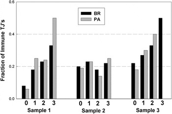
Figure 5 shows the effect of the number of adjoining special boundaries at triple junctions on carbide precipitation. Generally, triple junctions surrounded by a higher number of special boundaries are expected to have a more ordered structure, and thus stronger tendency to display beneficial properties. This is demonstrated in Samples 1 and 3, whereby triple junctions with a higher number of special boundaries show a higher likelihood of immunity to carbide precipitation. For instance, the frequency of immunity are 22% or less for those triple junctions without any adjoining special boundaries (BR0 and PA0), whereas the numbers increase to more than 33% and up to 50% when the triple junctions are surrounded by three special boundaries (BR3 and PA3). Note that no PA3 junctions were observed in Sample 3.
Fractions of triple junctions characterized by the CSL/GB model using both BR and PA criteria, showing immunity to pitting in Samples 1, 2, and 3, respectively.

The observation agrees with the results in previous studies, e.g., on the resistance to fatigue crackingReference Kobayashi, Inomata, Kobayashi, Tsurekawa and Watanabe60 and on the arrest of propagating cracksReference Hu, Xia, Li, Liu, Zhou, Chen and Wang61 for the TJ’s characterized by the same model.
However, the junctions in Sample 2 exhibited an inconsistent behavior; the immunity fraction varies in a narrow range between 0.14 and 0.25, independent of the adjoining GB characters. This inconsistency is surprising but may be understood when comparing with the results of another study, where a similar inconsistency was observed.Reference Kobayashi, Tsurekawa and Watanabe62 In that study, the hardening behavior of the GBs and TJs was investigated with respect to the grain interior in zone-refined high purity polycrystalline molybdenum. A consistent correlation was demonstrated for the hardening behavior of grain boundaries characterized by the CSL model; random GBs showed a higher degree of hardening than special GBs without exception. However, the correlation depended on the carbon content for the TJs characterized by the CSL/GB model. For a sample containing 3 ppm carbon, the junctions behaved as expected, and the degree of TJ hardening increases consistently with a higher number of random boundaries. But for a sample containing 14 ppm carbon, no consistent results were observed; the junction hardening behavior exhibited a random fashion and varied in a narrow range, independent of the TJ structural character. This inconsistency was attributed to the higher carbon content, indicating a strong sensitivity of the CSL/GB model toward the sample-to-sample variations in composition.Reference Kobayashi, Tsurekawa and Watanabe62
For the current study, the 304L SS samples contained multiple elements, e.g., C, P, and S (see Sec. II) that were in the 300–450 ppm nominal composition ranges. Among the three samples having the same global C content, different C contents in the state of solid solution and/or precipitation are expected after corresponding sensitization treatments (Table II). However, this difference is expected to have little contribution to the inconsistency observed in Sample 2, as long as the treatment promotes selective carbide precipitation, which is likely the case as indicated in the characterization using the I-line and U-line model. On the other hand, elements such as S and P can affect the energetic and kinetic aspects of precipitation because they have a high tendency to segregate in the interface regions. The total amount of these elements likely differed among various samples on a scale sufficient to compromise the efficacy of the CSL/GB model and resulted in the inconsistent behavior shown in Fig. 5. In other words, the current study provides another example, demonstrating the sensitivity of the CSL/GB model to the sample differences in chemical composition.
D. The PM/GB model
Given the complexity of the triple junction structure, it is possible that some features in junction microstructures useful in differentiating special from random junctions remain unidentified using the aforementioned three models. Another plausible way to characterize the triple junctions is to use an approach similar to the CSL/GB model, i.e., characterizing junctions by defining the three adjourning GB’s, but using a different method, the PM model,Reference Pumphrey63,Reference Loberg, Norden, Chadwick and Smith64 to describe the GB structures. Hence, the PM/GB model was introduced here as an additional method to characterize junctions. Similar to the CSL/GB model, triple junctions are classified into four groups according to the number of PM boundaries around a junction.
A Π value is assigned to describe the corresponding boundary, where Π is equal to h 2 + k 2 + l 2 and [h k l] is the matched plane normal index. Consistent with the choice in Sec. III. B, special boundaries were classified up to Π = 20, whereas boundaries with Π > 20 were classified as random. Slight deviations from exact PM are expected to be accommodated by grain boundary dislocation arrays. The deviation limit, ΔθPM, for a special boundary in f.c.c. materials is given by ΔθPM = 20.25 Π −1/2.Reference Randle and Ralph58 As in the case of the CSL/GB model, triple junctions were labeled according to the number of adjoining special grain boundaries. For example, PM2 represents a triple junction with two special adjoining boundaries characterized according to the PM model.
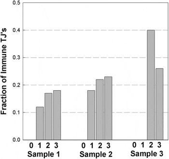
Figure 6 shows the resistance to pitting of different types of triple junctions according to the PM/GB model due to carbide precipitation. In Samples 1 and 2, the immunity to carbide precipitation increases slightly with decreasing sensitization time for the triple junctions with adjoining special boundaries (PM1, PM2, and PM3) and a higher number of adjoining special boundaries lead to higher immunity. For example, when the sensitization time decreases from 30 min (Sample 1) to 20 min (Sample 2), the immunity fraction for PM1 triple junctions increases from 0.12 (Samples 1) to 0.18 (Sample 2).
Fractions of triple junctions characterized by the PM/GB model, showing immunity to pitting in Samples 1, 2, and 3, respectively.

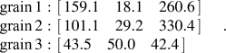
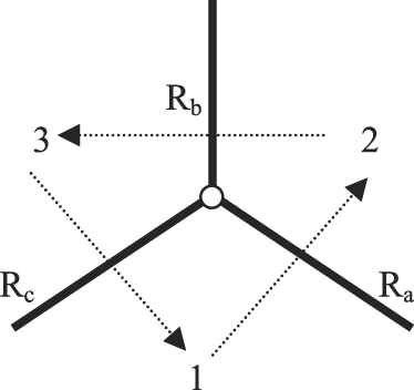
A schematic TJ with three grains, 1, 2, and 3, and three GBs, R a, R b, and R c. The arrows show the sequence of misorientation calculation. The three grain orientation data from a sample TJ in terms of three Euler angles with Bunge’s notation are:
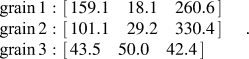 $$\matrix{ \matrix{ {\rm{grain \,}}1: \hfill \cr {\rm{grain }}\,2: \hfill \cr {\rm{grain }}\,3: \hfill \cr} \matrix{ \left[ {\matrix{ {159.1}\quad{18.1}\quad{260.6} \cr } } \right] \hfill \cr \left[ {\matrix{ {101.1}\quad{29.2}\quad{330.4} \cr } } \right] \hfill \cr \left[ {\matrix{ {43.5}\quad{50.0}\quad{42.4} \cr } } \right] \hfill \cr} \cr } \quad .$$
Regarding the number of special boundaries, the PM1, PM2, and PM3 triple junctions display a trend of increasing immunity fraction from 0.18, 0.22 to 0.23 in Sample 2. However, an inconsistency occurred in Sample 3, where a higher immunity fraction was observed for the junctions with two special boundaries (PM2 = 0.40) than those with three special boundaries (PM3 = 0.26). Overall, no group of triple junctions displayed a clear resistance against carbide precipitation, since the majority of the triple junctions (more than 60%) are susceptible to carbide precipitation in all four groups (PM0, PM1, PM2, and PM3). Evidently, the model failed to identify special triple junctions, i.e., those with high resistance to carbide precipitation, similar to the CAD model.
In the previous section, the failure of the CAD model has been attributed to the loose requirement for the junction microstructure, i.e., one-dimensional order, in identifying special triple junctions. As a matter of fact, the requirement is even less strict in the PM/GB model; it defines special triple junctions with one-dimensional order in the adjoining boundaries. According to a previous study,Reference Randle and Ralph58 the majority of GB’s (56%) in randomly textured polycrystals were special boundaries even with the stricter criterion of Π = 8 as the upper limit. At Π = 24, the probability of special boundaries increased to 73% in the GB character distribution.Reference Randle and Ralph58 Results from the CAD-related models suggest that they are not sufficient to effectively identify special triple junctions using characterization methods based on one-dimensional structural order.
On the other hand, the PM/GB model seems to have some merit in sorting out triple junctions with high randomness in their structures. None of the triple junctions with three random grain boundaries around them (PM0) showed immunity to carbide precipitation, regardless of the degree of selectivity. Likely, the PM0 triple junctions possess significant randomness in the structure as indicated by the lack of even one-dimensional order in any of their adjoining boundaries. These junctions are expected to be highly vulnerable to various interfacial degradation events such as precipitation, segregation, and corrosion.
E. Concluding comments
Among the four triple junction structure models discussed here, Bollmann’s disclination model is the most successful in identifying those triple junctions with high resistance to carbide precipitation. Excellent agreement was observed between the theoretical predictions and experimental results when the annealing condition approaches the proper selective region so that the carbide precipitation proceeds in a sequence from most to least vulnerable triple junction structures.
However, there has been considerable debate on the physical validity of Bollmann’s disclination model, in spite of the fact that the supporting experimental evidence was observed in previous studies.Reference Palumbo and Aust18,Reference Clarebrough and Forwood65 The focal point of the debate has been whether U-lines exist at all. Priester and YuReference Priester and Yu66 observed a Σ3–Σ3–Σ9 type triple junction using high-resolution microscopy. According to their calculation, it was a U-line; however they found that the nodal balance of dislocations occurred at this triple junction, which is the physical character of an I-line. As a result, they questioned the physical significance of the distinction between I-lines and U-lines. Later, Palumbo and AustReference Palumbo and Aust67 pointed out that the calculation performed by Priester and Yu on the triple junction was in error. The correct calculation showed that this Σ3–Σ3–Σ9 type triple junction was actually an I-line. In fact, this direct observation provides further support for the basic concepts of Bollmann’s disclination model.
The model was examined again by Dimitrakopulos et al.Reference Dimitrakopulos, Krakostas and Pond68 from the theoretical point of view. The key point in their argument was the validity of choosing a nearest-neighbor-relation (NNR), the cornerstone in Bollmann’s disclination model, in describing GB misorientations. For a given GB, the misorientation can be described in different mathematical expressions due to the symmetrical nature in crystalline lattices. They argued that all descriptions of a given boundary were equivalent and consistent with a physical bicrystal. A particular description (e.g., the NNR, corresponding to the widest spaced dislocation network) may be more convenient, but not more meaningful. When grain boundaries met at a triple junction, it was important to describe GB misorientations in a consistent manner. The NNR was obtained by an unimodular transformation, which would introduce inconsistency in describing adjoining GB misorientations at a triple junction. Therefore, choosing NNR was neither necessary nor valid as a criterion for the selection of GB misorientation descriptions at a triple junction. Without NNR, the sequence around a triple junction always leads to the I-line classification. Thus, they concluded that all triple junctions were I-lines in Bollmann’s terminology.
Later in another study,Reference Müllner69 it was pointed out that small angle tilt boundaries are made up by walls of edge dislocations with the smallest possible dislocation contentReference Read and Shockley70 and, thus, correspond to the NNR. In describing a virtual multiple junction (e.g., a triple junction), there are two approaches: (i) Bollmann’s disclination approach, in which the choice of the NNR is crucial as a criterion for selecting GB misorientation descriptions, and (ii) the conventional elasticity approach (rotational Volterra cuts, Volterra disclinations).Reference Romanov, Vladimirov and Nabarro71 Through a thought experiment, the author demonstrated that the Bollmann disclination, U-line, is a real crystallographic defect with the dislocation network corresponding to the NNR, and is physically different from the Volterra disclination (an elastic defect) in the second approach. Moreover, the Bollmann disclination (U-line) can only be identified by the first approach. The method used by Dimitrakopulos et al.Reference Dimitrakopulos, Krakostas and Pond68 in their work is the second approach (rotational Volterra cuts, Volterra disclination) and, hence, cannot identify the distinction between U-lines and I-lines.
The experimental results in this work have provided further support for the physical validity of Bollmann’s disclination model. Moreover, this work has also demonstrated that selectivity must be taken into consideration when assessing triple junction models with respect to properties, as was previously shown for GBs (Ref. Reference Palumbo and Aust50).
IV. SUMMARY
Bollmann’s I-line/U-line model gives the best fit for the experimental observations of carbide precipitation at triple junctions in sensitized Type 304L SS. The percentage of I-line triple junctions immune to the carbide precipitation reaches values up to 80% when the samples are annealed in the proper selective region. The percentage of U-line triple junctions immune to the carbide precipitation always remains below 20% under all annealing conditions investigated in this study. To a certain extent, the CSL/GB model functions as a capable method in characterizing special triple junctions against carbide precipitation. But the efficacy of the model likely depends on the impurity content and is very sensitive to sample-to-sample variations. The PM/GB model succeeds in identifying triple junctions with high randomness in their structure. All characterized random triple junctions displayed carbide precipitation regardless of annealing conditions. However, the PM/GB model is not sufficient in identifying the triple junctions with high resistance to carbide precipitation. No consistent correlation between triple junction structures and carbide precipitation was observed using the CAD model.
ACKNOWLEDGMENTS
Financial support from the Natural Sciences and Engineering Research Council of Canada (NSERC) and the Ontario Research Fund-Research Excellence (ORF-RE) is gratefully acknowledged.
APPENDIX - Triple junction characterization procedure
Here an example is presented to illustrate the calculation procedures of the four triple junction (TJ) models used in this study to determine the triple junction line characters.
First, the measured OIM orientation data are converted into rotation matrices, i.e., R1, R2, and R3 for grains 1, 2, and 3, respectively,
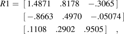 $$\eqalign{ R{\rm{1}} = \,\,\,\left[ {\matrix{ {1.4871} \quad{.8178} \quad{ - .3065} \cr } } \right] \cr\,\,\,\left[ {\matrix{ { - .8663} \quad{.4970} \quad{ - .05074} \cr } } \right] \cr\,\,\,\left[ {\matrix{ {.1108}\quad{.2902}\quad{.9505} \cr } } \right]\quad , \cr}$$
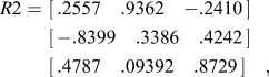 $$\eqalign{ R{\rm{2}} = \,\,\left[ {\matrix{ {{\rm{.2557}}} \quad{{\rm{.9362}}}\quad{ - {\rm{.2410}}} \cr } } \right] \cr \,\,\left[ {\matrix{ { - {\rm{.8399}}}\quad{{\rm{.3386}}} \quad{{\rm{.4242}}} \cr } } \right] \cr \,\,\left[ {\matrix{ {{\rm{.4787}}}\quad{{\rm{.09392}}}\quad{{\rm{.8729}}} \cr } } \right]\quad , \cr}$$
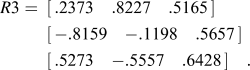 $$\eqalign{ R{\rm{3}} = \,\,\,\left[ {\matrix{ {{\rm{.2373}}} \quad{{\rm{.8227}}}\quad{{\rm{.5165}}} \cr } } \right] \cr \,\,\,\left[ {\matrix{ { - {\rm{.8159}}} \quad{ - {\rm{.1198}}} \quad{{\rm{.5657}}} \cr } } \right] \cr \,\,\,\left[ {\matrix{ {{\rm{.5273}}}\quad{{\rm{ - }}{\rm{.5557}}}\quad{{\rm{.6428}}} \cr } } \right]\quad . \cr}$$
Then the GB misorientations between two adjacent grains in reference to the crystal coordinates are calculated as follows (note that R −1 is an inverse matrix of R):
 $$R_a = R1^{ - 1} \,R2\,\,{\rm{ }}R_b = R2^{ - 1} {\rm{ }}\,\,R3\,\,{\rm{ }}R_c = R3^{ - 1} \,R1\quad ,$$
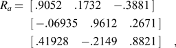 $$\eqalign{ R_a \,{\rm{ = }}\,\,\,\left[ {\matrix{ {{\rm{.9052}}}\quad{{\rm{.1732}}}\quad { - {\rm{.3881}}} \cr } } \right] \cr \;\;\left[ {\matrix{ { - {\rm{.06935}}}\quad{{\rm{.9612}}} \quad{{\rm{.2671}}} \cr } } \right] \cr \;\;\left[ {\matrix{ {{\rm{.41928}}}\quad{ - {\rm{.2149}}} \quad{{\rm{.8821}}} \cr } } \right]\quad , \cr}$$
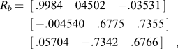 $$\eqalign{ R_b \,{\rm{ = }}\,\,\,\left[ {\matrix{ {{\rm{.9984}}}\quad{{\rm{04502 }}}\quad{ - {\rm{.03531}}} \cr } } \right] \cr \,\,\,\left[ {\matrix{ { - {\rm{.004540}}}\quad{{\rm{.6775}}} \quad{{\rm{.7355}}} \cr } } \right] \cr \,\,\,\left[ {\matrix{ {{\rm{.05704}}}\quad{ - {\rm{.7342}}}\quad{{\rm{.6766}}} \cr } } \right]\quad , \cr}$$
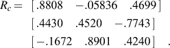 $$\!\!\!\eqalign{ R_c \,{\rm{ = }}\,\,\,\,\left[ {\matrix{ {{\rm{.8808}}}\quad { - .05836}\quad{{\rm{.4699}}} \cr } } \right] \cr \,\,\,\,\left[ {\matrix{ {{\rm{.4430}}} \quad{{\rm{.4520}}}\quad{ - .7743} \cr } } \right] \cr \,\,\,\,\left[ {\matrix{ { - {\rm{.1672}}}\quad{{\rm{.8901}}}\quad{{\rm{.4240}}} \cr } } \right]\quad . \cr}$$
Determination of TJ character using Bollmann’s model
The main idea in this model is to determine a unimodular matrix that leads to the nearest neighbor relation (NNR) with the adjacent grain. The starting point is the f.c.c. structure matrix S as the crystal unit cell,
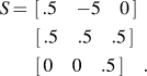 $$\eqalign{ S \,{\rm{ = }}\,\,\left[ {\matrix{ {.5}\quad{ - 5}\quad0 \cr } } \right] \cr\! \;\;\left[ {\matrix{ {.5}\quad{.5}\quad{.5} \cr } } \right] \cr\! \;\;\left[ {\matrix{ 0\quad0\quad{.5} \cr } } \right]\quad . \cr}$$
Convert the GB matrices with reference to the unit cell, e.g. R a, and get a new form of GB matrix, e.g. R a′
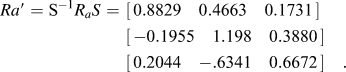 $$\eqalign{ Ra\prime = {\rm{S}}^{ - {\rm{1}}} R_a S \,\,{\rm{ = }}\,\,\left[ {\matrix{ {{\rm{0}}{\rm{.8829}}}\quad{{\rm{0}}{\rm{.4663}}}\quad {{\rm{0}}{\rm{.1731}}} \cr } } \right] \cr \,\,\left[ {\matrix{ { - {\rm{0}}{\rm{.1955}}}\quad{{\rm{1}}{\rm{.198}}}\quad{{\rm{0}}{\rm{.3880}}} \cr } } \right] \cr \,\,\left[ {\matrix{ {{\rm{0}}{\rm{.2044}}}\quad{ - {\rm{.6341}}}\quad {{\rm{0}}{\rm{.6672}}} \cr } } \right]\quad . \cr}$$
Then R a′ is decomposed into external (M_ext) and internal (M_int) matrix. The entries in the external matrix must be integers, whereas those in the internal matrix have values between 0 and 1 so that the column vectors in M_int are all inside the unit cell:
 $$\matrix{ {R_a \prime {\rm{ }}} {\rm{ = }} \,{M{\rm{\_ext}}} + {M{\rm{\_int}}} \cr \matrix{ \left[ {\matrix{ {{\rm{.8829}}}\quad{{\rm{.4663}}}\quad{{\rm{.1731}}} \cr } } \right] \hfill \cr \left[ {\matrix{ { - .1955}\quad {{\rm{1}}{\rm{.198}}}\quad{{\rm{.3880}}} \cr } } \right] \hfill \cr \left[ {\matrix{ {{\rm{.2044}}}\quad{ - {\rm{.6341}}}\quad{{\rm{.6672}}} \cr } } \right] \hfill \cr} = \matrix{ \left[ {\matrix{ 0 \quad0 \quad0 \cr } } \right] \hfill \cr \left[ {\matrix{ { - 1} \quad1 \quad0 \cr } } \right] \hfill \cr \left[ {\matrix{ 0 \quad{ - 1} \quad0 \cr } } \right] \hfill \cr} + \matrix{ \left[ {\matrix{ {{\rm{.8829}}}\quad{{\rm{.4663}}}\quad {{\rm{.1731}}} \cr } } \right] \hfill \cr \left[ {\matrix{ {{\rm{.8045}}}\quad{{\rm{.1984}}}\quad{{\rm{.3880}}} \cr } } \right] \hfill \cr \left[ {\matrix{ {{\rm{.2044}}}\quad{{\rm{.3659}}}\quad{{\rm{.6672}}} \cr } } \right] \hfill\quad . \cr} \cr } $$
The next step is to find the closest corner of the unit cell for each column vector in M_int. Since the unit cell coordinate is a nonorthonormal coordinate, the metric tensor G is required for the calculation of the (square) distance d i2 between a vector, v i, and a corner, c i,
 $$d_i ^{\rm{2}} = \Delta x_i ^{\rm{T}} Gx_i \quad ,$$
where G = S TS, and Δx i = v i − c i. The superscript T means the transpose of a vector or a matrix. Table A1 shows the results of d i2, whereby the minimum values of d 12, d 22, and d 32 (bold numbers) correspond to the corners of [1 1 0], [0 0 1], and [0 0 1], respectively. A matrix consisting of the corners of least distance, M_cor, is then constructed, using the corner coordinates as the column vectors, respectively,
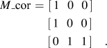 $$\eqalign{ M{\rm{\_cor}} \,\,{\rm{ = }}\,\,\left[ {\matrix{ 1\,\,\,\, 0\,\,\,\, 0 \cr } } \right] \cr \;\left[ {\matrix{ 1\,\,\,\, 0\,\,\,\, 0 \cr } } \right] \cr \;\left[ {\matrix{ 0\,\,\,\, 1\,\,\,\, 1 \cr } } \right]\quad . \cr}$$
Distances between internal vectors and unit cell corners.

Adding M_ext to M_cor leads to a reshaped unit cell, M_res. Note that the determinant of M_res has to be +1. Otherwise choose slightly larger values of di2 until the determinant is +1. In this case:
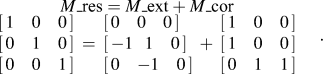 $$\matrix{ {M{\rm{\_res}}} = {M{\rm{\_ext}}} + {M{\rm{\_cor}}} \cr \matrix{ \left[ {\matrix{ 1\quad0\quad0 \cr } } \right] \hfill \cr \left[ {\matrix{ 0\quad 1\quad0 \cr } } \right] \hfill \cr \left[ {\matrix{ 0\quad0\quad1 \cr } } \right] \hfill \cr} = \matrix{ \left[ {\matrix{ 0\quad0\quad0 \cr } } \right] \hfill \cr \left[ {\matrix{ { - 1}\,\,\,\, 1\quad0 \cr } } \right] \hfill \cr \left[ {\matrix{ 0\quad { - 1}\quad0 \cr } } \right] \hfill \cr} + \matrix{ \left[ {\matrix{ 1\quad0\quad0 \cr } } \right] \hfill \cr \left[ {\matrix{ 1\quad0\quad 0 \cr } } \right] \hfill \cr \left[ {\matrix{ 0\quad1\quad1 \cr } } \right] \hfill \cr} \cr } \quad .$$
The unimodular matrix, U a, is then obtained for R a, the GB between grains 1 and 2 is given by
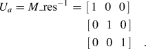 $$\eqalign{ U_a = M{\rm{\_res}}^{ - 1} \,\,{\rm{ = }}\,\,\left[ {\matrix{ 1\,\,\,\, 0\,\,\,\, 0 \cr } } \right] \cr \;\,\left[ {\matrix{ 0\,\,\,\, 1\,\,\,\, 0 \cr } } \right] \cr \;\,\left[ {\matrix{ 0\,\,\,\, 0\,\,\,\, 1 \cr } } \right]\quad . \cr}$$
Likewise, U b and U c can be derived as
 $$\matrix{ {U_b } \,\,{\rm{ = }}\!\!\! \matrix{ \left[ {\matrix{ 1\quad{ - 1}\quad{ - 1} \cr } } \right] \hfill \cr \left[ {\matrix{ 0\quad0\quad{ - 1} \cr } } \right] \hfill \cr \left[ {\matrix{ 0\quad1\quad1 \cr } } \right] \hfill \cr} {U_c }\quad{\rm{ = }}\!\!\! \matrix{ \left[ {\matrix{ 1\quad1\quad1 \cr } } \right] \hfill \cr \left[ {\matrix{ 0\quad1\quad1 \cr } } \right] \hfill \cr \left[ {\matrix{ 0\quad{ - 1}\quad0 \cr } } \right] \hfill \cr} \cr } \quad ,$$
and the TJ line character, T, can be readily determined as
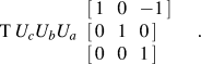 $$\matrix{ {\rm{T}} \,{U_c U_b U_a } \,\,\matrix{ \left[ {\matrix{ 1\,\,\,\, 0\,\,\,\, {- 1} \cr } } \right] \hfill \cr \left[ {\matrix{ 0\,\,\,\, 1\,\,\,\, 0 \cr } } \right] \hfill \cr \left[ {\matrix{ 0\,\,\,\, 0\,\,\,\, 1 \cr } } \right] \hfill \cr} \cr } \quad .$$
For this particular TJ, it is a U-line because T is not identity.
Determination of TJ character using the CSL/GB model
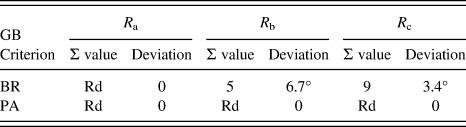
The OIM software is capable of identifying a CSL GB with Σ value using preset angle deviation allowance. In this study, two criteria were used for the deviation, namely, the Brandon criterion (BR) ΔθBR = 15° Σ−0.5 and the Palumbo–Aust criterion (PA) ΔθPA = 15° Σ−5/6. The results are shown in Table A2 for the same sample triple junction, where Rd stands for random.
Σ values of the three GBs using BR and PA criterion.
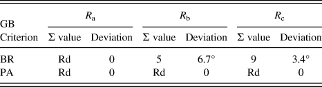
According to the BR criterion, the TJ has two CSL GBs, while it has no CSL GB using the PA criterion. Therefore, this is a BR2 or PA0 triple junction.
Determination of TJ character using the CAD model and the PM/GB model
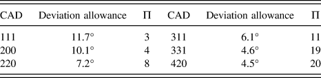
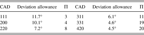
For both models, the first step is to construct a list of Π values and deviation allowances (ΔθCAD = 20.25 Π−0.5) as shown in Table A3.
The list of CAD and its Π value and deviation allowance.
Because of the symmetry, different misorientation matrices can be used to describe a given GB. It is crucial to use the matrix that gives the least rotation angle with the axis pointing into the standard stereographic triangle ([100], [110], [111]), the so-called disorientation matrix.
To do this, the trace (sum of the diagonal elements) of a GB matrix, e.g. R b, is maximized by interchanging rows and columns of the matrix. It results in R b_max:
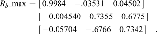 $$\eqalign{ R_b {\rm{\_max}} \,\,{\rm{ = }}\,\,\left[ {\matrix{ {{\rm{0}}{\rm{.9984}}}\quad{ - {\rm{.03531}}}\quad{{\rm{0}}{\rm{.04502}}} \cr } } \right] \cr \,\,\left[ {\matrix{ { - {\rm{0}}{\rm{.004540}}}\quad{{\rm{0}}{\rm{.7355}}}\quad{{\rm{0}}{\rm{.6775}}} \cr } } \right] \cr\,\, \left[ {\matrix{ { - {\rm{0}}{\rm{.05704}}}\quad{ - {\rm{.6766}}}\quad{{\rm{0}}{\rm{.7342}}} \cr } } \right]\quad . \cr}$$
Then R b_max is converted into angle-axis pair format,
 $${\rm{\theta }}\left[ {\matrix{ {{\rm{u,}}}\,\,\,\, {{\rm{v,}}}\,\,\,\, {\rm{w}} \cr } } \right] = 42.79^\circ \left[ {\matrix{ { - {\rm{43}}{\rm{.97}}}\,\,\,\, {{\rm{3}}{\rm{.314}}}\,\,\,\, {{\rm{1}}{\rm{.000}}} \cr } } \right]\quad .$$
The entries of the axis is re-arranged so that u ≥ v ≥ w ≥ 0 to obtain the axis pointing correctly. This leads to a new angle-axis pair:
 $$42.79^\circ \left[ {\matrix{ { {\rm{43}}{\rm{.97}}}\,\,\,\, {{\rm{3}}{\rm{.314}}}\,\,\,\, {{\rm{1}}{\rm{.000}}} \cr } } \right]\quad .$$
Converting the pair back into the matrix gives the disorientation matrix, R b_dis, between grains 2 and 3:
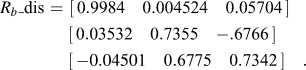 $$\eqalign{ R_b {\rm{\_dis}} \,\,{\rm{ = }}\,\,\left[ {\matrix{ {{\rm{0}}{\rm{.9984}}}\quad{{\rm{0}}{\rm{.004524}}}\quad{{\rm{0}}{\rm{.05704}}} \cr } } \right] \cr \;\left[ {\matrix{ {{\rm{0}}{\rm{.03532}}}\quad{{\rm{0}}{\rm{.7355}}}\quad{ - {\rm{.6766}}} \cr } } \right] \cr \;\left[ {\matrix{ { - 0.04501}\quad{{\rm{0}}{\rm{.6775}}}\quad{{\rm{0}}{\rm{.7342}}} \cr } } \right]\quad . \cr}$$
Beginning with CAD = [1, 1, 1] or Π = 3, grain 2 is taken as reference grain. So the CAD vector, V1, in grain 2, is V1 = [1, 1, 1], and the CAD vector, V2, in the adjacent grain (grain 3) is
 $$V{\rm{2}} = R_b {\rm{\_dis}}V{\rm{1}} = [1.060,0.09424,1.367]\quad .$$
The angle, θb, between V1 and V2, is obtained using the vector scalar product:
 $$V{\rm{1}} \cdot V{\rm{2}} = {\rm{|}}V{\rm{1| |}}V{\rm{2| cos}}\theta _b \quad .$$
So θb = 32.82°, which is larger than the deviation allowance, i.e., 11.7° (see Table A3). Moving on to Π = 4 or CAD = [2, 0, 0], and repeating the procedure gives V1 = [2, 0, 0], and V2:
 $$V{\rm{2}} = R_b {\rm{\_dis }}\,V{\rm{1}} = {\rm{[}}1.997,0.07064, - .09002{\rm{]}}\quad .$$
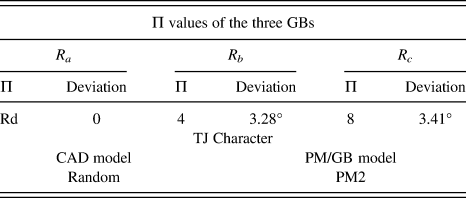
Since θb = 3.28°, smaller than 10.1° (see Table A3), this is a Π4 GB. Likewise, R c is found to be a Π8 GB with the deviation angle of 3.41°, while R a is a random GB because all its deviation angles up to Π = 20 are greater than the allowances. The results are summarized in Table A4.
TJ characters of the CAD and PM/GB models.
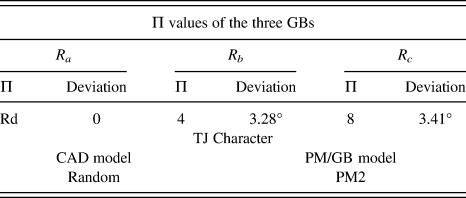
Therefore, according to the CAD model, the triple junction is a random TJ since no common Π ≤ 20 value is found among three GBs.
The same TJ is defined as a PM2 triple junction because it has two special GBs, Π8 and Π4 according to the PM/GB model (Table A4).