2 Mathematical model

An incompressible inviscid-limit, axisymmetric swirling flow in a finite-length circular pipe with a diverging or contracting geometry is studied. All distances are scaled with the pipe inlet radius, $R_{i}$ . The cylindrical coordinates $(r,\unicode[STIX]{x1D703},x)$ are used where $r$ is the non-dimensional radial distance from the centreline, $x$ is the non-dimensional axial distance from the inlet section and $\unicode[STIX]{x1D703}$ is the azimuth angle, $0\leqslant \unicode[STIX]{x1D703}<2\unicode[STIX]{x03C0}$ . The pipe non-dimensional length is $L$ . The non-dimensional pipe geometry is given by $R(x)=1+\unicode[STIX]{x1D70E}R_{0}(x)$ for $0\leqslant x\leqslant L$ , where $\unicode[STIX]{x1D70E}$ is a measure of the pipe divergence for positive values of $\unicode[STIX]{x1D70E}$ or contraction for $-1<\unicode[STIX]{x1D70E}<0$ . The case of $\unicode[STIX]{x1D70E}=0$ represents a straight pipe. The function $R_{0}(x)$ describes the pipe monotonic shape with the following conditions; at the inlet $R_{0}(0)=0$ , along the pipe $0\leqslant R_{0}(x)\leqslant 1$ and $(\text{d}R_{0}/\text{d}x)>0$ for $0\leqslant x<L$ and the pipe shape slope vanishes at the outlet, $(\text{d}R_{0}/\text{d}x)(L)=0$ . In this cylindrical system, we define $(u,v,w)$ as the non-dimensional radial, azimuthal and axial velocity components, respectively, where the velocity components are scaled with the characteristic axial speed entering the pipe, $U$ . The time $t$ is scaled with the ratio of pipe radius to inlet characteristic speed, $R_{i}/U$ . We define $y=r^{2}/2$ . From the assumed axisymmetry, a streamfunction $\unicode[STIX]{x1D713}(x,y,t)$ is used, where $u=-\unicode[STIX]{x1D713}_{x}/\sqrt{2y}$ and $w=\unicode[STIX]{x1D713}_{y}$ . The reduced azimuthal vorticity is

where the azimuthal vorticity is $\unicode[STIX]{x1D702}=\sqrt{2y}\unicode[STIX]{x1D712}$ . The circulation function is defined by $K=rv=\sqrt{2y}v$ . The unsteady axisymmetric circulation–vorticity equations which relate the evolution of $\unicode[STIX]{x1D713}(x,y,t)$ , $\unicode[STIX]{x1D712}(x,y,t)$ and $K(x,y,t)$ in the domain $0\leqslant x\leqslant L$ and $0\leqslant y\leqslant R^{2}(x)/2$ are described by:

Equation (2.2a ) describes the transport of flow circulation along a path line. Equation (2.2b ) represents the interaction between the transport of the reduced azimuthal vorticity $\unicode[STIX]{x1D712}$ along a path line and the stretching of vorticity by the axial gradient of the circulation. The stretching effect depends on swirl and may induce global azimuthal vorticity disturbances in the pipe that can propagate either downstream or upstream. These waves may be more pronounced along the centreline or the wall. They may interact with the inlet vortex generator device and the outlet passive discharge in a finite time to grow in size and evolve into states with separation zones.

To mimic experimental set-ups, the system (2.1)–(2.2) is solved under certain boundary conditions. We study the case of a setting where the inlet profile is a steady solid-body rotating flow with a uniform axial velocity, i.e. for all time $t\geqslant 0$ and for $0\leqslant y\leqslant 1/2$ , $\unicode[STIX]{x1D713}(0,y,t)=\unicode[STIX]{x1D713}_{0}(y)=y$ and $K(0,y,t)=2\unicode[STIX]{x1D714}y$ . Here $\unicode[STIX]{x1D714}\geqslant 0$ is the inlet flow swirl ratio. The reduced azimuthal vorticity at the inlet is set to be $\unicode[STIX]{x1D712}(0,y,t)=-\unicode[STIX]{x1D713}_{0yy}=0$ which results in the condition $\unicode[STIX]{x1D713}_{xx}(0,y,t)=0$ along the inlet for all times $t\geqslant 0$ and $0\leqslant y\leqslant 1/2$ . We emphasize that the radial velocity along the inlet is not prescribed and can change in time to describe the interaction between the inlet state and the propagation of waves in the pipe.

As was stated in Rusak & Wang (Reference Rusak and Wang2014), these inlet conditions may represent the nature of the rolled-up vortex flow behind a vortex generator that consists of a specifically designed system of fixed-in-time and fixed-in-space guiding (turning) vanes with special flow resistances through the vanes and a conical centre body. See for example, the experimental apparatus of Umeh et al. (Reference Umeh, Rusak, Gutmark, Villalva and Cha2010) who used a triple annular research swirler to generate a near-solid-body rotation flow with a near-uniform axial velocity (except near the wall). We also refer to Snyder & Spall (Reference Snyder and Spall2000), who demonstrated that a numerical simulation of the flow in a pipe including the guiding vanes system ahead of it and a simulation of the flow in the pipe alone, with fixed-in-time inlet axial and circumferential velocity profiles taken from the full apparatus simulation, give the same results and both resemble the experiments of Sarpkaya (Reference Sarpkaya1974).

We also note that the inlet conditions with zero azimuthal vorticity form at the inlet, at a fixed $\unicode[STIX]{x1D714}$ , a conserved total head $H$ that is the same for all solutions found at that $\unicode[STIX]{x1D714}$ , i.e. $H(0,r)$ does not change with the solution of the flow inside the domain even though the solution may exhibit a non-zero radial velocity $u(0,r)$ at the inlet. Therefore, this set of pipe inlet conditions describes for all $\unicode[STIX]{x1D714}$ a total head-conserving apparatus which can be physically realized. On the other hand, the inlet condition with vanishing radial velocity used by Leclaire & Sipp (Reference Leclaire and Sipp2010) does not conserve the total head and changes with the solutions at the same $\unicode[STIX]{x1D714}$ . We refer for details to Appendix A of Wang & Rusak (Reference Wang and Rusak2011).

The boundary condition at the pipe outlet describes a state with zero radial velocity (parallel flow state) all along the outlet, i.e. for all time $t\geqslant 0$ , $\unicode[STIX]{x1D713}_{x}(L,y,t)=0$ for $0\leqslant y\leqslant R^{2}(L)/2$ . For a sufficiently long pipe, where $L\geqslant 6$ , this condition reflects the experimental data of Umeh et al. (Reference Umeh, Rusak, Gutmark, Villalva and Cha2010) where at various swirl levels the mean flow formed a parallel flow state at a distance of approximately six radii from the inlet.

The condition of axisymmetry is applied along the centreline, i.e. $\unicode[STIX]{x1D713}(x,0,t)=0$ for $0\leqslant x\leqslant L$ and for all time $t\geqslant 0$ .

In the inviscid-limit flow formulation, the streamfunction is fixed along the pipe wall at $y=R^{2}(x)/2$ , i.e. $\unicode[STIX]{x1D713}(x,R^{2}(x)/2,t)=1/2$ for $0\leqslant x\leqslant L$ and all times $t\geqslant 0$ . It describes a constant volumetric flux across the pipe and the tangent flow condition to the wall all along the pipe wall. As long as the flow is with no wall separation and at high $Re$ , and the wall boundary layer stays thin, there is only a small influence of the thin wall boundary layer on the flow in the bulk. This is true for both diverging and contracting pipes as well as when centreline breakdown zones appear. When wall-separation zones appear in the swirling flow, they are characterized by zero radial and axial velocities and there is no axial velocity boundary layer attached to the wall. However, the circulation in the zone stays constant. Therefore, in a diverging pipe, the circumferential velocity decreases inside this zone and the circumferential boundary layer is not significant and decreases in its size. On the other hand, when the pipe is contracting, the circumferential velocity increases inside this zone and the circumferential boundary layer becomes more significant, yet small in size, when $Re$ is high. We conjuncture that in all flow cases there is only a small influence of the axial and circumferential velocity boundary layers on the flow in the bulk.

The set of assumed boundary conditions is consistent with the unsteady transport equations (2.2) and with the Poisson equation (2.1) for the streamfunction $\unicode[STIX]{x1D713}$ in terms of $\unicode[STIX]{x1D712}$ . These conditions form a well-posed problem of the flow evolution in the pipe. The problem may represent the inviscid-flow limit behaviour of high- $Re$ flows in a pipe. Given the initial conditions $\unicode[STIX]{x1D713}(x,y,0)$ , $K(x,y,0)$ and $\unicode[STIX]{x1D712}(x,y,0)$ , it describes the axisymmetric dynamics of a swirling flow in a finite-length diverging or contracting pipe. In addition, the inlet vorticity condition forms a base case where the total head and circulation functions entering the pipe are the same for multiple possible steady states in the pipe at the same swirl and with the same boundary conditions (see discussion in the appendix A in Wang & Rusak Reference Wang and Rusak2011). We note that Rusak (Reference Rusak1998) studied the effect of a non-zero inlet azimuthal vorticity ( $\unicode[STIX]{x1D712}(0,y,t)=\unicode[STIX]{x1D70F}(y)\neq 0$ ). It was found that such an effect creates imperfection on the bifurcation diagram of steady-state solutions for $\unicode[STIX]{x1D712}(0,y,t)=0$ . Therefore, the case with $\unicode[STIX]{x1D712}(0,y,t)=0$ forms a base case study where only the effect of geometry is considered.

Similar boundary conditions were applied by Beran & Culick (Reference Beran and Culick1992), Beran (Reference Beran1994), Lopez (Reference Lopez1994), Ruith et al. (Reference Ruith, Chen, Meiburg and Maxworthy2003) and Gallaire & Chomaz (Reference Gallaire and Chomaz2004) in their viscous flow numerical simulations of swirling flows in a pipe and by Buntine & Saffman (Reference Buntine and Saffman1995), Wang & Rusak (Reference Wang and Rusak1997a ), Leclaire & Sipp (Reference Leclaire and Sipp2010), Rusak et al. (Reference Rusak, Wang, Xu and Taylor2012) and Rusak & Wang (Reference Rusak and Wang2014) in their studies of inviscid swirling flows in a pipe.

We also emphasize that in the present flow set-up there is no necessary symmetry between the relatively fixed flow conditions at the pipe inlet and the relatively passive flow conditions at the outlet. This axial asymmetry generates an active role of the inlet and outlet flow states in determining the flow structure in the pipe (Wang & Rusak Reference Wang and Rusak1997a , Reference Wang and Rusak2011; Gallaire & Chomaz Reference Gallaire and Chomaz2004). It forms a dynamic axial inhomogeneity of the convective flow along the pipe which results in the appearance of large axial and radial changes of the flow structure from a parallel (or a near-parallel) flow state, specifically when the swirl is close to the critical level $\unicode[STIX]{x1D714}_{1}$ . Pipe divergence or contraction induces an additional axial inhomogeneity which affects or even dominates the flow evolution in the pipe.

The flow evolution according to the unsteady problem (2.1)–(2.2) and assumed boundary conditions is solved numerically using the algorithm described in appendix A. The simulations follow the algorithm of Xu (Reference Xu2012) and Rusak et al. (Reference Rusak, Wang, Xu and Taylor2012) for inviscid flow simulations in a straight pipe. A transformation of coordinates $\bar{x}=x,~\bar{y}=y/R^{2}(x)$ is used in the present study to convert the physical flow domain of a diverging or contracting pipe into a rectangular computational domain and to rewrite (2.1)–(2.2) in terms of the transformed coordinates. A first-order forward difference in time and a second-order upwind finite difference scheme in space are used to integrate $K$ and $\unicode[STIX]{x1D712}$ in time. A second-order central difference scheme is used to integrate $\unicode[STIX]{x1D713}$ in terms of $\unicode[STIX]{x1D712}$ . The time step must obey certain criteria to guarantee numerical stability of the computations. The results of flow evolution for various $\unicode[STIX]{x1D70E}$ and $\unicode[STIX]{x1D714}$ , specifically the resulting time-asymptotic states, are compared in § 5 with predictions according to theoretical considerations derived in §§ 3 and 4.

3 Analysis of steady states

We look to establish the bifurcation diagram of steady-state solutions of the unsteady problem (2.1) and (2.2) with the prescribed boundary conditions as the inlet swirl ratio $\unicode[STIX]{x1D714}$ is increased from zero to higher values for a fixed pipe geometry.

4 Solutions of the columnar SLE problem

The columnar SLE problem (3.7) with (3.8) may have several types of solutions. The base type is denoted as type $0$ and exists only for $\unicode[STIX]{x1D70E}=0$ (for which the outlet radius is $R(L)=1$ ). It is described by a streamfunction $\unicode[STIX]{x1D713}_{c}(y)=y$ , for which the axial velocity is $\unicode[STIX]{x1D713}_{cy}(y)=1$ and the pressure is $p_{c}(y)=1+\unicode[STIX]{x1D714}^{2}y$ . This solution is also the base columnar state of a solid-body rotation flow in a straight $(\unicode[STIX]{x1D70E}=0)$ pipe and exists for all $\unicode[STIX]{x1D714}$ , i.e. $\unicode[STIX]{x1D713}_{s}(x,y)=y$ . For this base state, $E(\unicode[STIX]{x1D713}_{c};\unicode[STIX]{x1D714};\unicode[STIX]{x1D70E}=0)=1+\unicode[STIX]{x1D714}^{2}/8$ and ${\mathcal{E}}(\unicode[STIX]{x1D713}_{s};\unicode[STIX]{x1D714};\unicode[STIX]{x1D70E})=(1+\unicode[STIX]{x1D714}^{2}/8)L$ .

Type $1$ solution is characterized by $0<\unicode[STIX]{x1D713}_{cy}(0)<1$ , where the centreline axial velocity $\unicode[STIX]{x1D713}_{cy}(0)$ is unknown and must be found as part of solution iterations until convergence with the wall condition $\unicode[STIX]{x1D713}_{c}((1+\unicode[STIX]{x1D70E})^{2}/2)=1/2$ is achieved. For this solution, from Bernoulli’s law along the pipe centreline connecting between the inlet and the outlet states, the centreline pressure is $p_{c}(0)=3/2-\unicode[STIX]{x1D713}_{cy}^{2}(0)/2>1$ . 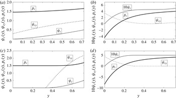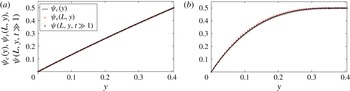An example of a type $1$ solution for a diverging pipe with $\unicode[STIX]{x1D70E}=0.2$ (for which the outlet radius is $R(L)=1.2$ ) and inlet swirl ratio $\unicode[STIX]{x1D714}=1$ is shown in figure 1(a). For this case the centreline axial velocity is $\unicode[STIX]{x1D713}_{cy}(0)=0.295$ . The streamfunction $\unicode[STIX]{x1D713}_{c}(y)$ , the axial velocity $\unicode[STIX]{x1D713}_{cy}(y)$ and the pressure $p_{c}(y)$ are monotonically increasing with $y$ . For a long pipe, type $1$ solutions of the columnar SLE problem (3.7) and (3.8) correspond to solutions of the SLE (PDE) problem (3.4) and (3.5) that describe a decelerated flow around the centreline all along the pipe.

Figure 1.

Four types of solutions of the columnar SLE problem (3.7) with (3.8). Here pipe is diverging with $\unicode[STIX]{x1D70E}=0.2$ . (a) Type $1$ is a solution with $0<\unicode[STIX]{x1D713}_{cy}(0)<1$ ; solution shown is for $\unicode[STIX]{x1D714}=1$ . (b) Type $2$ is a solution with $\unicode[STIX]{x1D713}_{cy}(0)>1$ ; solution shown is for $\unicode[STIX]{x1D714}=2$ . (c) Type $3$ is a solution with a centreline stagnation zone; solution shown is for $\unicode[STIX]{x1D714}=2$ . (d) Type $4$ is a solution with a wall quasi-stagnation zone; solution shown is for $\unicode[STIX]{x1D714}=2$ . In each panel, $\unicode[STIX]{x1D713}_{c}(y)$ is the streamfunction solution of the columnar SLE problem (3.7) with (3.8) (the thin solid line), $\unicode[STIX]{x1D713}_{cy}(y)$ is the resulting axial velocity (the dashed line) and $p_{c}(y)$ is the resulting pressure distribution according to (3.10) (the heavy solid line).

Type $2$ solution is characterized by $\unicode[STIX]{x1D713}_{cy}(0)>1$ , where again the centreline axial velocity $\unicode[STIX]{x1D713}_{cy}(0)$ is unknown and found as part of solution iterations until convergence with $\unicode[STIX]{x1D713}_{c}((1+\unicode[STIX]{x1D70E})^{2}/2)=1/2$ is achieved. For this solution, the centreline pressure is $p_{c}(0)=3/2-\unicode[STIX]{x1D713}_{cy}^{2}(0)/2<1$ . An example of a type $2$ solution for a diverging pipe with $\unicode[STIX]{x1D70E}=0.2$ ( $R(L)=1.2$ ) and inlet swirl ratio $\unicode[STIX]{x1D714}=2$ is shown in figure 1(b). Here the centreline axial velocity is $\unicode[STIX]{x1D713}_{cy}(0)=3.457$ . In this case, the streamfunction $\unicode[STIX]{x1D713}_{c}(y)$ and pressure $p_{c}(y)$ are monotonically increasing with $y$ , but the axial velocity $\unicode[STIX]{x1D713}_{cy}(y)$ reaches a minimum at $y\sim 0.4$ . For a long pipe, type $2$ solutions of the columnar SLE problem (3.7) and (3.8) correspond to solutions of the SLE (PDE) problem (3.4) and (3.5) that describe an accelerated flow around the centreline all along the pipe.

Type $3$ solution is characterized by a stagnation zone around the centreline with $\unicode[STIX]{x1D713}_{c}(y)=\unicode[STIX]{x1D713}_{cy}(y)=0$ for $0\leqslant y\leqslant y_{0}$ , where the size of the zone satisfies $0<y_{0}<(1+\unicode[STIX]{x1D70E})^{2}/2$ and is unknown and must be found as part of solution iterations until convergence with the wall condition $\unicode[STIX]{x1D713}_{c}((1+\unicode[STIX]{x1D70E})^{2}/2)=1/2$ is achieved. The solution of the columnar SLE (3.7) with (3.8) is sought in the range $y_{0}\leqslant y\leqslant (1+\unicode[STIX]{x1D70E})^{2}/2$ with continuous interface conditions $\unicode[STIX]{x1D713}_{c}(y_{0})=\unicode[STIX]{x1D713}_{cy}(y_{0})=0$ . In addition, from Bernoulli’s law along the pipe centreline, the centreline pressure is $p_{c}(y)=3/2$ for the whole range $0\leqslant y\leqslant y_{0}$ and the initial condition for pressure equation is $p_{c}(y_{0})=3/2$ . An example of a type $3$ solution for a diverging pipe with $\unicode[STIX]{x1D70E}=0.2$ and inlet swirl ratio $\unicode[STIX]{x1D714}=2$ is shown in figure 1(c). Here we find that $y_{0}=0.332$ . In the stagnation zone around the centreline, the streamfunction is zero, $\unicode[STIX]{x1D713}_{c}(y)=0$ , the axial velocity is zero, $\unicode[STIX]{x1D713}_{cy}(y)=0$ and pressure is constant, $p_{c}(y)=3/2$ . The streamfunction $\unicode[STIX]{x1D713}_{c}(y)$ , the axial velocity $\unicode[STIX]{x1D713}_{cy}(y)$ and the pressure $p_{c}(y)$ increase monotonically outside the stagnation zone. Specifically, the axial velocity grows from zero at the stagnation zone interface to above $1$ near the wall to maintain same volumetric flux as that at the inlet. For a long pipe, type $3$ solutions of the columnar SLE problem (3.7) and (3.8) represent solutions of the SLE (PDE) problem (3.4) and (3.5) with an outlet that contains a finite-size stagnation zone around the centreline of radial width $\sqrt{2y_{0}}$ . These solutions correspond to steady vortex-breakdown states of the SLE (PDE) problem with a centreline stagnation zone that starts inside the domain.

Type $4$ solution is characterized by a quasi-stagnation zone with $\unicode[STIX]{x1D713}_{c}(y)=1/2$ and $\unicode[STIX]{x1D713}_{cy}(y)=0$ for the range $y_{w}\leqslant y\leqslant (1+\unicode[STIX]{x1D70E})^{2}/2$ , where the zone size satisfies $0<y_{w}<(1+\unicode[STIX]{x1D70E})^{2}/2$ and is unknown and must be found as part of solution iterations. The solution of the columnar SLE is sought in the range $0\leqslant y\leqslant y_{w}$ with continuous interface conditions $\unicode[STIX]{x1D713}_{c}(y_{w})=1/2$ and $\unicode[STIX]{x1D713}_{cy}(y_{w})=0$ . In this case the equation is integrated backwards from $y_{w}$ to zero with repeated iterations until the centreline condition $\unicode[STIX]{x1D713}_{c}(0)=0$ is satisfied. It should be clarified that the axial and radial velocities are zero in the range $y_{w}\leqslant y\leqslant (1+\unicode[STIX]{x1D70E})^{2}/2$ . However, the circulation and the circumferential velocity do not vanish in this range. There, $K(y)=\unicode[STIX]{x1D714}$ and $v(y)=\unicode[STIX]{x1D714}/\sqrt{2y}$ . The interface pressure $p_{c}(y_{w})$ for a type $4$ solution is determined in the following way. Along the pipe wall $H(1/2)=3/2+\unicode[STIX]{x1D714}^{2}$ and $K(1/2)=\unicode[STIX]{x1D714}$ . Then, $v((1+\unicode[STIX]{x1D70E})^{2}/2)=\unicode[STIX]{x1D714}/(1+\unicode[STIX]{x1D70E})$ and $v(y_{w})=\unicode[STIX]{x1D714}/\sqrt{2y_{w}}$ . From Bernoulli’s law along the streamline $\unicode[STIX]{x1D713}=1/2$ connecting the inlet wall to $y=y_{w}$ at the outlet, we find that the interface pressure is $p_{c}(y_{w})=H(1/2)-(1/2)v^{2}(y_{w})=3/2+\unicode[STIX]{x1D714}^{2}-\unicode[STIX]{x1D714}^{2}/4y_{w}$ . An example of a type $4$ solution for a diverging pipe with $\unicode[STIX]{x1D70E}=0.2$ and inlet swirl ratio $\unicode[STIX]{x1D714}=2$ is shown in figure 1(d). Here we find that $y_{w}=0.300$ . In the wall quasi-stagnation zone, $\unicode[STIX]{x1D713}_{c}(y)=1/2$ , the axial velocity is zero, $\unicode[STIX]{x1D713}_{cy}(y)=0$ , but the pressure is not constant. Outside the zone, the streamfunction $\unicode[STIX]{x1D713}_{c}(y)$ and pressure $p_{c}(y)$ are monotonically increasing and the axial velocity is decreasing with the increase of $y$ . For a long pipe, type $4$ solutions of the columnar SLE problem (3.7) and (3.8) represent solutions of the SLE (PDE) problem (3.4) and (3.5) with an outlet state that contains a finite-size, zero axial and zero radial velocity, (quasi-stagnation) zone attached to the pipe wall. These solutions correspond to steady wall-separation states of the SLE (PDE) problem with a wall quasi-stagnation zone that starts inside the domain.

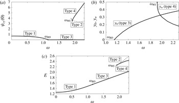
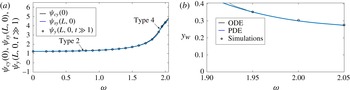
The results of successive computations for a diverging pipe with $\unicode[STIX]{x1D70E}=0.2$ in the range of inlet swirl ratio $0\leqslant \unicode[STIX]{x1D714}\leqslant 2.3$ are summarized in the bifurcation diagram of solutions of the columnar SLE problem, see figure 2. In figure 2(a), the horizontal axis is the inlet swirl ratio $\unicode[STIX]{x1D714}$ and the vertical axis is the value of the centreline axial velocity $\unicode[STIX]{x1D713}_{cy}(0)$ of each solution type. This is a representative parameter of the various solutions.

Figure 2.

Bifurcation diagrams of solutions of the columnar SLE problem (3.7) with (3.8) for a diverging pipe with $\unicode[STIX]{x1D70E}=0.2$ and the range of swirl ratio $0\leqslant \unicode[STIX]{x1D714}\leqslant 2.3$ . (a) $\unicode[STIX]{x1D713}_{cy}(0)$ of the various solution types as a function of $\unicode[STIX]{x1D714}$ ; (b) separation zone sizes $y_{0}$ (for type $3$ solutions) and $y_{w}$ (for type $4$ solutions) as a function of $\unicode[STIX]{x1D714}$ ; (c) $E$ as a function of $\unicode[STIX]{x1D714}$ for the various types of solutions. In all panels, the heavy solid lines represent type $1$ , $3$ and $4$ solutions, the dash line represents type $2$ solutions and the thin solid line represents non-physical solutions. The circles mark the special swirl levels $\unicode[STIX]{x1D714}_{BD}$ and $\unicode[STIX]{x1D714}_{WS}$ .

It can be seen that states with decelerated flow at the centreline (type $1$ solutions of the columnar problem; the heavy solid line) exist and are unique in the range $0\leqslant \unicode[STIX]{x1D714}<\unicode[STIX]{x1D714}_{BD}$ , where for a diverging pipe with $\unicode[STIX]{x1D70E}=0.2$ , $\unicode[STIX]{x1D714}_{BD}=1.151$ . The value of $\unicode[STIX]{x1D713}_{cy}(0)$ of these solutions decreases to $0$ as $\unicode[STIX]{x1D714}$ is increased from zero toward $\unicode[STIX]{x1D714}_{BD}$ . This branch of solutions is followed by a branch of centreline breakdown states (type $3$ solutions) in the range $\unicode[STIX]{x1D714}\geqslant \unicode[STIX]{x1D714}_{BD}$ for which $\unicode[STIX]{x1D713}_{cy}(0)=0$ . The special level $\unicode[STIX]{x1D714}_{BD}$ is the first inlet swirl ratio for the onset of a stagnation zone around the centreline and of vortex-breakdown states (it is marked by a circle in all panels). In addition, the size of the stagnation zone around the centreline, $y_{0}$ , increases from zero as the inlet swirl ratio $\unicode[STIX]{x1D714}$ is increased above $\unicode[STIX]{x1D714}_{BD}$ , see figure 2(b). Specifically, the type $3$ solutions are also unique solutions in the range $\unicode[STIX]{x1D714}_{BD}\leqslant \unicode[STIX]{x1D714}\leqslant \unicode[STIX]{x1D714}_{WS}$ , where for a diverging pipe with $\unicode[STIX]{x1D70E}=0.2$ , $\unicode[STIX]{x1D714}_{WS}=1.916$ .

Additional solutions of accelerated flow at the centreline (type $2$ ; the dashed line) and of wall separation (type $4$ ; the heavy solid line) appear at swirl ratios above the second special swirl level $\unicode[STIX]{x1D714}_{WS}$ . The special level $\unicode[STIX]{x1D714}_{WS}$ is the first inlet swirl ratio for the onset of a quasi-stagnation zone near the wall and of wall-separation states (it is also marked by a circle in all panels). The type $4$ solutions are characterized by a decreasing value of the interface position $y_{w}$ with increase of $\unicode[STIX]{x1D714}$ above $\unicode[STIX]{x1D714}_{WS}$ , see figure 2(b). We would like to comment that in the range of swirl ratio $\unicode[STIX]{x1D714}_{\unicode[STIX]{x1D70E}}^{\ast }\leqslant \unicode[STIX]{x1D714}\leqslant \unicode[STIX]{x1D714}_{WS}$ type $2$ and type $4$ solutions are connected by solutions with $\unicode[STIX]{x1D713}>1/2$ in some range of $y$ (the thin solid line). For $\unicode[STIX]{x1D70E}=0.2$ , we find that $\unicode[STIX]{x1D714}_{\unicode[STIX]{x1D70E}}^{\ast }=1.87$ . However, these solutions do not satisfy the condition (3.3) and therefore are not physical and are not considered in the analysis.

We also note that within the range of swirl ratios and pipe divergence parameters studied we did not find additional solutions of the columnar SLE problem (3.7) with (3.8). Although not proven analytically, the existence of such additional solutions within this range is highly unlikely.

Figure 3.

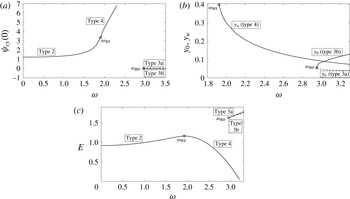
Bifurcation diagrams of solutions of the columnar SLE problem (3.7) with (3.8) for $\unicode[STIX]{x1D70E}=-0.1$ and the range of swirl ratio $0\leqslant \unicode[STIX]{x1D714}\leqslant 3.3$ . (a) $\unicode[STIX]{x1D713}_{cy}(0)$ of the various solution types as a function of $\unicode[STIX]{x1D714}$ ; (b) separation zone sizes $y_{0}$ (for type $3$ solutions) and $y_{w}$ (for type $4$ solutions) as a function of $\unicode[STIX]{x1D714}$ ; (c) $E$ as a function of $\unicode[STIX]{x1D714}$ .

The computed values of the columnar functional $E(\unicode[STIX]{x1D713}_{c};\unicode[STIX]{x1D714};\unicode[STIX]{x1D70E})$ according to (3.9) of the various types of solutions for a diverging pipe with $\unicode[STIX]{x1D70E}=0.2$ are described in figure 2(c). This figure shows that the line of $E(\unicode[STIX]{x1D713}_{c};\unicode[STIX]{x1D714};\unicode[STIX]{x1D70E})$ of decelerated flow states (type $1$ solutions) increases monotonically as $\unicode[STIX]{x1D714}$ increases from $0$ to $\unicode[STIX]{x1D714}_{BD}=1.151$ and is continuously followed by a monotonically increasing line of $E(\unicode[STIX]{x1D713}_{c};\unicode[STIX]{x1D714};\unicode[STIX]{x1D70E})$ of the breakdown states (type $3$ solutions). The lines of $E(\unicode[STIX]{x1D713}_{c};\unicode[STIX]{x1D714};\unicode[STIX]{x1D70E})$ of accelerated flows (type $2$ solutions) and wall-separation states (type $4$ solutions) also increase monotonically with $\unicode[STIX]{x1D714}$ . Similar results are found for other values of diverging pipes with $\unicode[STIX]{x1D70E}>0$ . It is concluded that in the case of a diverging pipe, the type $1$ solutions followed by the type $3$ solutions are global minimum states of $E$ of the columnar SLE problem, the type $4$ solutions are local minimum states of $E$ and the type $2$ solutions (with the highest values of $E$ ) are min–max states of $E$ . According to § 3, only the global and local minimum states of $E$ of the columnar SLE problem represent outlet states of a swirling flow in a long diverging pipe.

Figure 4.

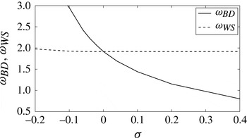
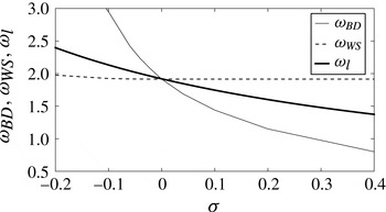
The critical swirls for vortex-breakdown states, $\unicode[STIX]{x1D714}_{BD}$ , and for wall-separation states, $\unicode[STIX]{x1D714}_{WS}$ , as a function of $\unicode[STIX]{x1D70E}$ .

The results of computations for a contracting pipe with $\unicode[STIX]{x1D70E}=-0.1$ in the range $0\leqslant \unicode[STIX]{x1D714}\leqslant 3.5$ are summarized in the bifurcation diagram of solutions of the columnar SLE problem, see figure 3. As before, in figure 3(a), the horizontal axis is the inlet swirl ratio $\unicode[STIX]{x1D714}$ and the vertical axis is the value of the centreline velocity $\unicode[STIX]{x1D713}_{cy}(0)$ of each solution type. It can be seen that only states with accelerated flow along the centreline (type $2$ solutions of the columnar problem; the heavy solid line) exist in the range $0\leqslant \unicode[STIX]{x1D714}<\unicode[STIX]{x1D714}_{WS}$ , where for a contracting pipe with $\unicode[STIX]{x1D70E}=-0.1$ , $\unicode[STIX]{x1D714}_{WS}=1.925$ . The values of $\unicode[STIX]{x1D713}_{cy}(0)$ of these solutions increase above $1$ as $\unicode[STIX]{x1D714}$ is increased toward $\unicode[STIX]{x1D714}_{WS}$ . This branch of solutions is followed by a branch of wall-separation states (type $4$ solutions) with a quasi-stagnation zone in the range $\unicode[STIX]{x1D714}\geqslant \unicode[STIX]{x1D714}_{WS}$ for which $\unicode[STIX]{x1D713}_{cy}(0)$ continues to increase with $\unicode[STIX]{x1D714}$ . Again, the special swirl level $\unicode[STIX]{x1D714}_{WS}$ is the first inlet swirl ratio for the onset of a quasi-stagnation zone near the wall and of wall-separation states (it is marked by a circle in all panels). In addition, the interface position $y_{w}$ of type $4$ solutions decreases from $(1+\unicode[STIX]{x1D70E})^{2}/2=0.405$ as $\unicode[STIX]{x1D714}$ is increased above $\unicode[STIX]{x1D714}_{WS}$ , see figure 3(b). Specifically, the type $4$ solutions are also unique solutions in the range $\unicode[STIX]{x1D714}_{WS}\leqslant \unicode[STIX]{x1D714}\leqslant \unicode[STIX]{x1D714}_{BD}$ , where for $\unicode[STIX]{x1D70E}=-0.1$ , $\unicode[STIX]{x1D714}_{BD}=2.95$ . Additional solutions of breakdown states (of types 3a, the dashed line, and 3b, the solid line) with a centreline stagnation zone appear at swirl ratios above the swirl level $\unicode[STIX]{x1D714}_{BD}$ (see figure 3 a). Again, $\unicode[STIX]{x1D714}_{BD}$ is the first swirl for the onset of breakdown states. The type 3a solutions are characterized by a decreasing size of the stagnation zone $y_{0}$ with increase of $\unicode[STIX]{x1D714}$ above $\unicode[STIX]{x1D714}_{BD}$ while the type 3b solutions have an increasing size of $y_{0}$ (figure 3 b).

We again note that within the range of swirl ratios and pipe contraction parameters studied we did not find additional solutions of the columnar SLE problem (3.7) with (3.8).

The computed values of the columnar functional $E(\unicode[STIX]{x1D713}_{c};\unicode[STIX]{x1D714};\unicode[STIX]{x1D70E})$ for the various types of solutions in a contracting pipe with $\unicode[STIX]{x1D70E}=-0.1$ are described in figure 3(c). This figure shows that the line of $E(\unicode[STIX]{x1D713}_{c};\unicode[STIX]{x1D714};\unicode[STIX]{x1D70E})$ of the accelerated flow states (type $2$ solutions) increases monotonically as $\unicode[STIX]{x1D714}$ increases from $0$ to $\unicode[STIX]{x1D714}_{WS}=1.925$ and is continuously followed by a decreasing line of $E(\unicode[STIX]{x1D713}_{c};\unicode[STIX]{x1D714};\unicode[STIX]{x1D70E})$ of the wall-separation states (type $4$ solutions). The lines of $E(\unicode[STIX]{x1D713}_{c};\unicode[STIX]{x1D714};\unicode[STIX]{x1D70E})$ of the breakdown states (type 3a and type 3b solutions) also increase monotonically with $\unicode[STIX]{x1D714}>2.95$ . Similar results are found for other values of a contracting pipe with $\unicode[STIX]{x1D70E}<0$ . It is concluded that in the case of a contracting pipe, the type $2$ solutions followed by the type $4$ solutions are global minimum states of $E$ , the type 3b solutions are local minimum states of $E$ and the type 3a solutions (with the highest values of $E$ ) are min–max states of $E$ . According to § 3, only the global and local minimum states of $E$ of the columnar SLE problem represent outlet states of a swirling flow in a long contracting pipe.

The above computations demonstrate that for each geometry parameter $\unicode[STIX]{x1D70E}$ there exist two special levels of the incoming flow swirl ratio, one for the first appearance of vortex-breakdown (type 3) states, $\unicode[STIX]{x1D714}_{BD}$ , and the other for the first appearance of wall-separation (type 4) states, $\unicode[STIX]{x1D714}_{WS}$ . These special swirl ratios as a function of $\unicode[STIX]{x1D70E}$ in the range $-0.2\leqslant \unicode[STIX]{x1D70E}\leqslant 0.4$ are shown in figure 4. It is found that for a diverging pipe vortex-breakdown states first appear as swirl is increased from zero. Also, $\unicode[STIX]{x1D714}_{BD}$ decreases significantly with the increase of $\unicode[STIX]{x1D70E}$ while $\unicode[STIX]{x1D714}_{WS}$ stays constant, $\unicode[STIX]{x1D714}_{WS}=1.9159$ . On the other hand, for a contracting pipe, wall-separation states first appear with an increase of $\unicode[STIX]{x1D714}$ from zero. In this case, $\unicode[STIX]{x1D714}_{BD}$ increases significantly with the decrease of $\unicode[STIX]{x1D70E}$ from zero. It shows that, with increase of inlet swirl ratio, decelerated flow and breakdown states dominate flow dynamics in a diverging pipe while accelerated flow and wall-separation states govern flow dynamics in a contracting pipe.

5 Bifurcation diagram of swirling flow states in a pipe

The results from §§ 3 and 4 show that for a long pipe, global and local minimum states of ${\mathcal{E}}(\unicode[STIX]{x1D713}_{s};\unicode[STIX]{x1D714};\unicode[STIX]{x1D70E})$ (solutions of the SLE (PDE) problem (3.4) with (3.5); also steady-state solutions of the unsteady problem (2.1) and (2.2)) are governed by outlet states that are respectively global and local minimum states of $E(\unicode[STIX]{x1D713}_{c};\unicode[STIX]{x1D714};\unicode[STIX]{x1D70E})$ ) (solutions of the columnar SLE problem). We emphasize again that min–max states of $E(\unicode[STIX]{x1D713}_{c};\unicode[STIX]{x1D714};\unicode[STIX]{x1D70E})$ ) (of the columnar SLE problem) are not outlet profiles of min–max states of ${\mathcal{E}}(\unicode[STIX]{x1D713}_{s};\unicode[STIX]{x1D714};\unicode[STIX]{x1D70E})$ . Therefore, in a diverging pipe with $\unicode[STIX]{x1D70E}>0$ , type $1$ decelerated flow states turning into type $3$ breakdown states are global minimum states of ${\mathcal{E}}(\unicode[STIX]{x1D713}_{s};\unicode[STIX]{x1D714};\unicode[STIX]{x1D70E})$ and type $4$ wall-separation states are local minimum states of ${\mathcal{E}}(\unicode[STIX]{x1D713}_{s};\unicode[STIX]{x1D714};\unicode[STIX]{x1D70E})$ . Following an analysis similar to that in Wang & Rusak (Reference Wang and Rusak1997a ), it can be shown that type $2$ accelerated flow states must exist between the global and local minimum states and are min–max states of ${\mathcal{E}}(\unicode[STIX]{x1D713}_{s};\unicode[STIX]{x1D714};\unicode[STIX]{x1D70E})$ . On the other hand, for a contracting pipe with $\unicode[STIX]{x1D70E}<0$ , type $2$ accelerated flow states turning into type $4$ wall-separation states are global minimum states of ${\mathcal{E}}(\unicode[STIX]{x1D713}_{s};\unicode[STIX]{x1D714};\unicode[STIX]{x1D70E})$ and type 3b breakdown states are local minimum states of ${\mathcal{E}}(\unicode[STIX]{x1D713}_{s};\unicode[STIX]{x1D714};\unicode[STIX]{x1D70E})$ . Again, it can be shown that type 3a breakdown states are min–max states of ${\mathcal{E}}(\unicode[STIX]{x1D713}_{s};\unicode[STIX]{x1D714};\unicode[STIX]{x1D70E})$ between the type $4$ and type 3b states.

We want to clarify that within the range of swirl levels and pipe parameters studied in the following discussion, the present solutions of the SLE (PDE) problem and the unsteady numerical simulations do not show any additional steady flow states. The flow always converged in time to either the centreline decelerated flow, accelerated flow, breakdown or the wall-separation states. Following Rusak & Wang (Reference Rusak and Wang2014), additional higher-order solutions may exist at inlet swirl levels beyond the range of values studied in this paper. These states must be additional min–max states of ${\mathcal{E}}(\unicode[STIX]{x1D713}_{s};\unicode[STIX]{x1D714};\unicode[STIX]{x1D70E})$ .

In addition, the inviscid-limit flow linear stability studies in Wang & Rusak (Reference Wang and Rusak1996) and in Rusak & Judd (Reference Rusak and Judd2001) and the inviscid-limit flow simulations of Rusak et al. (Reference Rusak, Wang, Xu and Taylor2012) and of Rusak & Wang (Reference Rusak and Wang2014) demonstrate that the global and local minimum solutions of ${\mathcal{E}}$ according to the SLE (PDE) problem are linearly stable to either infinitesimal or finite-amplitude perturbations of a given mode form. On the other hand, the min–max solutions of ${\mathcal{E}}$ of the SLE (PDE) problem are unstable. Within the range of inlet swirl levels studied in this paper, the present unsteady simulations also support this fundamental relationship between the linear stability analysis and energy stability.

The SLE (PDE) problem (3.4) with (3.5) is solved for various $\unicode[STIX]{x1D70E}$ and $\unicode[STIX]{x1D714}$ using the numerical method described in appendix B. Two pipe geometry profiles are used in these computations, $R(x)=1+(\unicode[STIX]{x1D70E}/2)[1+\sin (\unicode[STIX]{x03C0}(x/L-1/2))]$ and $R(x)=1+(\unicode[STIX]{x1D70E}/2)[1+\tanh (10(x-1))]$ for $0\leqslant x\leqslant L$ , both with $L=6$ . For a given geometry parameter $\unicode[STIX]{x1D70E}$ , a steady-state solution $\unicode[STIX]{x1D713}_{s}(x,y)$ has been first established at $\unicode[STIX]{x1D714}=0$ , and then, through a successive increase of $\unicode[STIX]{x1D714}$ in small steps, steady-state solutions $\unicode[STIX]{x1D713}_{s}(x,y)$ are found at higher values of $\unicode[STIX]{x1D714}$ . In this way, for a diverging pipe with $\unicode[STIX]{x1D70E}>0$ , branches of type $1$ solutions (decelerated flow along the centreline) followed by type $3$ solutions (vortex-breakdown states) of the SLE (PDE) problem have been established. For a contracting pipe with $\unicode[STIX]{x1D70E}<0$ , branches of type $2$ solutions (accelerated flow along the centreline) followed by type $4$ solutions (wall-separation states) of the SLE (PDE) problem have also been found. In addition, in order to determine solutions of type $2$ and $4$ when $\unicode[STIX]{x1D70E}>0$ , a type $4$ solution of the problem with $\unicode[STIX]{x1D70E}=0$ at $\unicode[STIX]{x1D714}$ that is slightly greater than $\unicode[STIX]{x1D714}_{WS}$ (according to figure 4) has been formed. Through a successive increase of $\unicode[STIX]{x1D70E}$ in small steps, type $4$ solutions are found at a desired value of $\unicode[STIX]{x1D70E}>0$ . Then, by successively increasing $\unicode[STIX]{x1D714}$ in small steps, the branch of type $4$ solutions is established. By decreasing $\unicode[STIX]{x1D714}$ in small steps down to $\unicode[STIX]{x1D714}_{WS}$ , the first type $2$ solution is found and forms a fold point. This solution is used to establish the branch of type $2$ solutions for $\unicode[STIX]{x1D714}>\unicode[STIX]{x1D714}_{WS}$ . Similarly, in order to determine solutions of types $1$ and $3$ when $\unicode[STIX]{x1D70E}<0$ , a type $3$ solution of the problem with $\unicode[STIX]{x1D70E}=0$ and $\unicode[STIX]{x1D714}$ slightly greater than $\unicode[STIX]{x1D714}_{BD}(\unicode[STIX]{x1D70E}=0)$ (according to figure 4) has been formed, and through a successive increase of $\unicode[STIX]{x1D70E}$ in small steps, type $3$ solutions are found at a desired value of $\unicode[STIX]{x1D70E}<0$ . Then, by decreasing $\unicode[STIX]{x1D714}$ in small steps, the branches of type 3a and 3b solutions are found, with a fold point at $\unicode[STIX]{x1D714}_{BD}$ . For both pipe geometries used in the computations and for the range of inlet swirl studied, we found almost same outlet profiles (within three digits accuracy) of the computed streamfunction and of the axial velocity for all type of solutions. This indicates that when the pipe is sufficiently long the details of the pipe monotonic geometry do not affect the outlet state.

Moreover, the unsteady flow problem (2.1) and (2.2) with the assumed boundary conditions is solved for various $\unicode[STIX]{x1D70E}$ and $\unicode[STIX]{x1D714}$ using the numerical time integration scheme described in appendix A. In all simulations studied we used only one pipe geometry, $R(x)=1+(\unicode[STIX]{x1D70E}/2)[1+\sin (\unicode[STIX]{x03C0}(x/L-1/2))]$ with $L=6$ . For a given $\unicode[STIX]{x1D70E}$ , starting from an initial columnar state at $\unicode[STIX]{x1D714}=0.2$ , flow dynamics converges after long time to a time-asymptotic state $\unicode[STIX]{x1D713}(x,y,t\gg 1)$ that is nearly the steady state at the given $\unicode[STIX]{x1D70E}$ and $\unicode[STIX]{x1D714}=0.2$ . Then, through successively using the time-asymptotic state of a previous $\unicode[STIX]{x1D714}$ as an initial state and increasing $\unicode[STIX]{x1D714}$ in small steps, branches of time-asymptotic states $\unicode[STIX]{x1D713}(x,y,t\gg 1)$ of the unsteady problem (2.1) and (2.2) have been established. In this way, when $\unicode[STIX]{x1D70E}>0$ , branches of type $1$ time-asymptotic states (decelerated flow along the centreline) followed by type $3$ time-asymptotic states (vortex-breakdown states) are found. When $\unicode[STIX]{x1D70E}<0$ , branches of type $2$ time-asymptotic states (accelerated flow along the centreline) followed by type $4$ time-asymptotic states (wall-separation states) are formed. In addition, when $\unicode[STIX]{x1D70E}>0$ , type $4$ time-asymptotic states are found by initially perturbing a columnar state at $\unicode[STIX]{x1D70E}=0$ and $\unicode[STIX]{x1D714}>\unicode[STIX]{x1D714}_{WS}(\unicode[STIX]{x1D70E}=0)$ and computing flow dynamics until a type $4$ time-asymptotic state is established. Using this state as an initial state and successively increasing $\unicode[STIX]{x1D70E}$ in small steps and in time to a desired $\unicode[STIX]{x1D70E}>0$ , a type $4$ time-asymptotic state is found. Then, by increasing or decreasing $\unicode[STIX]{x1D714}$ in small steps, the branch of type $4$ time-asymptotic states is established.

We note that in the simulations no time-asymptotic states of type $2$ are found when $\unicode[STIX]{x1D70E}>0$ and no type $1$ and 3a states are found when $\unicode[STIX]{x1D70E}<0$ . This demonstrates that these states are indeed unstable, as has been mentioned above, and cannot be formed as part of time-asymptotic flow evolution. We also note that for all $\unicode[STIX]{x1D70E}$ the vortex-breakdown stagnation zones as well as the wall-separation quasi-stagnation zones appear naturally during the computed flow evolution to time-asymptotic states, with no special assumption in the simulation procedure. Specifically, no averaging step of computations is needed during the simulation of flow evolution, in contrast the inviscid-limit flow simulations of Rusak et al. (Reference Rusak, Wang, Xu and Taylor2012) that studied the dynamics of Lamb–Oseen vortices with small vortex cores.

6 Uniqueness of steady flow state when $0\leqslant \unicode[STIX]{x1D714}<\unicode[STIX]{x1D714}_{l}(D)$

The results of § 5 demonstrate that the unsteady flow problem (2.1)–(2.2) with the assumed boundary conditions has a unique steady-state solution in the range of incoming swirl ratio $0\leqslant \unicode[STIX]{x1D714}<\unicode[STIX]{x1D714}_{WS}$ when $\unicode[STIX]{x1D70E}>0$ and in the range $0\leqslant \unicode[STIX]{x1D714}<\unicode[STIX]{x1D714}_{BD}$ when $\unicode[STIX]{x1D70E}<0$ (see figure 4).

In this section we prove the uniqueness of the steady-state flow problem described by the SLE (PDE) (3.4) and boundary conditions (3.5) in a definite range of the incoming swirl ratios $0\leqslant \unicode[STIX]{x1D714}<\unicode[STIX]{x1D714}_{l}(D)$ . Here $D$ is the flow domain, $D\equiv \{(x,y)\in \mathbb{R}^{2}~|~0\leqslant x\leqslant L,~0\leqslant y\leqslant R^{2}(x)/2\}$ . Assuming $\unicode[STIX]{x1D713}_{s}(x,y)$ is a solution of (3.4) and (3.5), a perturbed solution is given by $\unicode[STIX]{x1D713}_{s}^{\ast }(x,y)=\unicode[STIX]{x1D713}_{s}(x,y)+\overline{\unicode[STIX]{x1D713}}(x,y)$ where the perturbation streamfunction $\overline{\unicode[STIX]{x1D713}}(x,y)$ and related $\unicode[STIX]{x1D714}_{l}(D)$ are found from solving the following eigenvalue problem:

in the domain $D$ with the homogeneous boundary conditions:

The incoming limit swirl level $\unicode[STIX]{x1D714}_{l}(D)$ is defined as the first eigenvalue of the linearized SLE problem (6.1) and (6.2). In the following discussion, we show that when $0\leqslant \unicode[STIX]{x1D714}<\unicode[STIX]{x1D714}_{l}(D)$ the only solution of this problem is the trivial solution, $\overline{\unicode[STIX]{x1D713}}=0$ , and then the solution $\unicode[STIX]{x1D713}_{s}(x,y)$ is unique.

The eigenvalues $\unicode[STIX]{x1D714}_{l}(D)$ of a swirling flow in a pipe where $R(x)=1+(\unicode[STIX]{x1D70E}/2)[1+\tanh (10(x-1))]$ and in a pipe where $R(x)=1+(\unicode[STIX]{x1D70E}/2)[1+\sin (\unicode[STIX]{x03C0}(x/L-1/2))]$ , for $0\leqslant x\leqslant L$ , both with $L=6$ and with various values of $\unicode[STIX]{x1D70E}$ , were computed numerically using a standard eigenvalue solver of (6.1) and (6.2). The resulting values of $\unicode[STIX]{x1D714}_{l}(D)$ as a function of $\unicode[STIX]{x1D70E}$ in the range $-0.2\leqslant \unicode[STIX]{x1D70E}\leqslant 0.4$ are numerically nearly the same for both pipe geometries (within 3 digits) and are presented in figure 11 (the solid heavy line). Also shown for comparison are the curves of $\unicode[STIX]{x1D714}_{BD}$ (the thin line) and $\unicode[STIX]{x1D714}_{WS}$ (the dash line) as function of $\unicode[STIX]{x1D70E}$ . We find that $\unicode[STIX]{x1D714}_{l}(D)=\unicode[STIX]{x1D714}_{BD}=\unicode[STIX]{x1D714}_{WS}=1.92$ when $\unicode[STIX]{x1D70E}=0$ (the case of a straight pipe, Rusak & Wang Reference Rusak and Wang2014). The swirl level $\unicode[STIX]{x1D714}_{l}(D)$ decreases with the increase of pipe divergence (when $\unicode[STIX]{x1D70E}>0$ ) and increases with increase of size of the pipe contraction (when $\unicode[STIX]{x1D70E}<0$ ). Also, $\unicode[STIX]{x1D714}_{BD}<\unicode[STIX]{x1D714}_{l}(D)<\unicode[STIX]{x1D714}_{WS}$ when $\unicode[STIX]{x1D70E}>0$ and $\unicode[STIX]{x1D714}_{WS}<\unicode[STIX]{x1D714}_{l}(D)<\unicode[STIX]{x1D714}_{BD}$ when $\unicode[STIX]{x1D70E}<0$ .

Figure 11.

The critical swirl level $\unicode[STIX]{x1D714}_{l}(D)$ (the heavy line) as a function of $\unicode[STIX]{x1D70E}$ for a pipe with $R(x)=1+(\unicode[STIX]{x1D70E}/2)[1+\tanh (10(x-1))]$ and for a pipe with $R(x)=1+(\unicode[STIX]{x1D70E}/2)[1+\sin (\unicode[STIX]{x03C0}(x/L-1/2))]$ with $L=6$ . Also shown are the swirl levels for vortex-breakdown states, $\unicode[STIX]{x1D714}_{BD}$ (the thin line), and for wall-separation states, $\unicode[STIX]{x1D714}_{WS}$ (the dash-dot line), as a function of $\unicode[STIX]{x1D70E}$ .

We prove now that there exists a unique weak solution of the SLE (PDE) problem (3.4) and (3.5) in the domain $D$ and with the definitions (3.2) and (3.3) when $0\leqslant \unicode[STIX]{x1D714}<\unicode[STIX]{x1D714}_{l}(D)$ . Following Rusak & Wang (Reference Rusak and Wang2014), the swirl level $\unicode[STIX]{x1D714}_{l}(D)$ can also be determined by the Rayleigh quotient

Note that this is a weighted Poincaré inequality, where the minimization process is taken over all the test functions $\overline{\unicode[STIX]{x1D713}}$ that are admissible with the boundary conditions (3.5). Also, one may replace $D$ in (6.3) by any other bounded subdomain $\overline{D}$ , $\overline{D}\subset D$ , with piecewise-smooth boundaries and choosing $\overline{\unicode[STIX]{x1D713}}=0$ in the domain $D-\overline{D}$ . It can be shown that if $\overline{D}$ and $D$ are bounded domains with piecewise-smooth boundaries then $\unicode[STIX]{x1D714}_{l}(\overline{D})\geqslant \unicode[STIX]{x1D714}_{l}(D)$ . This is demonstrated in figure 11 where $\unicode[STIX]{x1D714}_{l}$ decreases with increase of $\unicode[STIX]{x1D70E}$ from negative to positive values.

In addition, the energy functional associated with the SLE (PDE) (3.4) is given from (3.6) for the case of a solid-body rotation by:

Based on (6.3), a global minimum state of the functional (6.4) exists by using a standard compactness argument, see for example Wang & Rusak (Reference Wang and Rusak1997a ). We denote this global minimum state by $\unicode[STIX]{x1D713}_{g}$ . Note that we enforce $0\leqslant \unicode[STIX]{x1D713}_{g}\leqslant 1/2$ for correctly describing solutions with stagnation or quasi-stagnation zones; see Rusak & Wang (Reference Rusak and Wang2014).

For each function $0\leqslant \unicode[STIX]{x1D713}_{s}(x,y)\leqslant 1/2$ in $D$ , we partition the domain $D$ into three sets, $D_{\unicode[STIX]{x1D713}_{s}}^{+}\equiv \{(x,y)\in D\text{ and }0<\unicode[STIX]{x1D713}_{s}(x,y)<1/2\}$ , $D_{\unicode[STIX]{x1D713}_{s}}^{0}\equiv \{(x,y)\in D\text{ and }\unicode[STIX]{x1D713}_{s}(x,y)=0\}$ and $D_{\unicode[STIX]{x1D713}_{s}}^{1/2}\equiv \{(x,y)\in D\text{ and }\unicode[STIX]{x1D713}_{s}(x,y)=1/2\}$ . Here, $D_{\unicode[STIX]{x1D713}_{s}}^{0}$ and $D_{\unicode[STIX]{x1D713}_{s}}^{1/2}$ represent the zones of breakdown and wall separation of $\unicode[STIX]{x1D713}_{s}$ , respectively. For a state without any separation zone, $D=D_{\unicode[STIX]{x1D713}_{s}}^{+}$ . For a state with only a breakdown zone, $D=D_{\unicode[STIX]{x1D713}_{s}}^{+}\cup D_{\unicode[STIX]{x1D713}_{s}}^{0}$ and $D_{\unicode[STIX]{x1D713}_{s}}^{1/2}=0$ , while for a state with only a wall-separation zone, $D=D_{\unicode[STIX]{x1D713}_{s}}^{+}\cup D_{\unicode[STIX]{x1D713}_{s}}^{1/2}$ and $D_{\unicode[STIX]{x1D713}_{s}}^{0}=0$ . In general, for a state with both separation zones, $D=D_{\unicode[STIX]{x1D713}_{s}}^{+}\cup D_{\unicode[STIX]{x1D713}_{s}}^{0}\cup D_{\unicode[STIX]{x1D713}_{s}}^{1/2}$ .

The first variation of (6.4) is given by:

Here, the perturbation test function $(\overline{\unicode[STIX]{x1D713}})^{+}$ is defined by:

Note that $(-\overline{\unicode[STIX]{x1D713}})^{+}=0$ if $\overline{\unicode[STIX]{x1D713}}\geqslant 0$ and $(-\overline{\unicode[STIX]{x1D713}})^{+}=-\overline{\unicode[STIX]{x1D713}}$ if $\overline{\unicode[STIX]{x1D713}}<0$ . The relationship $\langle \unicode[STIX]{x1D6FF}{\mathcal{E}}(\unicode[STIX]{x1D713}_{s};\unicode[STIX]{x1D714};\unicode[STIX]{x1D70E}),\overline{\unicode[STIX]{x1D713}}\rangle \geqslant 0$ for all test functions $\overline{\unicode[STIX]{x1D713}}$ is a definition of a solution in the weak sense. In this way, this solution is extended to include solutions with either a stagnation or a quasi-stagnation zone (Rusak & Wang Reference Rusak and Wang2014).

For each test function $\overline{\unicode[STIX]{x1D713}}$ that is compactly supported on $D_{\unicode[STIX]{x1D713}_{g}}^{+}$ , we find in the domain $D$ that the global minimum state $\unicode[STIX]{x1D713}_{g}$ satisfies $\langle \unicode[STIX]{x1D6FF}{\mathcal{E}}(\unicode[STIX]{x1D713}_{g};\unicode[STIX]{x1D714};\unicode[STIX]{x1D70E}),\overline{\unicode[STIX]{x1D713}}\rangle =0$ , or from (6.5):

Let $\hat{\unicode[STIX]{x1D713}}$ be a test function that is compactly supported on $D_{\unicode[STIX]{x1D713}_{g}}^{+}$ . Assuming $\unicode[STIX]{x1D713}_{s}=\unicode[STIX]{x1D713}_{g}+\hat{\unicode[STIX]{x1D713}}$ is another weak solution of the problem, we also have from (6.5):

Also, we find in the domain $D$ the following two relationships:

From (6.9a ) and (6.9b ) we have

Substituting (6.10) into (6.8), replacing $\unicode[STIX]{x1D713}_{s}=\unicode[STIX]{x1D713}_{g}+\hat{\unicode[STIX]{x1D713}}$ and using (6.7) for $\unicode[STIX]{x1D713}_{g}$ we obtain

We note that since $\unicode[STIX]{x1D713}_{s}(x,y)=0$ on $D_{\unicode[STIX]{x1D713}_{s}}^{0}$ we have $\hat{\unicode[STIX]{x1D713}}=-\unicode[STIX]{x1D713}_{g}$ on $D_{\unicode[STIX]{x1D713}_{s}}^{0}$ . Similarly, since $\unicode[STIX]{x1D713}_{s}(x,y)=1/2$ on $D_{\unicode[STIX]{x1D713}_{s}}^{1/2}$ we have $\hat{\unicode[STIX]{x1D713}}=(1/2-\unicode[STIX]{x1D713}_{g})$ on $D_{\unicode[STIX]{x1D713}_{s}}^{1/2}$ . Let us now choose the specific case where $\overline{\unicode[STIX]{x1D713}}=-\hat{\unicode[STIX]{x1D713}}$ . Using the fact that $0\leqslant \unicode[STIX]{x1D713}_{g}\leqslant 1/2$ , we have $\overline{\unicode[STIX]{x1D713}}=-\hat{\unicode[STIX]{x1D713}}=\unicode[STIX]{x1D713}_{g}\geqslant 0~\text{on}~D_{\unicode[STIX]{x1D713}_{s}}^{0}$ and $\overline{\unicode[STIX]{x1D713}}=-\hat{\unicode[STIX]{x1D713}}=-(1/2-\unicode[STIX]{x1D713}_{g})\leqslant 0~\text{on}~D_{\unicode[STIX]{x1D713}_{s}}^{1/2}$ . Therefore, from the definitions of $(\overline{\unicode[STIX]{x1D713}})^{+}$ and $(-\overline{\unicode[STIX]{x1D713}})^{+}$ , the last two terms of (6.11) vanish. Substituting this into (6.11) and using the fact that $\hat{\unicode[STIX]{x1D713}}$ is compactly supported on $D_{\unicode[STIX]{x1D713}_{g}}^{+}$ , we find that $\hat{\unicode[STIX]{x1D713}}=0$ in $D_{\unicode[STIX]{x1D713}_{g}}^{0}\cup D_{\unicode[STIX]{x1D713}_{g}}^{1/2}$ and, therefore, the first variation of ${\mathcal{E}}$ satisfies

Since $D_{\unicode[STIX]{x1D713}_{g}}^{+}\subset D$ , we have $\unicode[STIX]{x1D714}_{l}(D_{\unicode[STIX]{x1D713}_{g}}^{+})\geqslant \unicode[STIX]{x1D714}_{l}(D)$ . Since $0\leqslant \unicode[STIX]{x1D714}<\unicode[STIX]{x1D714}_{l}(D)$ , according to (6.3), (6.12) is possible only if $\hat{\unicode[STIX]{x1D713}}=0$ and thus $\unicode[STIX]{x1D713}_{s}|_{D_{\unicode[STIX]{x1D713}_{g}}^{+}}=\unicode[STIX]{x1D713}_{g}|_{D_{\unicode[STIX]{x1D713}_{g}}^{+}}$ , which implies that $D_{\unicode[STIX]{x1D713}_{g}}^{+}\subset D_{\unicode[STIX]{x1D713}_{s}}^{+}$ . Similarly, by swapping $\unicode[STIX]{x1D713}_{s}$ and $\unicode[STIX]{x1D713}_{g}$ in above argument we can show that $\unicode[STIX]{x1D713}_{g}|_{D_{\unicode[STIX]{x1D713}_{s}}^{+}}=\unicode[STIX]{x1D713}_{s}|_{D_{\unicode[STIX]{x1D713}_{s}}^{+}}$ , which implies that $D_{\unicode[STIX]{x1D713}_{s}}^{+}\subset D_{\unicode[STIX]{x1D713}_{g}}^{+}$ . Hence we have $D^{+}\equiv D_{\unicode[STIX]{x1D713}_{g}}^{+}=D_{\unicode[STIX]{x1D713}_{s}}^{+}$ and $\unicode[STIX]{x1D713}_{g}|_{D^{+}}=\unicode[STIX]{x1D713}_{s}|_{D^{+}}$ . Moreover, since $\unicode[STIX]{x1D713}_{g}(x,y)\in \{0,1/2\},~\unicode[STIX]{x1D713}_{s}(x,y)\in \{0,1/2\}$ for each $(x,y)\in D-D^{+}$ , and since $\unicode[STIX]{x1D713}_{g}$ and $\unicode[STIX]{x1D713}_{s}$ are continuous on $D$ , we conclude that $\unicode[STIX]{x1D713}_{s}=\unicode[STIX]{x1D713}_{g}$ . Therefore, the global minimum state of ${\mathcal{E}}$ is a unique solution on $D$ when $0\leqslant \unicode[STIX]{x1D714}<\unicode[STIX]{x1D714}_{l}(D)$ .

We provide physical meaning to the above uniqueness proof. The original SLE (PDE) problem (3.4) and (3.5) is linear for as long as there is no separation zone in the flow, but it becomes nonlinear with the appearance of vortex-breakdown or wall-separation zones where conditions (3.2) and (3.3) are applied. The uniqueness of the computed states is related to the linear eigenvalue problem (6.1) and (6.2) and its first eigenvalue given by (6.3). This problem (6.1) is a linearization of (3.4) and (3.5) with respect to a steady perturbation about the steady-state solution. Yet, the proof is given even for cases where the global minimum state of ${\mathcal{E}}$ describes states with breakdown or wall-separation zones and the SLE (PDE) problem is nonlinear. The eigenvalue (6.3) provides a limit swirl level below which the columnar SLE computations, the SLE (PDE) computations and the unsteady simulations must show only one solution, no matter what the type is, whether decelerated flow state, accelerated flow state, breakdown state or wall-separation state. Indeed, the results in figure 11 show this important point. Although not proven analytically, the unsteady simulations also demonstrate that in the range of unique states the steady-state flow is asymptotically stable. This highlights the correlation between the uniqueness of a global minimum state and its stability even under the nonlinear situations.