1 Introduction
Despite receiving the attention of many researchers, turbulent flows still challenge the scientific community in many aspects. One of the main open issues in this topic is the instability problem, which triggers turbulent motion from a laminar regime (Eckert Reference Eckert2010; Sano & Tamai Reference Sano and Tamai2016). The transition from laminar to turbulent flow exhibits a diversity of states that are characterised by a combination of these two extreme poles. The interpretation of the flow as a bistable reaction–diffusion system with an advection propagation front (Barkley et al. Reference Barkley, Song, Mukund, Lemoult, Avila and Hof2015; Graham Reference Graham2015) provides useful insights for the analysis and the construction of simplified models of turbulence growth. Some important recent works have been dedicated to the investigation of how, and in which conditions, patches of turbulent flow surrounded by the laminar regime propagate throughout the domain in some cases, while they die in others (Barkley et al. Reference Barkley, Song, Mukund, Lemoult, Avila and Hof2015). The competition between laminar and turbulent regimes inside the transitional flow has been described not only by the Navier–Stokes equations but also by other dynamical equations, which were conceived to mimic turbulent features and were inspired by models for the description of phase transition (Pomeau Reference Pomeau2015). As we will show here, the pronounced intermittent flow that emerges from this competition between laminar and turbulent parts can be observed not only in transitional Newtonian regimes but also in non-Newtonian turbulent regimes, such as polymer drag-reducing flows.
We can take the discussion conducted by Barkley (Reference Barkley2016) with respect to the Newtonian turbulence in a pipe as the starting point for understanding transition features. Barkley (Reference Barkley2016) described in detail how models that focus on the turbulence intensity as the main variable can capture the essential characteristics of the transition phenomenon. The basic ideas of turbulent transition can be gradually recognised by starting from defining potential functions, evolving to the analogy with phase transition, and finally constructing an analogy with the passage of signals in a neuron. It is worth noting that these models predict an important experimental result that is very relevant to the present work – namely, the existence of a first and a second critical Reynolds number (which are explained next). The first is a Reynolds-number value below which the flow has only the laminar linearly stable solution and above which a two-branched bifurcation associated with two turbulent solutions begin to coexist with the laminar flow. While the upper-branch turbulent solution is linearly stable, the lower branch is an unstable turbulent solution. The second critical Reynolds number delimits an interchange between the laminar and the upper-branch turbulent solution with respect to their stability status (as explained next). Inspired by the analogy with phase transition, Pomeau (Reference Pomeau1986, Reference Pomeau2015) employed the expressions ‘metastable’ and (strictly) ‘stable’ to indicate the growth direction of the two-phase system. The strictly stable phase advances towards the metastable phase. The analogy with potentials illustrates the subject by considering that the metastable solution has a shallower valley than the strictly stable solution. Below the second critical value of the Reynolds number,
 $Re_{b,c}$
, the laminar solution is strictly stable while the turbulent solution is metastable. Above
 $Re_{b,c}$
, they invert and the turbulent solution becomes strictly stable, while the laminar solution becomes metastable. This interchange establishes the existence of two subregimes inside the transition regime.
Nonlinear travelling wave solutions to the Navier–Stokes equations have been identified in planar Poiseuille flows (as also in Couette flows), which are generally called exact coherent structures (see Waleffe Reference Waleffe2001), and which are in direct connection with the picture that was outlined previously. These solutions also come in pairs – upper (farther from the laminar) and lower (closer to the laminar) branches – after a threshold point of bifurcation, and they do not present the complex erratic spatio-temporal dynamics that are typical of turbulent flows. The recent studies of these solutions and their instabilities provide a new understanding of transitional flows.
Drag-reducing viscoelastic turbulent flows have been known since the work of Toms (Reference Toms1948), when it was found that the addition of a small amount of polymers into a turbulent Newtonian flow can induce drag reduction (DR). The understanding of the interaction process between polymers and turbulence to explain how DR occurs has received relevant contributions (Min, Yoo & Choi Reference Min, Yoo and Choi2003a
; Min et al.
Reference Min, Yoo, Choi and Joseph2003b
; Dubief et al.
Reference Dubief, White, Terrapon, Shaqfeh, Moin and Lele2004; Kim et al.
Reference Kim, Li, Sureshkumar, Balachandar and Adrian2007) but many aspects still deserve more investigations (Thais, Gatski & Mompean Reference Thais, Gatski and Mompean2012, Reference Thais, Gatski and Mompean2013a
,Reference Thais, Gatski and Mompean
b
; Graham Reference Graham2014; Pereira Reference Pereira2016; Pereira et al.
Reference Pereira, Mompean, Thais and Soares2017a
,Reference Pereira, Mompean, Thais, Soares and Thompson
b
,Reference Pereira, Mompean, Thais and Thompson
c
,Reference Pereira, Mompean, Thompson and Soares
d
; Pereira, Mompean & Soares Reference Pereira, Mompean and Soares2018), and we can consider that this subject is another open issue in turbulence. Probably the most important result obtained so far is the existence of a limiting situation where DR is saturated, i.e. it would not be enhanced by adding more polymers or increasing their molecular weight. This subregime is called maximum drag reduction (MDR) (or Virk’s asymptotic limit), and was discovered by Virk and co-workers (Virk, Mickley & Smith Reference Virk, Mickley and Smith1967, Reference Virk, Mickley and Smith1970; Virk Reference Virk1975a
,Reference Virk
b
) in experimental investigations. Another important finding concerning viscoelastic turbulent flows is the existence of two other subregimes of DR – namely low drag reduction (LDR) and high drag reduction (HDR) – the latter being upper-bounded by the MDR (Warholic, Massah & Hanratty Reference Warholic, Massah and Hanratty1999). It is generally accepted that this regime change occurs at
 $\text{DR}\approx 40\,\%$
(White & Mungal Reference White and Mungal2008). Roughly, the LDR regime is characterised by statistics that are more similar to those found in Newtonian turbulence, while the HDR regime presents statistics that are more similar to the MDR.
Recently, important contributions to the understanding of these three manifestations of DR were given by Xi & Graham (Reference Xi and Graham2010), who indicated that, during both the HDR and the MDR subregimes, viscoelastic turbulent flows fluctuate between two distinct states: active and hibernating. The former is related to the basic dynamical elements of Newtonian near-wall turbulence, exhibiting a higher drag. In contrast, the turbulent structures almost vanish during the latter state, which reduces the drag. In the particular MDR subregime, the time-average velocity profile that emerges from this intermittent behaviour is given by the Virk’s asymptote. Xi & Graham (Reference Xi and Graham2010) offer an explanation for the oscillations between active and hibernating turbulence in the viscoelastic context as a result of the following cycling mechanism. When coiled polymers are exposed to an active state, turbulence acts to stretch these polymers (see also Graham Reference Graham2014). This process increases the stresses associated with the fluid, which in turn diminishes turbulence activity, eventually leading the flow to a hibernating state. In this state, turbulence does not induce the stretching of polymers, which tend to coil, and consequently decreases the stresses that were acting to suppress turbulence. This condition leads to an active turbulent state again, restarting the cycle.
Despite the absence of a definitive consensus concerning the physical mechanisms that drive each of the DR scenarios presented above, many of the features of viscoelastic turbulence – including the MDR subregime, as well as the LDR and HDR subregimes – were obtained not only experimentally but also numerically using direct numerical simulations (DNS) and employing the finitely extensible nonlinear elastic model with the Peterlin approximation (FENE-P fluids), following the seminal work of Sureshkumar, Beris & Handler (Reference Sureshkumar, Beris and Handler1997). This fact has given a significant credit to this approach, despite the fact that the FENE-P model is a crude approximation for the real behaviour of polymer molecules. In addition, in a numerical work, it is easier to explore the DR space while controlling both the Reynolds number (the ratio of inertial to viscous effects) and the Weissenberg number (the ratio of elastic to viscous effects).
The discovery of elastic turbulence (Vinogradov & Mannin Reference Vinogradov and Mannin1965) and the recent studies on elasto-inertial turbulence (EIT) (Dubief, Terrapon & Soria Reference Dubief, Terrapon and Soria2013; Choueiri, Lopez & Hof Reference Choueiri, Lopez and Hof2018; Sid, Terrapon & Dubief Reference Sid, Terrapon and Dubief2018; Shekar et al. Reference Shekar, McMullen, Wang, McKeon and Graham2019) have shown that elastic effects produced by the interactions between the flow and the polymer can have a fundamental influence on the origin of turbulence of viscoelastic fluids. The addition of polymers for high Reynolds numbers induces DR. On the other hand, for low values of Reynolds number, elasticity can trigger turbulence before reaching the Newtonian critical threshold, the so-called ‘early turbulence’ (see Hansen & Little Reference Hansen and Little1974). Recent experimental results provided by Choueiri et al. (Reference Choueiri, Lopez and Hof2018) and corroborated by the numerical investigation of Shekar et al. (Reference Shekar, McMullen, Wang, McKeon and Graham2019) suggest that the laminar flow can be achieved with the addition of polymers (or increasing the Weissenberg number), but after a subsequent concentration increase, the flow acquires a non-laminar character. The EIT was shown to be associated with two-dimensional elasto-inertial instabilities (Sid et al. Reference Sid, Terrapon and Dubief2018), and the sheet-like structures found in EIT due to strong localised (polymer) stress fluctuations are similar to those present in Tollmien–Schlichting waves found in Newtonian flows (Shekar et al. Reference Shekar, McMullen, Wang, McKeon and Graham2019).
A number of numerical works have found topological and dynamical modifications where elasticity is increased when starting from a Newtonian turbulent flow, as in Dubief et al. (Reference Dubief, White, Terrapon, Shaqfeh, Moin and Lele2004, Reference Dubief, Terrapon, White, Shaqfeh, Moin and Lele2005, Reference Dubief, White, Shaqfeh and Terrapon2011, Reference Dubief, Terrapon and Soria2013), Xi & Graham (Reference Xi and Graham2010, Reference Xi and Graham2012) and Pereira et al. (Reference Pereira, Mompean, Thais and Thompson2017c
). These studies suggest several common aspects between the viscoelastic drag-reducing turbulence and the Newtonian transition to turbulence. In particular, Dubief et al. (Reference Dubief, White, Shaqfeh and Terrapon2011) have demonstrated that MDR is a unique transitional state between laminar and turbulent flow and, as such, can be found in Newtonian transitional flows, i.e. are not restricted to viscoelastic drag-reducing turbulent flows. These similarities are explored in the present work by employing DNS in a plane Poiseuille flow. Hence, we take into account incompressible flows induced by a pressure gradient between two stationary parallel plates. Inertial effects are related to the Reynolds number
 $Re_{b}=hU_{b}/\unicode[STIX]{x1D708}_{tot}$
(where
 $h$
denotes the plane Poiseuille half-width,
 $U_{b}$
is the bulk velocity and
 $\unicode[STIX]{x1D708}_{tot}$
represents the solution viscosity), while elastic effects are linked with the Weissenberg number
 $Wi_{b}=\unicode[STIX]{x1D706}U_{b}/h$
(where
 $\unicode[STIX]{x1D706}$
is the elastic relaxation time), and the maximum polymer molecule extensibility,
 $L$
. Six Newtonian transitional flows (
 $Re_{b}=950$
, 985, 1000, 1050, 1100 and 1250), as well as one Newtonian fully turbulent flow (
 $Re_{b}=2830$
) are compared with a FENE-P viscoelastic turbulent one in the MDR subregime (
 $Re_{b}=5750$
,
 $Wi_{b}=41$
,
 $L=100$
; more details concerning our viscoelastic case are given in Appendix A).
Although our focus is on the Newtonian laminar–turbulent transition, the present study is based on a non-Newtonian standpoint and is developed through concepts that are commonly related to drag-reducing viscoelastic turbulence. These concepts include the dynamics of the alternation of hibernating and active turbulence during the transient evolution of the flow, as well as the characterisation of the states that belong to this flow scenario. New interpretations for the transitional Newtonian flow arise from these comparisons, a viewpoint indicating a universal nature common to both the Newtonian transitional flow and the viscoelastic turbulent flow. This universality is identified by the following series of fingerprints: (i) the turbulence structure of the different states, (ii) the frequency and amplitude of shear stress at the wall, (iii) the velocity profile with respect to the MDR and the Prandtl–von Kármán laws, (iv) the period and frequency of time spent in each state, and (v) the longitudinal one-dimensional spectra of turbulent kinetic energy.
2 Physical formulation and numerical method
Turbulent plane Poiseuille flows of incompressible Newtonian and dilute polymer fluids are considered. The flow is driven by an imposed pressure gradient in the streamwise direction between two stationary parallel plates. The channel half-gap is denoted by
 $h$
. The streamwise direction is
 $x_{1}=x$
, the spanwise direction is
 $x_{2}=y$
, and the wall-normal direction is
 $x_{3}=z$
. The instantaneous velocity field in the respective directions is
 $(u_{x},u_{y},u_{z})=(u,v,w)$
and it is solenoidal (
 $\unicode[STIX]{x1D735}\boldsymbol{\cdot }\boldsymbol{u}=\mathbf{0}$
, where
 $\boldsymbol{u}$
denotes the velocity vector). The no-slip boundary condition applies at
 $z=\pm h$
and periodic boundary conditions apply in
 $x$
and
 $y$
. Wall scaling is used with the length and time scaled by
 $\unicode[STIX]{x1D708}_{tot}/u_{\unicode[STIX]{x1D70F}}$
and
 $\unicode[STIX]{x1D708}_{tot}/u_{\unicode[STIX]{x1D70F}}^{2}$
, where
 $\unicode[STIX]{x1D708}_{tot}=\unicode[STIX]{x1D708}_{N}+\unicode[STIX]{x1D708}_{p0}$
is the total (solvent plus polymer) zero-shear viscosity, and
 $u_{\unicode[STIX]{x1D70F}}$
is the friction velocity. Using this scaling, the dimensionless momentum equations are
 $$\begin{eqnarray}\displaystyle \frac{\unicode[STIX]{x2202}u_{i}^{+}}{\unicode[STIX]{x2202}t^{+}}+u_{j}^{+}\frac{\unicode[STIX]{x2202}u_{i}^{+}}{\unicode[STIX]{x2202}x_{j}^{+}}=-\frac{\unicode[STIX]{x2202}p^{+}}{\unicode[STIX]{x2202}x_{i}^{+}}+\frac{\unicode[STIX]{x2202}\unicode[STIX]{x1D6EF}_{ij}^{+}}{\unicode[STIX]{x2202}x_{j}^{+}}. & & \displaystyle\end{eqnarray}$$
In equation (2.1), the superscript ‘
 $+$
’ indicates the wall unit normalisation,
 $p^{+}$
is the pressure, and
 $\unicode[STIX]{x1D6EF}_{ij}^{+}$
is the total stress tensor composed of solvent (Newtonian) and viscoelastic (polymeric) contributions,
 $$\begin{eqnarray}\displaystyle \unicode[STIX]{x1D6EF}_{ij}^{+}=\frac{2\unicode[STIX]{x1D6FD}_{0}}{Re_{\unicode[STIX]{x1D70F}0}}\unicode[STIX]{x1D61A}_{ij}^{+}+\unicode[STIX]{x1D6EF}_{ij}^{P+}, & & \displaystyle\end{eqnarray}$$
where
 $\unicode[STIX]{x1D6FD}_{0}$
is the ratio of the Newtonian solvent viscosity (
 $\unicode[STIX]{x1D708}_{N}$
) to the total zero-shear viscosity (
 $\unicode[STIX]{x1D708}_{tot}$
),
 $\unicode[STIX]{x1D61A}_{ij}^{+}=(\unicode[STIX]{x2202}u_{i}^{+}/\unicode[STIX]{x2202}x_{j}^{+}+\unicode[STIX]{x2202}u_{j}^{+}/\unicode[STIX]{x2202}x_{i}^{+})/2$
represents the terms of the rate-of-strain tensor,
 $\unicode[STIX]{x1D64E}^{+}$
, and
 $Re_{\unicode[STIX]{x1D70F}0}=u_{\unicode[STIX]{x1D70F}}h/\unicode[STIX]{x1D708}_{tot}$
is the zero-shear friction Reynolds number. The extra-stress tensor components are denoted by
 $\unicode[STIX]{x1D6EF}_{ij}^{P+}$
. The formalism of equation (2.1) includes the assumption of a uniform polymer concentration in the dilute regime, which is governed by the viscosity ratio
 $\unicode[STIX]{x1D6FD}_{0}$
, where
 $\unicode[STIX]{x1D6FD}_{0}=1$
yields the limiting behaviour of the Newtonian case. The extra-stress tensor components (
 $\unicode[STIX]{x1D6EF}_{ij}^{P+}$
) in equation (2.1) represent the polymer’s contribution to the tension of the solution. This contribution is accounted for by a single spring–dumbbell system and based on the FENE-P model derived from the kinetic theory of polymers (Bird et al.
Reference Bird, Curtiss, Armstrong and Hassager1987). This model employs the conformation tensor
 $\unicode[STIX]{x1D60A}_{ij}=\langle q_{i}q_{j}\rangle$
, where the
 $q_{i}$
are the components of the end-to-end vector of each individual polymer molecule. The components of the extra-stress tensor,
 $\unicode[STIX]{x1D729}^{\boldsymbol{P}+}$
, are then
 $\unicode[STIX]{x1D6EF}_{ij}^{P+}=\unicode[STIX]{x1D6FC}_{0}(\,f\{\text{tr}(\unicode[STIX]{x1D63E})\}\unicode[STIX]{x1D60A}_{ij}-\unicode[STIX]{x1D6FF}_{ij})$
with
 $\unicode[STIX]{x1D6FC}_{0}=(1-\unicode[STIX]{x1D6FD}_{0})/Wi_{\unicode[STIX]{x1D70F}0}$
, where
 $Wi_{\unicode[STIX]{x1D70F}0}=\unicode[STIX]{x1D706}u_{\unicode[STIX]{x1D70F}}^{2}/\unicode[STIX]{x1D708}_{tot}$
is the friction Weissenberg number, representing the ratio of the elastic relaxation time (
 $\unicode[STIX]{x1D706}$
) to the viscous time scale. Additionally,
 $\unicode[STIX]{x1D6FF}_{ij}$
is the Kronecker delta and
 $f\{\text{tr}(\unicode[STIX]{x1D63E})\}$
is given by the Peterlin approximation,
 $f\{\text{tr}(\unicode[STIX]{x1D63E})\}=(L^{2}-3)/(L^{2}-\text{tr}(\unicode[STIX]{x1D63E}))$
, where
 $L$
is the maximum polymer molecule extensibility and
 $\{\text{tr}(\cdot )\}$
represents the trace operator. This system of equations is closed with an evolution equation for the conformation tensor,
 $$\begin{eqnarray}\displaystyle \frac{\text{D}\unicode[STIX]{x1D60A}_{ij}}{\text{D}t^{+}}=(\unicode[STIX]{x1D60A}_{ik}\unicode[STIX]{x1D61A}_{kj}^{+}+\unicode[STIX]{x1D61A}_{ik}^{+}\unicode[STIX]{x1D60A}_{kj})-(\unicode[STIX]{x1D60A}_{ik}\unicode[STIX]{x1D61E}_{kj}^{+}+\unicode[STIX]{x1D61E}_{ik}^{+}\unicode[STIX]{x1D60A}_{kj})-\frac{f(\text{tr}(\unicode[STIX]{x1D63E}))\unicode[STIX]{x1D60A}_{ij}-\unicode[STIX]{x1D6FF}_{ij}}{Wi_{\unicode[STIX]{x1D70F}0}}, & & \displaystyle\end{eqnarray}$$
where
 $\unicode[STIX]{x1D61E}_{ij}^{+}=(\unicode[STIX]{x2202}u_{i}^{+}/\unicode[STIX]{x2202}x_{j}^{+}-\unicode[STIX]{x2202}u_{j}^{+}/\unicode[STIX]{x2202}x_{i}^{+})/2$
indicates the terms of the rate-of-rotation tensor,
 $\unicode[STIX]{x1D652}^{+}$
.
We follow the same numerical method as used in Thais et al. (Reference Thais, Gatski and Mompean2012, Reference Thais, Gatski and Mompean2013a
,Reference Thais, Gatski and Mompean
b
) and Pereira et al. (Reference Pereira, Mompean, Thais and Soares2017a
,Reference Pereira, Mompean, Thais, Soares and Thompson
b
,Reference Pereira, Mompean, Thais and Thompson
c
,Reference Pereira, Mompean, Thompson and Soares
d
, Reference Pereira, Mompean and Soares2018) and all of the details of the scheme employed are given by Thais et al. (Reference Thais, Tejada-Martinez, Gatski and Mompean2011). As discussed in these works, a Schmidt number equal to 0.2 was found necessary to keep the algorithm stable and the conformation tensor symmetric positive-definite. The hybrid MPI/OPENMP algorithm used was tailored to run properly in massively parallel architectures. The hybrid spatial scheme includes Fourier spectral accuracy in the two homogeneous directions (
 $x$
and
 $y$
) and sixth-order compact finite differences for the first- and second-order wall-normal derivatives (
 $z$
direction). Time marching can be up to fourth-order accurate by using the Adams–Moulton scheme for the viscous terms and Adams–Bashforth for the explicit terms. Pressure–velocity coupling is facilitated by a higher-order generalisation of the semi-implicit fractional step method on a non-staggered grid arrangement analysed by Armfield & Street (Reference Armfield and Street2000). In order to attenuate high-wavenumber energy accumulation, dealiasing and fourth-order filtering are performed in the two homogeneous and wall-normal directions, respectively. Typically, our algorithm makes possible a high-resolution viscoelastic DNS, at relatively high flow Reynolds numbers (see also Pereira et al.
Reference Pereira, Mompean, Thais and Thompson2017c
).
In the present study, each turbulent flow was triggered by an initial perturbation on a laminar solution with the same Reynolds number. This perturbation consists of four pairs of counter-rotating vortices with axes of rotation aligned with the
 $x$
direction, a method described in detail in Johansson, Alfredsson & Kim (Reference Johansson, Alfredsson and Kim1991), Lundbladh & Johansson (Reference Lundbladh and Johansson1991), Henningson, Lundbladh & Johansson (Reference Henningson, Lundbladh and Johansson1993), Komminaho, Lundbladh & Johansson (Reference Komminaho, Lundbladh and Johansson1996), Grundestam, Wallin & Johansson (Reference Grundestam, Wallin and Johansson2008) and Pereira et al. (Reference Pereira, Mompean, Thompson and Soares2017d
). Here, six Newtonian transitional flows (
 $Re_{b}=950$
, 985, 1000, 1050, 1100 and 1250; or
 $Re_{\unicode[STIX]{x1D70F}0}=69.26$
, 71.49, 72.44, 75.60, 78.75 and 88.06, respectively), as well as one Newtonian fully turbulent flow (
 $Re_{b}=2830$
; or
 $Re_{\unicode[STIX]{x1D70F}0}=180$
) are compared with a FENE-P viscoelastic turbulent flow in an MDR subregime (
 $Re_{b}=5750$
,
 $Wi_{b}=41$
,
 $L=100$
,
 $\unicode[STIX]{x1D6FD}_{0}=0.9$
; or
 $Re_{\unicode[STIX]{x1D70F}0}=180$
,
 $Wi_{\unicode[STIX]{x1D70F}0}=230$
,
 $L=100$
,
 $\unicode[STIX]{x1D6FD}_{0}=0.9$
,
 $\text{DR}=65\,\%$
). Both the size of the domain (
 $L_{x}\times L_{y}\times L_{z}=8\unicode[STIX]{x03C0}\times 1.5\unicode[STIX]{x03C0}\times 2$
) and the number of mesh points (
 $N_{x}\times N_{y}\times N_{z}=512\times 128\times 129$
) are kept fixed for all cases, which leads to a grid resolution of
 $3.4\leqslant \unicode[STIX]{x0394}x^{+}\leqslant 8.8$
,
 $2.5\leqslant \unicode[STIX]{x0394}y^{+}\leqslant 6.6$
and
 $0.2\leqslant \unicode[STIX]{x0394}z^{+}\leqslant 7.1$
.
3 Results and discussion
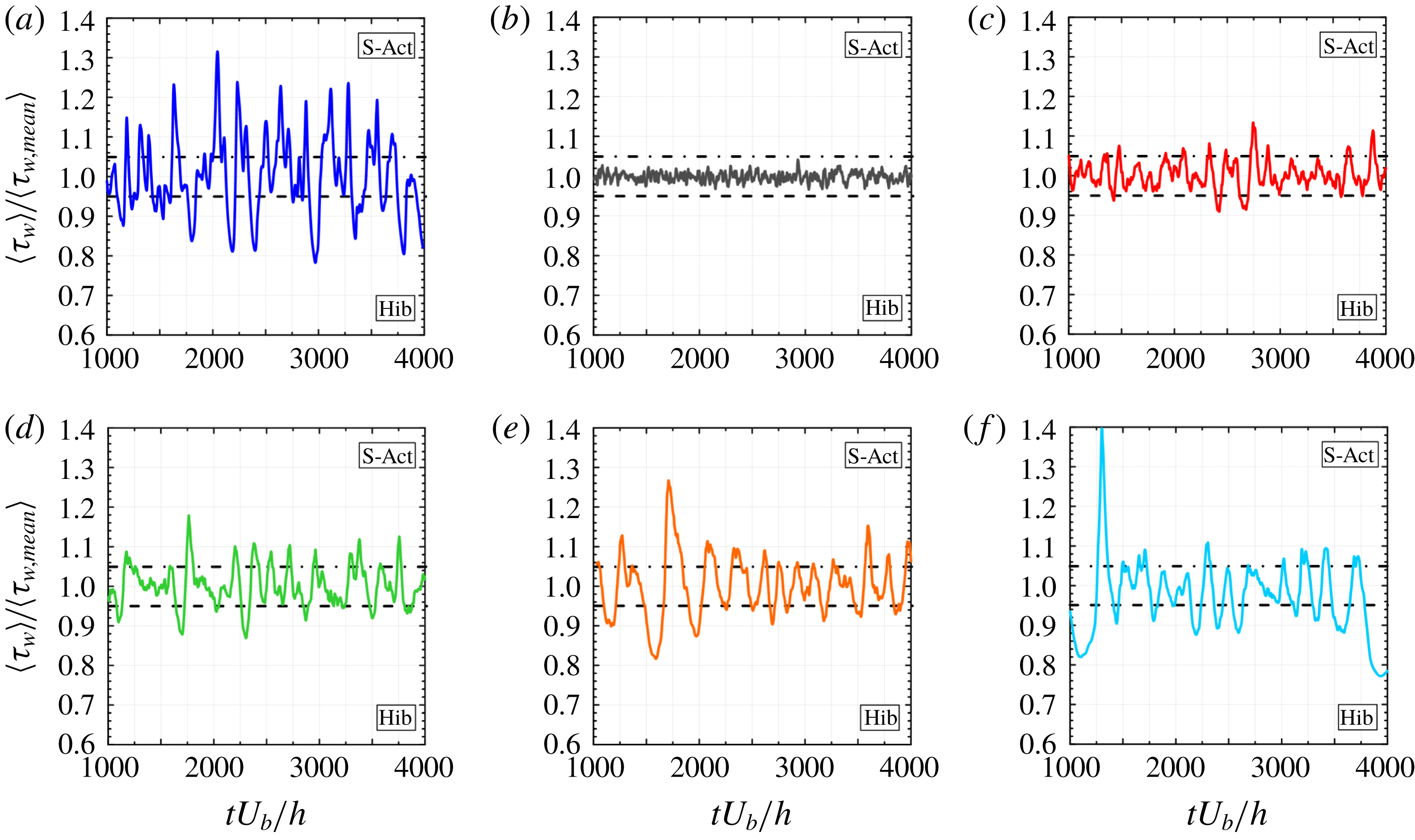
The dynamics of the alternation between hibernating and active turbulence can be clearly identified from the evolution in time (made dimensionless by
 $U_{b}$
and
 $h$
;
 $tU_{b}/h$
) of the spatial average of the shear stress at the wall,
 $\langle \unicode[STIX]{x1D70F}_{w}\rangle$
(in which ‘
 $\langle ~\rangle$
’ indicates the
 $x$
–
 $y$
spatial average), scaled with its time-averaged value,
 $\langle \unicode[STIX]{x1D70F}_{w,mean}\rangle$
(the shear stress is given by the
 $x$
–
 $y$
component of equation (2.2) evaluated at both walls). To provide a symmetric picture of this dynamics, we split the flow variations into three states: strong-active turbulence (S-Act), moderate-active turbulence (M-Act), and hibernating turbulence (Hib). From a review of the previous analysis (Xi & Graham Reference Xi and Graham2010; Pereira et al.
Reference Pereira, Mompean, Thais, Soares and Thompson2017b
), we decided to adopt a threshold of 0.05 in the standard deviation of the mean wall shear stress to delimit the three states. Therefore, the flow is considered in a hibernating state if
 $\langle \unicode[STIX]{x1D70F}_{w}\rangle <0.95\langle \unicode[STIX]{x1D70F}_{w,mean}\rangle$
(region below the dashed lines). The strong-active turbulence is the counterpart of the hibernation subregime, i.e.
 $\langle \unicode[STIX]{x1D70F}_{w}\rangle >1.05\langle \unicode[STIX]{x1D70F}_{w,mean}\rangle$
(region above the dash-dotted lines) while the moderate-active turbulence is delimited in the range
 $0.95\leqslant \langle \unicode[STIX]{x1D70F}_{w}\rangle /\langle \unicode[STIX]{x1D70F}_{w,mean}\rangle \leqslant 1.05$
.
Evolution in time (made dimensionless by
 $U_{b}$
and
 $h$
;
 $tU_{b}/h$
) of the
 $x$
–
 $y$
plane average wall shear stress,
 $\langle \unicode[STIX]{x1D70F}_{w}\rangle$
, normalised by its time-averaged value,
 $\langle \unicode[STIX]{x1D70F}_{w,mean}\rangle$
, for: (a)
 $Re_{b}=5750$
,
 $Wi_{b}=41$
,
 $L=100$
(
 $Re_{\unicode[STIX]{x1D70F}0}=180$
,
 $Wi_{\unicode[STIX]{x1D70F}0}=230$
,
 $L=100$
; viscoelastic turbulence at MDR subregime); (b)
 $Re_{b}=2830$
(
 $Re_{\unicode[STIX]{x1D70F}0}=180$
; fully Newtonian turbulent flow); (c)
 $Re_{b}=1250$
(
 $Re_{\unicode[STIX]{x1D70F}0}=88.06$
; Newtonian transition to turbulence); (d)
 $Re_{b}=1100$
(
 $Re_{\unicode[STIX]{x1D70F}0}=78.75$
; Newtonian transition to turbulence); (e)
 $Re_{b}=1000$
(
 $Re_{\unicode[STIX]{x1D70F}0}=72.44$
; Newtonian transition to turbulence); (f)
 $Re_{b}=950$
(
 $Re_{\unicode[STIX]{x1D70F}0}=69.26$
; Newtonian transition to turbulence). Spatial averages are taken at the wall plane. The mean value is computed considering the time interval shown,
 $tU_{b}/h$
 $\in [1000,4000]$
, where the lower bound is chosen to avoid the initial statistically transient evolution of the flow. The flow is considered in a hibernating state if
 $\langle \unicode[STIX]{x1D70F}_{w}\rangle <0.95\langle \unicode[STIX]{x1D70F}_{w,mean}\rangle$
(region below the dashed lines). The strong-active turbulence is the counterpart of the hibernation subregime, i.e.
 $\langle \unicode[STIX]{x1D70F}_{w}\rangle >1.05\langle \unicode[STIX]{x1D70F}_{w,mean}\rangle$
(region above the dash-dotted lines). The moderate-active turbulence is delimited in the range
 $0.95\leqslant \langle \unicode[STIX]{x1D70F}_{w}\rangle /\langle \unicode[STIX]{x1D70F}_{w,mean}\rangle \leqslant 1.05$
.

Figure 1 displays this evolution for the different cases considered here. Figure 1(a) shows a viscoelastic turbulent flow evolution corresponding to an MDR scenario that has already been explored in the literature (Xi & Graham Reference Xi and Graham2010; Pereira et al.
Reference Pereira, Mompean, Thais, Soares and Thompson2017b
). This panel shows a clear alternation between hibernating and strong-active turbulence where the wall shear stress differs from its mean value by more than
 $5\,\%$
. Figure 1(b) presents the corresponding fully turbulent Newtonian flow at the same value of the friction Reynolds number,
 $Re_{\unicode[STIX]{x1D70F}0}=180$
. In this case, the dynamics does not present the dual states of hibernation and strong-active turbulence.
A totally different path can be followed to produce turbulence statistics of the same nature as figure 1(a) starting from a fully turbulent flow, such as the one presented in figure 1(b). Comparing the sequence of decreasing Reynolds numbers represented by figure 1(c–f), we can observe how the decrease of inertia induces the appearance of a flow character, whose fingerprint is the alternation between hibernation and strong-active states, passing through moderate-active states in the process. During this process of Reynolds-number decrease, we notice an increase in the standard deviation of
 $\langle \unicode[STIX]{x1D70F}_{w}\rangle /\langle \unicode[STIX]{x1D70F}_{w,mean}\rangle$
. This point cannot be overemphasised. Figure 1 illustrates how, by decreasing
 $Re_{b}$
or increasing elastic effects (from a Newtonian fluid to a FENE-P one with
 $Wi_{b}=41$
and
 $L=100$
), we can arrive at turbulent regimes that show similar dynamic behaviour in the sense of the alternation between strong-active and hibernating states. Adopting a threshold of
 $0.95$
, we notice, by comparing figure 1(a) and (e), similar frequencies of appearance of hibernation states, with similar durations. In addition, the peaks and valleys of the strong-active and the hibernating states are of the same approximate values. When
 $Re_{b}$
is decreased to
 $Re_{b}=950$
, as shown in figure 1(f), we did not find any substantial differences in the frequency or amplitude of the dimensionless stress at the wall. However, we did find strong peaks and valleys events, such as the ones that occurred in times
 $tU_{b}/h\approx 1300$
and
 $tU_{b}/h\approx 3935$
.
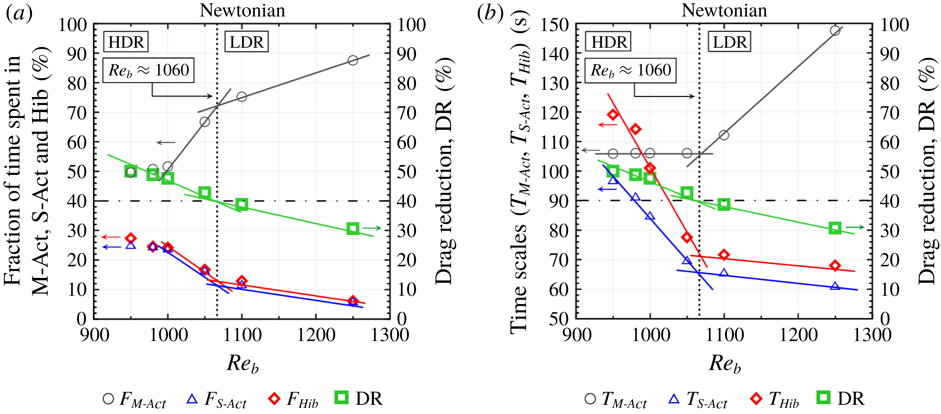
The results illustrated in figure 1 can be translated into a deeper layer of quantitative entities, as presented in figure 2. This figure is the Reynolds-number counterpart of the Weissenberg number presented in figure 2 of Xi & Graham (Reference Xi and Graham2010). Pereira et al. (Reference Pereira, Mompean, Thais, Soares and Thompson2017b
) have also reported similar results (figure 4f therein) for the viscoelastic turbulence in a Couette geometry. The quantities that are displayed against the Reynolds number are time scales (
 $T$
) and time fractions (
 $F$
). Because we have additional information due to the split of the active turbulence subregime, we have separated time fractions from time scales in figure 2(a) and (b), respectively. The time scales,
 $T_{Hib}$
(hibernation),
 $T_{S\text{-}Act}$
(strong activation) and
 $T_{M\text{-}Act}$
(moderate activation), are computed by taking the average of the intervals where the states remain in each of the three classes. The time fractions are obtained from the relative time spent inside a specific class,
 $F_{Hib}$
,
 $F_{S\text{-}Act}$
and
 $F_{M\text{-}Act}$
. Hence, these quantities can be mathematically defined as
 $T_{l}=\sum _{n=1}^{N_{l}}\unicode[STIX]{x0394}t_{l,n}/N_{l}$
and
 $F_{l}=\sum _{n=1}^{N_{l}}\unicode[STIX]{x0394}t_{l,n}/\unicode[STIX]{x0394}t_{total}$
, where
 $T_{l}$
and
 $F_{l}$
denote, respectively, the time scale and the time fraction related to a class
 $l$
(where
 $l$
can be equal to Hib, S-Act or M-Act),
 $N_{l}$
represents the number of intervals spent inside
 $l$
,
 $n$
indicates each interval of
 $l$
,
 $\unicode[STIX]{x0394}t_{l,n}$
is the time spent in each interval of
 $l$
, and
 $\unicode[STIX]{x0394}t_{total}$
is the total time interval of the simulation.
An important aspect of the result reported by Pereira et al. (Reference Pereira, Mompean, Thais, Soares and Thompson2017b
) is the slope change that occurs for the time scales and fractions at a critical Weissenberg number corresponding to
 $\text{DR}=40\,\%$
. Analogously to this elastic effect, we found a corresponding inertial effect, i.e. a remarkable change in the behaviours of time scales and time fractions at a critical Reynolds-number value that lies within the range
 $1050<Re_{b}<1100$
(or, more precisely,
 $Re_{b}\approx 1060$
). This range is clearly inside the transitional Reynolds-number extent (
 $950<Re_{b}<2500$
).
It would be interesting to obtain an objective criterion to delimit the two subregimes displayed in figure 2 (
 $950<Re_{b}<1060$
and
 $1060<Re_{b}<2500$
) that could be considered the Newtonian transitional counterpart of the viscoelastic turbulence LDR–HDR transition. The title of the article presented by Whalley et al. (Reference Whalley, Park, Kushwaha, Dennis, Graham and Poole2017) has already indicated the need for such an entity. Fortunately, an alternative form of computing the DR can be obtained from the energy budget analyses that was previously developed by Thais et al. (Reference Thais, Gatski and Mompean2013a
). More specifically, because the DR is directly linked with the weakening of turbulence,
 $\text{DR}$
can be calculated as the reduction of the peak magnitude of the production of turbulent kinetic energy (
 $P_{m}^{+}$
) against the wall distance (
 $z^{+}$
), in the statistically steady state (the superscript ‘
 $+$
’ indicates the wall-unit normalisation). This energy exchange term acts as a sink of mean kinetic energy to the turbulent kinetic energy, which is defined as the double dot product between the Reynolds stress tensor (
 $\unicode[STIX]{x1D749}_{R}^{+}\equiv \overline{\boldsymbol{u}^{\prime }\boldsymbol{u}^{\prime }}^{+}$
) and the mean rate-of-strain tensor (
 $\overline{\unicode[STIX]{x1D64E}^{+}}$
), i.e.
 $P_{m}^{+}=-\unicode[STIX]{x1D749}_{R}^{+}\,\mathbf{: }\,\overline{\unicode[STIX]{x1D64E}^{+}}$
. (The double dot product of two generic second-order tensors
 $\unicode[STIX]{x1D63C}$
and
 $\unicode[STIX]{x1D63D}$
is the inner product of these tensors; in index notation, the double dot product is obtained by the contraction on their corresponding indices,
 $\unicode[STIX]{x1D608}_{ij}\unicode[STIX]{x1D609}_{ij}$
.) Therefore, thanks to this direct proportionality, we can alternatively define a DR from a energy budget standpoint as
 $$\begin{eqnarray}\displaystyle \text{DR}=\left(1-\frac{\langle {P_{m,max}}^{+}\rangle }{\langle {P_{m,max}^{NFT}}^{+}\rangle }\right)\times 100\;[\%], & & \displaystyle\end{eqnarray}$$
where
 $\langle {P_{m,max}}^{+}\rangle$
is the maximum value of
 $\langle P_{m}^{+}\rangle$
relative to the Newtonian transitional case (or to the viscoelastic case, in a non-Newtonian scenario) and
 $\langle {P_{m,max}^{NFT}}^{+}\rangle$
is the peak magnitude of
 $\langle P_{m}^{+}\rangle$
related to the Newtonian fully turbulent channel flow, which in turn does not vary with
 $Re_{b}$
(
 $\langle {P_{m,max}^{NFT}}^{+}\rangle \approx 0.245$
; see also figure 9 in Appendix A). This method of computing DR is suitable to provide a general expression that can be used in Newtonian transitional flows and viscoelastic turbulent flows. More specifically, for viscoelastic turbulent flows, the DR levels obtained from equation (3.1) are similar to those given by the classical DR definition (equation 31 in Housiadas & Beris Reference Housiadas and Beris2013), which can be verified by taking into account all the DNS performed by our research group (Thais et al.
Reference Thais, Gatski and Mompean2012, Reference Thais, Gatski and Mompean2013a
,Reference Thais, Gatski and Mompean
b
; Pereira Reference Pereira2016; Pereira et al.
Reference Pereira, Mompean, Thais and Soares2017a
,Reference Pereira, Mompean, Thais, Soares and Thompson
b
,Reference Pereira, Mompean, Thais and Thompson
c
,Reference Pereira, Mompean, Thompson and Soares
d
, Reference Pereira, Mompean and Soares2018). Profiles of
 $\langle P_{m}^{+}\rangle$
as a function of
 $z^{+}$
are shown in Appendix A (figure 9).
Dynamic features of moderate-active (black circles), strong-active (blue triangles) and hibernating (red diamonds) states as functions of the Reynolds number: (a) time fractions
 $F_{M\text{-}Act}$
,
 $F_{S\text{-}Act}$
and
 $F_{Hib}$
; and (b) time scales
 $T_{M\text{-}Act}$
,
 $T_{S\text{-}Act}$
and
 $T_{Hib}$
. These quantities exhibit a remarkable change of slope near a critical Reynolds number revealing two different subregimes. These subregimes are embedded with similar features as the ones associated with HDR and LDR in turbulent viscoelastic flows. The green squares are obtained from an alternative method of computing DR that encompasses Newtonian turbulence and are the same for both panels. The dotted line of
 $Re_{b}\approx 1060$
corresponds to
 $\text{DR}=40\,\%$
, the usual limit that separates HDR and LDR in drag-reducing viscoelastic turbulent flows.

The green square points in figure 2 denote the DR values computed from equation (3.1). On decreasing the Reynolds number, DR increases, i.e. the effect of decreasing inertia is similar to what is obtained from increasing elasticity in viscoelastic turbulence. More strikingly, when adopting the usual viscoelastic value of
 $\text{DR}=40\,\%$
as a criterion for the boundary of the LDR and HDR subregimes, now in a Newtonian transitional context, we found a corresponding critical Reynolds number of
 $Re_{b,c}\approx 1060$
, a value in the possible range of the slope change behaviour concerning time scales and time fractions discussed above. For clarity,
 $Re_{b,c}$
is represented by a vertical dotted line in both panels of figure 2.
From figure 2(a) we notice that the results for time fraction of hibernating and strong-active turbulence are almost coincident throughout the LDR and HDR subregimes. Interestingly, both curves tend to the value of 25 % in the limit of non-laminar small
 $Re_{b}$
. The same trend was obtained by Xi & Graham (Reference Xi and Graham2010) and Pereira et al. (Reference Pereira, Mompean, Thais, Soares and Thompson2017b
) for the hibernating time fraction in the case of viscoelastic turbulence in the limit of high
 $Wi_{b}$
. It is worth noting that Xi & Graham (Reference Xi and Graham2010) used a minimal flow unit (MFU) approach, and Pereira et al. (Reference Pereira, Mompean, Thais, Soares and Thompson2017b
) examined the turbulence in the Couette geometry, which grants this result a general character. The splitting of the active turbulence has revealed that the extreme situations have
 ${\approx}50\,\%$
of the time fraction in this limit while the moderate-active states occupy the other half. For the Reynolds-number range that we analysed,
 $F_{Hib}$
and
 $F_{S\text{-}Act}$
are decreasing functions of
 $Re_{b}$
, while
 $F_{M\text{-}Act}$
is an increasing function of the Reynolds number. From figure 2(a) we expect a saturation in this tendency where hibernation and strong-active states would be a rare event.
Figure 2(b) shows a growth of the time scales associated with hibernation and strong-active states as inertia is reduced. Entering the HDR subregime, the impact of lowering the Reynolds number on these time scales is even stronger. The difference between
 $T_{Hib}$
and
 $T_{S\text{-}Act}$
is related to stronger peaks during the strong-active turbulence than in the hibernating state, in the period analysed. It is remarkable that
 $T_{M\text{-}Act}$
is not sensitive to changes in inertia in the HDR subregime but, when entering the LDR subregime towards the fully turbulent flow,
 $T_{M\text{-}Act}$
presents a positive correlation with
 $Re_{b}$
, which was expected.
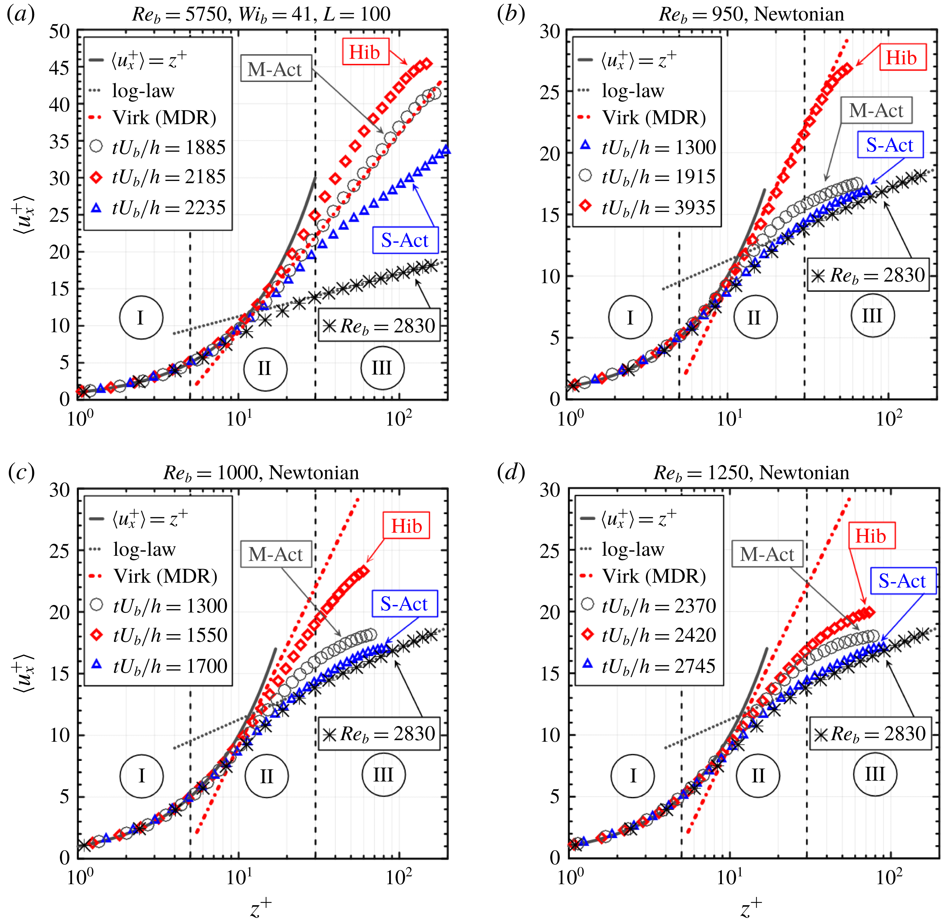
Instantaneous velocity profile obtained for the viscoelastic case analysed in the present work (
 $Re_{b}=5750$
,
 $Wi_{b}=41$
,
 $L=100$
; or
 $Re_{\unicode[STIX]{x1D70F}0}=180$
,
 $Wi_{\unicode[STIX]{x1D70F}0}=230$
,
 $L=100$
) and flows corresponding to the Newtonian transition to turbulence at three values of Reynolds number,
 $Re_{b}=950$
(
 $Re_{\unicode[STIX]{x1D70F}0}=69.26$
),
 $Re_{b}=1000$
(
 $Re_{\unicode[STIX]{x1D70F}0}=72.44$
),
 $Re_{b}=1250$
(
 $Re_{\unicode[STIX]{x1D70F}0}=88.06$
). For each case, three particular dimensionless times are chosen to represent hibernating, moderate-active and strong-active states. The time-averaged velocity profile obtained from
 $Re_{b}=2830$
(black asterisks), the log law (grey dotted line), the MDR asymptote (red dash-dotted line) and the viscous sublayer law (grey line) are plotted as references. Regions I, II and III correspond to the standard Newtonian limits for the viscous sublayer, buffer layer and log-law region, respectively.

Another aspect of the transitional regime can be explored by the analysis of the instantaneous velocity profiles, as is done in figure 3. The viscoelastic case considered in the present work with
 $Re_{b}=5750$
,
 $Wi_{b}=41$
and
 $L=100$
together with Newtonian results for three Reynolds numbers inside the transitional regime,
 $Re_{b}=950$
,
 $Re_{b}=1000$
and
 $Re_{b}=1250$
, are displayed in figure 3. In each flow, three particular instants were selected to represent hibernating, moderate-active and strong-active states. In addition, the theoretical velocity profiles associated with the Virk’s law (red dash-dotted line), the log-law (grey dotted line) and viscous sublayer law (grey line) are displayed to provide references for the analyses. Another important reference is the time-averaged velocity profile corresponding to
 $Re_{b}=2830$
(black asterisks), which shows that, at this level of Reynolds number, the usual path from the viscous sublayer to the Prandtl–von Kármán profile (log law) is attained.
An important fingerprint concerning the drag-reducing viscoelastic turbulence is shown in figure 3(a). There we can notice that the instantaneous velocity profile corresponding to the hibernating state surpasses the Virk’s profile. From the perspective of dynamics between hibernating and strong-active states, this outcome was logically expected. The reason for this expectation is due to the fact that the Virk’s law is a result that is associated with a mean (time-averaged) velocity profile. Therefore, given that this mean occurs with a quite large variance, the hibernating state must surpass the MDR. This fact does not change the status of the MDR being a maximum drag reduction state; it simply enforces that this is a mean result. It is worth noticing that the moderate-active state represented in figure 3(a) has a velocity profile in agreement with the Virk’s law. In this sense, the result obtained here is conceptually different from the cases reported in figure 2 of Graham (Reference Graham2014) and discussed by White, Dubief & Klewicki (Reference White, Dubief and Klewicki2012) and Elbing et al. (Reference Elbing, Perlin, Dowling and Ceccio2013), since they are related to cases where the time-averaged velocity profile is obtained. From the viewpoint of the recent study presented by Choueiri et al. (Reference Choueiri, Lopez and Hof2018), it still remains to determine if this MDR state is due to elasto-inertial instabilities.
The examination of figure 3(d) (
 $Re_{b}=1250$
), 3(c) (
 $Re_{b}=1000$
) and 3(b) (
 $Re_{b}=950$
) reveals that the instantaneous hibernating velocity profile becomes farther from the Prandtl–von Kármán profile as the Reynolds number is decreased in the laminar–turbulent Newtonian transitional range. On the other hand, strong-active states keep their profiles rather close to the log-law one, and the moderate-active profiles do not change that much either. This last observation is in contrast to the viscoelastic case shown in figure 3(a), where even the strong-active profile has considerably detached from the classical Newtonian turbulent profile.
Another important result, which is representative of the common nature of the Newtonian transitional regime and the drag-reducing viscoelastic turbulence, is shown in figure 3(b); this corresponds to
 $Re_{b}=950$
, with the instantaneous velocity profile associated with the hibernating state. This coincidence between this Newtonian profile and the Virk’s law is impressive, corroborating the recent result obtained by Alizard & Biau (Reference Alizard and Biau2019). Because the Virk’s profile is a cornerstone of the analysis of drag-reducing viscoelastic turbulence, which is associated with the maximum drag that can be attained, this coincidence has far-reaching consequences. This finding suggests that the Virk’s law is a broader result, a phenomenon associated with general turbulence and not restricted to the turbulence of viscoelastic fluids. The conjecture outlined next is that this state is connected to a set of conditions that are close to the minimum flow strength necessary to keep the flow out of the laminar regime. In other words, taking a high-Reynolds-number flow where perturbations are highly amplified to lead to a fully turbulent flow as reference, the decrease of
 $Re_{b}$
leads to states of less and less amplification power. At this point, it is important to report that the Reynolds-number value of
 $Re_{b}=950$
is very near the lower bound for transition, since for
 $Re_{b}=945$
the perturbation introduced was dissipated and a laminar regime was obtained after an unsteady period. Before achieving the laminar regime where perturbations are damped and die due to viscous effects, there comes the transition regime where an alternation between hibernating and active states characterises the dynamics of the motion. The hibernating state, where turbulence is weak, has a lower bound that limits its existence, i.e. the weakest form of non-laminar flow. The results presented here suggest that this state is connected to the Virk’s law with no distinction between Newtonian and viscoelastic turbulence. This lower bound limit does not necessarily mean that the velocity profile does not surpass the Virk’s law. As in the viscoelastic case, probably the solutions can visit spaces between the lower branch and the laminar flow, but they remain in the vicinity of the former.
Even with this lowest Reynolds-number value,
 $Re_{b}=950$
, we can find a strong-active state where the instantaneous velocity profile is close to the Prandtl–von Kármán profile. In other words, the oscillation dynamics of the flow at this level of Reynolds number covers the whole spectrum of possibilities, including the boundaries of the transitional regime. As the Reynolds number is increased, hibernation detaches and distances from the Virk’s law profile, while the strong-active state associated coincides even more with the fully turbulent log-law profile.
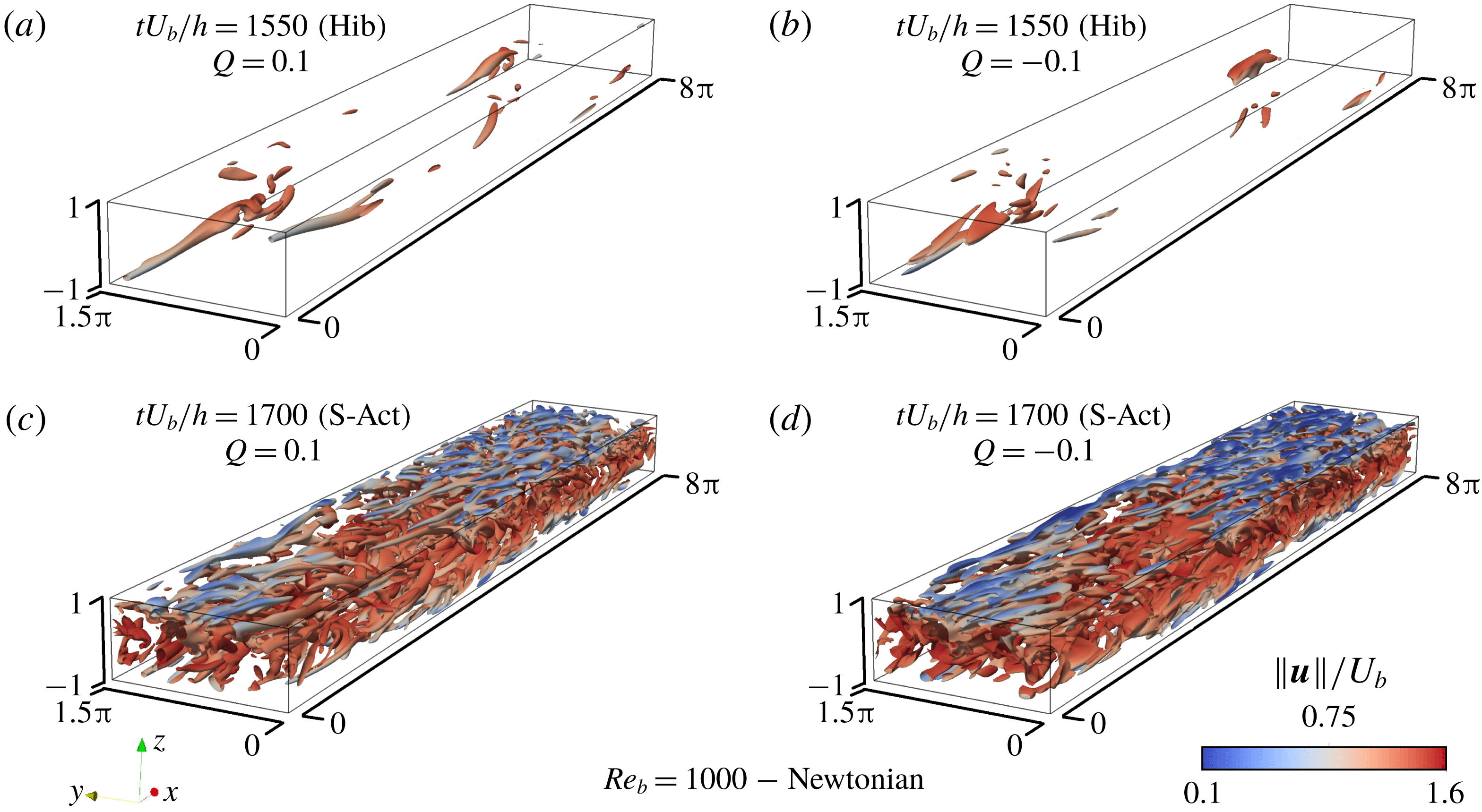
Elliptical and hyperbolic structures as captured by the
 $Q$
-criterion, coloured by the dimensionless velocity magnitude,
 $\Vert \boldsymbol{u}\Vert /U_{b}$
(where
 $\boldsymbol{u}$
is the velocity vector and
 $U_{b}$
the bulk velocity), for a bulk Reynolds number
 $Re_{b}=1000$
. The chosen thresholds have the same magnitude,
 $\Vert Q\Vert =0.1$
, to illustrate the symmetric nature with respect to the parabolic state where
 $Q=0$
. The instants of evaluation of the structures were selected with respect to the evolution in time of the normalised shear stress at the wall. The dimensionless time of
 $tU_{b}/h=1550$
corresponds to a typical hibernating state, while a typical strong-active turbulence state is reached at
 $tU_{b}/h=1700$
, based on the evolution of the dimensionless shear stress at the wall shown in figure 1(d). A movie concerning this flow case is available online at https://anselmopereira.net/videos/.

Interestingly, the moderate-active state seems to exhibit a log-law profile parallel to the fully Newtonian one after a certain value of
 $Re_{b}$
in the same fashion as the velocity profiles of the viscoelastic-turbulent-LDR subregime, while the velocity of the hibernating state exhibits a viscoelastic-turbulent-HDR-like profile.
Taking the transitional Newtonian flow at
 $Re_{b}=1000$
as the focus of our analysis, figure 4 shows turbulent structures at two values of dimensionless time taken from the evolution shown in figure 1(e), one of which belongs to a hibernating state (figure 4
a and 4
b), while the other is in a strong-active state (figure 4
c and 4
d). The turbulent structures are captured by the
 $Q$
-criterion (see Hunt, Wray & Moin Reference Hunt, Wray and Moin1988). The vortical (or elliptical) and extensional (or hyperbolic) structures are defined as the respective positive and negative values of the second invariant of the velocity gradient tensor, computed for incompressible flows by
 $Q=\frac{1}{2}(\Vert \unicode[STIX]{x1D652}\Vert ^{2}-\Vert \unicode[STIX]{x1D64E}\Vert ^{2})$
, where
 $\Vert \unicode[STIX]{x1D652}\Vert$
and
 $\Vert \unicode[STIX]{x1D64E}\Vert$
denote the Euclidean norms of
 $\unicode[STIX]{x1D652}$
and
 $\unicode[STIX]{x1D64E}$
; the Euclidean norm of a generic second-order tensor
 $\unicode[STIX]{x1D63C}$
is
 $\Vert \unicode[STIX]{x1D63C}\Vert =\sqrt{\text{tr}(\unicode[STIX]{x1D63C}\boldsymbol{\cdot }\unicode[STIX]{x1D63C}^{\text{T}})}$
. In addition to the traditional picture of a positive
 $Q$
value (elliptical regions), which is commonly connected to vortex activity, we also show the corresponding hyperbolic set of structures by exhibiting isovalues associated with
 $Q=-0.1$
(a movie concerning this flow case is available online at https://anselmopereira.net/videos/). The similarity in structure activity with the elliptical counterpart,
 $Q=0.1$
, is noteworthy (see also Pereira et al.
Reference Pereira, Mompean, Thais and Soares2017a
). Alternative approaches for the visualisation of turbulence activity can be found in Fu et al. (Reference Fu, Iwaki, Motozawa, Tsukara and Kawaguchi2015), who have used instantaneous flow fields of the second invariant of the Reynolds stress tensor and time trace of velocity fluctuations. Tuckerman et al. (Reference Tuckerman, Kreilos, Schrobsdorff, Scneider and Gibson2014) employed contours of streamwise vorticity, spanwise and transverse velocities, and Xiong et al. (Reference Xiong, Tao, Chen and Brandt2015) used isocontours of transverse velocity. The lack of elliptical and hyperbolic structures in the hibernating state when compared to the strong-active state was explored by Pereira et al. (Reference Pereira, Mompean, Thompson and Soares2017d
). However, in contrast to that work, in which the weakening of turbulent structures was interpreted as a consequence of elastic effects, in this paper these same flow changes occur in a purely Newtonian transitional flow. In other words, the topological viewpoint also evidences important common features between the Newtonian transitional flow and the viscoelastic drag-reducing flow.
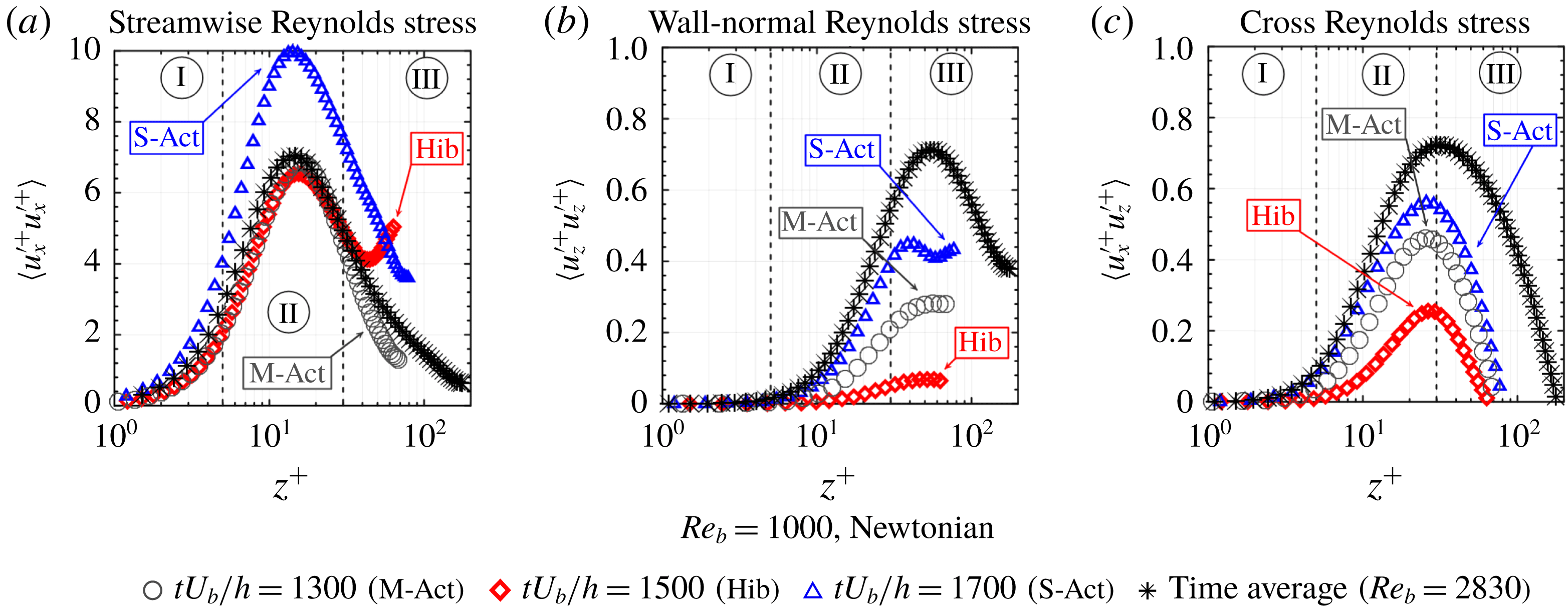
Spatial average quantities related to chosen instants that correspond to moderate-active (grey circles), strong-active (blue triangles) and hibernating (red diamonds) states as functions of the wall distance for the
 $Re_{b}=1000$
transitional case and the mean values for the
 $Re_{b}=2830$
fully turbulent case for comparison (black asterisks): (a) streamwise-normal Reynolds stress component; (b) wall-normal Reynolds stress component; and (c) shear Reynolds stress component.

Figure 5(a–c) shows that, in a hibernating state, the Reynolds stress tensor is significantly suppressed when compared to the strong-active state. This same result is found in viscoelastic turbulence. While the moderate-active state has a similar instantaneous velocity profile when compared to that in the strong-active state, figure 5(a) reveals that the streamwise Reynolds stress normal component is characterised by a straight relation between moderate-active turbulence and hibernating turbulence, especially in the viscous and buffer layers. The profile of the moderate-active state for the wall-normal stress component (figure 5
b) is approximately in the middle between hibernating and strong-active states. Again, the hibernating and strong-active states of the Newtonian transitional flow exhibit the HDR and LDR turbulent viscoelastic behaviour, respectively. More specifically, the peak magnitude of
 $\langle {u_{z}^{\prime }}^{+}{u_{z}^{\prime }}^{+}\rangle$
observed in the strong-active state is absent in the hibernating state.
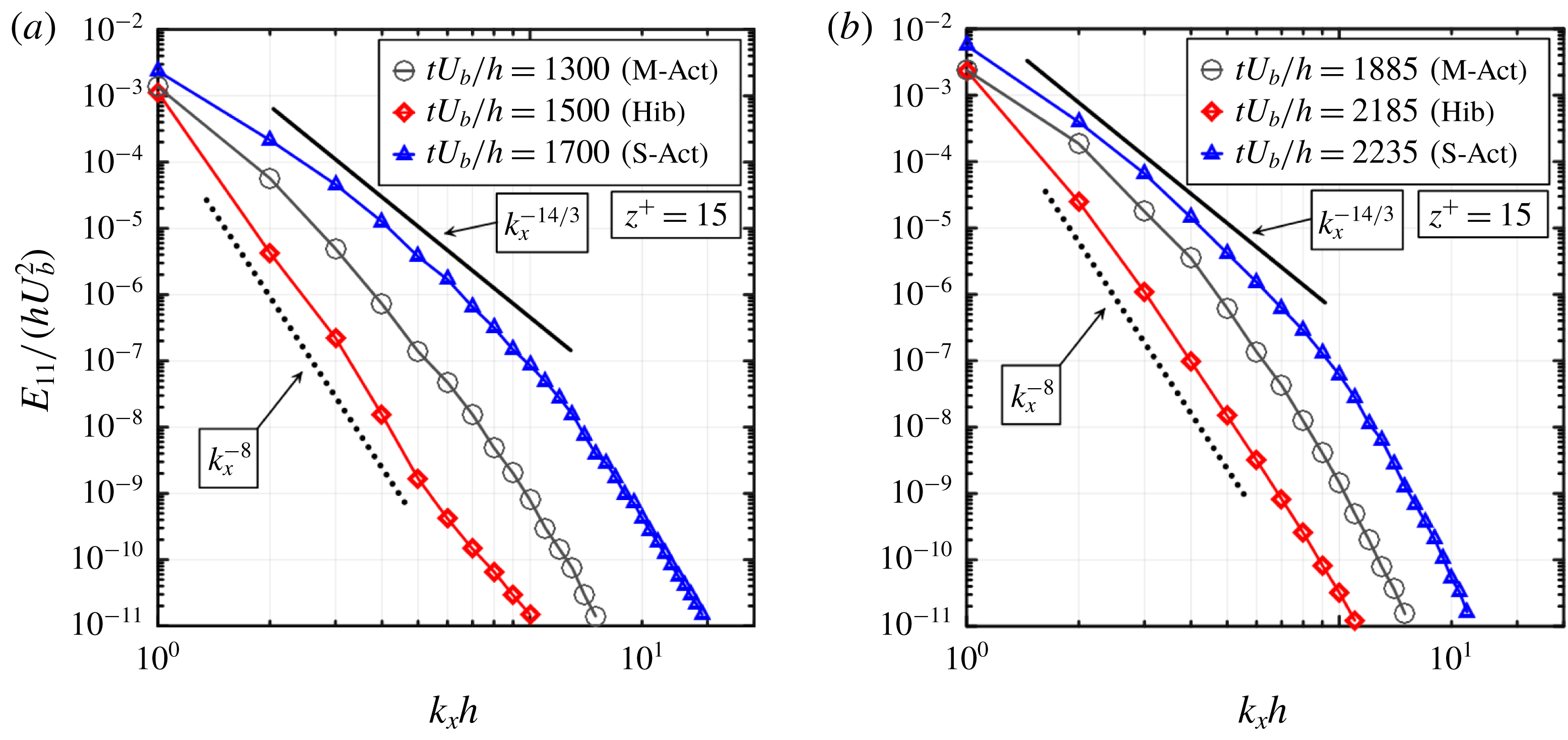
Longitudinal one-dimensional spectra of turbulent kinetic energy (made dimensionless by
 $hU_{b}^{2}$
) with respect to the dimensionless
 $x$
component of the wavenumber at position
 $z^{+}=15$
corresponding to the three states, moderate-active (black circles), strong-active (blue triangles) and hibernating (red diamonds): (a) for the Newtonian
 $Re_{b}=1000$
case; and (b) for the drag-reducing
 $Re_{b}=5750$
,
 $Wi_{b}=41$
,
 $L=100$
case in the MDR subregime. The full line indicates the slope of the strong-active state in the first part of the spectrum, while the dotted line indicates the slope of the hibernating state in the same part. The instants chosen to represent the hibernating, moderate-active and strong-active states for the drag-reducing viscoelastic turbulence were based on results presented in figure 1(b). The slopes obtained for the Newtonian and drag-reducing cases are in very good agreement.

Another result that reinforces the common nature of the transitional flow of a Newtonian fluid and the viscoelastic turbulent context concerns the spectra of turbulent kinetic energy. Figure 6 shows the longitudinal one-dimensional spectra of turbulent kinetic energy (made dimensionless by
 $hU_{b}^{2}$
),
 $E_{11}/(hU_{b}^{2})$
, as a function of the dimensionless
 $x$
component of the wavenumber vector,
 $k_{x}h$
, for the position located at
 $z^{+}=15$
. The similarities between the panels associated with the Newtonian transitional flow (
 $Re_{b}=1000$
) and the drag-reducing viscoelastic flow (
 $Re_{b}=5750$
,
 $Wi_{b}=41$
,
 $L=100$
) are again striking. The previously selected states chosen to represent the hibernating, moderate-active and strong-active turbulence for the Newtonian transition were again adopted. New representative instants associated with the evolution in time of the viscoelastic case (see figure 1
b) were selected to illustrate what is happening in each of these three states. First, we can notice that the typical
 $-14/3$
power-law exponent for drag-reducing flows (Dubief et al.
Reference Dubief, Terrapon and Soria2013; Thais et al.
Reference Thais, Gatski and Mompean2013b
; Watanabe & Gotoh Reference Watanabe and Gotoh2013), associated with the strong-active state, are found in the transitional flow for the corresponding strong-active state. In addition, both hibernating states exemplified in figure 6(a) and (b) also present a similar power-law exponent decay of
 $-8$
. Both decays, the
 $k_{x}^{-14/3}$
for the strong-active state, and the
 $k_{x}^{-8}$
for the hibernating state, were already found by Pereira et al. (Reference Pereira, Mompean, Thais, Soares and Thompson2017b
) in the context of the viscoelastic turbulent Couette flow. This character of exhibiting similar energy distribution among the different length scales for the different qualitative states – namely strong-active, moderate-active and hibernating states – reveals an impressive ubiquitous aspect of these states.
4 Concluding remarks
The present work explores results in a range where Newtonian laminar–turbulent transition and viscoelastic turbulence exhibit common features. In this regard, the upper and lower branches of the travelling wave solutions that appear after a critical Reynolds number in the Navier–Stokes equations are also present in viscoelastic drag-reducing dynamics. The results suggest that, while the Prandtl–von Kármán profile seems to be associated with the upper branch, the Virk’s profile seems to be associated with the lower branch. In other words, these two classes of flows seem to have the same limits and constitute upper and lower boundaries of drag (Waleffe Reference Waleffe2001), and, in this scenario, the viscoelastic MDR is also a maximum drag reduction in the Newtonian world, which would coincide with the weakest form of non-laminar flow. When the Reynolds number is high, the Newtonian turbulence associated with the upper-branch solution constitutes a stronger basin of attraction and, therefore, excursions out of this solution have a smaller amplitude and rarely visit the lower-branch solution. When
 $Re_{b}$
is decreased and the transitional regime is achieved, the lower branch is visited more often but, due to its strongly unstable nature, excursions out of this solution are common and the alternation between hibernating and active states is a fingerprint of the flow dynamics. In the case of the Newtonian
 $Re_{b}=950$
flow, we found hibernating states that obey the MDR profile and strong-active states that obey the Prandtl–von Kármán profile. In the case of the viscoelastic drag-reducing flow that we have analysed in the present work, we were able to infer the existence of trajectories from the lower-branch solution towards the laminar one, as identified by a hibernating state whose velocity profile is beyond the MDR limit. However, these trajectories return and fluctuate around the Virk’s profile. The general results that we have obtained in the present work show that viscoelastic drag-reducing flows can be understood as transitional.
Taking the Newtonian
 $Re_{b}=2830$
flow as a reference, conditions that present similarities from the statistical point of view can be reached by two different strategies: increasing elasticity (increasing
 $Wi_{b}$
and/or
 $L$
in a FENE-P fluid) or decreasing inertial effects (decreasing
 $Re_{b}$
). More specifically, a closer comparison between the
 $Re_{b}=1000$
Newtonian case and the
 $Re_{b}=5750$
,
 $Wi_{b}=41$
,
 $L=100$
FENE-P case unveiled striking similarities in the dynamics of the alternation between hibernating and active states, as well as in particular features of representative instants that correspond to hibernating, strong-active and moderate-active states. Because the explanation offered by Xi & Graham (Reference Xi and Graham2010) is based on the polymer dynamics during the cycle process, another mechanism must be considered to take place in the Newtonian turbulence transitional flow. In what follows, we present a possible explanation for the oscillation between hibernating and active states in this other situation.
Next, we offer a plausible explanation for the cycling mechanism that is able to address the main features of the common dynamics in Newtonian laminar–turbulent transition and viscoelastic turbulence. This explanation needs further investigation, to be confirmed. When the transitional regime is achieved, the alternation between hibernating and active states is a fingerprint of the flow dynamics. The moderate Reynolds number is able to amplify the perturbations until a point where an active state takes place. The formation of elliptical and hyperbolic structures is accompanied by an increase of the velocity gradient, especially near the wall (where the velocity vanishes). Therefore, the viscous stresses increase and they tend to suppress turbulence by weakening elliptical and hyperbolic structures, which decreases the velocity gradient and produces a hibernating state. This state decreases the viscous stresses, increasing the potential for perturbation amplification, returning to the initial point of the cycle.
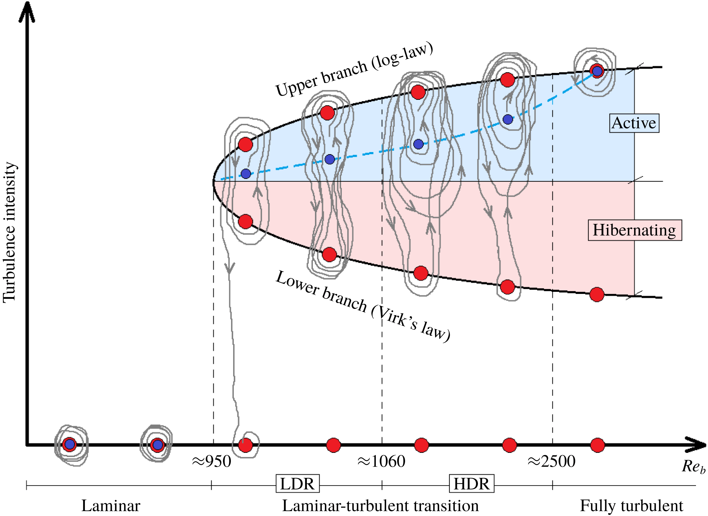
Schematic of the conjecture picture of the transitional dynamics with increasing Reynolds number. The red dots correspond to equilibrium states. Before the first critical Reynolds number (
 $Re_{b}\approx 950$
), only one equilibrium point is possible: the laminar one. Beyond this value, a bifurcation begins and three equilibrium points coexist for each Reynolds number: a laminar one, a lower-branch nonlinear travelling wave one and an upper-branch nonlinear travelling wave one. The blue dots indicate the state of highest probability of a solution to pass through, while the blue dashed line shows how these blue dots evolve as
 $Re_{b}$
increases. The grey lines with arrows indicate solution trajectories. A second critical Reynolds number (
 $Re_{b}\approx 1060$
) delimits the HDR–LDR subregimes. A third one is the lower boundary for a fully turbulent flow. The middle horizontal line of the bifurcation curve separate active-like states (near the upper branch) from hibernating-like states (near the lower branch).

Figure 7 shows a schematic that illustrates the conjecture of the transitional dynamics. This schematic can be seen as the Newtonian counterpart of figure 17 of Graham (Reference Graham2014) adding that perspective onto the diagram represented by figure 8 of Barkley (Reference Barkley2016). Figure 7 is a Reynolds number versus turbulence intensity graph with the traditional bifurcation curve that starts at a critical Reynolds number that limits the laminar–non-laminar regimes. The
 $Re_{b}$
ranges for laminar, transitional and fully turbulent regimes are indicated. The transitional regime is divided into high and low DR subregions. The grey lines indicate trajectories of the solutions. Among the possible states these trajectories pass by, three of them, represented by the red dots, constitute important references. The laminar state is a stable solution that is strictly stable below a second critical Reynolds number inside the transition regime, possibly the one that limits HDR and LDR regions. In the HDR subregimes, realisations where the laminar state is achieved, as illustrated in figure 15 of Graham (Reference Graham2014), are exemplified in figure 7. The upper and lower branches are connected with the nonlinear travelling wave solutions where the upper branch is associated with a higher turbulence intensity than the lower branch. The active and hibernating regions are delimited by an area that is under the influence of the upper- and lower-branch sets, respectively.
A general conjecture illustrated here is that, outside the transition regime, the strictly stable solutions, laminar and upper branch are strong attractors for low and high Reynolds numbers, respectively. On the other hand, the transitional range is marked by a significant importance of the lower-branch solution in the trajectory dynamics. The transitional regime would be characterised by intermittent orbits of solutions where the attraction exerted by the upper branch is not strong enough to avoid the trajectories visiting states near the unstable lower-branch solution (see Park, Shekar & Graham Reference Park, Shekar and Graham2018). These orbits can be heteroclinic, near-heteroclinic and homoclinic. As the Reynolds number is increased, the distance in state space between the stable and unstable solutions increases and the stable turbulent state of the upper branch strengthens its power of attraction, leading to a gradual migration of higher trajectory densities (whose barycentre is represented by the blue dots) towards this stable branch. In other words, for values of
 $Re_{b}$
in the transitional regime but near the laminar–transitional limit, it is more likely to have heteroclinic connections between the stable and unstable states. As the Reynolds number is increased, more orbits that are nearly heteroclinic appear and, less frequently, homoclinic orbits containing only the upper-branch solution.
A further increase in
 $Re_{b}$
increases the number of homoclinic orbits, making the heteroclinic connections less frequent. In this process, the fraction of time spent in hibernating states decreases. These periods correspond to the fraction of time that the solution trajectories spend in the hibernating region. After a certain threshold in the Reynolds number, the attraction of the upper branch leads to solutions that are not able to leave the vicinity of this stable attractor point and virtually only homoclinic orbit realisations are obtained. At this stage, the fully turbulent regime is achieved, and, consequently, the typical Prandtl–von Kármán velocity profile becomes the rule. In the opposite direction, near the laminar limit, where upper and lower branches are very close, active and hibernating states have a tendency to be equiprobable, since the stable and unstable solutions tend to coincide. Although the scenario illustrated by this schematic has some conjectures, it does not contradict any of the results obtained and offers a plausible and compact explanation that can contribute to the understanding of the laminar–turbulent transition.
Lastly, the rationale formulated above, as well as the results obtained in the present work, induce the thought that viscous effects (sometimes referred to as Lumley’s theory) are more likely to explain DR than the elastic effects (sometimes referred to de Gennes’ theory) because the cycling mechanism based on the opposition of viscous and inertial effects can explain the alternation of hibernating and strong-active turbulence in the DR regimes of viscoelastic turbulence and transition to Newtonian turbulence. However, as pointed in § 1, the recent studies on elasto-inertial turbulence (EIT) have unequivocally placed the subject of viscoelastic turbulence in general as a complex phenomenon where elasticity plays a fundamental role (see Dubief et al. Reference Dubief, Terrapon and Soria2013; Choueiri et al. Reference Choueiri, Lopez and Hof2018; Sid et al. Reference Sid, Terrapon and Dubief2018; Shekar et al. Reference Shekar, McMullen, Wang, McKeon and Graham2019).
5 Future perspectives
Besides the results that expose quantitative similarities between Newtonian laminar–turbulent transition and viscoelastic drag-reducing turbulence, a number of conjectures were open and need further investigation. Some of them are described below:
(i) Explore hibernating states in the lowest-Reynolds-number value where the Newtonian flow is non-laminar
 $(Re_{b}\approx 950)$
. This study would reveal, among other things, if profiles beyond the MDR asymptote can be achieved, as in the case of viscoelastic drag-reducing turbulent flows.
(ii) Investigate the dynamics of alternation between hibernating and active states in MFU and even smaller domains until the limit of one cell. The idea is to introduce the highest standard deviation possible to produce a scenario of higher probability of finding lower valleys of hibernating states and highest peaks of strong-active states.
(iii) Investigate the boundary between LDR and HDR in Newtonian laminar–turbulent transition. This investigation would answer whether the critical value established in the present result concerning the LDR–HDR limit is coincident or not (and in this second case, which one would be higher) with the result provided by the literature concerning the critical value for the stable–metastable interchange between laminar and upper-branch solutions. Since the coexistence of two critical values (one not discovered until this work) is unlikely, we believe that these values do coincide.
(iv) Compare Newtonian laminar–turbulent transition flows to viscoelastic drag-reducing turbulent flows at the same DR level (and for a wide range of
$\text{DR}$
).(v) Adapt the Newtonian transitional scheme made in the conclusions to viscoelastic drag-reducing cases parametrised by the Weissenberg number.
(vi) Investigate more extensively the connections between the hibernating state and HDR subregime, as well as between the active state and the LDR subregime. We found that the instantaneous velocity profiles obtained from a hibernating state have a tendency to exhibit an HDR character, even for hibernating states that come from an LDR subregime. The same connection with respect to the active state and HDR subregime applies. Therefore, the features of an instantaneous velocity profile seem to be associated with the state, while the subregime is a collection of states and, therefore, reveals a global character that weights more the states that are more frequent.


Acknowledgements
This research was granted access to the HPC resources of IDRIS under the allocations 2016-i20162a2277 and i100790 DARI A0032A10304 made by GENCI. The authors also would like to express their acknowledgement and gratitude to the Brazilian Scholarship Program ‘Science Without Borders’, managed by CNPq (National Council for Scientific and Technological Development), for partial financial support for this research. A.S.P. would like to thank the PSL Research University for its support under the program ‘Investissements d’Avenir’ launched by the French Government and implemented by the French National Research Agency (ANR) with the reference ANR-10-IDEX-0001-02 PSL.
Appendix A
A.1 The maximum drag reduction case
In the present work, six Newtonian transitional flows (
 $Re_{b}=950$
, 985, 1000, 1050, 1100 and 1250), as well as one Newtonian fully turbulent flow (
 $Re_{b}=2830$
) are compared with a FENE-P viscoelastic turbulent one in the MDR subregime (
 $Re_{b}=5750$
,
 $Wi_{b}=41$
,
 $L=100$
).
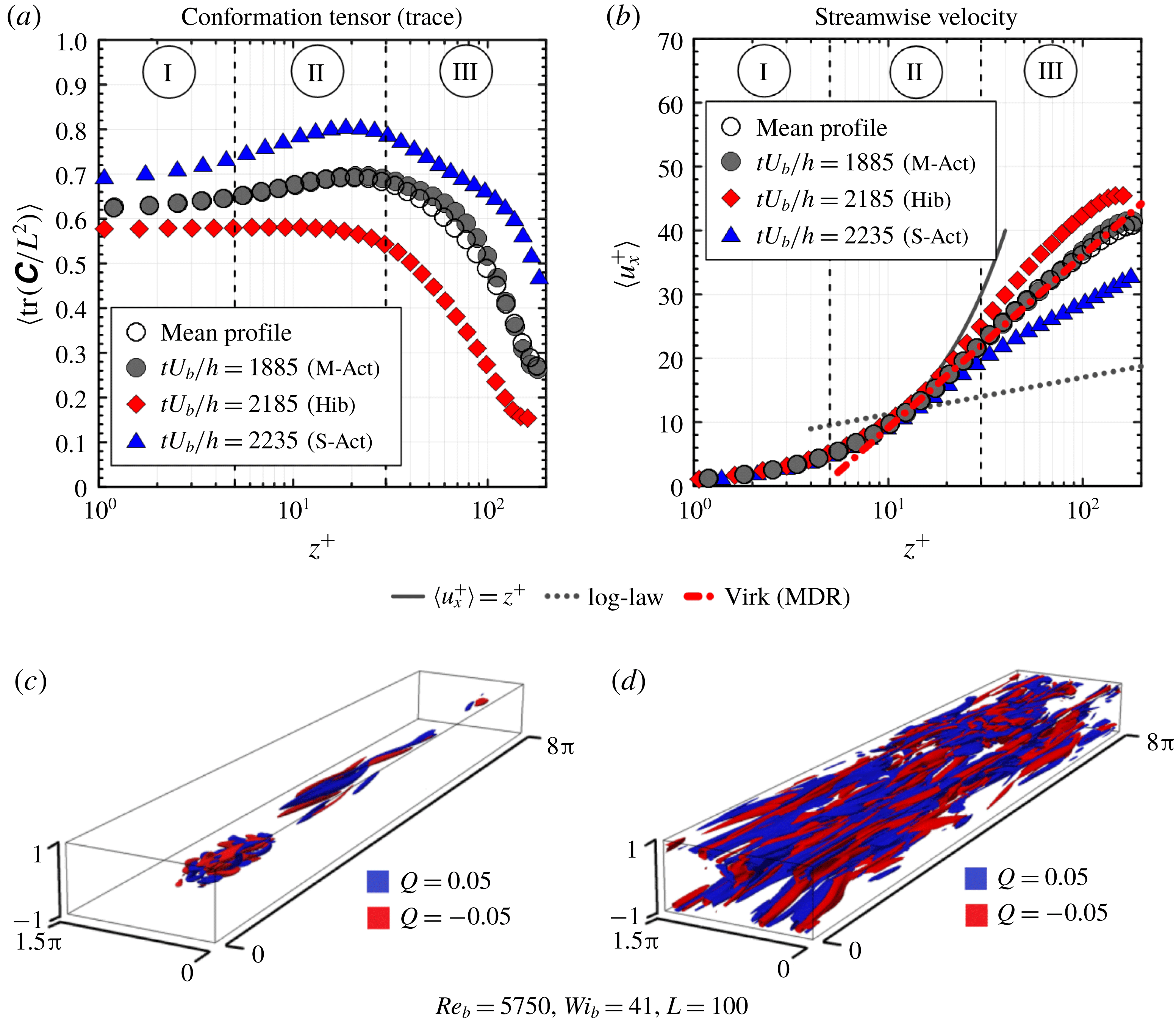
Regarding our viscoelastic case, in figure 8, instantaneous profiles of the relative polymer extension are plotted (
 $\langle \text{tr}(\unicode[STIX]{x1D63E})/L^{2}\rangle$
; figure 8
a) together with instantaneous streamwise velocity (
 $\langle u_{x}^{+}\rangle$
; figure 8
b). As discussed previously, each point in figure 8(a,b) is an average in the
 $x$
–
 $y$
plane along
 $z^{+}$
. The channel half-width is divided into three distinct regions: I (
 $0<z^{+}<5$
), II (
 $5<z^{+}<30$
) and III (
 $z^{+}>30$
). Three different dimensionless instants are considered: an instant for the strong-active state (S-Act) characterised by
 $\langle \unicode[STIX]{x1D70F}_{w}\rangle /\langle \unicode[STIX]{x1D70F}_{w,mean}\rangle >1.05$
(
 $tU_{b}/h=2235$
; blue solid triangles); an instant corresponding to the moderate-active state (M-Act), for which
 $0.95\leqslant \langle \unicode[STIX]{x1D70F}_{w}\rangle /\langle \unicode[STIX]{x1D70F}_{w,mean}\rangle \leqslant 1.05$
(
 $tU_{b}/h=1885$
; grey solid circles); and, finally, an instant related to the hibernating state (Hib) at which
 $\langle \unicode[STIX]{x1D70F}_{w}\rangle /\langle \unicode[STIX]{x1D70F}_{w,mean}\rangle <0.95$
(
 $tU_{b}/h=2185$
; red solid diamonds). Additionally, in figure 8(b), the theoretical velocity profiles associated with the Virk’s law (red dash-dotted line), the Prandtl–von Kármán log law (grey dotted line) and the viscous sublayer law (grey line) are displayed to provide references for the analyses. Another important reference is the time-averaged velocity profile (black circles), which is fitted by the Virk’s law. Finally, figure 8(c,d) shows three-dimensional turbulent structures (vortical in blue and extensional in red) defined by the
 $Q$
-criterion (
 $Q=\pm 0.05$
) flow classification Hunt et al. (Reference Hunt, Wray and Moin1988).
Polymers clearly appear more extended in the strongly active periods (
 $tU_{b}/h=2235$
, for instance), when the instantaneous velocity profile surpasses the Virk’s profile and the turbulent structures with
 $Q=\pm 0.05$
are more numerous. In contrast, in the hibernating periods (
 $tU_{b}/h=2185$
, for example), the molecules are in their least-stretched configuration, the instantaneous velocity profile moves towards the log law, and the structures with
 $Q=\pm 0.05$
almost vanish. It is also important to observe that, at
 $tU_{b}/h=1885$
, both
 $\langle \text{tr}(\unicode[STIX]{x1D63E})/L^{2}\rangle$
and
 $\langle u_{x}^{+}\rangle$
coincide with their respective time-averaged values.
(a) Average values in the
 $x$
–
 $y$
planes of the relative polymer stretching,
 $\langle \text{tr}(\unicode[STIX]{x1D63E})/L^{2}\rangle$
, as a function of the dimensionless wall distance,
 $z^{+}$
. (b) Average values in the
 $x$
–
 $y$
planes of the streamwise velocity,
 $\langle u_{x}^{+}\rangle$
, as a function of
 $z^{+}$
. (c,d) The three-dimensional structures represent isosurfaces of extensional (or hyperbolic) regions defined as the second invariant of the velocity gradient tensor (
 $Q$
-criterion). Two dimensionless instants are considered:
 $tU_{b}/h=2185$
(c) and
 $tU_{b}/h=2235$
(d).

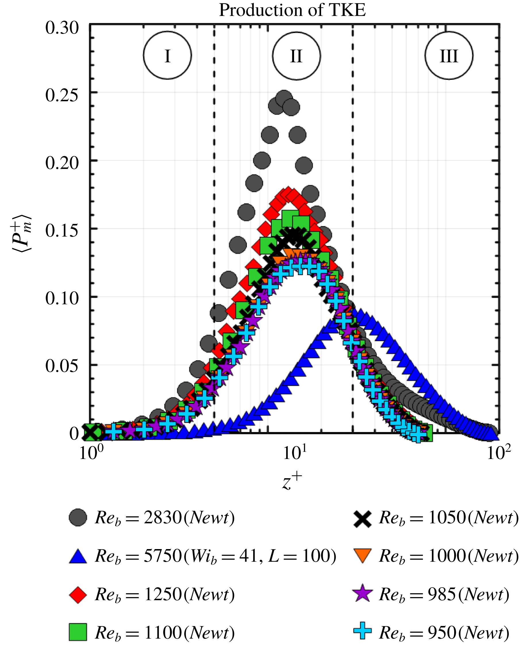
A.2 Alternative energy-based definition of drag reduction
An alternative DR definition is reported in the present work (equation (3.1)). This definition is based on the peak magnitude of the average in the
 $x$
–
 $y$
planes of the time-averaged production of turbulent kinetic energy (TKE),
 $\langle P_{m}^{+}\rangle$
, along
 $z^{+}$
. This curve is shown in figure 9 for all cases analysed here.
It is worth mentioning that the peak magnitude of
 $\langle P_{m}^{+}\rangle$
for Newtonian fully turbulent channel flows (
 $\langle {P_{m,max}^{NFT}}^{+}\rangle$
) does not depend on the Reynolds number. Hence, for Newtonian fully turbulent channel flows,
 $\langle {P_{m,max}^{NFT}}^{+}\rangle =0.245$
for any
 $Re_{b}$
. For both the Newtonian transitional and the viscoelastic cases, however, the maximum value of
 $\langle P_{m}^{+}\rangle$
(
 $\langle {P_{m,max}}^{+}\rangle$
) varies with
 $Re_{b}$
, as illustrated in figure 9:
 $\langle {P_{m,max}}^{+}\rangle =0.1225$
at
 $Re_{b}=950$
(
 $\text{DR}\approx 50\,\%$
);
 $\langle {P_{m,max}}^{+}\rangle =0.126$
at
 $Re_{b}=985$
(
 $\text{DR}\approx 48.6\,\%$
);
 $\langle {P_{m,max}}^{+}\rangle =0.127$
at
 $Re_{b}=1000$
(
 $\text{DR}\approx 48\,\%$
);
 $\langle {P_{m,max}}^{+}\rangle =0.141$
at
 $Re_{b}=1050$
(
 $\text{DR}\approx 42.5\,\%$
);
 $\langle {P_{m,max}}^{+}\rangle =0.151$
at
 $Re_{b}=1100$
(
 $\text{DR}\approx 38\,\%$
);
 $\langle {P_{m,max}}^{+}\rangle =0.17$
at
 $Re_{b}=1250$
(
 $\text{DR}\approx 30\,\%$
); and
 $\langle {P_{m,max}}^{+}\rangle =0.85$
at
 $Re_{b}=5750$
,
 $Wi_{b}=41$
and
 $L=100$
(
 $\text{DR}\approx 65\,\%$
).
Average values in the
 $x$
–
 $y$
planes of the time-averaged production of turbulent kinetic energy (TKE),
 $\langle P_{m}^{+}\rangle$
, as a function of the dimensionless wall distance,
 $z^{+}$
.