1 Introduction
Strong vortices of a wide range of scales are created in rotating fluids. They include tornadoes and tropical cyclones, which are of great importance in atmospheric flows. The mechanism of creation depends on the particular vortex and is often caused by thermodynamic effects. However, the pure hydrodynamic mechanism is also believed to be important. It was Scorer (Reference Scorer1966) who first proposed that mixing due to turbulent fluctuation or eddies should lead to concentration of vorticity; to be precise, a flow in rigid body rotation in which weak vorticity is scattered uniformly tends to a potential vortex so that angular momentum is uniform. Although it suffers several theoretical difficulties, this idea of angular momentum mixing or the vorticity expulsion hypothesis has attracted astrophysicists interested in rotating flows like accretion disks. Several experimental efforts have been devoted to establishing this idea (Gough & Lynden-Bell Reference Gough and Lynden-Bell1968; Strittmatter, Illingworth & Freeman Reference Strittmatter, Illingworth and Freeman1970; McEwan Reference McEwan1973, Reference McEwan1976; Ibbetson & Tritton Reference Ibbetson and Tritton1975; Hopfinger, Browand & Gagne Reference Hopfinger, Browand and Gagne1982). However, the results are not decisive; some support it while some do not. One of the reasons for the controversial results is that it is difficult to exclude side effects arising from the experimental conditions. For example, an early attempt to show positive evidence of vorticity expulsion (Gough & Lynden-Bell Reference Gough and Lynden-Bell1968) was denied and attributed to side effects from thermally driven circulation currents (Strittmatter et al. Reference Strittmatter, Illingworth and Freeman1970). The presence of rigid walls in laboratories inevitably creates Ekman layers which drive undesirable global motion. In theoretical consideration the role of turbulent fluctuation should be modelled by introducing assumptions to take account of its effects. However, the validity of the assumptions is not always guaranteed. Although several possible mechanisms of angular momentum mixing were examined by Bretherton & Turner (Reference Bretherton and Turner1968), they did not reach a firm conclusion. The concentration of vorticity implies that turbulent fluctuation gives negative eddy viscosity in the Reynolds stress (Sivashinsky Reference Sivashinsky1983; Rüdiger, Tschäpe & Kitchatinov Reference Rüdiger, Tschäpe and Kitchatinov2002; Bakas & Ioannou Reference Bakas and Ioannou2013); it is unusual and difficult to interpret since turbulent fluctuation is usually regarded as enhancing diffusion.
In this paper we propose a new mechanism for the concentration of vorticity. We show by direct numerical simulation that selective decay of inviscid invariants causes concentration of vorticity in a destabilized vortex; by selective decay we mean that circulation of the mean flow decays faster than the angular momentum or energy. This selective decay is shown to be due to the reconnection and subsequent annihilation of vortex pairs, which decreases circulation but keeps angular momentum almost unchanged.
The paper is organized as follows. In § 2 we present the numerical method. The numerical results are shown in § 3. In § 4 a two-dimensional model is used to explain why the reconnection and subsequent annihilation of vortex pairs leads to selective decay; applicability of the mechanism to previous experiments and general cases is also discussed. Concluding remarks are given in § 5.
2 Numerical method
Direct numerical simulation is used in the present study since it can exclude unfavourable effects or limitations in experiments and the action of turbulent fluctuation can be captured in detail. We consider the time evolution of two-dimensional flattened Taylor–Green vortices, the vorticity of which is
 ${\it\omega}(x,y)=A\cos x\cos {\it\alpha}y$
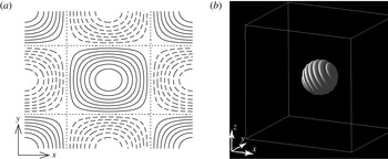
in incompressible viscous flow (figure 1
a). It is an exact solution of the Navier–Stokes equations even when the Reynolds number is finite if we allow
 $A$
to change in time. It is subject to a three-dimensional short-wave instability called elliptic instability (Sipp & Jacquin Reference Sipp and Jacquin1998; Kerswell Reference Kerswell2002). Small amplitude disturbances in the form of localized wave packets are superimposed to trigger the instability as in Hattori & bin Marzuki (Reference Hattori and bin Marzuki2014) (figure 1
b)
 $$\begin{eqnarray}\displaystyle \boldsymbol{u}^{\prime }=\boldsymbol{{\rm\nabla}}\times \boldsymbol{A},\quad \boldsymbol{A}=\boldsymbol{A}_{0}\text{e}^{-|\boldsymbol{x}|^{2}/r_{0}^{2}}\cos (\boldsymbol{k}_{0}\boldsymbol{\cdot }\boldsymbol{x}),\,\boldsymbol{k}_{0}=k_{0}[\sin {\it\chi},0,\cos {\it\chi}]^{\text{T}}. & & \displaystyle\end{eqnarray}$$
The direction of the wavevector
 $\boldsymbol{k}_{0}$
is set to the resonance angle of the elliptic instability at the origin:
 ${\it\chi}={\rm\pi}/3$
. These settings are ideal for the present purpose because periodic boundary conditions can be imposed in all three directions so that the Fourier spectral method, which gives sufficiently high precision, is used to solve the three-dimensional Navier–Stokes equations. The number of Fourier modes is
 $1024\times 1024\times 512$
in a unit cube
 $[-{\rm\pi},{\rm\pi}]\times [-L_{y}/2,L_{y}/2]\times [0,{\rm\pi}]$
, where
 $L_{y}=2{\rm\pi}/{\it\alpha}$
. In each unit cube there are four vortices, two of which have positive circulation while the other two have negative circulation, divided by the planes
 $x=(m+1/2){\rm\pi}$
and
 $y=(n+1/2)(L_{y}/2)$
, where
 $m$
and
 $n$
are integers. We would like to focus on the dynamics of a single vortex confined in a cell bounded by these planes. To this end symmetry with respect to the dividing planes, which is conserved with time evolution, is imposed on the initial conditions (Lundgren & Mansour Reference Lundgren and Mansour1996; Sipp & Jacquin Reference Sipp and Jacquin1998). Then the dividing planes or cell boundaries are unperturbed so that no fluid particle can move to a different cell. This does not imply that any flux through the cell boundaries vanishes; the magnitude of circulation in each cell decays as vorticity leaks out at the cell boundaries due to viscous flux. The interaction between neighbouring main vortices is suppressed, although thin vortex tubes interact strongly with their counterparts near the cell boundaries.
(a) Streamlines of two-dimensional flattened Taylor–Green vortices. (b) Initial localized disturbance. Iso-surface of the magnitude of vorticity.
 $|\boldsymbol{{\it\omega}}^{\prime }|=2.75{\it\omega}_{rms}^{\prime }$
, where
 ${\it\omega}_{rms}^{\prime }$
(
 $=7.771\times 10^{-3}$
at
 $t=0$
) is the root mean square of
 $|\boldsymbol{{\it\omega}}^{\prime }|$
.

For the parameter values of the base flow we set
 $A=2$
and
 ${\it\alpha}=\sqrt{1.5}$
, which gives the strain rate at the origin or elliptic stagnation point
 ${\it\epsilon}/A=0.1$
. The parameter values of the disturbance are chosen as
 $k_{0}=20,r_{0}={\rm\pi}/10,\boldsymbol{A}_{0}\propto [1/2,0,-\sqrt{3}/2]$
, while the magnitude of
 $\boldsymbol{A}_{0}$
is specified so that the ratio of the energy of the disturbance to that of the base flow is
 $3.16\times 10^{-7}$
. The Reynolds number based on the circulation in a single cell is
 $Re_{{\it\Gamma}}=1.31\times 10^{5}$
, while a case of lower Reynolds number
 $Re_{{\it\Gamma}}=6.53\times 10^{4}$
is also shown for comparison in figure 5. The resolution is sufficiently fine to capture the small scale of turbulence as
 $k_{max}{\it\eta}>1.91$
is large enough throughout the simulation, where
 $k_{max}\approx 482$
is the highest effective wavenumber and
 ${\it\eta}$
is the Kolmogorov scale. In the following the time scale is chosen so that the time period of rotation at the elliptic stagnation points is approximately equal to
 $2{\rm\pi}$
(exactly
 $2{\rm\pi}$
if
 ${\it\epsilon}/A$
were zero).
3 Results
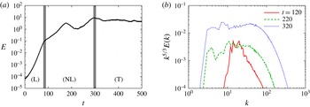
Time evolutions of the energy of the disturbance and its spectrum are shown in figure 2. The total velocity field is decomposed into the mean field
 $\boldsymbol{u}_{m}$
and the disturbance fields
 $\boldsymbol{u}^{\prime }$
as in Hattori & bin Marzuki (Reference Hattori and bin Marzuki2014)
 $$\begin{eqnarray}\displaystyle \boldsymbol{u}=\boldsymbol{u}_{m}+\boldsymbol{u}^{\prime },\quad \boldsymbol{u}_{m}=\mathop{\sum }_{\boldsymbol{k},k_{z}=0}\tilde{\boldsymbol{u}}_{\boldsymbol{k}}\text{e}^{\text{i}\boldsymbol{k}\boldsymbol{\cdot }\boldsymbol{x}},\,\boldsymbol{u}^{\prime }=\mathop{\sum }_{\boldsymbol{k},k_{z}\neq 0}\tilde{\boldsymbol{u}}_{\boldsymbol{k}}\text{e}^{\text{i}\boldsymbol{k}\boldsymbol{\cdot }\boldsymbol{x}}, & & \displaystyle\end{eqnarray}$$
where
 $\tilde{\boldsymbol{u}}_{\boldsymbol{k}}$
is the Fourier coefficient of the velocity field. The time evolution of the disturbance can be divided into three stages: linear, nonlinear and turbulent. In the linear stage
 $0\leqslant t\lesssim 80$
the energy of the disturbance grows exponentially due to the elliptic instability. The averaged growth rate in
 $60\leqslant t\leqslant 70$
is
 $0.117$
, which is smaller than the inviscid short-wave limit
 $2{\it\epsilon}(9/16)=0.225$
(Waleffe Reference Waleffe1990), mostly due to viscous effects. In the nonlinear stage
 $80\lesssim t\lesssim 300$
energy grows exponentially with reduced rate of growth for a while; it decreases after
 $t\approx 180$
and then increases again after
 $t\approx 220$
. Finally in the turbulent stage
 $300\lesssim t$
the energy spectrum of disturbance exhibits the
 $k^{-5/3}$
Kolmogorov scaling (figure 2
b), although the turbulent statistics is anisotropic owing to strong mean flow.
Time evolution of disturbance: (a) energy, (b) energy spectrum multiplied by
 $k^{5/3}$
. In (a) the linear, nonlinear and turbulent stages are marked by (L), (NL) and (T), respectively.

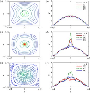
Figure 3 shows that the concentration of vorticity in the mean flow occurs in the latter half of the nonlinear stage. Here the time-averaged mean flow is obtained by taking the average of the
 $z$
component of the mean flow vorticity
 ${\it\omega}_{m,z}$
over a time period
 $t\leqslant t^{\prime }\leqslant t+10$
:
 $\overline{{\it\omega}}=(1/10)\int _{t}^{t+10}\,\text{d}t^{\prime }{\it\omega}_{m,z}$
. When
 $t\leqslant 160$
the mean flow is close to the base flow (figure 3
a,b). At
 $t=220$
a sharp peak appears at the origin (figure 3
c). This peak starts growing at
 $t\approx 200$
keeping its shape for
 $210\lesssim t\lesssim 240$
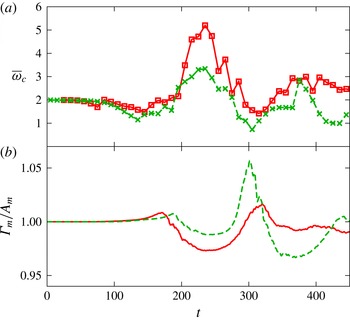
. The maximum of the averaged vorticity is 5.2, which is 2.6 times larger than the initial value, as shown later in figure 5. The peak decays after
 $t\approx 250$
. In the turbulent stage small-scale fluctuations are observed in the mean flow (figure 3
e). A peak of
 $\overline{{\it\omega}}\approx 3$
appears during the turbulent stage for
 $360\lesssim t\lesssim 400$
(figure 3
f), although it is smaller and wider than that in the nonlinear stage since energy or angular momentum decays faster because of turbulent dissipation.
Time evolution of mean flow averaged over
 $t\leqslant t^{\prime }\leqslant t+10$
. (a,c,e) Contours of vorticity, (b,d,f) vorticity distribution at
 $y=0$
. (a)
 $t=120$
, (c)
 $t=220$
, (e)
 $t=320$
.

The concentration of vorticity is closely related to selective decay of inviscid invariants
 $$\begin{eqnarray}\displaystyle & \displaystyle \text{circulation}\quad {\it\Gamma}=\int _{C_{z_{0}}}{\it\omega}_{z}\,\text{d}x\,\text{d}y, & \displaystyle\end{eqnarray}$$
 $$\begin{eqnarray}\displaystyle & \displaystyle \text{angular momentum}\quad A=\int _{V}h_{z}\,\text{d}x\,\text{d}y\,\text{d}z, & \displaystyle\end{eqnarray}$$
 $$\begin{eqnarray}\displaystyle & \displaystyle \text{energy}\quad E=\frac{1}{2}\int _{V}|\boldsymbol{u}|^{2}\,\text{d}x\,\text{d}y\,\text{d}z, & \displaystyle\end{eqnarray}$$
 $\boldsymbol{h}=\boldsymbol{r}\times \boldsymbol{u}$
,
 $V$
is the single cell
 $V=[-{\rm\pi}/2,{\rm\pi}/2]\times [-L_{y}/4,L_{y}/4]\times [0,{\rm\pi}]$
and
 $C_{z_{0}}$
is any section of the single cell
 $V$
perpendicular to the
 $z$
axis (
 $z=z_{0}$
). We calculate the above inviscid invariants for the mean flow
 $\boldsymbol{u}_{m}$
 $$\begin{eqnarray}\displaystyle & \displaystyle {\it\Gamma}_{m}=\int _{C_{0}}{\it\omega}_{m,z}\,\text{d}x\,\text{d}y, & \displaystyle\end{eqnarray}$$
 $$\begin{eqnarray}\displaystyle & \displaystyle A_{m}=\int _{C_{0}}h_{m,z}\,\text{d}x\,\text{d}y, & \displaystyle\end{eqnarray}$$
 $$\begin{eqnarray}\displaystyle & \displaystyle E_{m}=\frac{1}{2}\int _{C_{0}}|\boldsymbol{u}_{m}|^{2}\,\text{d}x\,\text{d}y. & \displaystyle\end{eqnarray}$$
 $C_{0}$
for all three quantities since the mean flow does not depend on
 $z$
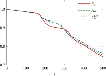
. Figure 4 shows time evolution of the three invariants calculated with the mean flow, where
 $E_{m}^{1/2}$
instead of
 $E_{m}$
is shown so that the three curves collapse in the linear stage. The rate of decay of circulation becomes large for
 $170\lesssim t\lesssim 210$
; it decays faster than the other two invariants. Then for
 $270\lesssim t\lesssim 310$
the rates of decay of the angular momentum and energy become large as the flow becomes fully turbulent (figure 2
b) so that energy dissipation becomes large, while the circulation decays rapidly again for
 $320\lesssim t\lesssim 360$
. Throughout the simulation the time evolutions of
 $A_{m}$
and
 $E_{m}^{1/2}$
are similar. Thus selective decay occurs for
 $170\lesssim t\lesssim 210$
, while weak selective decay also occurs for
 $320\lesssim t\lesssim 360$
.
Time evolution of circulation
 ${\it\Gamma}_{m}$
, angular momentum
 $A_{m}$
and square root of energy
 $E_{m}^{1/2}$
of mean flow. The values are normalized by the corresponding initial values.

Time evolution of (a) the averaged mean vorticity at the origin and (b) the ratio of circulation to angular momentum
 ${\it\Gamma}_{m}/A_{m}$
normalized by the initial value. Solid lines and squares:
 $Re_{{\it\Gamma}}=1.31\times 10^{5}$
, dashed lines and crosses:
 $Re_{{\it\Gamma}}=6.53\times 10^{4}$
.

How selective decay leads to concentration of vorticity is explained by a simple axisymmetric model. Let us consider an axisymmetric vortex in a circle of radius
 $r_{0}$
. Then the circulation is
 ${\it\Gamma}=2{\rm\pi}\int _{0}^{r_{0}}r{\it\omega}\,\text{d}r=r_{0}u_{{\it\theta}}(r_{0})$
, where
 $r$
is the distance from the axis of symmetry and
 $u_{{\it\theta}}$
is the azimuthal velocity, while
 $A=2{\rm\pi}\int _{0}^{r_{0}}r^{2}u_{{\it\theta}}\,\text{d}r$
. It would be legitimate to measure the core size
 $r_{c}$
of the vortex by
 $r_{c}^{2}=\int _{0}^{r_{0}}r^{3}{\it\omega}\,\text{d}r/\int _{0}^{r_{0}}r{\it\omega}\,\text{d}r$
, which can be expressed as
 $$\begin{eqnarray}\displaystyle r_{c}^{2}=r_{0}^{2}-\frac{2A}{{\it\Gamma}}. & & \displaystyle\end{eqnarray}$$
Thus when
 ${\it\Gamma}/A$
decreases, or in other words, circulation decays faster than angular momentum, the core size decreases leading to concentration of vorticity. Figure 5 confirms the above explanation. The time-averaged mean vorticity at the origin,
 $\overline{{\it\omega}}_{c}=\overline{{\it\omega}}(0,0)$
, increases (decreases) when
 ${\it\Gamma}_{m}/A_{m}$
decreases (increases). There are small fluctuations in
 $\overline{{\it\omega}}_{c}$
since the instantaneous vorticity field contains thin vortex tubes which move and interact with each other significantly (figure 6). The rapid decrease of
 ${\it\Gamma}_{m}/A_{m}$
in
 $300\leqslant t\leqslant 340$
for
 $Re_{{\it\Gamma}}=6.53\times 10^{4}$
gives only
 $\overline{{\it\omega}}_{c}\approx 3$
at
 $t\approx 370$
, which is smaller than
 $\overline{{\it\omega}}_{c}=5.2$
at
 $t\approx 230$
for
 $Re_{{\it\Gamma}}=1.31\times 10^{5}$
, since viscous diffusion is significant at the later time and the lower Reynolds number.
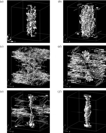
Iso-surface of the magnitude of vorticity.
 $|\boldsymbol{{\it\omega}}|=2.75{\it\omega}_{rms}$
, where
 ${\it\omega}_{rms}$
is the root mean square of
 $|\boldsymbol{{\it\omega}}|$
.
 $(t,{\it\omega}_{rms})=$
(a)
 $(120,1.224)$
, (b)
 $(160,2.559)$
, (c)
 $(180,7.095)$
, (d)
 $(200,4.006)$
, (e)
 $(220,1.745)$
, (f)
 $(240,1.334)$
.

What happens during selective decay can be understood by figure 6 which shows the iso-surface of the magnitude of vorticity. At
 $t=120$
, just after entering the nonlinear stage, blobs of strong vorticity are observed in a region near the
 $z$
axis or the centre of the original vortex (figure 6
a). The region expands at
 $t=160$
while some blobs are elongated by differential rotation of the mean flow to wrap around it (figure 6
b). At
 $t=180$
, just after the energy of the disturbance saturates, the number of blobs increases and they evolve into thin vortex tubes moving to the cell boundaries (figure 6
c). As time proceeds (
 $t=200$
and 220) the vortex tubes, which form pairs with their counterparts in the neighbouring cells, reconnect and eventually annihilate due to viscous diffusion at the cell boundaries following the process observed in Kerr (Reference Kerr2013) (figure 6
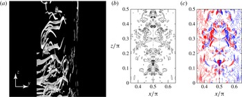
d,e). Although these vortex tubes look nearly horizontal after being stretched by the shearing motion of differential rotation, they are in general tilted (figure 7
a) and have net positive component of
 ${\it\omega}_{z}$
. Figure 7(b) shows the magnitude of vorticity
 $|\boldsymbol{{\it\omega}}|$
at
 $y=0$
; the dot-dashed line corresponds to the cell boundary
 $x={\rm\pi}/2$
, the left side (
 $x<{\rm\pi}/2$
) being the cell under consideration. Figure 7(c) shows that most of the vortex tubes, of which cross-sections are shown in figure 7(b), have the positive component of
 ${\it\omega}_{z}$
on the left side (
 $x<{\rm\pi}/2$
) of the cell boundary. The situation is reversed in the neighbouring cell on the right side (
 $x>{\rm\pi}/2$
), where the initial vortex has negative vorticity in the
 $z$
direction and the vortex tubes have a net negative component of
 ${\it\omega}_{z}$
. Therefore circulation decays as the vortex tubes reconnect and annihilate. Note that there is no significant change of angular momentum or energy in the reconnection and annihilation of the vortex tubes as shown in § 4.1. Hence selective decay. Finally at
 $t=240$
a vortex of smaller core size than that of the initial vortex is formed, while the thin vortex tubes disappear (figure 6
f).
(a) Iso-surface of the magnitude of vorticity. Magnified view near the cell boundary. The
 $z$
coordinates are five times larger than the
 $y$
coordinates.
 $(t,{\it\omega}_{rms})=(190,5.865)$
. (b) Contours of the magnitude of vorticity at
 $y=0$
at
 $t=190$
. The dot-dashed line is the cross-section of the cell boundary
 $x={\rm\pi}/2$
. The region is
 $0.35{\rm\pi}\leqslant x\leqslant 0.65{\rm\pi}$
and
 $0\leqslant z\leqslant {\rm\pi}/2$
. The increment of the contour levels is
 $0.5{\it\omega}_{rms}$
. (c) Contours of
 ${\it\omega}_{z}$
at
 $y=0$
at
 $t=190$
. The region is the same as in (b). The increment of the contour levels is
 $0.1{\it\omega}_{rms}$
. Red:
 ${\it\omega}_{z}>0$
, blue:
 ${\it\omega}_{z}<0$
.

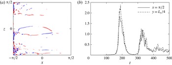
When vortex pairs reconnect at the cell boundaries, a vorticity component normal to the boundary should appear (Kida, Takaoka & Hussain Reference Kida, Takaoka and Hussain1991). Figure 8(a) shows the distribution of the normal component of vorticity
 ${\it\omega}_{y}$
at the cell boundary
 $y=L_{y}/4$
at
 $t=192$
when selective decay occurs. Positive (red) and negative (blue) regions of the vorticity component appear as a result of reconnection. They emerge as thin filamental regions and are convected to the left because of the flow field at the cell boundary. Consequently the regions are attracted to the neighbouring cell boundary
 $x=-{\rm\pi}/2$
and eventually annihilate. Figure 8(b) shows the time evolutions of
 $\int |{\it\omega}_{x}|\,\text{d}y\,\text{d}z$
at the cell boundary
 $x={\rm\pi}/2$
and
 $\int |{\it\omega}_{y}|\,\text{d}x\,\text{d}z$
at the cell boundary
 $y=L_{y}/4$
, which measure the activity of vortex reconnection. They become large when the decay rate of circulation is large (figure 4), confirming that the loss of circulation is due to the reconnection and annihilation of the vortex tubes.
(a) Distribution of
 ${\it\omega}_{y}$
at the cell boundary
 $y=L_{y}/4$
.
 $t=192$
. Red:
 ${\it\omega}_{y}>2$
, blue:
 ${\it\omega}_{y}<-2$
. (b) Time evolutions of
 $\int |{\it\omega}_{x}|\,\text{d}y\,\text{d}z$
at the cell boundary
 $x={\rm\pi}/2$
and
 $\int |{\it\omega}_{y}|\,\text{d}x\,\text{d}z$
at the cell boundary
 $y=L_{y}/4$
.

4 Discussion
4.1 How does the reconnection and annihilation of vortex pairs lead to selective decay?
In this section we show how the reconnection and subsequent annihilation of vortex pairs leads to selective decay. The key point is that vortices near the cell boundary have negligible contribution to angular momentum, while the contribution to circulation is constant inside the cell. In order to show this, we derive an expression of the angular momentum in terms of vorticity. In general we have
 $$\begin{eqnarray}\displaystyle \int _{D}\boldsymbol{r}\times \boldsymbol{u}\,\text{d}V=-\frac{1}{2}\int _{D}r^{2}\boldsymbol{{\it\omega}}\,\text{d}V+\frac{1}{2}\int _{\partial D}r^{2}(\boldsymbol{n}\times \boldsymbol{u})\,\text{d}S, & & \displaystyle\end{eqnarray}$$
where
 $D$
is the flow domain and
 $\boldsymbol{n}$
is the outward unit normal vector (Saffman Reference Saffman1992). We assume that
 $D$
is a circular cylinder of radius
 $r_{0}$
and the flow does not depend on the axial coordinate
 $z$
like mean flow:
 $\boldsymbol{u}=\boldsymbol{u}(x,y)$
. Then
 $$\begin{eqnarray}\displaystyle A & = & \displaystyle -\frac{1}{2}\int _{C}r^{2}{\it\omega}_{z}\,\text{d}x\,\text{d}y+\frac{r_{0}^{2}}{2}\oint _{\partial C}\boldsymbol{u}\boldsymbol{\cdot }\,\text{d}\boldsymbol{l}\nonumber\\ \displaystyle & = & \displaystyle -\frac{1}{2}\int _{C}r^{2}{\it\omega}_{z}\,\text{d}x\,\text{d}y+\frac{r_{0}^{2}}{2}\int _{C}{\it\omega}_{z}\,\text{d}x\,\text{d}y\nonumber\\ \displaystyle & = & \displaystyle \frac{1}{2}\int _{C}\left(r_{0}^{2}-r^{2}\right){\it\omega}_{z}\,\text{d}x\,\text{d}y,\end{eqnarray}$$
where the circle
 $C$
is a section of
 $D$
. Hence the weight function of the angular momentum is
 $w_{A}=(1/2)(r_{0}^{2}-r^{2})$
, which is monotonically decreasing in
 $r$
and vanishes at the boundary. It is also illuminating to see a simpler derivation of the weight function for the axisymmetric case
 $$\begin{eqnarray}\displaystyle A & = & \displaystyle \int _{0}^{r_{0}}ru_{{\it\theta}}(r)~r\,\text{d}r\nonumber\\ \displaystyle & = & \displaystyle \int _{0}^{r_{0}}\left(\int _{0}^{r}r^{\prime }{\it\omega}(r^{\prime })\,\text{d}r^{\prime }\right)r\,\text{d}r\nonumber\\ \displaystyle & = & \displaystyle \int _{0}^{r_{0}}\left(\int _{r^{\prime }}^{r_{0}}r\,\text{d}r\right){\it\omega}(r^{\prime })r^{\prime }\,\text{d}r^{\prime }\nonumber\\ \displaystyle & = & \displaystyle \frac{1}{2}\int _{0}^{r_{0}}(r_{0}^{2}-{r^{\prime }}^{2}){\it\omega}(r^{\prime })r^{\prime }\,\text{d}r^{\prime }.\end{eqnarray}$$
The above derivation shows that vorticity near the origin contributes to the azimuthal or rotational component of the flow everywhere in the domain, while vorticity near the boundary makes a negligible contribution to it. This implies that the vorticity near the boundary does not contribute to the total angular momentum very much. On the other hand, vorticity has a uniform contribution to the circulation. Therefore, when vorticity is transported to the boundary by a nearly inviscid process which conserves inviscid invariants and is lost at the boundary by reconnection or annihilation, circulation is lost while angular momentum is nearly unchanged for small viscosity.
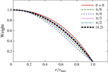
In the derivation of the weight function above it is essential that the domain is a circular cylinder. In the present case, the unit flow domain is a rectangular cell so that the weight function differs from that of (4.2). However, it can be evaluated numerically
 $$\begin{eqnarray}\displaystyle w_{A}(\boldsymbol{x}^{\prime })=\frac{{\rm\Delta}A}{{\rm\Delta}{\it\omega}}, & & \displaystyle\end{eqnarray}$$
where
 $$\begin{eqnarray}\displaystyle {\rm\Delta}A=A[{\it\omega}_{0}(\boldsymbol{x})+{\rm\Delta}{\it\omega}{\it\delta}(\boldsymbol{x}-\boldsymbol{x}^{\prime })]-A[{\it\omega}_{0}(\boldsymbol{x})], & & \displaystyle\end{eqnarray}$$
and
 $A[{\it\omega}(\boldsymbol{x})]$
denotes the value of the angular momentum for vorticity distribution
 ${\it\omega}(\boldsymbol{x})$
. Figure 9 shows the weight function evaluated for the unperturbed base flow of two-dimensional Taylor–Green vortices as
 ${\it\omega}_{0}$
by approximating the delta function in (4.5) by a Gaussian distribution of small width. It is seen that the weight function is not far from that of (4.2); more importantly, it vanishes at the boundary in all directions. Therefore, the discussion above holds true for the present case.
Weight function of angular momentum evaluated numerically for the base flow. It is evaluated along straight lines
 $y=(\tan {\it\theta})x$
.
 $r=(x^{2}+y^{2})^{1/2}$
is the distance from the origin and
 $r/r_{max}=1$
corresponds to the cell boundary. The value of weight function is normalized by the value at the origin. The thick dashed line shows (4.2). The thin lines show numerical results:
 ${\it\theta}=0$
(solid line),
 ${\rm\pi}/6$
(dashed line),
 ${\rm\pi}/4$
(dotted line),
 ${\rm\pi}/3$
(fine dotted line) and
 ${\rm\pi}/2$
(dot-dashed line).

4.2 Relevance to previous experiments and general applicability of the present results
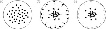
The essential mechanism of concentration of vorticity is depicted in figure 10. In this figure the vorticity of the mean flow is represented by point vortices of constant circulation shown by black circles. The shape of the region can be arbitrary; a circle is chosen for simplicity. Initially the vortices are distributed loosely (figure 10 a). Some of them approach the boundary as thin vortex tubes move to the cell boundaries as shown in figures 6(c) and 6(d). Then the rest of the vortices get close to the origin to keep the angular momentum unchanged (figure 10 b). Finally the vortices annihilate at the boundary and vorticity concentrates near the origin (figure 10 c).
Schematic diagram of concentration of vorticity. Vorticity of the mean flow is represented by point vortices shown by black circles. (a) Initial state, (b) some vortices approach the boundary, (c) vortices annihilate at the boundary.

The above scenario may look oversimplified. However, it elucidates the key ingredients of selective decay: (i) angular momentum is approximately conserved; and (ii) circulation is lost at the boundary. It also gives a clue to discussions of the applicability of the mechanism to more general cases.
First, vorticity should be convected to the boundary (figure 10 b). In the present study thin vortex tubes appear as a result of elliptic instability; a localized disturbance, which is a sum of inertial waves, is amplified by the elliptic instability. It is worth noting that the ‘combined action of inertial wave motion and turbulence’ is regarded to lead to concentration of vorticity in McEwan (Reference McEwan1973). We have chosen the elliptic instability to amplify a localized disturbance ‘naturally’, since we do not prefer external forcing which may create somewhat artificial disturbances. However, thin vortex tubes are created in many other flows. For example, thin vortex tubes were shown to emerge and wrap around an initially symmetric vortex in Melander & Hussain (Reference Melander and Hussain1993) and Takahashi, Ishii & Miyazaki (Reference Takahashi, Ishii and Miyazaki2005), who studied the interaction between a coherent vortex and external turbulence.
Next, we point out that reconnection and annihilation of vortex pairs are irreversible processes; once vortices come close to the boundary and start reconnection or annihilation with their counterparts across the boundary, they cannot leave the boundary. In this sense the boundary can be regarded as a ‘sink’ of vorticity of the mean flow. This is more or less true for other boundary conditions. The region need not be symmetric and can be quite general since reconnection of vortices occurs in asymmetric cases (Boratav, Pelz & Zabusky Reference Boratav, Pelz and Zabusky1992; Marshally, Brancher & Giovannini Reference Marshally, Brancher and Giovannini2001). Thus concentration of vorticity can occur when a coherent vortical structure with turbulent fluctuations comes close to another structure whose mean vorticity is of the opposite sign, forming a quasi-vortex pair. When the boundary is a rigid wall where no-slip conditions are imposed, as in the experiments by McEwan (Reference McEwan1973) and Hopfinger et al. (Reference Hopfinger, Browand and Gagne1982), boundary layers and resulting secondary vortices may affect the motion of the vortices; total circulation in the entire region is constant since the variation of the circulation of the main vortex is compensated by the vorticity in the boundary layer. However, if we consider the circulation outside the boundary layer instead of the total circulation, concentration of vorticity may occur following the above scenario. Concentration of vorticity observed in the previous experiments (McEwan Reference McEwan1973; Hopfinger et al. Reference Hopfinger, Browand and Gagne1982) may be explained by the present mechanism, although further careful argument should follow for accurate conclusions.
Our new finding is that the sink of vorticity due to the reconnection and annihilation of vortex pairs at the boundary, rather than bulk action of the Reynolds stress, is the driving force of concentration. The relation
 $r_{c}^{2}=r_{0}^{2}-2A/{\it\Gamma}$
tells us that the ratio
 ${\it\Gamma}/A$
should decrease in order for the vorticity to concentrate at the centre, unless the vorticity also concentrates at the boundary. Since both circulation
 ${\it\Gamma}$
and angular momentum
 $A$
change due to the flux at the boundary, concentration of vorticity is better understood by considering the boundary effect.
Concentration of vorticity is observed in a limited interval of the nonlinear stage, while weaker concentration is observed also at the turbulent stage. This is due to the settings which are ideal for ‘natural’ evolution of disturbances but inadequate for keeping the concentrated vortex alive for a sufficiently long time. We point out that the Reynolds number in the present study,
 $Re_{{\it\Gamma}}=1.31\times 10^{5}$
, is much smaller than those in the experiments (e.g.
 $Re_{{\it\Gamma}}\sim 2.4\times 10^{6}$
in McEwan (Reference McEwan1973)). Thus we should grow the disturbance before the system decays due to viscous and turbulent diffusion. As a result the nonlinear stage, at which concentration of vorticity occurs, cannot be sufficiently long. As the system enters the turbulent stage the energy and correspondingly the angular momentum of the mean flow start decaying rapidly (figure 4) and the sharp peak of concentrated vorticity is lost (figure 5). Concentration of vorticity is expected to survive as far as the system is at the nonlinear stage or weakly (not strongly) turbulent. The interval of the nonlinear stage can be extended for small
 ${\it\epsilon}$
and high Reynolds numbers or by input of energy; it would be quite long in some geophysical flows like rapidly rotating turbulence, where quasi-two-dimensional structures are dominant. In addition, concentration will be stronger for higher Reynolds numbers, as expected by comparing the results of the two Reynolds numbers (figure 5). Concentration of vorticity in these flows should be studied in future works, although computational costs would be high for these cases.
5 Concluding remarks
To summarize, we have shown that concentration of vorticity occurs in the two-dimensional flattened Taylor–Green vortices due to selective decay of inviscid invariants. Reconnection and subsequent annihilation of vortex pairs are responsible for the selective decay, as they decrease only circulation. Similar processes are expected to give rise to strong thin vortices in general when large-scale vortices with turbulent fluctuations come close to each other; this should be studied in future works. What happens in flows similar to previous experiments is also of interest. In this regard we point out that the elliptical flow confined in a rotating cylinder lost vorticity in the core to get close to a hollow vortex (Hattori & bin Marzuki Reference Hattori and bin Marzuki2014); in this case energy decayed significantly after transition to turbulence while circulation was constant, which implies
 $r_{c}^{2}$
should increase.
One may think that the mechanism of concentration of vorticity shown in the present paper is related to vorticity stripping (Legras & Dritschel Reference Legras and Dritschel1993), which also causes concentration of vorticity by throwing away weak vorticity. Although the value of vorticity cannot increase in the two-dimensional contour dynamics simulation by Legras & Dritschel (Reference Legras and Dritschel1993), it would be interesting to seek the relevance of their work to the present results.
Two more brief remarks should be given. First, vorticity does not concentrate if a normal mode of large wavelength is used as a disturbance instead of the localized disturbance. In this case the normal mode keeps growing exponentially until a nonlinear process suddenly collapses the vortex so that all three invariants decrease simultaneously. Next, the shape of the peak in the vorticity of the mean flow cannot be predicted by selective decay only. Further assumptions should be made to evaluate the height and width of the peak.
Acknowledgements
This work was supported by JSPS KAKENHI grant number 24540391. Numerical calculations were performed on SGI UV1000 and UV2000 at the Institute of Fluid Science, Tohoku University.