1. Introduction
Spatially accelerating flows are present in a wide range of applications in engineering and the natural sciences, ranging from aerofoils and turbine blades to atmospheric flows over a complex landscape. Although the kinetic energy of the mean flow increases as a result of the acceleration, turbulence may become less vigorous and the flow may revert to a quasi-laminar state, through a process called ‘relaminarization’ or, more accurately, ‘quasi-laminarization’. Various parameters are used to quantify the acceleration level; one of the most widely used is the acceleration parameter,
 $K=({\it\nu}/U_{\infty }^{2})\,\text{d}U_{\infty }/\text{d}x$
, where
 $x$
is the streamwise direction,
 $U_{\infty }$
is the free-stream velocity in this direction and
 ${\it\nu}$
is the kinematic viscosity. In sink flows (the equilibrium accelerating boundary layer that occurs in a long converging duct with straight walls), Spalart (Reference Spalart1986) showed that turbulence cannot be sustained if
 $K$
is higher than a critical value of
 $2.5{-}3.0\times 10^{-6}$
.
The mechanisms of quasi-laminarization have been widely studied. Narasimha & Sreenivasan (Reference Narasimha and Sreenivasan1973) attributed the reversion to the dominance of pressure forces over the slowly responding Reynolds stresses in an originally turbulent flow, which leads to the generation of a new laminar boundary layer stabilized by the favourable pressure gradient (FPG). Although the turbulence does not decrease in the region of strong acceleration, it plays an increasingly passive role in the development of the boundary layer (Launder Reference Launder1964). The production of turbulence was found to exceed dissipation in the quasi-laminar region (Narasimha & Sreenivasan Reference Narasimha and Sreenivasan1973), indicating that the reversion is not a pure Reynolds-number effect.
The quasi-laminarization has been found to be associated with a decrease of bursting frequency and stabilization of the near-wall turbulent structures. McEligot & Eckelmann (Reference McEligot and Eckelmann2006) observed that the burst frequency is very sensitive to the acceleration, decreasing as
 $K$
increases; the intensity of the wall-normal fluctuations also decreases, leading to weaker momentum transport.
Bourassa & Thomas (Reference Bourassa and Thomas2009) related quasi-laminarization to the stabilizing effects of acceleration on near-wall streaky structures caused by the decrease of the wall-normal and spanwise fluctuations, which are responsible for the instability of streaks and near-wall vortices (Jiménez & Pinelli Reference Jiménez and Pinelli1999; Schoppa & Hussain Reference Schoppa and Hussain2002). Furthermore, quadrant analysis (Wallace, Eckelmann & Brodkey Reference Wallace, Eckelmann and Brodkey1973) showed that a weaker inner–outer-layer interaction results from a decrease of both sweeps (Quadrant 4, Q4, events) and ejections (Q2 events): Q4 events are eliminated and alias to third-quadrant (inward interaction) events due to the acceleration, and Q2 events become more intermittent, due to the increased spanwise separation of streaks. Joshi, Liu & Katz (Reference Joshi, Liu and Katz2014) related quasi-laminarization to a decrease of Q2 events that is believed to be associated with sweeping events and local regions of adverse pressure gradient, which are eliminated by the strong favourable mean pressure gradients.
Recent numerical simulations by Piomelli & Yuan (Reference Piomelli and Yuan2013) showed that the damping of wall-normal and spanwise turbulent fluctuations is due to the decrease of the magnitude of the pressure fluctuations, which is caused by a decrease of the source term of the Poisson equation for the rapid component of the pressure fluctuations. This lessens the redistribution of turbulent kinetic energy (TKE) into wall-normal and spanwise fluctuations, leading to quasi-one-dimensional turbulence in the quasi-laminarization zone. Intensifying the wall-normal and spanwise fluctuations by introducing wall roughness, on the other hand, leads to strongly destabilized near-wall structures, and either a complete lack of quasi-laminarization or an early re-establishment of the equilibrium turbulent flow, depending on the roughness height. The results suggest that the near-wall region has an important effect on the quasi-laminarization process.
Roughness is known to play a major role in the dynamics of near-wall turbulence, and a substantial amount of work has been carried out to understand the dynamics of turbulent flows over rough walls, for both engineering and environmental applications, summarized in Raupach, Antonia & Rajagopalan (Reference Raupach, Antonia and Rajagopalan1991) and Jiménez (Reference Jiménez2004). Roughness increases the drag on the wall due to the pressure drag resulting from the wake created downstream of a roughness element. Many studies (e.g. Flack, Schultz & Shapiro Reference Flack, Schultz and Shapiro2005) have shown that, far away from the wall, roughness does not affect the turbulence statistics, but only sets the velocity scale at the wall. In addition, near the rough wall the TKE is more homogeneously distributed in the three directions, and the turbulent structures are clearly altered.
Although most of the experimental and numerical work has concentrated on canonical pipe, channel flows or boundary layers, several studies have addressed the interaction of roughness with the favourable pressure gradient. Coleman, Moffat & Kays (Reference Coleman, Moffat and Kays1977) measured the velocity field in a rough-wall accelerating boundary layer in a quasi-equilibrium state, where the velocity achieved self-similarity and the Reynolds number and accelerating parameter were constant, but the exact equilibrium behaviour (Rotta Reference Rotta1962) was not satisfied. A favourable pressure gradient was found to make the surface ‘rougher’ by increasing the friction velocity,
 $u_{{\it\tau}}$
; the increase of
 $u_{{\it\tau}}$
was faster than that of
 $U_{\infty }$
, producing a higher friction coefficient,
 $C_{f}=2(u_{{\it\tau}}/U_{\infty })^{2}$
. The turbulent kinetic energy decreased when normalized using
 $U_{\infty }$
, especially its wall-normal and spanwise components, while the streamwise component was unchanged, leading to higher anisotropy. Tachie and co-workers (Tachie, Agelin-Chaab & Shah Reference Tachie, Agelin-Chaab and Shah2007; Tachie & Shah Reference Tachie and Shah2008) conducted experiments in flows over bar roughness under strong FPG achieved with converging side walls or an inclined bottom wall in open-channel flows. Contrary to the observation of Coleman et al. (Reference Coleman, Moffat and Kays1977), their data showed that
 $C_{f}$
, the mean-velocity defect, and the Reynolds stresses were largely independent of the pressure gradient. This was probably due to the limited streamwise distance for the FPG to exert its effects. Cal et al. (Reference Cal, Brzek, Johansson and Castillo2008, Reference Cal, Brzek, Johansson and Castillo2009) performed experimental studies in non-equilibrium boundary layers subjected to acceleration achieved using a tilted plane, with fairly mild acceleration (
 $K<0.5\times 10^{-6}$
). FPG leads to an increase of
 $C_{f}$
and a decrease of bulk Reynolds number. In the outer layer, competing effects of FPG and roughness were found on the mean flow and the Reynolds stresses; however, close to the rough wall, both roughness and acceleration intensify the fluctuations significantly, with the Reynolds-stress anisotropy unaffected by FPG; this was different from the observations of both Coleman et al. (Reference Coleman, Moffat and Kays1977) and Tachie & Shah (Reference Tachie and Shah2008). Similar observations on the opposite effects of FPG and roughness and the higher
 $C_{f}$
were also made from large-eddy simulations (LES) of spatially developing flows over roughness by Piomelli & Yuan (Reference Piomelli and Yuan2013).
The sink flow, on the other hand, exhibits a different behaviour. Yuan & Piomelli (Reference Yuan and Piomelli2014b
) showed that a stronger acceleration causes a decrease in
 $C_{f}$
, instead of promoting it as in the non-equilibrium accelerating flows. The opposite effects of FPG and roughness on the drag and turbulent intensities combine to influence the flow in a way that depends on the roughness Reynolds number,
 $k_{s}^{+}$
, where
 $k_{s}$
is the equivalent sandgrain height, defined as the mean height of the uniform sandgrain roughness (Nikuradse Reference Nikuradse1933) that produces the same drag as the roughness in question, and
 $+$
denotes quantities normalized by the friction velocity,
 $u_{{\it\tau}}$
, and
 ${\it\nu}$
. They found that flow reversion is achieved only when the flow is close to the hydraulically smooth regime, i.e. when the FPG is strong enough to overcome the roughness effects resulting in a low value of
 $k_{s}^{+}$
. In the outer layer, FPG effects always dominate those of roughness.
These results indicate that the effects of roughness and FPG are interdependent, and are affected by the state of the flow (equilibrium or not). Deeper understanding of the flow dynamics is required to explain how the two effects are related and manifested in different flow states. Moreover, the different results from previous studies of non-equilibrium flows with mild
 $K$
or a relatively short accelerating distance motivate the study of a non-equilibrium accelerating boundary with strong
 $K$
lasting for a sufficient distance for its effect to be significant. To this end, we carried out direct numerical simulations (DNS) of a spatially developing rough-wall boundary layer flow with free-stream acceleration, compared to a smooth-wall LES taken from case LES3s in Piomelli & Yuan (Reference Piomelli and Yuan2013). The problem set-up and numerical techniques are introduced in § 2. The developments in boundary layer (§ 3.1) and mean velocity (§ 3.2) are then presented. Then the time-averaged wake fluctuation and its statistics are discussed in § 3.3. Lastly, the turbulent statistics are shown in § 3.4 and the causes of the differences in Reynolds-stress anisotropy are studied in detail in § 3.5.
2. Problem formulation
The incompressible flow of a Newtonian fluid is governed by the equations of conservation of mass and momentum:
 $$\begin{eqnarray}\displaystyle & \displaystyle \frac{\partial u_{i}}{\partial x_{i}}=0, & \displaystyle\end{eqnarray}$$
 $$\begin{eqnarray}\displaystyle & \displaystyle \frac{\partial u_{i}}{\partial t}+\frac{\partial u_{i}u_{j}}{\partial x_{j}}=-\frac{\partial P}{\partial x_{i}}+{\it\nu}\frac{\partial ^{2}u_{i}}{\partial {x_{j}}^{2}}+F_{i}, & \displaystyle\end{eqnarray}$$
 $x_{1}$
,
 $x_{2}$
and
 $x_{3}$
(or
 $x$
,
 $y$
and
 $z$
) are, respectively, the streamwise, wall-normal and spanwise directions, and
 $u_{i}$
(or
 $u$
,
 $v$
and
 $w$
) are the velocity components in those directions;
 $P=p/{\it\rho}$
is the modified pressure, and
 ${\it\rho}$
the density. For the LES, (2.1)–(2.2) are solved for filtered quantities, and the divergence of the sub-grid stress tensor,
 ${\it\tau}_{ij}=\overline{u_{i}u_{j}}-\overline{u}_{i}\overline{u}_{j}$
, appears on the right-hand side of the momentum equation;
 ${\it\tau}_{ij}$
is modelled using a dynamic eddy–viscosity model (Germano et al.
Reference Germano, Piomelli, Moin and Cabot1991; Lilly Reference Lilly1992), in which the coefficient is adjusted using the Lagrangian-averaging procedure (Meneveau, Lund & Cabot Reference Meneveau, Lund and Cabot1996). The numerical simulations are performed using a well-validated code that solves (2.1) and (2.2) on a staggered grid using second-order, central differences for all terms, a second-order semi-implicit time advancement and MPI (message passing interface) parallelization (Keating et al.
Reference Keating, Piomelli, Bremhorst and Nešić2004). In the rough-wall studies, an immersed-boundary method (IBM) based on the volume-of-fluid approach (Yuan & Piomelli Reference Yuan and Piomelli2014b
) is used to impose the no-slip boundary condition on the rough surfaces. A body force,
 $F_{i}$
in the
 $x_{i}$
direction, results from the IBM; it is non-zero in the interface cell only. In the smooth-wall case,
 $F_{i}=0$
.
For both cases, the acceleration is achieved by imposing a spatially varying free-stream velocity in the streamwise direction,
 $U_{\infty }(x)$
; the vertical component,
 $V_{\infty }(x)$
, is calculated through mass balance; a no-slip boundary condition is applied at the bottom wall (or on the rough surface through IBM); the turbulent inflow at
 $x/{\it\delta}_{o}^{\ast }=0$
(reference plane) is generated from a rescaling/recycling region (Lund, Wu & Squires Reference Lund, Wu and Squires1998). Periodic boundary conditions are applied in the spanwise direction
 $z$
, and the convective outflow (Orlanski Reference Orlanski1976) is used at the domain outlet.
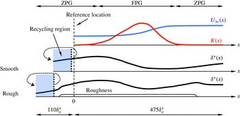
Sketch of the configurations for the smooth (Piomelli & Yuan Reference Piomelli and Yuan2013) and rough cases.

Figure 1 presents a sketch of the configuration. The long domain in
 $x$
allows the boundary layer to evolve for a sufficient distance (around
 $300{\it\delta}_{o}^{\ast }$
, where
 ${\it\delta}^{\ast }$
is the displacement thickness and the subscript ‘o’ denotes the reference plane) for the acceleration effects to develop; the spanwise domain size is sufficient to enclose the largest turbulent eddies in the outer layer; moreover,
 $L_{y}/{\it\delta}_{95}\geqslant 6$
(where
 ${\it\delta}_{95}$
, or
 ${\it\delta}$
, is the boundary-layer thickness) to avoid blockage effects. The domain size and
 ${\it\delta}$
in the rescaling region are adjusted so that, at
 $x=0$
, the rough-wall boundary layer matches (within 2 %) the local Reynolds number of the smooth case,
 $\mathit{Re}_{{\it\delta}^{\ast },o}=1240$
based on
 ${\it\delta}_{o}^{\ast }$
and
 $U_{\infty ,o}$
. The inlet Reynolds number and the
 $K(x)$
distribution are the same as Case 2 in the experimental studies of Warnack & Fernholz (Reference Warnack and Fernholz1998). Roughness starts at a location downstream of the recycling plane, while leaving a sufficient distance before the reference plane for the boundary layer to become well developed at
 $x/{\it\delta}_{o}^{\ast }=0$
. The present study is focused mainly on the FPG region (
 $50\lesssim x/{\it\delta}_{o}^{\ast }\lesssim 350$
).
The roughness is modelled as a dense distribution of randomly rotated ellipsoids (‘sandgrains’) with the same shape and size (Scotti Reference Scotti2006); the semi-axes of the ellipsoid are
 $k$
,
 $1.4k$
and
 $2k$
, where
 $k$
is the roughness height. This roughness model has been calibrated so that
 $k$
approximates
 $k_{s}$
in the transitionally rough regime. The fully rough regime starts at
 $k^{+}\approx 60$
; in this regime, the equivalent sandgrain height is a fixed value (denoted by
 $k_{s\infty }$
) and equals
 $1.6k$
(Yuan & Piomelli Reference Yuan and Piomelli2014a
) for the present roughness. As the free stream accelerates,
 $k^{+}$
increases from around 20–80, developing from the transitionally rough flow to a fully rough flow at
 $x/{\it\delta}_{o}^{\ast }\approx 220$
.
 ${\it\delta}$
is between 10 and 20 times larger than
 $k$
, with the lower limit reached only within a narrow band in the FPG region; these values are within the common range used in numerical simulations in the literature (Bhaganagar, Coleman & Kim Reference Bhaganagar, Coleman and Kim2007; Ikeda & Durbin Reference Ikeda and Durbin2007; Lee, Sung & Krogstad Reference Lee, Sung and Krogstad2011).
For the rough case,
 $10\leqslant {\rm\Delta}x^{+}\leqslant 21$
and
 $5\leqslant {\rm\Delta}z^{+}\leqslant 14$
; the coarser limit is reached only at the end of the FPG region due to the increased friction velocity. The present grid sizes in plus units are comparable to the values used in existing DNS studies on rough-wall boundary layers and channel flows. For examples, Castillo et al. (Reference Castillo, Chen, Araya, Newman, Jansen and Castillo2013) used
 ${\rm\Delta}x^{+}=23$
,
 ${\rm\Delta}z^{+}=11$
and
 ${\rm\Delta}y_{\mathit{min}}^{+}=0.5$
; in Ikeda & Durbin (Reference Ikeda and Durbin2007),
 ${\rm\Delta}x^{+}=12$
,
 ${\rm\Delta}z^{+}=11$
and
 ${\rm\Delta}y_{\mathit{min}}^{+}=0.4$
; similar sizes were also used in Coceal et al. (Reference Coceal, Thomas, Castro and Belcher2006), where
 ${\rm\Delta}x^{+}$
and
 ${\rm\Delta}z^{+}$
equal to 16 were considered sufficient. It was pointed out by Moin & Mahesh (Reference Moin and Mahesh1998) that a sufficient spatial resolution should capture most of the dissipation, which occurs for scales of
 $O({\it\eta})$
, where
 ${\it\eta}=({\it\nu}/{\it\epsilon})^{1/4}$
(
 ${\it\epsilon}$
is the dissipation rate of TKE) is the Kolmogorov length scale. For a curved channel flow, scales less than
 $15{\it\eta}$
contributed to most of the dissipation (Moser & Moin Reference Moser and Moin1987). The present resolution gives
 ${\rm\Delta}x/{\it\eta}\leqslant 10$
and
 ${\rm\Delta}z/{\it\eta}\leqslant 7$
. In addition, this resolution is capable of resolving the shape of roughness elements and the flow structures developed around them: from 5 to 8 grid points in
 $x$
and 10 points in
 $z$
are used to resolve each roughness element; 101 points in
 $y$
are used below the roughness crest. The resolution in the
 $x{-}z$
plane might be marginal for the element shape, but it is considered sufficient since the main purpose here is not to reproduce a particular geometry perfectly, but rather to introduce a perturbation on the wall capable of providing the form drag.
The total simulation time is
 $85{\it\delta}_{o}^{\ast }/u_{{\it\tau}}$
and
 $145{\it\delta}_{o}^{\ast }/u_{{\it\tau}}$
for the rough and smooth cases, respectively, sufficient to achieve convergence for second- and third-order turbulent statistics and Reynolds-stress budgets. A summary of simulation parameters is presented in table 1.
Simulation parameters (
 $L$
is the length of the computational domain).

For the smooth case, a flow quantity is decomposed into two components
 $$\begin{eqnarray}{\it\theta}(x,y,z,t)=\langle \overline{{\it\theta}}\rangle (x,y)+{\it\theta}^{\prime }(x,y,z,t),\end{eqnarray}$$
where
 $\langle {\it\theta}\rangle$
,
 $\overline{({\it\theta})}$
and
 ${\it\theta}^{\prime }$
are the spatial average, the temporal average and the turbulent fluctuation, respectively. For the rough case,
 ${\it\theta}$
also includes the wake component
 $\widetilde{{\it\theta}}$
, the spatial variation of the time-averaged field due to the spatial heterogeneity of the roughness geometry,
 $$\begin{eqnarray}{\it\theta}(x,y,z,t)=\langle \overline{{\it\theta}}\rangle (x,y)+\widetilde{{\it\theta}}(x,y,z)+{\it\theta}^{\prime }(x,y,z,t).\end{eqnarray}$$
 $\widetilde{{\it\theta}}$
is significant in the roughness sublayer only. In the smooth case the spatial averaging is performed in the spanwise direction only, while in the rough case the averaging is also carried out over
 $50k$
in the streamwise direction to compensate for the limited sampling of random roughness elements in the spanwise direction. The averaging length is large compared to the roughness scale, but small enough (1–10 %) compared to the acceleration length scale,
 $U_{\infty }(x)/(\text{d}U_{\infty }(x)/\text{d}x)$
, in the FPG region. Note that
 $\langle \cdot \rangle$
is obtained from the fluid domain only; it is also called the ‘intrinsic average’ (Nikora et al.
Reference Nikora, McEwan, McLean, Coleman, Pokrajac and Walters2007; Mignot, Bartheleemy & Hurther Reference Mignot, Bartheleemy and Hurther2009). In contrast, the averaging over both the solid and fluid domains is called the ‘superficial average’, denoted as
 $\langle \cdot \rangle _{s}$
.
3. Results
3.1. Boundary-layer development
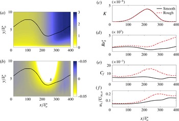
The contours of the streamwise and wall-normal mean velocities are shown in figure 2(a,b). In both cases, the boundary layer becomes thinner in the FPG region, with irrotational flow entrained into the boundary layer. The streamwise development of
 $\mathit{Re}_{{\it\delta}^{\ast }}$
and
 $C_{f}$
is shown in figure 2(d,e). The total drag, for the rough-wall case, is the sum of viscous and pressure components, and is calculated from the vertical integral of the IBM force (Yuan & Piomelli Reference Yuan and Piomelli2014b
). Acceleration causes a decrease of the local Reynolds number, as the boundary-layer thinning is faster than the increase of
 $U_{\infty }$
. This is more significant in the smooth case; on the rough wall, the dip in Reynolds number is much less significant.
Contours of (a)
 $\langle \overline{u}\rangle /U_{\infty ,o}$
and (b)
 $\langle \overline{v}\rangle /U_{\infty ,o}$
; ——
 ${\it\delta}$
. Boundary-layer integral parameters: (c) acceleration parameter
 $K$
; (d) Reynolds number
 $\mathit{Re}_{{\it\delta}^{\ast }}=U_{\infty }{\it\delta}^{\ast }/{\it\nu}$
, (e) friction coefficient,
 $C_{f}=2u_{{\it\tau}}^{2}/U_{\infty }^{2}$
and (f) friction velocity,
 $u_{{\it\tau}}/U_{\infty ,o}$
.
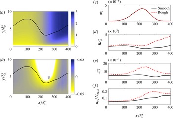
On the smooth wall, during the initial acceleration
 $C_{f}$
stays almost constant, as the wall shear stress adapts to the acceleration; in the region of quasi-laminarization,
 $250\lesssim x/{\it\delta}_{o}^{\ast }\lesssim 300$
, however,
 $u_{{\it\tau}}$
remains almost constant and
 $C_{f}$
exhibits a dip. The rough case, on the other hand, presents a significant increase of
 $C_{f}$
in the acceleration region, indicating that
 $u_{{\it\tau}}$
increases much faster than
 $U_{\infty }$
: the turbulent motions on the rough wall are not, in this case, attenuated by acceleration, but instead intensified.
To explain the variation of the rough wall
 $u_{{\it\tau}}$
, we consider the dependence of the drag (either the viscous or the form drag) on the velocity relative to the roughness element. The drag force exerted by each roughness element can be expressed as
 $$\begin{eqnarray}D\approx \frac{{\it\rho}}{2}\mathscr{U}(x)^{2}C_{D}A,\end{eqnarray}$$
where
 $A$
is the bed area covered by the element,
 $\mathscr{U}$
is the velocity outside the wake region, taken here as the velocity at the top of the roughness sublayer,
 $U_{RS}(x)=\langle \overline{u}\rangle (x,2k)$
and
 $C_{D}$
is the drag coefficient of the element, dependent on the element shape and, in transitionally rough flows, on the Reynolds number; for fully rough flows, however,
 $C_{D}$
is independent of the Reynolds number. For the flow above the roughness sublayer in an averaged sense, this amounts to a wall shear stress,
 ${\it\tau}_{w}={\it\rho}u_{{\it\tau}}^{2}$
, which is the density of the total drag per unit area,
 $$\begin{eqnarray}{\it\tau}_{w}(x)\approx \frac{{\it\rho}}{2}U_{RS}(x)^{2}\overline{C_{D}},\end{eqnarray}$$
where
 $\overline{C_{D}}$
is the drag coefficient averaged over all roughness elements. To verify this dependence of drag on
 $U_{RS}$
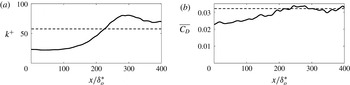
, figure 3 plots
 $\overline{C_{D}}=2{\it\tau}_{w}(x)/{\it\rho}U_{RS}(x)^{2}$
compared to
 $k_{s}^{+}(x)$
. The fully rough regime (
 $k^{+}\gtrsim 60$
) is achieved for
 $x/{\it\delta}_{o}^{\ast }\gtrsim 220$
(figure 3
a), where
 $\overline{C_{D}}$
becomes approximately constant (figure 3
b). This indicates that the increase of drag in the FPG region is due to the near-wall acceleration, caused by the acceleration of
 $U_{\infty }$
and the thinning of the boundary layer.
(a) Streamwise variation of the roughness Reynolds number; – – –
 $k^{+}=60$
. (b) Streamwise variation of
 $\overline{C_{D}}=2(u_{{\it\tau}}/U_{RS})^{2}$
; – – – the constant value (0.032) in the fully rough region (
 $220<x/{\it\delta}_{o}^{\ast }<400$
).

3.2. Mean velocity
The mean streamwise velocity
 $U=\langle \overline{u}\rangle$
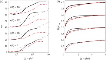
is shown in figure 4 for both cases. Here,
 $d$
is the zero-plane displacement, representing the effective elevation of the boundary layer due to roughness.
 $d$
is obtained as the location of the centroid of the wall-normal profile of the time- and space-averaged drag force, i.e. the location where the wall shear stress appears to act (Jackson Reference Jackson1981);
 $d\approx 0.8k$
, not noticeably affected by the FPG. Acceleration leads to a decrease of the slope of the logarithmic layer (a well-known property of accelerating boundary layers), and, in the smooth case, to a laminar-like mean flow in the quasi-laminar region (
 $x/{\it\delta}_{o}^{\ast }=300$
in figure 4
a), and a well-mixed region with weaker velocity gradient,
 $\partial U/\partial y$
, in the outer layer (figure 4
b). The universal logarithmic profile is restored after retransition, as shown at
 $x/{\it\delta}_{o}^{\ast }=400$
. Similarly, the rough-wall mean flow displays a decrease of logarithmic slope; however, figure 4(b) shows an earlier restoration of the slope to its initial value, before
 $x/{\it\delta}_{o}^{\ast }=300$
.
Profiles of mean streamwise velocity
 $U$
at various streamwise locations, normalized in (a) wall units and (b) outer scaling; —— smooth and – – – rough walls. The thin dashed lines in (a) indicate
 $u^{+}=y^{+}$
and the universal logarithmic law
 $u^{+}=\log y^{+}/0.40+5.0$
; the thin lines in (b) show the velocity profiles at the reference location
 $x/{\it\delta}_{o}^{\ast }=0$
.

The local values of the logarithmic slope and intercept are denoted as
 $\widetilde{{\it\kappa}}(x)$
and
 $\widetilde{B}(x)$
to distinguish them from the universal values for the canonical boundary layer (taken here as
 ${\it\kappa}=0.40$
and
 $B=5.0$
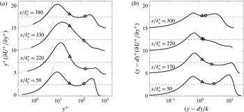
). Following Spalart (Reference Spalart1988), a diagnostic function
 ${\it\Xi}(x,y)=(y-d)^{+}\partial U^{+}(x,y)/\partial y^{+}$
is used to obtain
 $\widetilde{{\it\kappa}}(x)$
, with
 $d=0$
in case of a smooth wall. At each
 $x$
location,
 $1/\widetilde{{\it\kappa}}$
is obtained as the local minimum of
 ${\it\Xi}(y-d)^{+}$
in the overlap region, i.e. the inflection point of
 $U(y)^{+}$
. Figure 5 displays the variation of
 ${\it\Xi}$
profiles.
 $\widetilde{B}$
is then obtained at the same wall-normal location from
 $$\begin{eqnarray}\widetilde{B}(x)=U^{+}(x,y)-\frac{1}{\widetilde{{\it\kappa}}(x)}\log (y-d)^{+}.\end{eqnarray}$$
Diagnostic function in (a) the smooth and (b) the rough cases. In (a), – – –
 ${\it\Xi}=y^{+}$
and
 ${\it\Xi}=2.50$
(corresponding to
 ${\it\kappa}=0.40$
); ▵
 $y^{+}=35$
, ○
 $y/{\it\delta}=0.2$
. In (b), – – –
 ${\it\Xi}=2.50$
; ▵
 $y/k=2$
, ○
 $y/{\it\delta}=0.2$
.

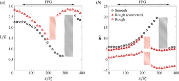
The results are plotted in figure 6. In the upstream regions of zero pressure gradient (ZPG),
 $\widetilde{{\it\kappa}}$
in the smooth case is 0.43, decreasing to 0.36 in the rough case; such a trend and magnitude of the difference agree with the literature. Nagib & Chauhan (Reference Nagib and Chauhan2008) (hereafter referred to as NC08) collected experimental data from various studies of smooth-wall ZPG boundary layers and demonstrated that the slope shows a scatter between around 0.35 and 0.45 for flows with low Reynolds numbers (
 $Re_{{\it\delta}^{\ast }}<4000$
); in addition, Leonardi & Castro (Reference Leonardi and Castro2010) (hereafter referred to as LC10) observed from DNS of channel flows that the slope decreases with the roughness function, from 0.41 to 0.36 for a type of cube roughness. Entering the FPG region, both cases exhibit a similar decrease of the slope for up to
 $x/{\it\delta}_{o}^{\ast }\approx 200$
; this was explained by Nickels (Reference Nickels2004) as the destruction of the constant-stress region, and consequently a decrease of the velocity scale in the logarithmic region. The Reynolds shear stress profiles, which highlight the destruction of the constant-stress region, will be shown later. In addition, the logarithmic region moves away from the wall in wall units (figure 5): in the smooth case at
 $x/{\it\delta}_{o}^{\ast }\approx 50$
, it extends between
 $y^{+}=35$
and
 $y/{\it\delta}=0.2$
, while it moves out of this range at
 $x/{\it\delta}_{o}^{\ast }=220$
. This is due to the thickening of the viscous sublayer, and thus the shortening (and ultimate disappearance) of the overlap region. The rough case resembles the smooth case in the upward shift of the log-law region, as is shown in figure 5(b) for
 $50<x/{\it\delta}_{o}^{\ast }<170$
. This resemblance is due to the residual viscous sublayer, which is not completely destroyed by the roughness in the transitionally rough regime (Jiménez Reference Jiménez2004).
Variation of (a) local logarithmic slope and (b) local intercept. Symbols: ○ smooth case, ▵ rough case. Shaded regions indicate the streamwise regions where the logarithmic profile is not well defined.

After
 $x/{\it\delta}_{o}^{\ast }\approx 200$
, while the smooth-wall slope keeps decreasing throughout the rest of the acceleration region, the rough-wall slope returns to the canonical value (figure 6
a). This early recovery corresponds to the re-establishment of the logarithmic region between
 $y/k=2$
and
 $y/{\it\delta}=0.2$
, as shown in figure 5(b) for
 $x/{\it\delta}_{o}^{\ast }=300$
. This is likely because, as the viscous sublayer disappears, a new overlap region is established between the inner layer (
 $y/{\it\delta}<0.2$
) and the region outside the roughness sublayer (
 $y/k>2$
). In this
 $x$
-region,
 $1/\widetilde{{\it\kappa}}$
tends towards the canonical value due to the recovery of the constant-stress region. Note that during the slope recovery, within a narrow streamwise band, the profile of
 ${\it\Xi}$
shows no local minimum, and the logarithmic region is not well defined; for example, this occurs at
 $x/{\it\delta}_{o}^{\ast }=330$
in the smooth case (figure 5
a) and at
 $x/{\it\delta}_{o}^{\ast }=220$
in the rough case (figure 5
b). This region is shaded in figure 6.
In a canonical boundary layer, the higher drag on the rough wall can be quantified using the roughness function,
 ${\rm\Delta}U^{+}$
, which in ZPG boundary layers, channels and pipes is a function of
 $k_{s}^{+}$
only; it can be used to relate the rough-wall intercept
 $B_{R}$
to the smooth-wall value
 $B_{S}$
:
 $$\begin{eqnarray}{\rm\Delta}U^{+}(x)=B_{S}(x)-B_{R}(x).\end{eqnarray}$$
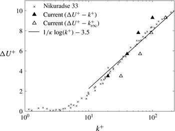
The values of
 ${\rm\Delta}U^{+}$
for
 $k^{+}$
ranging from 20–100 for the present rough surface are collected from channel-flow simulations with this roughness model (Yuan & Piomelli Reference Yuan and Piomelli2014a
,Reference Yuan and Piomelli
c
) and plotted in figure 7. As mentioned earlier,
 ${\rm\Delta}U^{+}$
matches the Nikuradse sandgrain value (
 $k_{s}=k$
) in the transitionally rough regime for
 $k^{+}\leqslant 40$
, and becomes a logarithmic function of
 $k^{+}$
(when the flows enters the fully rough regime) for
 $k^{+}\geqslant 60$
, where the Nikuradse sandgrain with
 $k_{s\infty }=1.6k$
gives the same values of
 ${\rm\Delta}U^{+}$
.
Comparison of the roughness function between the Nikuradse sandgrain and the current numerical sandgrain (Yuan & Piomelli Reference Yuan and Piomelli2014a
,Reference Yuan and Piomelli
c
), whose
 $k_{s\infty }=1.6k$
. The solid line shows the fitted profile for the Nikuradse sandgrain in the fully rough regime (Nikuradse Reference Nikuradse1933).

We use
 ${\rm\Delta}U^{+}$
to correct the intercept in the non-equilibrium boundary layer, by interpolating the
 ${\rm\Delta}U^{+}$
–
 $k^{+}$
relation (figure 7) using the local
 $k^{+}(x)$
shown in figure 3(a). In figure 6(b), the corrected rough-wall intercept,
 $B_{R}(x)+{\rm\Delta}U^{+}(x)$
, is compared with the smooth-wall value. Acceptable agreement is observed in the ZPG regions and, interestingly, in the first part of the acceleration region before the restoration of the canonical value (
 $50<x/{\it\delta}_{o}^{\ast }<220$
). This indicates that the
 ${\rm\Delta}U^{+}$
–
 $k^{+}$
correlation obtained in equilibrium channel flows may also apply to non-equilibrium accelerating flows. This observation also holds in sink flows (Yuan & Piomelli Reference Yuan and Piomelli2014b
) and wall jets (Banyassady & Piomelli Reference Banyassady and Piomelli2014). After the recovery of the rough case and before
 $x/{\it\delta}_{o}^{\ast }=350$
,
 ${\rm\Delta}U^{+}$
fails to correct
 $B_{R}$
to
 $B_{S}$
, since, in this region, the smooth case is in the quasi-laminar region, where
 $B_{S}$
is far from the canonical value.
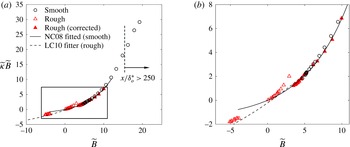
For canonical wall-bounded flows and accelerating or decelerating boundary layers over a smooth wall, Nagib & Chauhan (Reference Nagib and Chauhan2008) showed that
 $\widetilde{{\it\kappa}}\widetilde{B}$
is a function of
 $\widetilde{B}$
, and that effectively only one variable is required to describe the logarithmic profile for a wide range of smooth-wall flows. Figure 8 compares the present data with the NC08 relation. As expected, the smooth-wall data match it well; on the other hand, the uncorrected rough-wall data agree, for
 $\widetilde{B}\leqslant 0.7$
(in the ZPG region), with the modified fit obtained by LC10 from experimental and numerical data of equilibrium channel and boundary layer flows over roughness. For large
 $\widetilde{B}$
(in the FPG region), however, the present data deviate noticeably from the LC10 relation. When the intercept is corrected by
 ${\rm\Delta}U^{+}$
, however, the rough-wall data also match the NC08 relation in both equilibrium and non-equilibrium regions, as shown in figure 8(b). This indicates a possible way to define the roughness function applied for non-equilibrium boundary layers where the logarithmic slope varies: instead of the specific local values of smooth-wall intercept, the roughness function can be obtained by collapsing the
 $\widetilde{{\it\kappa}}\widetilde{B}$
values on the experimental correlation.
(a) Variation of the product of
 $\widetilde{{\it\kappa}}\widetilde{B}$
as a function of the intercept with and without the roughness correction; the arrow denotes the start of the quasi-laminarization. (b) An enlargement focusing on the rough-case data.

3.3. Wake fluctuations
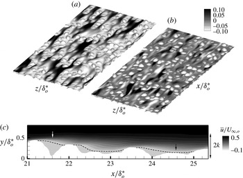
The wake fluctuations result from the small-scale recirculation downstream of the roughness elements. Figure 9 compares the wake fluctuations (figure 9
a) with the turbulent ones (figure 9
b) in the
 $xz$
-plane at
 $y=d$
. In this near-wall region, the turbulence is shown by the low-speed streaks, shortened by the presence of roughness. As expected, the wake fluctuations correlate closely with the roughness geometry. A low-speed region is formed immediately downstream of most of the roughness elements. When the streamwise distance between two tall elements is large enough, the flow reattaches before the next element, as shown by the time-averaged velocity (for example, at
 $x/{\it\delta}_{o}^{\ast }=24.5$
in figure 9
c); this phenomenon leads to the short high-speed streaks (due to the wake component) in figure 9(a). Note that these streaks are different from the turbulent low-speed streaks, which are instantaneous fluctuations from the time-averaged velocity. On the other hand, when two tall elements are close to each other in the streamwise direction (at
 $x/{\it\delta}_{o}^{\ast }=21.5$
in figure 9
c), no reattachment occurs between them. Strong shear layers are present in the vicinity of the roughness crest in the roughness sublayer. These shear layers and recirculation regions were also observed by Chan-Braun, García-Villalba & Uhlmann (Reference Chan-Braun, García-Villalba and Uhlmann2011) in their DNS study. The mean flow channelling phenomenon, similar to the streaks with high-magnitude positive
 $\widetilde{u}$
, was also observed by Hong, Katz & Schultz (Reference Hong, Katz and Schultz2011). In the near-wall region shown in the contours, the peak magnitude of
 $\widetilde{u}$
is of the same order as that of
 $u^{\prime }$
.
Horizontal contours of (a)
 $\widetilde{u}/U_{\infty ,o}$
and (b) instantaneous
 $u^{\prime }/U_{\infty ,o}$
at
 $y=d$
in a streamwise region centred at
 $x/{\it\delta}_{o}^{\ast }=20$
, and (c) contour of the time-averaged velocity,
 $\overline{u}/U_{\infty ,o}$
, in an
 $xy$
-plane, with the dashed line representing the contour line of
 $\overline{u}=0$
. The white and black arrows indicate, respectively, the recirculation between two close elements and the flow reattachment between two elements separated by a greater streamwise distance.

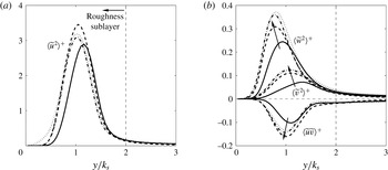
Figure 10 shows
 $y$
-profiles of the dispersive stresses,
 $\langle \widetilde{u}_{i}\widetilde{u}_{j}\rangle$
, normalized by the local
 $u_{{\it\tau}}$
. Four representative streamwise locations are selected: two are in the upstream and downstream ZPG regions (
 $x/{\it\delta}_{o}^{\ast }=0$
and 400), the others in the FPG region (
 $x/{\it\delta}_{o}^{\ast }=200$
and 300). The roughness sublayer is the region in which the dispersive stresses are significant, and its thickness is approximately
 $2k$
. The streamwise-stress profiles,
 $\langle \widetilde{u}^{2}\rangle$
, scaled by the local friction velocity, collapse slightly better than those of the other components (figure 10
a); since the pressure drag is generated by the wake fluctuations in the streamwise direction, the streamwise wake component is expected to be an appropriate velocity scale in the roughness layer. The other two components of the normal dispersive stress increase significantly as the flow accelerates (figure 10
b), possibly due to the decreasing
 ${\it\delta}/k$
that results from the thinning of the boundary layer in the acceleration region (shown in figure 2
a,b). Similar effects of
 ${\it\delta}/k$
on the dispersive stresses were also observed in channel-flow DNS by Yuan & Piomelli (Reference Yuan and Piomelli2014c
). This result is also consistent with the observation by Coceal et al. (Reference Coceal, Thomas, Castro and Belcher2006) in DNS of flows over cube roughness with low submergence (
 ${\it\delta}/h=4$
–6, where
 $h$
is cube height): they found that the dispersive shear stress is approximately
 $0.15u_{{\it\tau}}^{2}$
, more than twice the value observed by Mignot et al. (Reference Mignot, Bartheleemy and Hurther2009) in experiments on channel flows over a gravel bed with high submergence (
 ${\it\delta}/k>40$
).
Profiles of the dispersive stresses, including (a) the streamwise normal component and (b) the other two normal components and the shear component, normalized by local
 $u_{{\it\tau}}$
. ——
 $x/{\it\delta}_{o}^{\ast }=50$
, – – –
 $x/{\it\delta}_{o}^{\ast }=220$
, – - – - –
 $x/{\it\delta}_{o}^{\ast }=300$
,
 $\cdots \cdots$
 $x/{\it\delta}_{o}^{\ast }=400$
. Arrows highlight the direction of the flow acceleration.

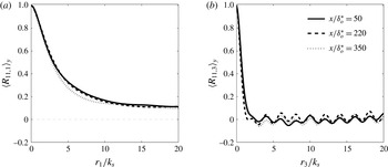
To study the average size of the wake structures, the two-point correlation of
 $\widetilde{u}(x,y,z)$
is calculated, at each
 $(x,y)$
location,
 $$\begin{eqnarray}R_{11}(\boldsymbol{x},\boldsymbol{r})=\frac{\langle \widetilde{u}(\boldsymbol{x})\widetilde{u}(\boldsymbol{x}+\boldsymbol{r})\rangle }{\langle \widetilde{u}^{2}\rangle },\end{eqnarray}$$
where
 $\boldsymbol{r}$
is the separation vector. The correlation is then integrated for
 $0.5\leqslant y/k\leqslant 2$
to obtain its vertically averaged value in the roughness sublayer,
 $\langle R_{11}\rangle _{y}$
. We considered only streamwise and spanwise separations, and the corresponding vertically averaged correlations are
 $\langle R_{11,1}\rangle _{y}$
and
 $\langle R_{11,3}\rangle _{y}$
. The separation is normalized by the roughness height
 $k$
. Figure 11 shows that neither the streamwise nor the spanwise correlation varies in
 $x$
: the integral length scale of the wake fluctuations is affected mainly by the size of the roughness elements, while the pressure-gradient effect is negligible. The correlation length is much larger in
 $x$
than in
 $z$
, due to the effect of the high-speed
 $\widetilde{u}$
streaks discussed above (figure 9
a); in the spanwise direction,
 $\widetilde{u}$
becomes uncorrelated for separations larger than
 $2k$
, reflecting the lateral extent of both low-speed and high-speed regions of
 $\widetilde{u}$
.
Two-point correlations of
 $\widetilde{u}$
with (a) streamwise and (b) spanwise separations, at three
 $x$
locations (
 $x/{\it\delta}_{o}^{\ast }=50$
, 220, 350).

3.4. Turbulence statistics
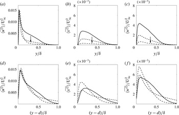
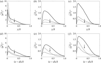
The normal Reynolds stresses in outer scaling are shown in figure 12, at three streamwise locations that cover the FPG region. In the smooth case, the Reynolds stresses decrease significantly in the outer layer relative to
 $U_{\infty }$
, while, on the rough wall, they adjust faster to
 $U_{\infty }$
in this region; the Reynolds-stress profiles change in shape, so no collapse is obtained. Near the wall,
 $\langle \overline{u^{\prime 2}}\rangle$
increases at the same rate as
 $U_{\infty }^{2}$
on both walls; the other two components increase faster than
 $U_{\infty }^{2}$
on the rough wall, while they stay almost unchanged in magnitude (and thus decrease under this scaling) on the smooth wall. These trends are consistent with the more homogeneous redistribution of TKE into its components in rough-wall turbulence, observed by several researchers (Shafi & Antonia Reference Shafi and Antonia1995; Schultz & Flack Reference Schultz and Flack2007). The fact that all components in the other layer are higher on the rough wall than on the smooth wall is also consistent with the results of Cal et al. (Reference Cal, Brzek, Johansson and Castillo2009); they also observed that, different from the present results, the acceleration effect is absorbed by the normalization using
 $U_{\infty }$
, due to the much weaker acceleration and the quasi-equilibrium state of their boundary layers.
Profiles of normal Reynolds stresses, normalized by local
 $U_{\infty }$
: (a–c) smooth; (d–f) rough. ——
 $x/{\it\delta}_{o}^{\ast }=50$
; – – –
 $x/{\it\delta}_{o}^{\ast }=200$
; – - – - –
 $x/{\it\delta}_{o}^{\ast }=300$
. The arrow indicates the direction of flow acceleration.

Figure 13 compares the normal Reynolds stresses, normalized by the local friction velocity. Similar to what was observed by Cal et al. (Reference Cal, Brzek, Johansson and Castillo2009), the normalized Reynolds stress in the outer layer decreases in the FPG region in both cases, showing that turbulence increases more slowly than the drag. In the rough case, this also means that the turbulence lags behind the development of the wake field.
Profiles of normal Reynolds stresses, normalized by local
 $u_{{\it\tau}}$
: (a–c) smooth; (d–f) rough. ——
 $x/{\it\delta}_{o}^{\ast }=50$
; – – –
 $x/{\it\delta}_{o}^{\ast }=200$
; – - – - –
 $x/{\it\delta}_{o}^{\ast }=300$
. The arrow indicates the direction of flow acceleration.

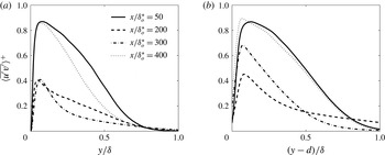
The Reynolds shear stress, normalized by the local friction velocity, is shown in figure 14. On the smooth wall, it decreases significantly throughout the acceleration region, while in the rough case, after an initial decrease, it starts to recover at
 $x/{\it\delta}_{o}^{\ast }\approx 220$
; the recovery appears to originate from the near-wall region and spread outward. In both cases, a change of shape towards the sink-flow profile (Spalart Reference Spalart1986; Yuan & Piomelli Reference Yuan and Piomelli2014b
) is observed, characterized by the sharper peak and the disappearance of a constant-stress region, as mentioned earlier. This shape change of the Reynolds shear stress can be explained by the impact of the pressure gradient on the near-wall total shear stress (Nickels Reference Nickels2004). At
 $x/{\it\delta}_{o}^{\ast }=400$
, the ZPG state is almost recovered in both cases.
Profiles of Reynolds shear stress in (a) smooth and (b) rough cases, normalized by
 $u_{{\it\tau}}$
. ——
 $x/{\it\delta}_{o}^{\ast }=50$
; – – –
 $x/{\it\delta}_{o}^{\ast }=200$
; – - – - –
 $x/{\it\delta}_{o}^{\ast }=300$
;
 $\cdots \cdots$
 $x/{\it\delta}_{o}^{\ast }=400$
.

3.5. Reynolds-stress anisotropy
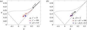
The streamwise evolution of the Reynolds-stress anisotropy tensor
 $$\begin{eqnarray}\unicode[STIX]{x1D623}_{ij}=\frac{\langle \overline{u_{i}^{\prime }u_{j}^{\prime }}\rangle }{\langle \overline{u_{k}^{\prime }u_{k}^{\prime }}\rangle }-\frac{1}{3}{\it\delta}_{ij},\end{eqnarray}$$
during acceleration is shown in figure 15, in terms of its second and third invariants (Lumley Reference Lumley1978),
 $$\begin{eqnarray}{\it\eta}^{2}=-{\textstyle \frac{1}{6}}\unicode[STIX]{x1D623}_{ij}\unicode[STIX]{x1D623}_{ji},\quad {\it\xi}^{3}={\textstyle \frac{1}{6}}\unicode[STIX]{x1D623}_{ij}\unicode[STIX]{x1D623}_{jk}\unicode[STIX]{x1D623}_{ki}.\end{eqnarray}$$
Three wall-normal locations are considered: one in the outer region (
 $y/{\it\delta}=0.5$
), one in the logarithmic region,
 $(y-d)^{+}=100$
, and the last very near the wall,
 $(y-d)^{+}=15$
for the smooth case and
 $y/k=2$
for the rough one. On the smooth wall, turbulence develops towards one-dimensional (1D) turbulence in the logarithmic region and below, almost reaching the 1D state (the upper right corner of the triangle) near the wall. In contrast, on the rough wall the anisotropy in the logarithmic region is unaffected, while near the roughness crest it shifts towards the isotropic state (the lowest vertex of the triangle). It should be pointed out that, although the turbulence becomes more isotropic, the streaky structures of the time-averaged velocity are maintained throughout the acceleration process (figure 11) since they are due to the wall geometry.
The evolution of Reynolds-stress invariants at three wall-normal locations for
 $50\leqslant x\leqslant 330$
: (a) smooth and (b) rough cases. Symbols show the most upstream location. Arrows indicate the direction of increasing
 $x$
.

To explain the difference in Reynolds-stress anisotropy, we investigate the Reynolds-stress budget. The budget of Reynolds stresses and TKE were derived by Raupach & Shaw (Reference Raupach and Shaw1982) for flow over a canopy and by Mignot et al. (Reference Mignot, Bartheleemy and Hurther2009) for flow over roughness. The budgets of the normal Reynolds stresses,
 $\langle \overline{u_{{\it\alpha}}^{\prime 2}}\rangle$
, in a boundary layer are
 $$\begin{eqnarray}\displaystyle & & \displaystyle -\frac{\partial }{\partial x_{j}}\langle \overline{u}_{j}\rangle _{s}\langle \overline{u_{{\it\alpha}}^{\prime }u_{{\it\alpha}}^{\prime }}\rangle -\frac{\partial }{\partial x_{j}}\langle \overline{u_{{\it\alpha}}^{\prime }u_{{\it\alpha}}^{\prime }u_{j}^{\prime }}\rangle _{s}-\frac{\partial \langle \widetilde{u_{{\it\alpha}}^{\prime }u_{{\it\alpha}}^{\prime }}\widetilde{u}_{j}\rangle _{s}}{\partial x_{j}}-2\langle \overline{u_{{\it\alpha}}^{\prime }u_{j}^{\prime }}\rangle \frac{\partial \langle \overline{u}_{{\it\alpha}}\rangle _{s}}{\partial x_{j}}\nonumber\\ \displaystyle & & \displaystyle \quad -\,2\left\langle \widetilde{u_{{\it\alpha}}^{\prime }u_{j}^{\prime }}\frac{\partial \widetilde{u}_{{\it\alpha}}}{\partial x_{j}}\right\rangle _{s}-2\left\langle \overline{u_{{\it\alpha}}^{\prime }\frac{\partial P^{\prime }}{\partial x_{{\it\alpha}}}}\right\rangle _{s}+{\rm\nabla}^{2}\langle \overline{u_{{\it\alpha}}^{\prime }u_{{\it\alpha}}^{\prime }}\rangle _{s}-{\it\epsilon}_{{\it\alpha}{\it\alpha}}=0\end{eqnarray}$$
(no summation on Greek indices). Here,
 ${\it\epsilon}_{{\it\alpha}{\it\alpha}}$
is the viscous dissipation rate of
 $\langle \overline{u_{{\it\alpha}}^{\prime 2}}\rangle$
. The wake production,
 $P_{w}=2\langle \widetilde{u_{{\it\alpha}}^{\prime }u_{j}^{\prime }}(\partial \widetilde{u}_{{\it\alpha}}/\partial x_{j})\rangle _{s}$
, appears with a positive sign in the budgets of the normal dispersive stresses and represents the energy exchange between the turbulent and wake fields.
The wake fluctuations interact with turbulent fluctuations in two ways (Finnigan Reference Finnigan2000): first, the turbulent structures with scales larger than the wake scale work against the form drag, converting TKE to wake kinetic energy (WKE); at the same time, the WKE is converted through energy cascade to TKE associated with structures with scales smaller than the wake structures. The wake production represents the net conversion between TKE and WKE. Yuan & Piomelli (Reference Yuan and Piomelli2014c
) observed, in DNS of a transitionally rough open-channel flow, that
 $P_{w}$
is negative for the streamwise normal Reynolds stress, probably because this Reynolds-stress component is mostly associated with larger-scale turbulent structures, converting TKE to WKE; on the other hand,
 $P_{w}$
is positive for the wall-normal and spanwise components of Reynolds stress, since these two components are associated with smaller-scale turbulent structures, and more WKE is converted to TKE through energy cascade.
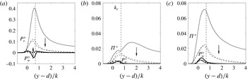
The effects of acceleration on the source terms of the three Reynolds-stress components are shown in figure 16. In the upstream ZPG region (
 $x/{\it\delta}_{o}^{\ast }=50$
), the Reynolds-stress budgets are consistent with the picture above. As the flow accelerates, the shear production decreases, mostly due to the decrease of Reynolds shear stress compared to
 ${\it\tau}_{w}$
(figure 14
b), i.e. turbulence adjusts to the acceleration more slowly than the drag. For the same reason, the pressure work,
 ${\it\Pi}_{{\it\alpha}{\it\alpha}}=-2\langle \overline{u_{{\it\alpha}}^{\prime }(\partial P^{\prime }/\partial x_{{\it\alpha}})}\rangle _{s}$
, decreases outside of the roughness sublayer. However,
 ${\it\Pi}_{22}$
adapts faster to the inner scaling below the roughness crest,
 $k_{c}$
; this is presumably due to both the intensification of
 $v^{\prime }$
, as a result of turbulence–wake interactions, and an increase of
 $P^{\prime }$
intensity, resulting from the addition of the wake-related terms (the second and fourth terms) in the source of the
 $P^{\prime }$
Poisson equation,
 $$\begin{eqnarray}{\rm\nabla}^{2}P^{\prime }=-2\frac{\partial \langle \overline{u}_{i}\rangle }{\partial x_{j}}\frac{\partial u_{j}^{\prime }}{\partial x_{i}}-2\frac{\partial \widetilde{u}_{i}}{\partial x_{j}}\frac{\partial u_{j}^{\prime }}{\partial x_{i}}-\frac{\partial ^{2}}{\partial x_{i}\partial x_{j}}(u_{i}^{\prime }u_{j}^{\prime }-\langle \overline{u_{i}^{\prime }u_{j}^{\prime }}\rangle )-\frac{\partial ^{2}\widetilde{u_{i}^{\prime }u_{j}^{\prime }}}{\partial x_{i}\partial x_{j}}.\end{eqnarray}$$
It is also worth noting that both the shear production and the pressure work peak around the roughness crest. The wake production becomes less important for
 $\langle \overline{u^{\prime 2}}\rangle$
, but more so for
 $\langle \overline{v^{\prime 2}}\rangle$
and
 $\langle \overline{w^{\prime 2}}\rangle$
, probably because the further separation between the roughness length scale and the viscous length scale (as
 $k^{+}$
increases) leads to a larger amount of WKE being converted to TKE through energy cascade from
 $k$
towards the Kolmogorov scale.
Effects of FPG on budget terms of (a)
 $\langle \overline{u^{\prime 2}}\rangle$
, (b)
 $\langle \overline{v^{\prime 2}}\rangle$
and (c)
 $\langle \overline{w^{\prime 2}}\rangle$
, normalized in wall units. ——
 $x/{\it\delta}_{o}^{\ast }=50$
, – – –
 $x/{\it\delta}_{o}^{\ast }=200$
, – - – - –
 $x/{\it\delta}_{o}^{\ast }=300$
. Arrows show the direction of flow acceleration.

To explain the fact that the FPG does not increase the flow anisotropy in the roughness sublayer, we should consider the effects of both the persistent wake production (which does not vanish as the flow accelerates) and the near-wall pressure work, which remains significant, unlike the smooth case, in which it diminishes under strong FPG (Piomelli & Yuan Reference Piomelli and Yuan2013). Both these effects contribute to more even redistribution of TKE among the three directions. The pressure work appears to be the leading factor here, due to its higher magnitude. However, the contribution of wake production may increase for flows with higher Reynolds number, as indicated by figure 16(b,c) and also by the observation that, for a higher
 $k^{+}$
,
 ${\it\Pi}^{+}$
decreases whereas
 $P_{w}^{+}$
is almost unchanged (Yuan & Piomelli Reference Yuan and Piomelli2014c
).
Ratio between the time scales of the turbulence, the wake shear, and the mean shear in (a) the smooth case and (b) the rough case. ——
 $x/{\it\delta}_{o}^{\ast }=50$
, – – –
 $x/{\it\delta}_{o}^{\ast }=220$
, – - – - –
 $x/{\it\delta}_{o}^{\ast }=300$
. Thick lines:
 $S^{\ast }$
; thin lines:
 $S_{w}^{\ast }$
. Arrows indicate increasing
 $x$
.

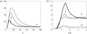
The difference in turbulence anisotropy can also be explained by the different importance of the mean shear compared to the shear of the turbulence (namely, by the ratio between the time scale of the turbulence and that of the mean shear),
 $$\begin{eqnarray}S^{\ast }=\frac{\overline{S}q^{2}}{2{\it\epsilon}},\end{eqnarray}$$
where
 $\overline{S}=2(\overline{\unicode[STIX]{x1D61A}}_{ij}\overline{\unicode[STIX]{x1D61A}}_{ij})^{1/2}$
is the mean strain rate,
 $\overline{\unicode[STIX]{x1D61A}}_{ij}=(\partial \langle \overline{u}_{i}\rangle /\partial x_{j}+\partial \langle \overline{u}_{j}\rangle /\partial x_{i})/2$
is the strain-rate tensor,
 $q=\langle \overline{u_{i}^{\prime }u_{i}^{\prime }}\rangle ^{1/2}$
and
 ${\it\epsilon}$
is the dissipation rate of TKE. For homogeneous turbulence under a strong uniform mean shear, the eddies are distorted by the flow sufficiently rapidly that the turbulence is not significantly modified by the change in strain rate through the production terms, but it is modified by the stretching of the individual vortex elements; a development towards 1D turbulence (with all TKE in
 $u^{\prime }$
) then follows (Hunt Reference Hunt1978). Lee, Kim & Moin (Reference Lee, Kim and Moin1990) compared a boundary layer with a homogeneous turbulent flow with uniform shear, and concluded that these effects of strong mean shear also apply to a near-wall region in a turbulent shear flow. Figure 17 compares
 $S^{\ast }$
in the present cases. In the smooth case,
 $S^{\ast }$
peaks at the top of the viscous sublayer and asymptotes to a constant value of around 4.5 in the logarithmic region; this constant results from the fact that
 $-\langle \overline{u^{\prime }v^{\prime }}\rangle /q^{2}\approx 0.15$
, the TKE production
 $\mathscr{P}\approx -\langle \overline{u^{\prime }v^{\prime }}\rangle \partial U/\partial y$
and
 $\mathscr{P}\approx {\it\epsilon}$
. This peak value reaches 60 in the quasi-laminarization region, significantly affecting the turbulent eddy shape and the Reynolds-stress anisotropy. In the rough case, the peak of
 $S^{\ast }$
is located at the roughness crest (
 $1.5k$
), and decreases with acceleration towards the value in the logarithmic region (4.5), as the logarithmic region reaches the top of the roughness sublayer when the fully rough regime is achieved. The ratio between the time scale of turbulence and that of the wake strain rate,
 $$\begin{eqnarray}S_{w}^{\ast }=S_{w}q^{2}/2{\it\epsilon}\end{eqnarray}$$
(where the shear of the wake
 $S_{w}(x,y)$
is approximated as
 $\langle \widetilde{u}^{2}\rangle ^{1/2}/k$
), is also plotted in figure 17(b).
 $S_{w}^{\ast }$
peaks inside the roughness sublayer, with values of the order of one. Note that the non-zero
 $S_{w}^{\ast }$
outside the roughness sublayer is due to the finite temporal sampling. These observations indicate that neither the mean shear nor the wake strain is sufficient to result in a significant change of Reynolds-stress anisotropy in the rough case.
4. Conclusions and discussions
A direct numerical simulation is carried out on a flat-plate turbulent boundary layer over roughness with strong non-equilibrium free-stream acceleration, to investigate the effects of the strong FPG on a rough-wall boundary layer. Such acceleration leads to quasi-laminarization on a smooth wall. But roughness prevents the flow reversion. Instead, the acceleration leads to higher
 $C_{f}$
, faster increase of TKE compared to
 $U_{\infty }^{2}$
and more isotropic turbulence near the roughness crest.
It is shown that the roughness leads to a wake field that is persistent throughout acceleration. The intensity of the wake scales mostly with the friction velocity, and the integral length scale scales with the roughness length scale. The wake promotes the Reynolds-stress isotropy in two ways. First, it increases
 $v^{\prime }$
and
 $w^{\prime }$
through a production mechanism transferring wake energy to turbulence. In addition, it gives rise to an augmentation of the pressure work term and more even redistribution of TKE in the three directions. As a result, the wake field maintains the inner–outer-layer interactions and the turbulence production cycle through instability mechanisms (Jiménez & Pinelli Reference Jiménez and Pinelli1999; Bourassa & Thomas Reference Bourassa and Thomas2009).
The mean-velocity profile departs from the universal logarithmic profile for both cases during acceleration. In the transitionally rough regime, it varies in a way similar to the smooth case, including a decrease of
 $1/\widetilde{{\it\kappa}}$
and upward shift of the logarithmic region, due to the residual viscous sublayer. After the fully rough regime is reached,
 $\widetilde{{\it\kappa}}$
returns to the canonical value, associated with a newly established overlap region between the inner layer,
 $y/{\it\delta}<0.2$
, and the outer layer,
 $y/k>2$
. The
 ${\rm\Delta}U^{+}$
–
 $k^{+}$
correlation, obtained from the equilibrium state, can be applied to the present non-equilibrium boundary layer to restore the smooth-wall relationship between
 $\widetilde{{\it\kappa}}$
and
 $\widetilde{B}$
. This may have indications in determining the rough-wall drag in turbulence models.
The effects of the acceleration and roughness are closely coupled. The acceleration leads to an increase of the mean strain rate (most importantly, the mean shear rate,
 $\partial U/\partial y$
), and tends to stabilize the near-wall turbulence by linearly stretching the turbulent eddies, which results in relaminarization on a smooth wall (Hunt Reference Hunt1978; Lee et al.
Reference Lee, Kim and Moin1990; Piomelli & Yuan Reference Piomelli and Yuan2013). As an opposite effect, acceleration in the free stream causes the increase of mean velocity at the top of the roughness sublayer,
 $U_{RS}$
, which is shown to linearly promote the wake intensity in the fully rough regime. On the other hand, roughness reduces the time scale of the turbulence near the wall, resulting in turbulence that is more responsive to the mean flow variations; this counteracts the FPG effect in linear stretching of the turbulent structures. As a result, the combined effects are a higher
 $\partial U/\partial y$
, which impacts the turbulence mainly through a higher production, and an increase of wake intensity, which leads to higher pressure drag and higher transfer between the energy of the wake and that of the turbulence.
The coupling described above, however, does not apply if the roughness effect is weak on the boundary layer before coming into the acceleration region: for a boundary layer with a similar acceleration distribution but a weaker roughness effect at the inlet (indicated by a lower
 $k_{s,o}^{+}$
value of 7 compared to the present value of 23), Piomelli & Yuan (Reference Piomelli and Yuan2013) observed that FPG leads to an initial increase of
 $C_{f}$
, followed by a decrease until it reaches the smooth-wall value. This is because, in the lower limit of the transitionally rough regime, a large number of quasi-streamwise vortices survive the disturbance due to the roughness, without breaking up into smaller eddies; they are stretched by the increased mean shear, similar to the vortices near a smooth wall; had the FPG region been sufficiently long, complete relaminarization would probably have been achieved. On the other hand, if the upstream boundary layer is near or inside the fully rough regime, a spectrum of turbulent eddies are generated as the wake field constantly bends the near-wall vortices and causes them to collide, regardless of acceleration, which has been shown here not to be able to eliminate the wake shear; in this case, the flow reversion is not expected, even with a stronger FPG or a longer FPG region.
The variation in the combined effects in different flow states (i.e. equilibrium or not) may now be explained by the difference in the acceleration history, which affects the variation of
 $U_{RS}$
. In the present non-equilibrium boundary layer,
 $U_{RS}$
increases faster than the free stream due to the flow entrainment and a thinner boundary layer; this results in a ‘rougher’ flow, as well as higher
 $C_{f}$
, higher turbulence intensity, and lower Reynolds-stress anisotropy. Similar observations in a spatially developing flow by Cal et al. (Reference Cal, Brzek, Johansson and Castillo2009) support this theory. Tachie & Shah (Reference Tachie and Shah2008) also reported the increase of drag. In a sink flow, on the other hand,
 $U_{RS}$
decreases (relative to
 ${\it\nu}/k$
) with
 $K$
due to the decrease of flow rate
 $Q$
, as
 $K={\it\nu}/Q$
; thus
 $k^{+}$
decreases, and the flow tends towards the hydraulically smooth regime and laminarization (Yuan & Piomelli Reference Yuan and Piomelli2014b
).
This study considers a scenario more realistic than canonical rough-wall boundary layers. Although different flow behaviours result from the added complexity under different free-stream conditions, they point to the same underlying physics, which may also help explain the flows in other realistic rough-wall boundary layers, such as those with adverse pressure gradient and rotation.
Acknowledgements
Support from Hydro Québec, the Natural Science and Engineering Research Council of Canada (NSERC) and the High Performance Computing Virtual Laboratory (HPCVL) is acknowledged. U.P. gratefully acknowledges the support of the Canada Research Chairs program.