

From the seminal study of Martha's Vineyard (Labov, Reference Labov1963, Reference Labov1972) onward, it has been a common assumption that different variables can show different behavior in terms of the rate of change. Although sociolinguistic studies have often considered the dynamics of several variables in various speech communities (Dorian, Reference Dorian1994; Kerswill & Williams, Reference Kerswill and Williams2005; Lippi-Green, Reference Lippi-Green1989; Milroy, Reference Milroy1987; Nahkola & Saanilahti, Reference Nahkola and Saanilahti2004; Sundgren, Reference Sundgren2009; Trudgill, Reference Trudgill1974), the comparison has usually been made impressionistically rather than on a statistically informed basis.
The comparison of trajectories of change of different variables is an important step in gaining a deeper understanding of language change. First, it goes toward a comparison of scenarios of language change in different languages and varieties. Second, a comparison of variable trajectories is the logical prerequisite for studying the role and interaction of factors that underlie changes on a more abstract level and affect more than one variable.
The so-called “fixed route hypothesis” stipulates that there is a certain hierarchy by which variables are lost across speakers (Trudgill, Reference Trudgill1986:20), as captured in implicational scales (Rickford, Reference Rickford, Chambers, Trudgill and Schilling2002); however, the implicational models involved are suitable only for categorical data, not for corpus frequencies as used here. Other studies that used statistically elaborate methods to compare variables are Labov, Rosenfelder, and Fruehwald (Reference Labov, Rosenfelder and Fruehwald2013), who, however, primarily focused on how dynamics of individual variables depend on sex or education level; and Fruehwald (Reference Fruehwald2017), who compared different variables with a view to detect their sensitivity to lifespan and generational change rather than to compare their general characteristics.
In our paper, we propose three characteristics to facilitate the comparison of variables: (a) initial level, that is, the proportion between dialect and standard realizations at the beginning of the observation; (b) steepness, that is, how fast or slow the change takes place, and (c), turning point, that is, the years of birth after which the standard realization of a variable starts to dominate. All these measures have confidence intervals and are derived from the logistic regression model in a straightforward way. They constitute language independent tools to compare across variables in a situation of language change.
We present an apparent-time study of variation in a northern Russian rural community tracing 11 phonological and morphological variables in the speech of 33 speakers of different ages, genders, and educational backgrounds, in a total of 16,440 annotated tokens. The variables are exponents of a shift from the preconvergence variety (referred to as the ‘base dialect’ below) to standard Russian which has taken place in this village, as in most of European Russia, in the course of the twentieth century. As the speech community is rather small (official statistics give a population of 488 people for the whole municipality), the study provides a comprehensive picture of language change in progress. We show that all variables undergo a decrease on dialectal realizations, with different rates for different variables.
The community and the dialect
The data for this study comes from a conglomerate of four villages on opposite banks of the river Ustja in the south of Arkhangelsk oblastFootnote 2 of European Russia, around 70 km north of the nearest railroad station at Kostylevo, around 1,000 km northeast of Moscow and around 500 km south of Arkhangelsk, Mikhalevskaya (Iljina) and Isajevskaya (Pushkino) on the one side of Ustja, Karpovskaya (Korostino) and Pir'atinskaya (Kor'akino) on the other. Below, we will use the name Mikhalevskaya to refer to all four villages, as most maps do. In the recent past, the villages formed one collective farm and shared primary school (grades 1–4, from 6 to 9 years old), kindergarten, medical office, and a community center (dom kul'tury). For this paper, we also include data from the village Plosskoe, about four kilometers down the river from Mikhalevskaya. The villages are tightly connected, share a secondary school (grades 5–9; since the 1950s) and belong to the same rural administrative unit. Mikhalevskaya and Plosskoe do not have apparent dialectal distinctions.
Intensive exposure to urban culture started in the second half of the nineteenth century. At that time, the influence of the standard language on regional varieties was noticed in male speakers, whose mobility was higher than that of women (cf., Bubrikh, Reference Bubrikh1914:25–26; Grinkova, Reference Grinkova and Obnorskij1947:371). From the 1930s, the influence of the standard was channeled through the growing presence of education and mass media and occupations other than traditional husbandry.
On the other hand, starting from 1932, outgoing mobility became more restricted. Villagers did not have passports entitling them to travel until the 1970s; to leave the village, they had to obtain a written permission from the collective farm office. They were again allowed to leave the village for temporary employment after the 1950s, when the village youth started to be recruited into construction work, peat processing, etc. The closest railway line Konosha-Kotlas, seventy kilometers to the south, was finished in the early 1940s, but the villages were connected to the railway station by road only in the 1970s. This has all contributed to the preservation of the dialect.
Among our consultants born before World War 2, the vast majority had at most four years of schooling, and often less. All had been doing agricultural work at the collective farm. A very small number of people in this generation, after finishing seven years of school and vocational training outside of the village, ended up with nonhusbandry occupations. Most villagers born after 1950 have had nine years of schooling; some of them also went to three-year occupational courses. Most men were professional drivers and tractor operators; this required two to six months of additional training. Men did two-year military service. Women's nontraditional occupations were more diverse and required longer training outside of the village.
The early 1930s brought the collectivization of private farms. As a result of Stalinist repressions, war, and the famine in 1946–47, the countryside was decimated and impoverished. These demographic changes are reflected in our data. Among our consultants, more people were born in the 1920s than in the 1930s, and no one was born in the years of war. After the collapse of the USSR, the village was hit by unemployment and increased outmigration. In Mikhalevskaya, the kolkhoz has collapsed, and the school has shut down. The overall population of the four villages is now under 200 people, a decrease by half only in the last ten years.
The Ustja dialect belongs to the Vologda group of Northern Russian dialects; see Gecova (Reference Gecova1997) and Sologub (Reference Sologub and Orlova1970:255–261) for surveys of its phonetic and grammatical features. The Atlas of Russian Dialects (DARJA) covers the villages of Bestuzhevo and Saburovo, four and thirty kilometers respectively from Mikhalevskaya. Its maps and supplementary data show that the speech of the 19 women interviewed in 1958, born between 1869 and 1915, already exhibited variation between dialect and standard for some variables.
The corpus and the sample of speakers
This study is based on recordings of mostly biographic interviews collected during four joint Swiss-Russian field tripsFootnote 3 in 2013–2016. They were transcribed in standard Russian orthography and analyzed for particular variables by students of the School of Linguistics (HSE University),Footnote 4 and made available in the searchable Ustja River Basin corpus together with the audio data (www.parasolcorpus.org/Pushkino; von Waldenfels, Daniel, & Dobrushina [Reference von Waldenfels, Daniel and Dobrushina2014], henceforth URB). As of March 2017, 97 hours of interviews have been transcribed, comprising close to 800,000 words from 62 speakers.
For this study, we selected 33 speakers whose speech was sufficiently well represented in the corpus and who lived most of their lives in Mikhalevskaya and Plosskoe. This included a number of elderly women who were born in other villages not far away (Fomin Pochinok, Kadyevskaya) and married into Mikhalevskaya at an early age; we see no evidence that potential differences between the dialects may be relevant in respect to the analysis.
The amount of data available differs depending on speaker and variable, ranging from 80 to 1295 observations, with a median of 500. Variables are represented by data sets ranging from 722 to 2963 annotated tokens, with a total of 16,440 data points. The names of the speakers are coded by an abbreviation which contains their year of birth.
Variables
We consider 11 variables that each are defined to have dialectal and standard realizations in the speech community. We chose such variables that were (a) well represented in the data, and (b) relatively easily classified as either dialectal or standard realizations. We list variables here with the abbreviation by which they are referenced later:
• REFL1: vowel quality in the reflexive morpheme. In the dialect, the reflexive affix contains /e/ as opposed to /a/ in the standard language (dial. ꞌmɯ-w-sʲe versus standard ꞌmɨ-lˠ-sʲə, ꞌmɨ-lˠ-sə ‘wash (Pst, M, Refl)’), 2463 tokens.
• REFL2: retention of vowel in reflexive morpheme. In the dialect, the unreduced form -sʲV (-/sʲе/ or -/sʲа/) is used in all positions. In the standard, the reflexive morpheme -/sʲa/ is reduced to -/sʲ/ if the base ends in a vowel unless it is a participle (dial. ꞌmɯ-l-a-sʲe or ꞌmɯ-l-a-sʲa versus standard ꞌmɨ-lˠ-a-sʲ ‘wash (Pst, F, Refl)’), 1767 tokens.
A salient dialect feature of Arkhangelsk and Vologda dialects is a discourse enclitic particle that is realized as -ot, -ta, -to, -tu, -tʲe depending on the grammatical and phonological properties of its host. In standard Russian, the equivalent particle -/to/ is invariantly used with any host. We consider two variables based on dialectal realizations of the enclitic particle that are both frequent and phonetically unambiguous:
• OT: postposed particle as -/ot/. In the dialect, the enclitic particle is realized as -/ot/ when hosted by singular masculine nouns, adjectives, and pronouns in the nominative/accusative case that end in a consonant; in the standard, it is invariably realized as -/to/, phonetically -[tə] (dial. ꞌdom-ot versus standard ꞌdom-tə ‘house (Nom, Sg, Ptcl)’), 1147 tokens.
• TU: postposed particle as -/tu/. In the dialect, the enclitic particle is realized as -/tu/ when hosted by singular feminine nouns in the accusative as well as by any wordform ending in [u]; in the standard, it is invariably realized as -/to/, phonetically -[tə] (dial. ʐeꞌnu-tu ‘wife (Acc, Sg, Ptcl)’, ꞌmatʲerʲ-tu ‘mother (Acc, Sg, Ptcl)’, ꞌfsʲudu-tu ‘everywhere (Ptcl)’ versus standard ʐɨꞌnu-tə ‘wife (Acc, Sg, Ptcl)’), 722 tokens.
• ADJ: contraction of adjective endings. Somewhat simplifying matters, the ending of nominative singular feminine adjectives -/aja/ is contracted ([a]) or hiatic ([aa]) in the dialect. In the standard, the ending -/aja/ is realized as [ꞌaῐə] or hiatic [ꞌaæ], [əε], with no contraction (dial. moloꞌd aa, moloꞌda versus standard məlˠaꞌdaĭə, məlˠaꞌdaæ ‘young (Fem, Sg, Nom)’), 2974 tokens.
• PREP: absence of epenthetic /nʲ/ after prepositions. In the dialect, third person pronouns have initial /j/- after a preposition, in the standard they have initial /nʲ/- (dial. u jeꞌvo versus standard u nʲiꞌvo ‘by him (Gen)’), 1015 tokens.
• NOM: pronominal nominative plural ending. In the dialect, the nominative plural of the 3rd person pronoun and of the numeral/pronoun odin ‘one, only’ has the ending -/e/ while its standard ending is -/i/ (dial. oꞌnʲe ‘they’, odꞌnʲe ‘some’ versus standard aꞌnʲi, adʲꞌnʲi), 968 tokens.
• A~E: raising of /a/. In the dialect, stressed /a/ (etymological *ę and *a) has been raised to /e/ between palatalized consonants; in the standard, /a/ is retained in this position (dial. ꞌpʲetʲero versus standard ꞌpʲatʲərə ‘five (collective)’), 2555 tokens.
• E~I: raising of yat (*ě). In the dialect, stressed etymological *ě (known as yat; assumed pronunciation close mid [е] or diphthong [ie]) has been raised to /i/ between palatalized consonants, while in the standard it has merged with /e/ (dial. ꞌsʲij е lʲi versus standard ꞌsʲeilʲi ‘sow (Pst, Pl)’), 1194 tokens.
• SH (retroflex sibilant). In the dialect, the long unvoiced sibilant is realized as nonpalatalized retroflex [ʂt͡ʂ] or [ʂː] while in the standard, the sibilant in question is realized as an palatо-alveolar [ʃʲː] (dial. ꞌʐenʂt͡ʂɨna or ꞌʐenʂːɨna vs. standard ꞌʐenʲʃʲːinə ‘woman’), 2963 tokens.
• DISS: dissimilation of /kt/. In the dialect, the unvoiced stop /k/ is realized as [x] before [t] in the pronoun kto ‘who’; in the standard, [k] is retained (dial. xto versus standard kto ‘who’), 998 tokens.
In terms of corpus frequency, these 11 variables vary from quite frequent (REFL1, reflexive vowel quality) to very infrequent (E/I, yat-raising). For all variables except (REFL1) and (REFL2, reflexive vowel retention), all data from each speaker were used in the analysis.
Different corpus queries in CQP were used to extract the relevant wordforms. For instance, for the PREP variable (absence of /nʲ/ after prepositions), all examples where a third person pronoun follows a preposition were extracted. For E/I (yat-raising), the query was based on a list of lexical items that contain etymological *ě.
All occurrences were transcribed based on perception and, in some cases, instrumental analysis in Praat. For most variables, the transcriptions were cross-validated by at least one more member of the project and differences in judgment were subsequently resolved by joint decision. Variation was reduced to binary choice and each example classified as either dialectal or standard.
Note that even the speakers in the oldest generation are not categorical users of the dialectal variants. Among these speakers (year of birth 1920–1930), some variables are almost consistently realized as dialectal (e.g., nonpalatalized retroflex sibilant with SH), while others have high rates of standard realizations (e.g., E/A [a-raising], E/I [yat-raising], REFL2 [reflexive vowel retention], and ADJ [adjective contraction]). Variation in the realization of these latter variables is attested already in the DARJA data from the 1950s (see above) for the Ustja region. This might be either because of convergence to the standard in an earlier stage or because of variation present in the base dialect prior to contact with the standard. For example, there is reason to believe that the use of the unreduced reflexive morpheme (our REFL2 variable) was never across-the-board. However, the conditions of any dialect-internally conditioned variation are presently unknown. In our study, we assume as a hypothetical starting point the exceptionless use of what we defined as the dialectal realizations of each variable (but see discussion in the section that introduces the notion of initial level below).
ANALYSIS
In this section, we show that (a) in all variables, there is a correlation between the age of the speaker and the degree of dialect preservation, and (b) some dialectal features are lost more quickly (in various senses) than others. We suggest three measures that characterize the rate of loss of each variable and allow us to compare them: initial level, steepness, and turning point.
Specifically, we apply the binomial logistic regression model, with age as a fixed effect and speaker as a random effect. The model shows not only the expected correlation of dialect loss with decreasing age but also provides less trivial results on statistically significant differences in the dynamics of dialect loss in individual variables. For each variable, the model shows how abrupt the change was, what the state of dialect preservation in our oldest speakers is, and which generation of speakers ceased to be predominantly dialectal.
We first motivate our approach by exposing the difficulties with direct comparisons of proportion of dialectal realizations of different speakers. We then introduce the logistic regression model, a standard way to show correlation of a noncontrolled set of observations of a binary variable with a scalar factor including time. Finally, we explore the possibilities of comparing the results of the logistic regression analysis across variables.
Why token counts are not enough
Let us start with an intuitively plausible model, namely, we simply compare the relative share of dialectal realizations for each speaker as proportions. Figure 1 plots year of birth against the ratio of dialectal realizations of the PREP variable (absence of /nʲ/ after preposition).
PREP variable (absence of epenthetic /nʲ/ after prepositions): percentages of dialectal realizations by speakers’ year of birth. Unshaded speakers are those discussed below in this section; all other speakers are shaded.

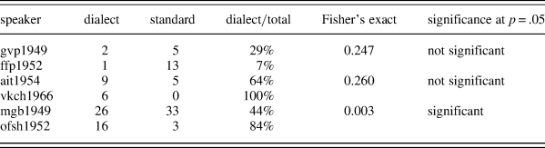
The figure suggests a consistent decrease in dialectal realization, with some variation in the middle generation. However, this intuitive reading is problematic, since the data come from a corpus, with different numbers of occurrences of the variable, and not from an experiment where the number of occurrences may be controlled. Differences in percentages that seem visually compelling may fail standard statistical tests for significance. Table 1 shows comparisons of three pairs of speakers, indicated as unfilled circles in Figure 1. Only the last difference between mgb1949 and ofsh1952 is statistically significant. For the first and the second pair, the tacit assumption that the number of occurrences is high enough to ensure significance of differences is not borne out. In the next section, we use logistic regression models to add a statistically informed visualization of the trajectory of change.
Pairwise comparisons of realizations of PREP for six speakers

Logistic regression model
The binomial logistic regression model is a statistical model that represents the dependence between a set of independent variables, called predictors, and the probability of an event with a binary (hence binomial) outcome. It assumes a linear regression of log odds, that is, a unidirectional and, in a certain sense, constant rate of change in the probability of an event in time, assuming a change progressing from 0 to 1, or vice versa. In this paper, we study the relation between the scalar value of age as a predictor and the probability of dialectal realizations in speakers as the target variable. The data input to the model are the observations of dialectal and standard realizations of a variable by a speaker, for all speakers. Crucially, the impact of an individual speaker to the model depends on sample size.
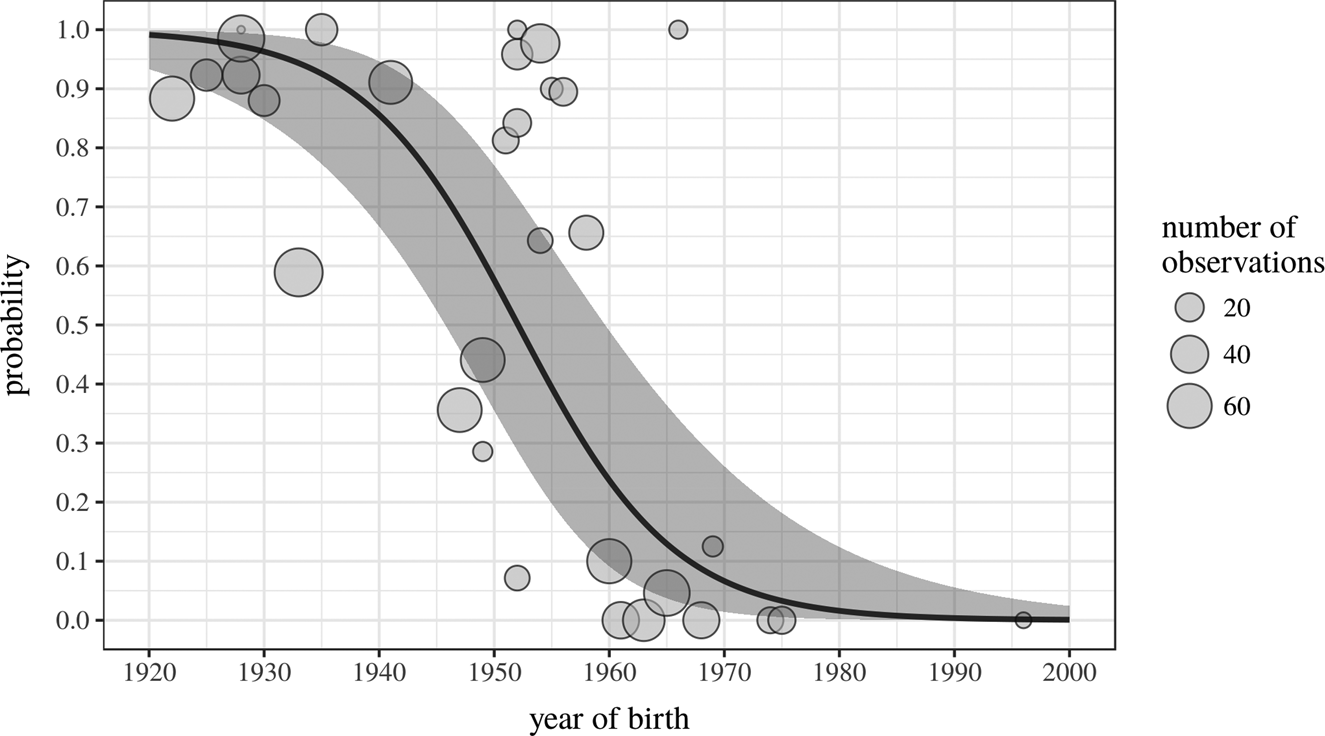
The probability of dialectal realization may vary strongly among speakers of a similar age (cf., for example, Figure 1 above): some are ahead of their age peers, others lag behind. To account for such differences, we use a mixed-effects logistic regression model with speaker as a random effect (see Baayen, Reference Baayen2008:271 ff.). The model expects the probabilities with speakers in a specific age to group around a certain central value. Assuming that a stronger individual deviation is less expected than a weaker deviation, the mixed-effects model traces the change of this central value over time. The model was fitted using the R library lme4 (Bates, Maechler, Bolker, & Walker, Reference Bates, Maechler, Bolker and Walker2015), and the graphs plotted with ggplot2 (Wickham, Reference Wickham2016). Figure 2 shows the expected probability of dialectal realization as a function of time for the PREP variable (absence of /nʲ/ after preposition) discussed in the previous section.
PREP variable: logistic regression model with speakers as random effect.

Figure 2 shows that there is a decrease in the dialectal realization of PREP over time by displaying the logit curve that best fits the data. The shaded area shows the confidence interval, that is, it shows possible curves at a confidence level of 0.95. Similar charts for the other variables indicate that all the observed dialect features show a clear tendency to wane in younger speakers (see the online appendix, Figures A1 to A11).
To estimate the statistical significance of the logit regression model, we used ANOVA to compare the model that uses the year of birth as a predictor and the model that does not use it. In other words, we tested whether the model that allows for change over time is better than the model that assumes absence of change over time (suggesting that the probability of dialect versus standard realization for a speaker is independent of her age). For all variables, the comparison shows a high level of statistical significance (see ANOVA line in Table A1 in the online Appendix). In all variables except TU, the p-value is less than 0.001. For TU, it is less than 0.01.
Logistic regression as a tool of cross-variable comparison: initial level, steepness, and turning point
Logistic regression models are a standard way to detect the correlation of a set of observations of a binary variable with a predictor such as age. We now use logistic regression to compare the rates of dialect-to-standard convergence of all variables, starting with a visual analysis to then motivate numerical parameters of change.
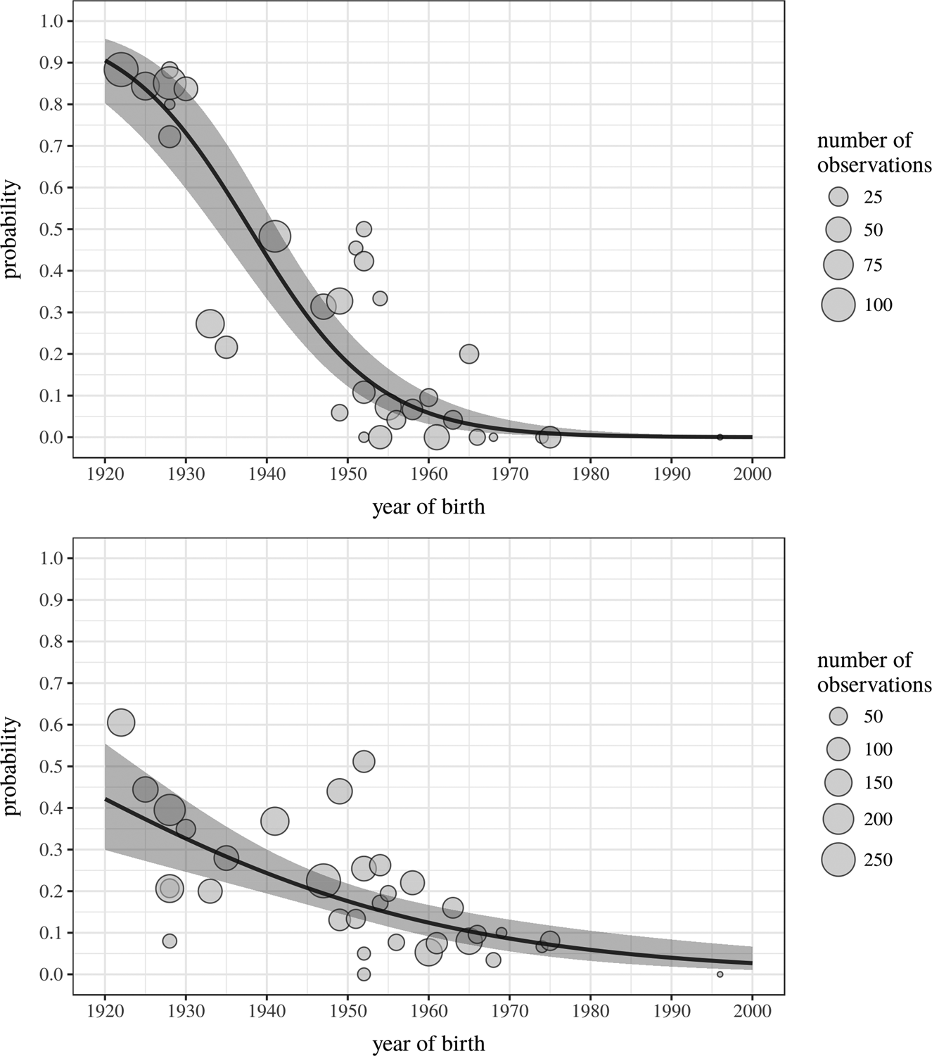
Figure 3 shows the variables OT (realization of the particle after consonants) and ADJ (contraction of adjectival ending).
Logistic regression charts: variables as function of age with speakers as random effect of OT (realization of the particle after consonants, above) and ADJ (contraction of adjectival ending, below).

The charts reveal several visual differences between the two variables. The ADJ curve starts lower than the OT curve; in other words, the loss of the ADJ variable is more advanced in the oldest cohort. We call this the initial level. Second, the OT curve goes down much steeper than the ADJ curve; in other words, the change is more abrupt. We call this steepness. Finally, the two curves cross the level of y = 0.5 in different places, that is, indicating different values for the age group in which the probability of the standard realization equals the probability of the dialectal realization. We call this the turning point. Footnote 5 For ADJ, this point falls well before our data start, while for OT it is around 1940.
Each of the three characteristics initial level, steepness, and turning point are indicative of the rate of change. They are not independent (see below); but, while comparing individual variables, some of these indicators of the rate of change may be more discriminative than others.
We now relate these properties to quantitative parameters of the curve. The two first characteristics correspond to two standard parameters of a logistic regression model, its b0 and b1 coefficients, respectively. These two coefficients fully determine the form of the curve. The greater the b1 coefficient, the steeper the curve. For the initial level, instead of the b0 coefficient (the intercept), which is difficult to interpret in qualitative terms, we use the probability p0 of dialectal realization predicted by the logistic model for our oldest speakers, that is, those born in 1920. This is the value of the logistic function for 1920, calculated as p0 = eb0 / (1 + eb0).
Any logistic model has a certain level of uncertainty depending on its input. Rather than exact values, it provides intervals within which the values of p0 and b1 lie at a certain level of confidence. In order to compare variables, we thus have to compare the intervals in which the values of the logistic model parameters lie with a confidence level of p > 0.95. If the intervals for the value of a parameter do not overlap, the variables under comparison are considered statistically different in respect to this parameter (see Baayen, Reference Baayen2008:131 ff.).
The turning point, finally, is the year where the regression line crosses a dialectal realization value of 0.5. Determining the confidence interval for this value is less straightforward. We define it as the interval between the first and the last year of birth in which a probability of dialectal realization of 0.5 is included in the confidence interval, that is, the years where the shaded area includes the level of 0.5.
Table 2 corresponds to our comparison of the two logistic curves.Footnote 6 The confidence interval for the initial level of ADJ is lower than of that of OT, and the two do not overlap; in other words, dialect preservation in old speakers for ADJ is lower. The steepness values of OT are higher than that of ADJ; in other words, the change is more abrupt. The turning point is reached by ADJ much earlier, before 1923, and the interval does not overlap with the turning point interval of OT (starting from 1934).
Comparison of (OT) and (ADJ) variables

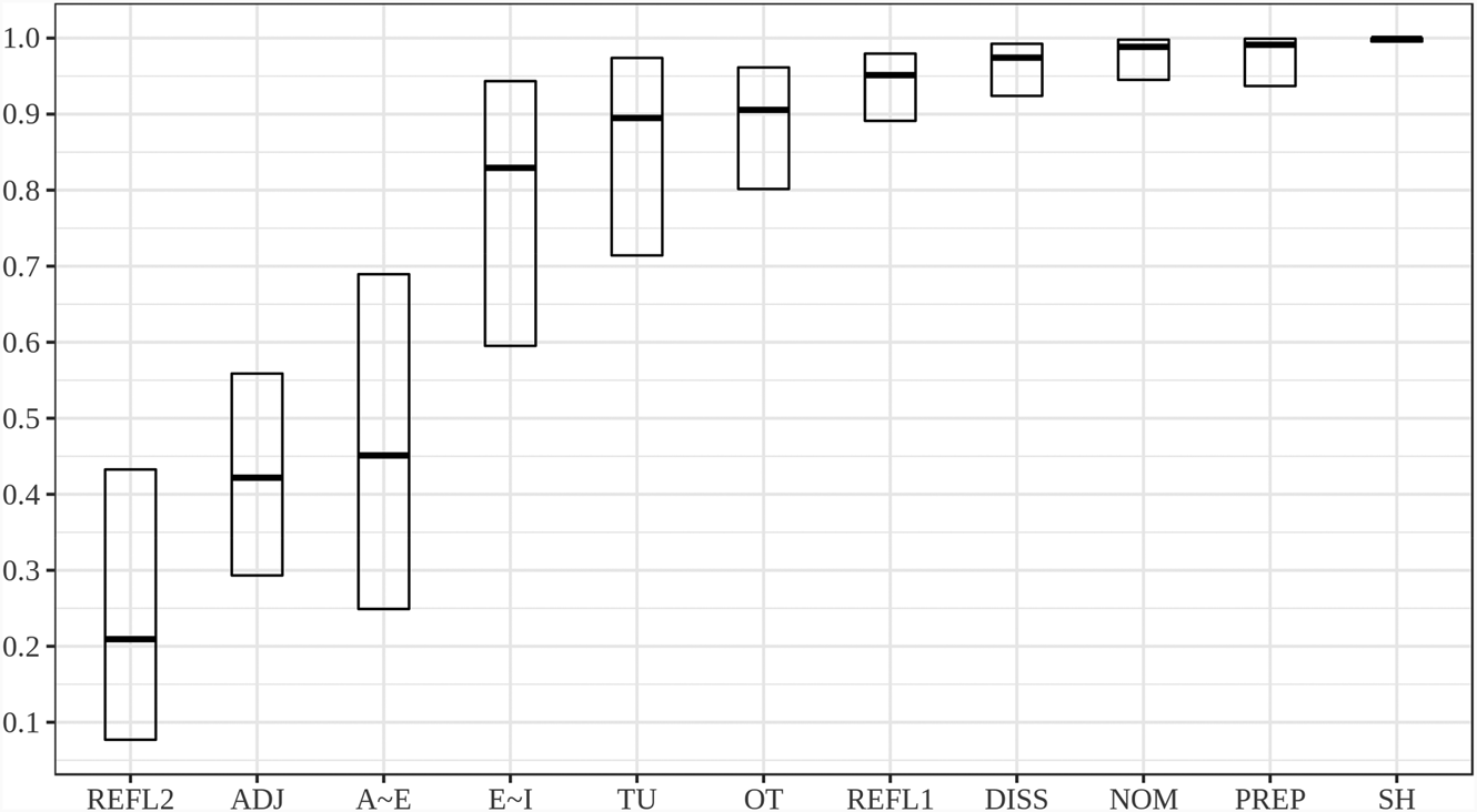
We now can compare the logistic models numerically for all variables: Figure 4 shows the variables ordered in terms of their initial level, Figure 5 in terms of their steepness, and Figure 6 in terms of the turning point of change.
The initial level parameter (p0). Lower values indicate lower dialect retention in our oldest speakers.

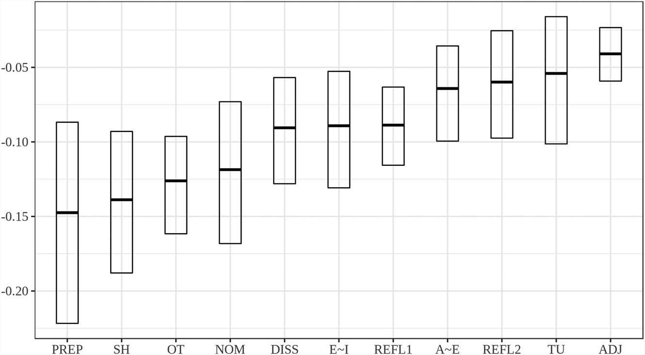
The steepness parameter (b1). Higher values indicate flatter (less steep) change.

Turning point values (probability of dialectal and standard realization equal at 0.5 by year of birth).

In the next section, we discuss possible interpretations of the differences between the variables.
DISCUSSION
We now discuss our variables and compare them in light of the model and the parameters we have defined above.
There are some obvious properties that should be noted. First, given that all dialectal variables are lost by the end of the twentieth century, any change that starts late and at a high dialectal level must be steep. Similarly, a change that starts at a low level of dialectal realizations must take a rather flat trajectory. Furthermore, the model assumes a change from a nearly exclusive use of the dialectal realization at some point in the past. This means that, for variables that do not show a high rate of dialectal realizations in our data, the model assumes such a state in the time well before our observations with a very early turning point. We will see below that these assumptions may not always be warranted.
Initial level
As Figure 4 shows, three variables start at low initial levels of dialectal realization with less than 0.5 probability even with our oldest speakers, born in the 1920s: ADJ (adjective contraction), REFL2 (reflexive vowel retention), and A~E (a-raising). These low levels are confirmed by dialect atlas data (DARJA; see below) from the 1950s that report inconsistency of dialectal realization for these three variables in villages close to ours (4 and 25 km, respectively) with speakers born in the last quarter of the nineteenth century. We suggest that this is primarily due to characteristics of the base dialect rather than from early convergence to the standard.
Concerning REFL2 (reflexive vowel retention), a general tendency to not fully preserve the final vowel of the reflexive morpheme after verb-final vowels is attested across a majority of the Russian dialects covered in DARJA (II, map 104). It is quite plausible to assume that this tendency had been reflected in some yet unknown pattern of facultative or context-conditioned realization of the reflexive vowel in the base dialect before convergence to the standard started to play a role.
Concerning ADJ, variation between the full and contracted form of the adjective as well as other VjV-sequences is characteristic of the Vologda dialects to which the Mikhalevskaya dialect belongs. This distinctive feature of Vologda dialects, together with Kostroma dialects, sets them apart from other regions where the contraction of VjV is obligatory (DARJA II, maps 53–56, 87–90; Orlova, Reference Orlova and Orlova1970:168–177). Again, a plausible interpretation of the early variation is that this is due to dialect-internal development rather than to early influence by the standard. Otherwise, it would be difficult to explain the observed areal constraint to the Vologda and Kostroma dialects.
Finally, for A~E, an early decline can be attributed to analogical change. The DARJA (I, map 41, and II, maps 58–59) data from the 1950s for speakers born between 1880 and 1916 show that, in the northeastern Vologda dialect region (to which Mikhalevskaya belongs), /a/ was not raised to /e/ in the morphological endings of the instrumental -/amʲi/ and comparative -/aje/ regardless of whether the preceding consonant is palatalized; this has also been observed for -/aje/ in the seventeenth to nineteenth centuries by Bromley (Reference Bromley and Bromley2002:591–593). It is unclear whether, in these morphological contexts, the raising ever occurred in the dialect. In both the dialect atlas as well as in the data from our oldest speakers, this alternation is already restricted to certain lexical roots and thematic -a- in the verbal paradigm. These are indications that an analogical change that would reverse raising may have started prior to extensive contact with the standard, and, in combination with the pressure of the standard language, led to an early decline in lexemes that exhibit it.
We conclude that, for all three variables, the low initial level of dialectal realization returned by the logistic regression model could be, to a large part, due to the presence of variation in the base dialect itself. The apparent early loss can be best explained by system-internal factors, rather than by an influence of the standard that exhibited a stronger or earlier influence on these than on other variables.
Turning to the remaining nine variables, we see that they by and large form a group whose rate of dialectal realizations, in our oldest speakers, is above 80 percent. Note that E~I (yat-raising) as well as TU and OT (postpositional particle) seem to have somewhat lower levels than the others. DARJA shows earlier variation with E/I already for speakers born in the nineteenth century, so there is some evidence that this change, too, had already started in the base dialect (but probably did not, in contrast with the otherwise similar A~E variable, develop morphological conditioning). However, our data are not conclusive.
On the high end, SH (retroflex sibilant) stands out with almost exclusive dialectal realizations and, due to a large number of occurrences, a narrow confidence interval; we will return to this variable below.
Given the above considerations concerning the other three variables that have lower initial levels, we can conclude that the dialect was not yet strongly influenced by the standard in the oldest cohort, even though some minor degree of influence can be assumed. Some of the observed variation may also be due to lifespan change (see discussion below). It is in later years that the influence from the standard clearly becomes the decisive factor of linguistic variation.
Turning point
The second parameter we consider is the turning point, that is, the year of birth of those speakers who are equally likely to use the dialectal and the standard realization of a variable (see Figure 6). The three variables with low initial level (ADJ, А~Е, and REFL2) are estimated to reach this point prior to our observations. As argued in the previous section, these variables might have shown stable variation already in the base dialect, which calls the reconstructed early turning point into question.
Aside from these three variables with very early turning points, we have two more groups. First, we have E/I (yat-raising) and OT (the -/ot/ allomorph of the postpositional particle); these reach the turning point already in the generation born in the 1930s or early 1940s. A further group consists of five variables with overlapping intervals, their turning point falling between the 1950s and the 1960s. These include PREP (/nʲ/ after preposition), REFL1 (reflexive vowel quality), NOM (pronominal nominative plural), DISS (dissimilation of /kt/), and SH (retroflex sibilant). REFL1 is similar to PREP, and DISS is similar to NOM. As with the initial level, SH (retroflex sibilant) stands out, since it reaches the turning point very late (certainly later than the early 1960s) so that its interval does not intersect with two of this last group, PREP and REFL1. Finally, TU (postpositional particle) has a very wide interval; in other words, for this variable, the turning point parameter is not discriminative enough in our data.
We see that closely related variables with similarly high initial levels may have rather different turning points. This is most conspicuous with TU and OT, variables both relating to allomorphs of the postposed particle; we will return to these variables below.
Steepness
The third parameter, steepness, is not very discriminatory for our data. Figure 5 shows that the intervals of almost all variables are quite wide and all overlap to some extent, with the sole exclusion of ADJ (adjective contraction), which is set apart from PREP, SH, OT, NOM, and REFL1 by virtue of its high value, that is, flat trajectory. Recall that this variable was most probably not at 100 percent in the base dialect.
Guided by the best-fitting models (bold horizontal lines), we can observe that, among the group of four flat variables, all except TU (-/tu/ allomorph of postpositional particle) have a very low initial level to begin with, which explains the flat trajectory in a trivial way.
A closer look at SH and TU
In this section, we single out two variables that emerge as divergent from the others in the analysis above.
SH (retroflex sibilant) stands out. It has, with a narrow confidence interval, the highest initial level of all at close to 100 percent. It reaches the turning point very late, in the 1970s. As the inspection of the graph reveals, most speakers seem to be rather categorical for a long time, before an extremely steep decline in dialectal realizations takes place.
This effect of abruptness of change is partly due to our operationalization. The phonetic inventory of our oldest speakers actually includes two positionally distributed variants, [ʂt͡ʂ] and [ʂː], which we conflate in order to define a binary variable opposing dialectal versus standard realizations. The change to the standard [ʃʲː] takes place in two phases (Ignatenko, Reference Ignatenko2015) that is obscured by our model. First, the [ʂː] variant replaces [ʂt͡ʂ] and then changes to the standard realization [ʃʲ]. Basically, this is a chain shift [ʂt͡ʂ] → [ʂː] → [ʃʲ]. Conflating [ʂt͡ʂ] and [ʂː] in a single value of ‘dialectal realization,’ a necessary step toward a logistic regression model, made the first phase of the shift invisible. In the particular case of SH, the long retention of dialectal realizations and subsequent abrupt change can be partly attributed to our modeling of the data. This highlights a limit of our approach.
Secondly, we single out TU, which behaves remarkably differently from OT, the other allomorph of the same particle. TU and OT start at similarly high initial levels. Then, OT diminishes quite quickly and consistently, while TU continues to be used at comparatively high levels, with, however, large variance among speakers. This leads it to have very flat trajectory; in terms of steepness, it is grouped with the three variables that have low initial levels, that is, ADJ (adjective contraction), REFL2 (reflexive vowel retention), and А~Е (a-raising). In terms of turning point, however, it patterns together with a different set of variables but has an exceptionally large confidence interval due to the wide variance between speakers.
The difference with OT, which is lost early and fast, is conspicuous. We see this as linked to its linguistic nature (see the Variables section above): while -/tu/ is different from standard -/to/ only in the (unstressed) vowel, -/ot/ has a very different phonological structure. It is probably more salient as a characteristic of village speech, and, we argue, thus more prone to be dropped given the low prestige of the dialect. We return to the notion of salience in explaining different rates of variables below.
SH and fudge realizations in Kochetov (Reference Kochetov2006)
Our observations related to SH above are different from those provided in Kochetov's (Reference Kochetov2006) study of dialect loss in a small town in the Perm region (North Urals). Kochetov compared the variable SH to okanje, that is, the realization of unstressed /o/ as [o] in the dialect, as opposed to standard Russian, where unstressed /o/ and /a/ are merged. The dialectal realization of SH is completely lost by Kochetov's speakers already in the generation born shortly after World War II. Okanje, in contrast, first drastically decreases but then stabilizes at an intermediate level in the 1960s and is subsequently retained. Kochetov explains the contrast between the two variables in terms of salience. He argues that the difference between the two realizations of SH, on the one hand, is salient, because it involves two distinct articulatory gestures that do not allow for intermediate realizations. The realization of unstressed /o/ as [o] or [a], on the other hand, allows for an intermediate realization, [ɔ]. The latter serves as a “fudge”’ between the dialect and the standard (Chambers & Trudgill, Reference Chambers and Trudgill1998:110 ff.). He argues that such a “fudge” variant is not available for SH, and for this reason the change is complete (Kochetov, Reference Kochetov2006:115 f).
Kochetov's explanation is incompatible with our findings. As discussed above, for SH we observe a shift from the dialectal retroflex [ʂt͡ʂ] first to the intermediate stage of [ʂː] and only then to the standard palato-alveolar [ʃʲː]. This intermediate stage looks very much like a “fudge.” However, it does not stabilize in our data; rather, it is lost quickly in the generation born in the 1960s.
All variables except for PREP (absence of /nʲ/ after preposition) and OT (-/ot/ allomorph of the postpositional particle) arguably allow for intermediate realizations, and we have indeed observed them with some variables, including those outside the scope of this paper (realization of affricates and nonpalatalized lateral /l/). What we do not observe is that any of these variables stabilize at such “fudge” realizations. Rather, they eventually converge with standard or regional variants.
Kochetov's stabilized “fudge” realization of okanje is probably better understood as a complete shift to the regional standard, which is different from the prescribed standard and represents an intermediate variant ([ɔ] rather than standard [a] or dialect [o]) that has stabilized on a regional level (as Kochetov himself notes [Reference Kochetov2006:115]). Such regiolectal variants are, in our view, of prime importance for an adequate understanding of dialect change in Russia.
Factors in different rates of convergence
Ultimately, we seek to understand factors that play a role in different rates of retention of our variables. One such factor is perceptual salience: given its low prestige, variables that are seen to be emblematic of the dialect are lost earlier, while variables that are less readily noticed are lost later.
To see this, consider the group of six variables with the latest turning points in Figure 6 above. Comparing them to the group of variables with early turning points (excluding REFL2 and ADJ, which probably never had 100 percent of dialectal realizations [see the Initial level section above]), we see that those variables that are lost early involve changes in stressed root vowels and segmental phonology and/or are morphophonologically conditioned: E/I (yat-raising), A/E (a-raising), OT (-/ot/ allomorph). Among those that persist longer, we see, in contrast, variables that show no change on the phonological level (SH, retroflex sibilant) or involve unstressed final vowels such as REFL1 (reflexive vowel quality) and TU. We thus see some evidence that more (morpho)phonologically salient features of our dialect are lost earlier than less salient ones.
A salience-based explanation is also plausible for ADJ, which probably initially involved a pragmatically conditioned alternation between full, hiatic, and contracted realizations of the adjectival еnding /aja/: [aja]~[aa]~[a]. This is easily perceived as a characteristic of rapid speech and thus little salient; it persists to some degree in the speech of our youngest speakers.
However, there are also problematic cases in our own data: NOM (pronominal nominative plural) is a clearly morphophonologically defined variable concerning a vowel in stressed position, yet it is lost late.
Generally, salience is notoriously difficult to operationalize in a noncircular fashion, and phonemic status of variants is often far from clear. For example, it is difficult to decide whether the variable DISS (dissimilation of [kt] to [xt]) concerns the use of a different phoneme or of a positional variant. In any case, we would intuitively not rate this variable as particularly salient, as this dissimilation is articulatorily simple and widely attested, which fits well with the observation that DISS is lost very late.
An important factor in the persistence of dialectal variants is their presence in other regionally or socially defined varieties of Russian. DISS is a case in point: it is widespread in many varieties of Russian, presumably including the local regiolect toward which our dialect is converging, as well as substandard urban colloquial registers all over Russia. The same can be said for REFL2 (reflexive vowel retention). REFL1 (reflexive vowel quality) can probably be considered part of the regiolectal variety of Russian with which the dialect is converging and is used in our data by a speaker born as recently as the 1990s. Above, we have argued that the persistence of okanje in Kochetov's (Reference Kochetov2006) study is likewise linked to its persistence in the regional urban variety of Russian.
We thus see at least two different factors at work. First, perceptual salience of a variable is important in influencing its rate of change: the more noticeable and emblematic of the dialect, the quicker a variable gets discarded; OT is a case in point. A second factor is presence of a variable in other nonstandard varieties as perceived and negotiated by the community—be they socially or regionally defined. The persistence of REFL2 or DISS in our dialect are best explained by this factor. These two factors do not necessarily contradict each other: very salient features are hardly expected to survive in the regional standard, for example.
LIMITS OF THE PROPOSED MODEL
In this section, we review limitations of using logistic regression models for the comparison of variables in apparent time studies such as presented here.
The impact of lifespan change
According to a large range of literature (e.g., Bowie & Yaeger-Dror, Reference Bowie, Yaeger-Dror, Honeybone and Salmons2014; Fruehwald, Reference Fruehwald2017; Labov et al., Reference Labov, Rosenfelder and Fruehwald2013; Sankoff & Blondeau, Reference Sankoff and Blondeau2007), lifespan change can lead to underestimation of the rate of change. However, while lifespan changes can differ strongly across variables and speakers (but see discussion in Labov [Reference Labov2001]), they are generally not seen to be strong enough to undermine the results of apparent time studies.
In respect to our method of comparing variables, however, the effect of lifespan change may be decisive. Even relatively small lifespan changes may either obscure actual differences or, on the contrary, introduce apparent differences which are not actually there. For instance, the fact that the confidence interval for the initial level does not overlap for REFL2 (reflexive vowel retention) and E~I (yat-raising) may be due to actual differences in the retention of these variables in the dialect when our oldest speakers were young. On the other hand, it may, to a certain extent, be due to different rates of lifespan change that make these variables less similar in the speech of these speakers as observed today than they used to be in their youth. This does not contradict the general view that the effect of lifespan change is not strong enough to undermine the apparent time method. Rather, this effect may undermine the statistical significance of differences between variables the way we measure them. Even a small impact from the presence of lifespan change may make such differences insignificant, especially for those variables whose confidence intervals are very close but do not overlap. At this point, we see no way to resolve this methodological problem.
Assumptions of the model
Other problems are linked to the nature of the model we use.
In an attempt to account for variation across speakers of the same age group, the mixed effects model assumes a normal distribution of the data with respect to random effects. In other words, the probability of dialectal realization is assumed to be normally distributed across speakers. This assumption is anything but obvious. It is probable that, at least for some variables, speakers of roughly the same age form two groups (a bimodal distribution), for example, in the period of the abrupt change. This is clear in the case of SH (see Figure A3 in the online appendix). Around 1960, most speakers are nearly categorical users of one of the two variants.
No less importantly, the limitation of the logistic regression model is that it makes assumptions about the dynamics of change. Logistic regression is used as a default hypothesis of a correlation between a factor and a probability of a binary outcome, similarly to how linear regression is used as a default hypothesis of correlation between a factor and a real number value. Both show that there is a statistically significant change in time (as opposed to the null hypothesis of absence of change), but do not necessarily reflect its dynamics. Problems with the application of linear regression models to change in progress are discussed in Fruehwald (Reference Fruehwald2017), who notes that language change does not have to be linear. He refers to Labov et al.’s (Reference Labov, Rosenfelder and Fruehwald2013) study of vowel shift in Philadelphia that shows changes in different directions at different points in the twentieth century. Obviously, if the change does not have to be unidirectional, it does not have to be linear (even if unidirectional), either. In other words, language does not (have to) change with at a constant rate.
The very same applies to logistic regression models. Logistic regression is an analytic derivative of linear regression (Hosmer & Lemeshow, Reference Hosmer and Lemeshow2000:6). In a certain sense, it also assumes a constant rate of change (roughly, the constant rate of change of the chance to get a particular realization of a variable). One consequence of this assumption is that a logistic curve is always symmetrical with respect to the point where it equals 0.5.Footnote 7 This symmetry is not based on empirical evidence but follows from the assumption of a constant rate of change. For the three variables with low initial levels, ADJ, A~E, and REFL2, our data suggest that the loss of what we consider to be a dialectal realization may be a combined effect of an early dialect-internal development and subsequent growing pressure from the standard (see the Initial level section above). Here, the loss is an amalgamation of two independent processes, and no linearity can be assumed.
Consider again Figure A3 for SH (retroflex sibilant) in the online appendix. What we see is an abrupt change, a leap from an almost categorical dialectal realization in the speakers born before 1960s to an almost categorical standard realization in speakers born after that. Contrary to the prediction of the model as visualized by the logistic curve, the change is very small, if present at all, before and after this period and very abrupt within it. For this variable, turning point (the years of birth of speakers who use dialectal and standard realization with equal probability) is a mere abstraction. Virtually all speakers are nearly categorical users of one or the other variant. Still, in terms of statistical tests (see Table A1 in the online appendix), the logistic regression model for SH performs well. This happens because the performance of the logistic model is compared to the performance of the zero hypothesis of the absence of change, an obvious strawman. Logistic regression is not a good approximation of the real dynamics of change.
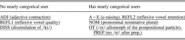
Looking at (non)categorical users may provide insights that are overlooked by the logistic regression model. Consider the following grouping of variables. Within each line of Table 3, the variables are more or less similar to each other in terms of the three parameters that we introduced above. However, as with Figure A1 to A11 in the online appendix, the variables on the right have some nearly categorical users of the standard realization. No such speakers are available for the variables on the left.
Availability of categorical users of a variable

The reason why only some new variants are adopted wholesale by some speakers may be due to perceptual salience, dialect awareness, and perceived emblematicity of certain realizations. Our model, however, cannot account for this issue. Because logistic regression assumes a constant rate of change of log odds, it simply cannot accommodate predicted rates of zero or 100 percent of dialectal realization, no matter the observed data. It therefore does not distinguish variables where some speakers are categorical from those where no such speakers exist.
CONCLUSIONS
Using data from the Ustja River Basin Corpus containing biographical interviews with inhabitants of a North Russian village, we have shown how logistic regression models can be used with corpus data not only to detect a clear correlation of dialect loss with year of birth but also to compare the rate of change across variables. We defined three parameters to model differences in the dynamics of change: initial level of dialectal realization of our oldest speakers, steepness of change, and turning point where speakers tend to show equal probability of using either the dialect or the standard variant. Although these parameters of change are not independent, they are not mechanically connected, either. We show how these parameters can be used to compare variables in a principled and informative way.
We also note that, in the case of some variables, users completely shift to the standard variant, while in the case of others the dialectal variant survives, even if marginally, a difference that is not captured by the logistic regression model. We tentatively link this to two possible factors.
First, we discuss an interpretation of differences between variables in terms of their different perceptual salience. In our data, the most persistent variables are those that do not involve phonological change (e.g., a chain shift [ʂt͡ʂ] → [ʂː] → [ʃʲ]), or those that occur in phonologically weaker positions (like the reflexive REFL1 or the particle TU, both postposed clitics). Other variables are perceptually more salient as they involve a phonological contrast or are morphologically conditioned, such as PREP, A~E, and E~I. It is these variables that acquire categorical users of the standard. We propose that perceptual salience is important in dialect awareness as a result of the social negotiation of specific variables, a hypothesis to be substantiated in future work.
A second factor we discuss is the presence of the dialectal realizations in other, regionally or socially defined, varieties of Russian. For example, the variable DISS (dissimilation of [kt] as [xt]) does involve a phonological contrast, but, unlike the above variables, in our data it never acquires categorical users of the standard variant. We suppose that perceptual salience is converted into emblematicity as a result of social negotiations of specific variables. In the case of DISS, emblematicity is probably weakened by the fact that this variant is common to substandard Russian. We adduce similar arguments in respect to other variables. Generally, in order to assess changes of the local dialects, we stress the need to take into account the bigger picture of variation in the standard language as it presents itself to the local speech community. Here, much empirical work on Russian still needs to be done (see Erofeeva, Reference Erofeeva2005).
Finally, Fruehwald noted that “the great benefit of linear models is that there is a very simple decision procedure to determine whether there is a change in progress” (Fruehwald, Reference Fruehwald2017:12). Mutatis mutandis, the same applies to logistic regression models. An important advantage of logistic regression as compared to other statistical models is that it takes into account the amount of data available from different speakers: speakers who provide less data have less impact on the model. It is thus well adapted to the analysis of corpus data. But while accepting logistic regression model as a default model and a means to detect language change, other more complex and more empirically oriented models are needed to assess the rate of change, such as generalized additive models as used in Labov et al. (Reference Labov, Rosenfelder and Fruehwald2013).
We thus argue that logistic regression models are a good tool to study language change only in a first approximation. They are imprecise as a tool to model its exact dynamics, because their assumption of a constant rate of change (of log odds), comparable to the assumption of linearity of change in linear regression models, is not entailed by anything we know about language change. Logistic regression models are therefore ultimately untenable as models of sociolinguistic change.
SUPPLEMENTARY MATERIALS
To view supplementary material for the article, please visit https://doi.org/10.1017/S0954394519000243.