1. Introduction
Especially since WWII, the carbon dioxide (CO2) emission level has risen due to militarization and economic growth around the world, and thus the level of CO2 emissions has approached the ceiling of CO2 emissions in the atmosphere at which environmental degradation will be irreversible. The level of CO2 emissions throughout the world was 32.1 billion tons in 2015, remaining essentially flat since 2013 (IEA, 2016). Energy-related CO2 emissions increased by 5,406 MMmt in the year 2014 (EIA, 2015).
Except for the years of major recession between 2007 and 2009, after an average annual increase of CO2 emissions of 3.8 per cent per year since 2003, the annual increase in the years 2012 and 2013 was at about half the level of the increases in the preceding decade. The main reason why emissions in the years 2012 and 2013 were smaller than predicted is due to the fact that economic growth in those years was below the annual average. In 2012 and 2013 the global economy grew at the level of 3.4 per cent and 3.1 per cent, respectively, while the average annual growth rate of GDP since 2003 is 3.9 per cent (IMF, 2014; Olivier et al., Reference Olivier, Janssens-Maenhout, Muntean and Peters2014). After 2013, in the US, CO2 emissions accounted for 82 per cent of all greenhouse gases (GHGs) from human activities. Human activities alter the carbon cycle by adding more CO2 emissions to the atmosphere. Moreover, they affect the ability of natural sinks to remove CO2 (US Department of State, 2007; NRC, 2010). And within the total increase in global CO2 emissions in 2013, there are remarkable differences among developed, emerging and developing countries (Olivier et al., Reference Olivier, Janssens-Maenhout, Muntean and Peters2014).
The link between militarization, CO2 emissions, economic growth and energy consumption is very important in this process. On the one hand, militarization affects CO2 emissions, economic growth and energy consumption; on the other hand, economic growth is supported by the relation between energy consumption and militarization. Thus the relationship between militarization, CO2 emissions, economic growth and energy consumption is complex and interrelated.Footnote 1
In this context, the main sources of CO2 emissions in G7 countries, especially in the United States, are economic growth and militarization. Industrial firms and facilities including hundreds of military bases overseas, as well as military equipment and vehicles, weapons and personnel, emit CO2 emissions. determined that the fossil fuel energy consumption from industrial output is only about 15 per cent of total US CO2 emissions and only 12 per cent of total US GHG emissions in 2013 (EPA, n.d.). The US army emitted more than 70 million tons of CO2 in 2014 (Neslen, Reference Neslen2015).
The institutions, technologies, weapons and behaviors of the military can produce ecological problems (Jorgenson and Clark, Reference Jorgenson and Clark2011). Militarization contributes to numerous forms of environmental pollution. The tests of atomic and nuclear bombs produce radioactive fallout expanding throughout the world (Commoner, Reference Commoner1967, Reference Commoner1971). The environmental effects of militarization are not limited to war, large-scale conflicts (Jorgenson, Reference Jorgenson2005; York, Reference York2008) and the testing of nuclear weapons and atomic and nuclear bombs (Jorgenson et al., Reference Jorgenson, Clark and Givens2012). Militarization causes further environmental pollution via energy consumption. The army's activities and related technologies require a great deal of energy consumption during its operations and maintenance of its infrastructure, troops and equipment. In the 1980s, a quarter of jet fuel consumption and approximately three-quarters of petroleum was consumed by the armed forces – by their vehicles, aircraft, sea vessels, other forms of warfare machinery, and so on (Renner, Reference Renner and Brown1991; Clark et al., Reference Clark, Jorgenson and Kentor2010).
While militarization and energy consumption tend to increase in a linear manner, environmental degradation is non-monotonic. The effects of environmental pollution are seen throughout the entire world. CO2 emissions are relatively greater in developed countries shaped by higher military expenditure (Rice, Reference Rice2007).
In this paper, CO2 emissions caused by militarization will be explored. Although the relationship between energy consumption, CO2 emissions and economic growth has been analyzed by numerous papers, the relationship between militarization and environmental pollution was analyzed in a few papers by environmental sociologists in the context of the ‘treadmill of destruction’ theory (Clark et al., Reference Clark, Jorgenson and Kentor2010; Jorgenson et al., Reference Jorgenson, Clark and Kentor2010, Reference Jorgenson, Clark and Givens2012; Givens, Reference Givens2014).
In the context of energy economics, Bildirici (Reference Bildirici2015) examined the dynamic relationship between economic growth, energy consumption and militarization in China for the period 1987–2013, using the autoregressive distributed lag (ARDL) method. She determined the short- and a long-run relationship between militarization, energy consumption and economic growth. The results of her paper implied that economic growth and energy consumption in China are based on militarization.
This study aims to analyze the causal relation among CO2 emissions, energy consumption, economic growth, and militarization in the G7 countries (Canada, France, Germany, Italy, Japan, the United Kingdom and the United States). This study is the first paper that attempts to analyze the potential relations between these variables, using panel cointegration and causality methods. Since the determination of a long-run relationship between the variables is very important for G7 countries' energy policy and strategy, we did not wish to depend upon only one testing methodology. The results obtained by this study are ensured by several tests. Within this approach, we examine whether the preponderance of the evidence makes a convincing case for robust evidence. In this paper, four steps were followed to establish a long-run and a causal relationship between the variables. At the first step, panel unit root tests were applied. Three unit root test were used, namely the Levin et al. (Reference Levin, Lin and Chu2002) test, the Im et al. (Reference Im, Pesaran and Shin2003) test and Pesaran's (Reference Pesaran2007) cross-sectionally augmented IPS test. At the second step, three cointegration tests, the Pedroni, Johansen and panel autoregressive distributed lag (PARDL), were applied. The Pedroni and Johansen tests allowed us to assess whether there is a long-run equilibrium relationship, but these tests do not provide parameter estimates either for the long run or for the short run. At the third step, in order to determine and control the robustness of the PARDL long-run estimators, two additional long-run estimators – the dynamic ordinary least squares (DOLS) developed by Stock and Watson (Reference Stock and Watson1993) and suggested by Kao (Reference Kao1999) and the fully modified ordinary least squares (FMOLS) developed by Phillips and Hansen (Reference Phillips and Hansen1990) and suggested by Pedroni (1996) – were employed. At the fourth step, to complement the results determined by panel cointegration methods, the panel trivariate causality test was carried out.
The remainder of the paper is organized as follows. The literature regarding militarization, energy consumption, CO2 emissions and economic growth is discussed in section 2. The relation between militarization, economic growth, CO2 emissions and energy consumption in the G7 countries is discussed in section 3. Data specifications are identified in section 4 and the econometric methodology is described in section 5. Section 6 covers the empirical results, and section 7 includes the conclusions and policy implications.
2. Literature review
Orthodox economic theory failed to consider environmental pollution. When energy is included in the production process, systemic disorder increases due to entropy. The environmental pollution caused by energy consumption is a result of energy degradation. But orthodox theory accepted that economic growth can solve environmental problems.
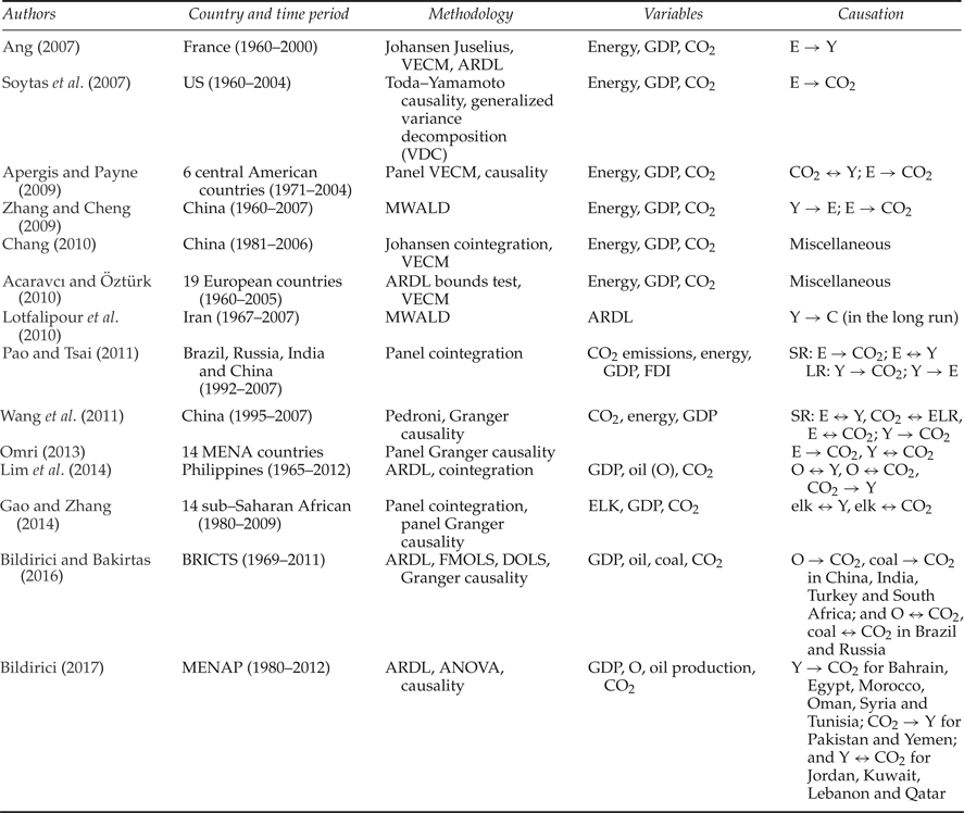
As a differentiation from an neoclassical economist's perspective, Meadows et al. (Reference Meadows, Meadows, Randers and Behrens1972) determined that economic growth has significant environmental impacts and the future world will collapse. The world economy will reach its physical limits in terms of fossil resources, population, agricultural production, industrial production, environmental pollution and consumption of non-renewable natural resources (Kaika and Zervas, Reference Kaika and Zervas2013). Furthermore, the relation between environmental problems and economic growth was analyzed by many papers with regard to the Environmental Kuznets Curve (EKC) hypothesis, following Grossman and Krueger (Reference Grossman and Krueger1991). Grossman and Krueger (Reference Grossman and Krueger1991, Reference Grossman and Krueger1995), Shafik and Bandyopadhyay (Reference Shafik and Bandyopadhyay1992), Shafik (Reference Shafik1994), Selden and Song (Reference Selden and Song1994), Tucker (Reference Tucker1995), Cole et al. (Reference Cole, Rayner and Bates1997) and De Bruyn et al. (Reference De Bruyn, van den Bergh and Opschoor1998) analyzed the inverted U-shaped EKC. Table 1 summarizes the literature addressing the causal link between energy consumption, CO2 emissions and economic growth.
CO2 emissions, energy consumption and GDP relation

Notes: Y denotes GDP.
The present literature generally focuses only on the relationship between energy consumption, CO2 emissions and economic growth and it accepts that energy consumption is one of most important reasons. However, not only economic growth, but also militarization affects environmental pollution. The majority of CO2 emissions originate from the phases of economic growth and militarization.
3. Militarization, economic growth and energy consumption in G7 countries
Environmental pollution is closely related to the G7 countries' economic growth, energy consumption and militarization, and especially the US's militarization and energy consumption. After the World Wars, new weapons capable of immense destruction changed warfare and affected the pace of militarization. While the army became more distinct, energy consumption and environmental pollution increased as a result of high-tech equipment and new weapons, especially the nuclear weapons developed by scientists.
As military supremacy has been very important since the second half of the 20th century, scientists and engineers turned their research focus toward addressing the technological needs of the military. In addition to this, the expansionary dynamics of militarism produced specific forms of environmental degradation. Nowadays militarization continues under the impact of technological advances, infrastructural development, geopolitical competition and growth in troop size. Military powers cause environmental degradation by their military equipment, tests of nuclear bombs, military bases, weapons production and war (Hooks and Smith, Reference Hooks and Smith2004, Reference Hooks and Smith2005; Jorgenson et al., Reference Jorgenson, Clark and Kentor2010; Clark and Jorgenson, Reference Clark, Jorgenson and Ritzer2012).
Warfare in the last half of the 20th century and first half of the 21st century differs with regard to its use of technological weapons, the lethality of weaponry and the scope of environmental devastation (Hooks and Smith, Reference Hooks and Smith2005). The Center for Disarmament estimated that global military operations utilized aluminum, copper, nickel and platinum which contribute to environmental pollution (Renner, Reference Renner and Brown1991). During the six weeks of the 1991 Persian Gulf air war, more weapons were used than during the protracted Vietnam War (Levy et al., Reference Levy, Shahi, Lee, Levy and Sidel2000). According to US Army estimates, during the first three weeks of war in Iraq in 2003, 40 million gallons of fuel were consumed (Sanders, Reference Sanders2009). Moreover, the Pentagon, for example, accounted for 93 per cent of the fuel consumption of the US government in 2007 (Air Force: 52 per cent; Navy: 33 per cent; Army: 7 per cent; other DoD: 1 per cent) (Lengyel, Reference Lengyel2007).
The defense industry and department of the G7 countries consumes large amounts of energy in planes, ships and tanks. Even in peacetime, military institutions and their activities consume vast amounts of fossil energy for research and development, maintenance and operation of the overall infrastructure. Capital-intensive militaries in the G7 countries employ equipment, personnel and advanced weaponry that require an enormous amount of fossil fuel energy to facilitate the rapid movement of troops. Furthermore, in the G7 countries, the Department of Defense consumes more energy than any other organization in the world. The energy consumption of the military causes environmental pollution via the effects of various toxins and chemicals involved in the use of dangerous weapons.
The above-mentioned effects of militarization are further magnified by the testing of nuclear weapons and atomic and nuclear bombs. Therefore, even without the existence of any war, the defense sector consumes huge amounts of fossil fuel energy.
4. Data specifications
The annual data used in this study cover the period from 1985 to 2015 for Canada, France, Germany, Italy, Japan, the United Kingdom and the United States. The energy consumption (c), defense expenditure (m) as a measure of militarization, CO2 emissions as a measure of environmental pollution (co), and real per capita GDP (y) are used as variables. In order to minimize skewness, all variables were measured in natural logarithms.
The data on energy consumption were taken from the World Bank and BP statistics. Defense expenditure was measured in constant 2005 US dollars and obtained from the World Bank. Defense expenditure data comprise all current capital expenditures. Real per capita GDP data were obtained from the World Bank and the International Financial Statistics of the IMF. CO2 emissions data were taken from World Bank statistics which represent the total CO2 emissions from fossil fuels in 1,000 metric tons for the 1985–2015 period.
5. Econometric methodology
As the first stage, three panel unit root tests – the Levin et al. (Reference Levin, Lin and Chu2002) test, hereafter referred to as the LLC test; the Im et al. (Reference Im, Pesaran and Shin2003) test, hereafter referred to as the IPS test; and Pesaran's (Reference Pesaran2007) cross-sectionally augmented IPS test, hereafter referred to as the CIPS – are used in this study. At the second stage, three panel cointegration tests – the Pedroni, Johansen and panel ARDL tests – are used. At the third stage, the FMOLS and DOLS methods were applied. Pedroni's (Reference Pedroni1999) methodology allows us to test for the presence of cointegration, but it does not provide an estimation of a long-run relationship. Pedroni (1996) suggests a FMOLS estimator to obtain the panel data estimates. At the fourth stage, panel causality tests were applied to determine the causal relation. The panel trivariate Granger causality test was preferred.
5.1. Panel unit root tests
The LLC test, the IPS test and the CIPS tests were used. While the LLC test depends on pooled data, the IPS test is obtained as an average of augmented Dickey–Fuller (ADF) test statistics. The LLC panel unit root test is based on the following equation:
 $$y_{it}=\rho_{i}y_{i\comma t-1}+z^{\prime}_{it}\gamma +u_{it}\comma \; \quad i= 1\comma \; \ldots \comma \; \quad N\semicolon \; t = 1\comma \; \ldots\comma \; T\comma \;$$
where z
it
can be a fixed effect or time trend as well as a constant like zero and 1. The LLC test assumes that residuals are independently and identically distributed with mean zero and variance
 $\sigma_{u}^{2}$
and ρ
i
= ρ for all values of i. The null hypothesis can be constructed as H
0: ρ = 1 and the alternative, H
1:ρ < 1, means that all series are stationary. The t-statistic is:
 $$t_p =\displaystyle{{\lpar \hat{\rho}-1\rpar \sqrt{\sum\nolimits_{i=1}^N {\sum\nolimits_{t=1}^T {\tilde{y}_{i\comma t-1}^2}}}} \over {\displaystyle{{1}\over{NT}}\sum\nolimits_{i=1}^N {\sum\nolimits_{t=1}^T {\tilde{u}_{it}^2}}}}$$
and
 $$s_e^2 =\displaystyle{{1}\over{NT}}\sum_{i=1}^N {\sum_{t=1}^T {\tilde{u}_{it}^2}}.$$
The IPS unit root test can be specified as:
 $$y_{it}=\rho_{i}y_{i\comma t-1}+\sum_{j=1}^{p_i}\varphi_{ij}\Delta y_{i\comma t-j}\ z^{\prime}_{it}\gamma +\varepsilon_{it}.$$
The null hypothesis states that all series in the panel have unit root
 $H_{0}\colon \rho_{i} = 1$
and, alternatively, part of the series is stationary:
 $H_{1}\colon \rho_{i} \lt1$
. The IPS t-statistic is
 $$t_{\rm IPS}=\displaystyle{{\sqrt{N}\lpar \bar{t}-\displaystyle{{1}\over{N}}E\lsqb t_{iT}\vert \rho_i=1\rsqb \rpar }\over{\sqrt{\displaystyle{{1}\over{N}}\hbox{var}\, \lsqb t_{iT}\vert \rho_i=1\rsqb }}}\Rightarrow N\lpar 0\comma \; 1\rpar .$$
Pesaran's (Reference Pesaran2007) CIPS test can be given as follows:
 $$\Delta y_{it} =\alpha_i +\rho_i y_{i\comma t-1} +c_i \bar{y}_{t-1} +\sum_{j=0}^k {d_{ij} \Delta \bar{y}_{t-j}} +\sum_{j=1}^k {\beta_{ij} \Delta y_{i\comma t-j}} +\varepsilon_{it}.$$
The CIPS statistic, based on the average of individual covariate augmented Dickey–Fuller CADF statistics proposed in Hansen (Reference Hansen1995), is:
 $$CIPS = \displaystyle{{1}\over{N}}\sum_{i=1}^N {t_i} \lpar N\comma \; T\rpar \comma \;$$
where t i (N, T) is the t-statistic of the estimate of p i .
5.2. Panel cointegration tests: Pedroni, Johansen and PARDL
5.2.1. Pedroni test
The Pedroni (Reference Pedroni1999) test is performed as follows:
 $$y_{it} =\lambda_{0} +\chi_i t+\partial_{1i} x_{it} + \varepsilon_{\rm it}\comma \;$$
where i = 1, …, N for each country in the panel and t = 1, …, T refers to the time period.
The parameters allow for the possibility of country-specific fixed effects and deterministic trends. To test the null hypothesis, ρ i = 1, the unit root test is
 $$\varepsilon_{\rm it} =\rho_i \varepsilon_{it-1} +u_{it}.$$
Pedroni (Reference Pedroni1999, Reference Pedroni2001) has proposed seven tests. The first four tests are known as the within-dimension and the last three as the between-dimension.
5.2.2. Panel Johansen test
For a panel data set with N cross-sections and T time periods, a panel vector autoregression (VAR) model is written as (Bildirici et al., Reference Bildirici, Ersin and Kokdener2011):
 $$X_{it} =\sum_{k=1}^{k_i} {\Pi_{ik}} X_{i\comma t-k} +\varepsilon_{it}\comma \;$$
where i = 1, 2, …, N cross-section units and t = 1, 2, …, T time periods and
 $\varepsilon_{it} \sim N_{P} \lpar 0\comma \; \Omega_{i} \rpar $
. The error representation of the VAR is
 $$X_{it} =\Pi_i X_{i\comma t-1} +\sum_{k=1}^{k_{i-1}} {\Gamma_{ik}} \Delta X_{i\comma t-k} +\varepsilon_{it}\comma \;$$
where Π
i
is of order pxp. If Π
i
has reduced rank, then extending the assumption i for panels, we obtain,
 $\Pi_{i} =\alpha_{i} \beta _{i}^{\prime}$
where α
i
are the adjustment parameters and
 $\beta ^{\prime}$
are the long-run parameters, respectively. α
i
and
 $\beta ^{\prime}$
are of order pxr
i
and full column rank. The cointegrating rank hypothesis is stated as
 $H\lpar r\rpar \colon rank\lpar \Pi \rpar \le r$
and tested against the alternative
 $H\lpar r\rpar \colon rank\lpar \Pi \rpar =r$
. Also,
 $$-2InQ_T \lcub {H\lpar r\rpar \mid H\lpar p\rpar } \rcub =-T\!\sum_{i=r+1}^p {In\lpar 1+\hat {\lambda}_i}\rpar \comma \;$$
where the
 $\hat {\lambda}_{i} $
trace statistic is the ith eigenvalue to a certain eigenvalue problem (Larsson et al., Reference Larsson, Lyhagen and Löthgren2001; Larsson and Lyhagen, Reference Larsson and Lyhagen2007; Bildirici et al., Reference Bildirici, Ersin and Kokdener2011).
5.2.3. Panel ARDL test
The panel ARDL model for the standard log-linear functional specification of the long-run relationship between variables is
 $$\Delta Y_{it} =\phi_i +\sum_{k=1}^p {\gamma_{ij} Y_{i\comma t-j}} +\sum_{k=0}^{q-1} {\mu_{ij} \Delta X_{i\comma t-j}} +\delta_{1i} Y_{i\comma t-1} +\delta_{2i} X_{it} +\varepsilon_{it}\comma \;$$
where
 $$\eqalign{& \delta_{1i} =-\left(1-\sum_{j=1}^q {\lambda_{\rm ij}}\right)\quad \delta_{2i} =\sum_{j=0}^q {\omega_{ij}} \cr & \gamma_{ij} =-\sum_{m=j+1}^p {\lambda_{\rm im}}\comma \; \quad \mu_{ij} =-\sum_{m=j+1}^q {\omega_{im}}\comma \; }$$
where i = 1, …, N are cross-section units, t = 1, …, T are time periods, ϕ
i
is the group-specific intercept and ω
ij
and λ
ij
are kx1 vectors for explanatory variables. The null hypothesis of no cointegration among the variables is
 $H_{0} \colon \delta_{1i} =\delta _{2i} =0$
and the alternative hypothesis is
 $H_{1} \colon \delta_{1i} \ne \delta_{2i} \ne 0$
. The null hypothesis of no cointegration is
 $H_{0} \colon \omega_{ij} =0$
and the alternative hypothesis is
 $H_{1} \colon \omega_{ij} \ne 0$
.
The long-run slope coefficients for the specific countries (Offermanns, Reference Offermanns2006) is
 $$Y_{it} =-\lpar \delta_{2i}/\delta_{1i}\rpar ^\prime X_{it} -\phi_i/\delta_{1i}=\eta'_i X_{it} +u_i .$$
 $\Omega_{i} \equiv \eta \gamma_{i}$
was assumed and tested with the Hausman (Reference Hausman1978) test:
 $$h=T\hat {q}^\prime \hat {v}\lpar \hat {q}\rpar ^{-1}\hat {q}\comma \;$$
where
 $\hat {q}=\hat {\eta}_{u} -\hat {\eta}_{r} $
is the difference between the unrestricted mean group (MG) and the restricted pooled mean group (PMG) estimators proposed by Pesaran and Smith, (Reference Pesaran and Smith1995) and Pesaran et al. (Reference Pesaran, Shin and Smith1999) (Pesaran, Reference Pesaran2004; Offermanns, Reference Offermanns2006). The error-correction model (ECM) is reparametrized as follows:
 $$\eqalign{ \Delta Y_{it} & =\alpha_i +\sum_{k=1}^p {\gamma_{ij} Y_{i\comma t-j}} +\sum_{k=0}^{q-1} {\mu_{ij} \Delta X_{i\comma t-j}} +\phi_i \lpar y_{i\comma t-1} -\varphi_i x_t \rpar +\vartheta_{it} +\varepsilon_{it} \cr \quad \varphi_i & =-\lpar 1-\sum_{k=1}^p {\gamma_{ik}} \rpar \comma \; \quad \theta_i =\sum_{k=0}^q {\mu_{ik}} /\left(1-\sum_{j}\gamma_{ij}\right)\comma \; \cr \quad \gamma_{ik} & =-\sum_{m=k+1}^p {\gamma_{im}} \quad k=1\comma \; 2\comma \; \ldots p-1 \cr and \quad \mu_{ik} & =-\sum_{m=k+1}^q {\mu_{im}} \quad k=1\comma \; 2\comma \; \ldots q-1.}$$
where ϕ i is a parameter indicating the speed of adjustment to the equilibrium level following a shock (Bildirici, Reference Bildirici2014).
5.3. Long-run estimators
The panel Johansen and Pedroni tests did not give long-run coefficients. Since it was preferable not to be contingent upon only one testing methodology, the FMOLS and DOLS estimators are applied to long-run coefficients.
5.3.1 FMOLS estimators
The model is
 $$Y_{it} =\alpha_i +\beta_i X_{it} +\mu_{it} \comma \;$$
and these are cointegrated with slopes β
i
. If
 $\varepsilon_{it}=\hat {u}_{it} \comma \; \Delta X_{it} $
, then it is
 $$\Omega_{it} =\lim_{T\to \infty} E\left[{T^{-1}\left({\sum_{t=1}^T {\varepsilon_{iT}}} \right)\left({\sum_{t=1}^T {\varepsilon_{iT}}} \right)^\prime} \right]\quad \hbox{and}\quad \Omega_i =\Omega_i^0 +\Gamma_i +\Gamma_i ^\prime \comma \;$$
where
 $\Omega_{i}^{0} $
is the contemporaneous covariance and Γ
i
is a weighted sum of auto-covariances. The FMOLS estimators are given as:
 $$\phi =N^{-1}\sum_{i=1}^N {\left({\sum_{i=1}^T {\lpar x_{it} -\bar {y}_i \rpar^2}} \right)} ^{-1}x\left({\sum_{i=1}^T {\lpar x_{it} -\bar {x}_i \rpar^2s_{it}^\ast -T\lambda_i}} \right)\comma \;$$
where
 $$\eqalign{& y_{it}^\ast =\lpar s_{it} -\bar {s}_{it} \rpar -\displaystyle{{\hat {\Omega}_{21it}} \over{\hat {\Omega}_{22it}}} \Delta x_{it^\ast} \cr & \hat{\lambda}_{it} =\hat {\Gamma}_{21it} +\hat {\Omega}_{\dot {2}1it} -\displaystyle{{\hat {\Omega}_{21it}} \over{\hat {\Omega}_{22it}}}\lpar \hat {\Gamma}_{22it} +\hat {\Omega}_{\dot {2}2it}\rpar .}$$
The between-dimension estimator is constructed as
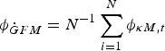 $\phi_{\dot {G}FM} =N^{-1}\sum_{i=1}^{N} {\phi_{\kappa M\comma t}}$
, where
 $\phi _{\kappa M\comma t} $
is the FMOLS estimator. And the associated t-statistic is given as
 $$t_{\dot{G}FM} =N^{-1/2}\sum_{t=1}^N t \phi_{\dot{\kappa}M\comma t}\comma \;$$
where
 $$t\hat{\phi}_{\dot{\kappa}M\comma t} = \lpar \hat{\phi}_{\dot{\kappa}M\comma i}- \phi_0\rpar \left(\hat{\Omega}_{11t}^{-1} \sum_{t=1}^T \lpar x_{it}-\bar{x}_{it}\rpar^2\right)^{1/2}.$$
5.3.2. DOLS estimators
The DOLS model is given as
 $y_{it}=\alpha_{i} +\beta_{i} x_{it} +\sum_{j=-q_{i}}^{qi} {\lambda_{iq} \Delta x_{it-q}} +u^{\ast}_{it}$
and the group-mean panel DOLS estimator is
 $\hat {\phi}_{B^{\ast} S} =\left[N^{-1}\sum_{i=1}^{N} \left({\sum_{t=1}^{T} {n_{it} {n}'_{it}}}\right)^{-1}\right.\break \left.\left({\sum_{t=1}^{T} {n_{it} \tilde {s}_{it}}} \right)\right]_{1}\comma \; $
where n
it
is the
 $2\lpar \hbox{K}+1\rpar \times 1$
vector of regressors
 $n_{it}=\lpar x_{it} -\hat {x}_{it} \comma \; \Delta x_{it-K}\comma \; \ldots\comma \; \Delta x_{it+K} \rpar $
.
 $\tilde {y}_{it} =y_{it} -\bar{y}_{it}$
. The associated t-statistic for the between-dimension estimator is given as
 $$t_{\phi Dj^\ast} =\lpar \phi_{D\comma i^\ast} -\phi_0 \rpar \left(\hat {\sigma}_t^{-2}\sum_{t=1}^T {\lpar x_{it} -\bar {x}_{it}\rpar^2}\right)^{1/2}.$$
5.4. Panel trivariate Granger causality test
Bivariate Granger causality models received many criticisms for being incomplete models that omitted important variables. This is because, when a third variable was included in the causality test, the bivariate models produce unreliable results (Caporale and Pittis, Reference Caporale and Pittis1997; Odhiambo, Reference Odhiambo2008). Some papers on the relation between economic growth, energy consumption and CO2 emissions used trivariate Granger causality models (see Odhiambo, Reference Odhiambo2009; Acaravci and Öztürk, 2010; Gao and Zhang, Reference Gao and Zhang2014).
The trivariate Granger causality model between variables based on the ECM was constructed as follows:
 $$\Delta y_{it} =\lambda_{1j} +\sum_{k=1}^m {\alpha_{\rm ik} \Delta y_{\rm it-k}} +\sum_{k=1}^m {\vartheta _{ik} X_{\rm it-k}} +\zeta_0 ECM_{\rm t-1} +\varepsilon_{\rm 1t} $$
 $$\Delta x_{it} =\lambda_{0} + \sum_{k=1}^{m} {\alpha_{\rm 2ik} \Delta x_{\rm it-k}} +\sum_{k=1}^m \vartheta_{\rm 2ik} \Delta y_{\rm it-k} +\zeta_1 ECM_{t-1} +\varepsilon_{\rm 2t}\comma \; $$
where residuals
 $\varepsilon_{t}$
are independently and normally distributed (i.i.d) with zero mean and constant variance, and ζ is a parameter indicating the speed of adjustment to the equilibrium level after a shock. Granger causality can be examined in short-run Granger causalities by
 $H_{0} \colon \vartheta_{ik} =0$
and
 $H_{1} \colon \vartheta_{ik} \ne 0$
in equation (1), and
 $H_{0} \colon \vartheta_{2ik} =0$
and
 $H_{1} \colon \vartheta_{2ik} \ne 0$
in equation (2) for all i. With regard to the long –run causality in equations (1) and (2), long-run Granger causalities are tested from the error-correction terms (ECTs) in those equations by
 $H_{0} \colon \zeta_{0} =0$
,
 $H_{0} \colon \zeta_{1} =0_{}$
for equations (1) and (2). And lastly, strong causality was tested. The strong causalities are tested by
 $H_{0} \colon \vartheta_{ik} =\zeta_{0} =0$
and
 $H_{0} \colon \vartheta _{2ik} =\zeta_{1} =0$
in equations (1) and (2).
6. Empirical results
In this paper, the econometric application was applied in four steps.
-
(i) Three panel unit root tests – LLC, IPS and CIPS – were used.
-
(ii) Cointegration was tested with the use of panel Johansen, Pedroni and PARDL tests.
-
(iii) The long-run coefficients were determined by PMG, FMOLS and DOLS methods.
-
(iv) Lastly, the causal relationship was determined with the panel trivariate Granger causality test.
6.1. The results of panel unit root tests
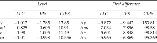
The results determined by panel unit root tests are reported in table 2. The parameters in the panel data variables are stationary in the first difference.
Panel unit root test

6.2. Panel cointegration results
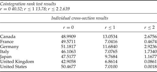
The Johansen cointegration results are given in table 3. While the H0 hypothesis was rejected for all countries, the H1 hypothesis was accepted.
Johansen cointegration results

The results of the Pedroni test are shown in table 4. Based on the results, the null hypothesis is rejected.
Pedroni cointegration test results

The Pedroni and Johansen tests accepted the existence of one cointegrating vector but they did not determine the coefficients of parameters.
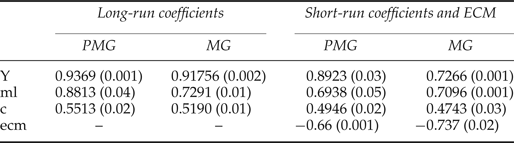
In this process, the PMG estimation and MG estimation are shown in table 5.
PMG and MG tests

Notes: The values in parentheses show P > |z|
The PMG and MG results indicated the existence of a strong relationship between CO2 emissions and militarization, between CO2 emissions and GDP, and between CO2 emissions and energy consumption. In the long run, the militarization elasticity of CO2 emissions was found to be 0.881 in PMG and 0.729 in MG. The income elasticity of CO2 emissions is determined as 0.936 (PMG) and 0.917 (MG) for the long run and as 0.892 (PMG) and 0.73 (MG) for the short run.
In comparing the PMG and MG estimators, it was determined that the estimated long-run elasticities are statistically significant as expected. However, the PMG estimate of the militarization, energy consumption and income elasticity is larger in magnitude than the coefficients estimated by the MG model.
The ECM coefficient indicated a mechanism to correct the disequilibrium between variables. The ECM coefficients are estimated as −0.66 and −0.737. They showed a rapid speed of adjustment of any disequilibrium towards long-run equilibrium.
6.3. FMOLS and DOLS results
Table 6 showed FMOLS and DOLS results. The coefficients determined from models are statistically significant at the 1 per cent significance level. The FMOLS and DOLS results exhibited similar results in magnitude and sign with each other and panel ARDL. The FMOLS results indicated that: a 1 per cent increase in m increases CO2 emissions by 0.913 per cent; a 1 per cent increase in y increases CO2 emissions by 0.923 per cent; and a 1 per cent increase in energy consumption increases CO2 emissions by 0.51 per cent. In the DOLS results, a 1 per cent increase in militarization increases CO2 emissions by 0.91 per cent, and CO2 emissions increase by 0.92 per cent if there is a 1 per cent increase in GDP.
FMOLS and DOLS results

The results obtained from panel ARDL, FMOLS and DOLS methods determined that the militarization, GDP and energy consumption have a significant positive impact on CO2 emissions. The results show that an increase in militarization, economic growth and energy consumption increase environmental pollution. Similarly to our findings, Givens (Reference Givens2014) found that militarization has a significant effect on environmental degradation, and Bildirici (Reference Bildirici2015) determined a statistically significant causal relation between defense expenditure and energy consumption.
6.4. Causality results
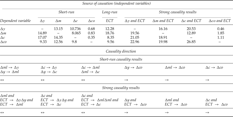
When the ECT is statistically significant, a change in one variable is expected to influence the other variable through a feedback system, signing a causal link among variables: co, y, ml and c (table 7).
Panel trivariate Granger causality test

In the long run, the coefficients of ECTs in all equations are significant. The result of the significance of the interactive term of energy consumption–ECT, militarization–ECT and economic growth–ECT in the emissions equation is in line with the causality which runs from energy consumption, economic growth and militarization to CO2 emissions. This finding reveals that whenever there is a shock to the system, energy consumption, militarization and economic growth would make a short[run adjustment to restore long[run equilibrium. Evidence was found of bidirectional causality between militarization and economic growth, between energy consumption and economic growth, between energy consumption and militarization, and between CO2 emissions and economic growth. Furthermore, there is unidirectional causality from militarization to CO2 emissions, from economic growth to CO2 emissions and from energy consumption to CO2 emissions. This supports the coefficients determined by the FMOLS, DOLS and panel ARDL models.
According to the results, the two-way causal relation between economic growth and militarization postulates that military expenditure plays a crucial role in economic growth and the reverse. Since an increase in militarization has a positive impact on economic growth, the policies that reduce militarization can negatively affect the economic growth. This result and results of a causal link between militarization and energy consumption, and between militarization and economic growth are similar to the findings of Bildirici (Reference Bildirici2015).
Bidirectional causality between energy consumption and economic growth supports the feedback hypothesis. The results of causality between energy consumption and CO2 emissions are consistent with the findings of Soytas et al. (Reference Soytas, Sari and Ewing2007) for the US, Zhang and Cheng (Reference Zhang and Cheng2009) for China, Pao and Tsai (Reference Pao and Tsai2011) for BRIC countries, Omri (Reference Omri2013) for 14 MENA countries, and Bildirici and Bakirtas (Reference Bildirici and Bakirtas2016) for BRICTS countries.
According to our results, militarization, economic growth and energy consumption have a positive significant impact on CO2 emissions per capita for all the countries. This indicates that an increase in militarization, economic growth and energy consumption raises the carbon emissions in G7 countries.
7. Conclusions and policy implications
In this paper, the relation between CO2 emissions, economic growth, energy consumption and militarization as the most ecologically destructive human production was analyzed by panel cointegration methods (Pedroni, Johansen, PARDL) and panel trivariate causality methods. The relationship between CO2 emissions, militarization, economic growth and energy consumption was positive and significant and there was a short-run as well as a long-run relationship.
The two-way causal relation between economic growth and militarization and between energy consumption and economic growth postulates that militarization and energy consumption play a crucial role in economic growth. The two-way causal relation between militarization and energy consumption, and between per capita GDP and energy consumption postulates that the energy conservation policies that reduce energy consumption negatively affect militarization and economic growth. The evidence of bidirectional causality between energy consumption and militarization determined that militarization increases energy consumption. Militarization and economic growth showed impacts on energy consumption. Unidirectional causality was found from militarization to CO2 emissions, from economic growth to CO2 emissions and from energy consumption to CO2 emissions. Militarization and energy consumption have an impact on CO2 emissions.
Our results determined that military establishments have very important impacts on energy consumption and that energy consumption and militarization play a crucial role in economic growth as crucial factors in improving the quality of life.
Causality results show a one-way causal link from militarization to CO2 emissions and from energy consumption to CO2 emissions, all without feedback. If G7 countries would like to reduce their emissions levels, they have to reduce not only energy consumption per unit of output but they also can sacrifice their militarization. A most important alternative option is to increase the use of renewable energy resources. Fighting against environmental pollution should be the most important policy.