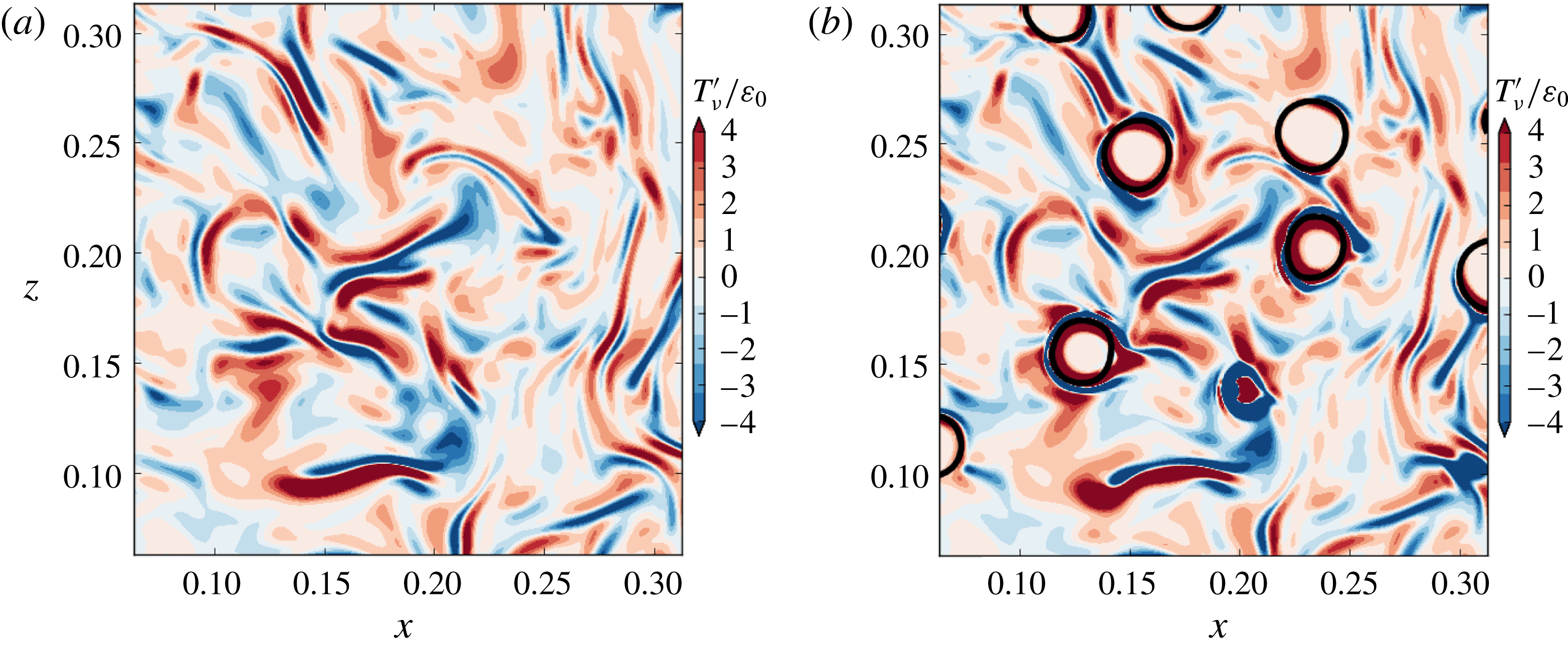
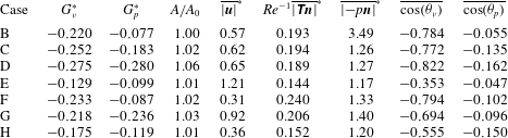
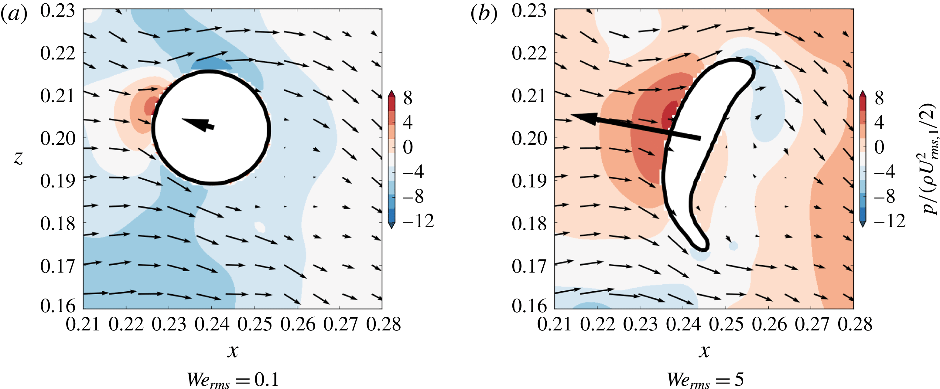
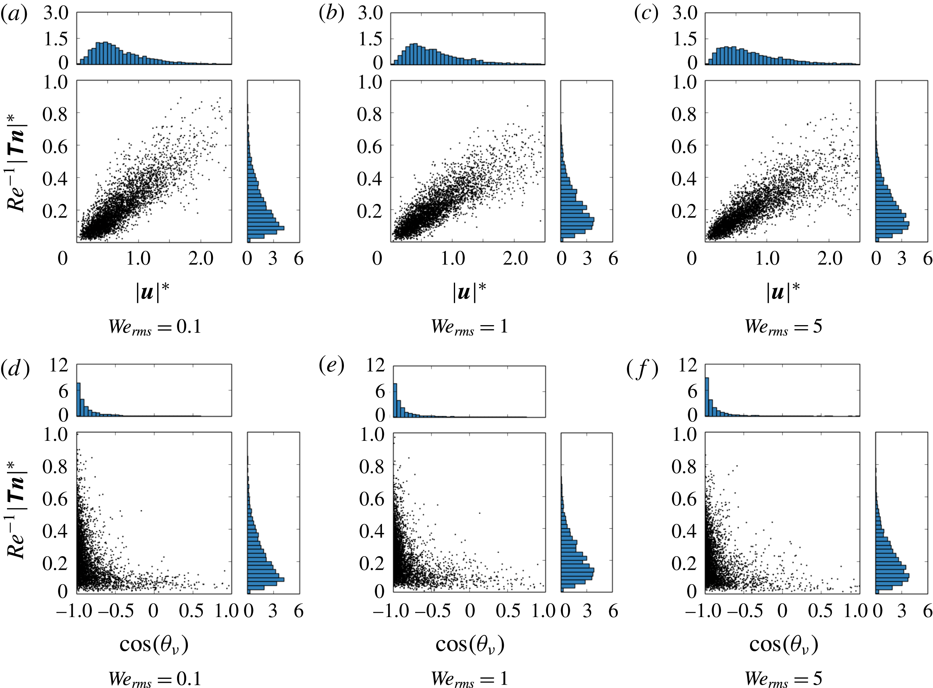
1 Introduction
The interaction of dispersed droplets and turbulence is important in many natural and industrial processes, e.g. rain formation (Shaw Reference Shaw2003), liquid–liquid emulsion (Berkman & Calabrese Reference Berkman and Calabrese1988), spray cooling (Qin et al. Reference Qin, Loth, Li, Simon and Van de Ven2014) and spray atomization in combustors (Sirignano Reference Sirignano1983; Faeth, Hsiang & Wu Reference Faeth, Hsiang and Wu1995). In these flows the droplet volume fraction is typically of the order of 1 %–10 % such that the turbulence is altered by droplet feedback on the surrounding fluid and by droplet–droplet interactions, placing the flow in the four-way coupling regime (Elghobashi Reference Elghobashi1994).
Direct numerical simulation (DNS) has proven to be an invaluable tool in understanding turbulence modulation in two-phase flows (Balachandar & Eaton Reference Balachandar and Eaton2010), because it resolves the full range of temporal and spatial scales present in the flow at the continuum level. Spherical particles (or droplets) in isotropic turbulence can be broadly classified by their diameter
 $D$
relative to the smallest turbulent length scale (the Kolmogorov scale,
 $\unicode[STIX]{x1D702}$
) as sub-Kolmogorov size (
 $D\ll \unicode[STIX]{x1D702}$
) or finite size (
 $D>\unicode[STIX]{x1D702}$
). For
 $D\ll \unicode[STIX]{x1D702}$
, the extent to which solid particles modulate isotropic turbulence, for fixed volume fraction and mass loading, is fully characterized by the Stokes number
 $St=\unicode[STIX]{x1D70F}_{p}/\unicode[STIX]{x1D70F}_{\unicode[STIX]{x1D702}}$
(Ferrante & Elghobashi Reference Ferrante and Elghobashi2003; Yang & Shy Reference Yang and Shy2005), where
 $\unicode[STIX]{x1D70F}_{p}$
is the particle response time and
 $\unicode[STIX]{x1D70F}_{\unicode[STIX]{x1D702}}$
is the Kolmogorov time scale. If
 $D>\unicode[STIX]{x1D702}$
,
 $St$
is no longer an appropriate indicator of turbulence modulation (Lucci, Ferrante & Elghobashi Reference Lucci, Ferrante and Elghobashi2011).
In the present paper, we consider finite-size droplets of Taylor length scale size (
 $D\approx \unicode[STIX]{x1D706}$
, where
 $\unicode[STIX]{x1D706}$
is the Taylor length scale) in homogeneous isotropic turbulence without phase change and gravity. Compared to finite-size particle–turbulence interaction (Lucci, Ferrante & Elghobashi Reference Lucci, Ferrante and Elghobashi2010), the interaction of finite-size droplets and turbulence is expected to incorporate new physical mechanisms. Compared to solid particles, droplets can deform, develop internal circulation and break up and coalesce with other droplets. The first two processes are characterized by two additional non-dimensional parameters: the Weber number,
 $\mathit{We}$
, and the viscosity ratio between the droplet fluid and carrier fluid
 $\unicode[STIX]{x1D707}_{d}/\unicode[STIX]{x1D707}_{c}$
. To the best of our knowledge, the effects of varying
 $\mathit{We}$
and
 $\unicode[STIX]{x1D707}_{d}/\unicode[STIX]{x1D707}_{c}$
have not been investigated in droplet-laden isotropic turbulence. Also, we have several fundamental questions for understanding and predicting droplet-laden turbulent flows: (i) what are the effects of surface tension, droplet deformation and droplet internal circulation? (ii) what are the effects of droplet–droplet interactions? and (iii) what are the underlying physical mechanisms? Answering these questions will aid in developing mathematical models, e.g. subgrid-scale (SGS) models for large eddy simulation, to simulate practical flows in complex geometries.
We perform a parametric study of DNS of droplet-laden isotropic turbulence in which we vary the Weber number based on the r.m.s. velocity of turbulence (
 $\mathit{We}_{rms}$
), density ratio (
 $\unicode[STIX]{x1D70C}_{d}/\unicode[STIX]{x1D70C}_{c}$
) and viscosity ratio (
 $\unicode[STIX]{x1D707}_{d}/\unicode[STIX]{x1D707}_{c}$
), as well as DNS of droplet-free isotropic turbulence to serve as a reference. The only accurate approach to perform DNS of particles or droplets in turbulence whose diameter
 $D>\unicode[STIX]{x1D702}$
is to numerically resolve the fluid motion around each individual moving body. Few studies which resolve the flow around freely moving particles in a turbulent flow have been published: Ten Cate et al. (Reference Ten Cate, Derksen, Portela and Van den Akker2004), Zhang & Prosperetti (Reference Zhang and Prosperetti2005), Lucci et al. (Reference Lucci, Ferrante and Elghobashi2010), Picano, Breugem & Brandt (Reference Picano, Breugem and Brandt2015). There are even fewer studies which fully resolve the flow around droplets, and most are limited to
 $\unicode[STIX]{x1D70C}_{d}/\unicode[STIX]{x1D70C}_{c}=1$
and
 $\unicode[STIX]{x1D707}_{d}/\unicode[STIX]{x1D707}_{c}=1$
(e.g. Perlekar et al.
Reference Perlekar, Biferale, Sbragaglia, Srivastava and Toschi2012; Baraldi, Dodd & Ferrante Reference Baraldi, Dodd and Ferrante2014). Dodd & Ferrante (Reference Dodd and Ferrante2014) reported the results of one simulation for
 $\mathit{We}_{rms}=1$
 $\unicode[STIX]{x1D70C}_{d}/\unicode[STIX]{x1D70C}_{c}=10$
and
 $\unicode[STIX]{x1D707}_{d}/\unicode[STIX]{x1D707}_{c}=1$
.
The limited number of DNS studies of finite-size droplets in turbulence is explained by the increased complexity of the algorithms and the high computational cost associated with resolving the flow field in the exterior and interior of freely moving droplets. Sirignano (Reference Sirignano1999) identified four main physical challenges in simulating droplet-laden turbulent flows; they are: (i) resolving the smallest turbulent eddies (Kolmogorov scale), (ii) resolving the velocity gradients in the interfacial transition region, (iii) resolving the flow between droplets and (iv) resolving the flow in the droplet interiors. In addition, we have identified three primary numerical challenges in simulating droplet-laden turbulent flows; they are (i) developing a mass-conserving algorithm to track or capture the droplet volumes in space and time, (ii) developing a temporal and spatial discretization that is accurate and stable for large density and viscosity ratios and (iii) accurately modelling the effects of surface tension. Except for resolving the thin (tens of nanometres) liquid film that develops during droplet coalescence and breakup, we have overcome the physical and numerical challenges by developing a mass-conserving volume-of-fluid (VoF) scheme (Baraldi et al. Reference Baraldi, Dodd and Ferrante2014) and a fast two-fluid pressure-correction method (Dodd & Ferrante Reference Dodd and Ferrante2014).
The paper is organized as follows: the mathematical description is presented (§ 2), which includes the governing equations (§ 2.1) and the numerical method (§ 2.2). Next, the results are presented and discussed (§ 3), starting with a description of the initial conditions and the droplet properties (§ 3.1). Next, we introduce the turbulence kinetic energy budget for droplet-laden flows (§ 3.2). Then, we compare the time evolution of TKE in droplet-free to that in droplet-laden turbulence (§ 3.3), and study the interaction of the carrier and droplet fluid by analysing the TKE evolution of each phase (§ 3.4). Finally, we summarize the findings of this work (§ 4).
2 Mathematical description
2.1 Governing equations
The non-dimensional governing equations for an incompressible flow of two immiscible fluids are
 $$\begin{eqnarray}\displaystyle & \unicode[STIX]{x1D735}\boldsymbol{\cdot }\boldsymbol{u}=0, & \displaystyle\end{eqnarray}$$
 $$\begin{eqnarray}\displaystyle & \displaystyle \frac{\unicode[STIX]{x2202}\boldsymbol{u}}{\unicode[STIX]{x2202}t}+\unicode[STIX]{x1D735}\boldsymbol{\cdot }(\boldsymbol{u}\boldsymbol{u})=\frac{1}{\unicode[STIX]{x1D70C}}\left[-\unicode[STIX]{x1D735}p+\frac{1}{\mathit{Re}}\unicode[STIX]{x1D735}\boldsymbol{\cdot }(2\unicode[STIX]{x1D707}\unicode[STIX]{x1D64E})+\frac{1}{\mathit{We}}\boldsymbol{f}_{\unicode[STIX]{x1D70E}}\right], & \displaystyle\end{eqnarray}$$
 $\boldsymbol{u}=\boldsymbol{u}(\boldsymbol{x},t)$
is the fluid velocity,
 $p=p(\boldsymbol{x},t)$
is the pressure,
 $\unicode[STIX]{x1D70C}=\unicode[STIX]{x1D70C}(\boldsymbol{x},t)$
is the density,
 $\unicode[STIX]{x1D707}=\unicode[STIX]{x1D707}(\boldsymbol{x},t)$
is the dynamic viscosity,
 $\unicode[STIX]{x1D64E}=\unicode[STIX]{x1D64E}(\boldsymbol{x},t)$
is the strain-rate tensor (
 $\unicode[STIX]{x1D64E}=[\unicode[STIX]{x1D735}\boldsymbol{u}+(\unicode[STIX]{x1D735}\boldsymbol{u})^{\text{T}}]/2$
).
 $\mathit{Re}$
and
 $\mathit{We}$
are the Reynolds and Weber numbers, respectively, which are defined as:
 $$\begin{eqnarray}\mathit{Re}=\frac{\tilde{U} \tilde{L}\tilde{\unicode[STIX]{x1D70C}}_{c}}{\tilde{\unicode[STIX]{x1D707}}_{c}},\quad \mathit{We}=\frac{\tilde{\unicode[STIX]{x1D70C}}_{c}\tilde{U} ^{2}\tilde{L}}{\tilde{\unicode[STIX]{x1D70E}}},\end{eqnarray}$$
where
 $\tilde{U}$
,
 $\tilde{L}$
,
 $\tilde{\unicode[STIX]{x1D70C}}_{c}$
,
 $\tilde{\unicode[STIX]{x1D707}}_{c}$
and
 $\tilde{\unicode[STIX]{x1D70E}}$
denote, in order, the reference dimensional velocity, length, carrier-fluid density, carrier-fluid dynamic viscosity and surface tension coefficient used to non-dimensionalize the governing equations (2.1a
) and (2.1b
). The subscripts
 $c$
and
 $d$
indicate the carrier fluid and droplet fluid, respectively. We have chosen to non-dimensionalize the density and dynamic viscosity in (2.1b
) by choosing the carrier fluid as the reference phase, such that
 $\unicode[STIX]{x1D70C}_{c}=1$
and
 $\unicode[STIX]{x1D707}_{c}=1$
.
 $\boldsymbol{f}_{\unicode[STIX]{x1D70E}}=\boldsymbol{f}_{\unicode[STIX]{x1D70E}}(\boldsymbol{x},t)$
is the force per unit volume due to surface tension,
 $$\begin{eqnarray}\boldsymbol{f}_{\unicode[STIX]{x1D70E}}=\unicode[STIX]{x1D705}\unicode[STIX]{x1D6FF}(s)\boldsymbol{n},\end{eqnarray}$$
where
 $\unicode[STIX]{x1D705}=\unicode[STIX]{x1D705}(\boldsymbol{x},t)$
is the curvature of the droplet interface,
 $\boldsymbol{n}=\boldsymbol{n}(\boldsymbol{x},t)$
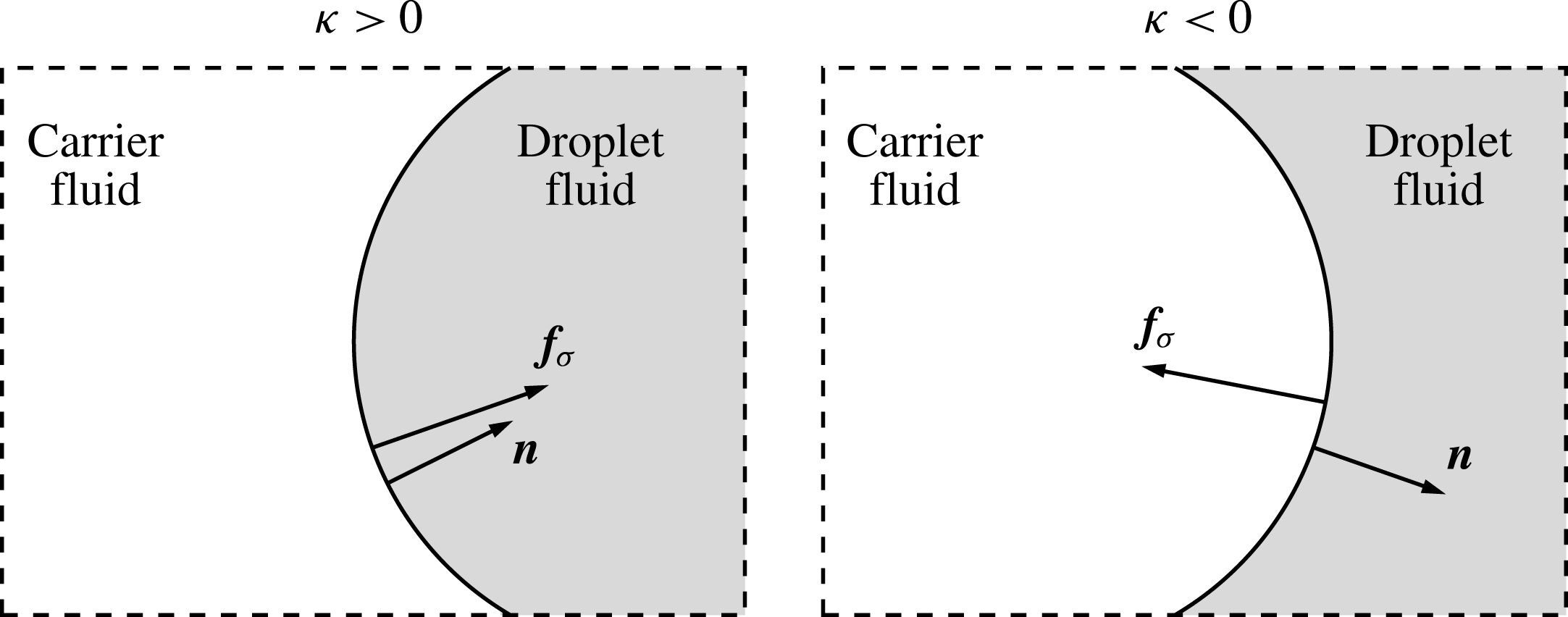
is the unit vector that is normal to the interface and directed towards the interior of the droplet,
 $\unicode[STIX]{x1D6FF}$
is the Dirac
 $\unicode[STIX]{x1D6FF}$
-function that is needed to impose
 $\boldsymbol{f}_{\unicode[STIX]{x1D70E}}$
only at the interface position and
 $s$
is a normal coordinate centred at the interface, such that
 $s=0$
at the interface. Figure 1 illustrates the direction of the interface normal
 $\boldsymbol{n}$
and the sign of the interface curvature
 $\unicode[STIX]{x1D705}$
. Throughout the paper, all quantities are dimensionless unless they are accented with
 ${\sim}$
. Also, we sometimes interchange the symbol
 $\mathit{Re}^{-1}$
with
 $\unicode[STIX]{x1D708}$
and
 $\mathit{We}^{-1}$
with
 $\unicode[STIX]{x1D70E}$
. The jump conditions for
 $\boldsymbol{u}$
are derived in § A.1 and those for
 $p$
and
 $2\unicode[STIX]{x1D707}\unicode[STIX]{x1D64E}$
in § A.2.
Schematic of the interface between two fluids which shows the surface tension force (
 $\boldsymbol{f}_{\unicode[STIX]{x1D70E}}$
), interface normal (
 $\boldsymbol{n}$
) and the sign convention of the curvature (
 $\unicode[STIX]{x1D705}$
).

2.2 Numerical method
In § 2.2.1 we describe the pressure-correction method that is used to solve numerically the two-fluid governing equations (2.1a ) and (2.1b ). This method is coupled to the VoF method (§ 2.2.2), which is used to capture the motion of the droplet interface.
2.2.1 Pressure-correction method
We solve the governing equations (2.1a
) and (2.1b
) throughout the whole computational domain, including the interior of the droplets. The domain is a periodic cube with side length
 $\mathscr{L}=1$
. The governing equations are discretized in space in an Eulerian framework using the second-order central difference scheme on a uniform staggered mesh.
The solution algorithm proceeds by advecting the volume fraction of the droplet fluid,
 $C(\boldsymbol{x},t)$
, based on the known velocity field
 $\boldsymbol{u}^{n}$
. The volume fraction has value
 $C=0$
in the carrier fluid,
 $C=1$
in the droplet fluid and
 $0<C<1$
in cells containing the droplet interface. After computing
 $C^{n+1}$
(§ 2.2.2), the density and viscosity can be computed at time level
 $n+1$
as
 $$\begin{eqnarray}\left.\begin{array}{@{}c@{}}\displaystyle \unicode[STIX]{x1D70C}^{n+1}(\boldsymbol{x})=\unicode[STIX]{x1D70C}_{d}C^{n+1}(\boldsymbol{x})+\unicode[STIX]{x1D70C}_{c}[1-C^{n+1}(\boldsymbol{x})]\\ \displaystyle \unicode[STIX]{x1D707}^{n+1}(\boldsymbol{x})=\unicode[STIX]{x1D707}_{d}C^{n+1}(\boldsymbol{x})+\unicode[STIX]{x1D707}_{c}[1-C^{n+1}(\boldsymbol{x})].\end{array}\right\}\end{eqnarray}$$
Next, an approximate velocity is computed by first defining
 $\boldsymbol{R}\boldsymbol{U}^{n}$
as
 $$\begin{eqnarray}\displaystyle \boldsymbol{R}\boldsymbol{U}^{n}=-\unicode[STIX]{x1D735}\boldsymbol{\cdot }(\boldsymbol{u}^{n}\boldsymbol{u}^{n})+\frac{1}{\mathit{Re}}\left[\frac{1}{\unicode[STIX]{x1D70C}^{n+1}}\unicode[STIX]{x1D735}\boldsymbol{\cdot }(2\unicode[STIX]{x1D707}^{n+1}\unicode[STIX]{x1D64E}^{n})\right]+\frac{1}{\mathit{We}}\left[\frac{\unicode[STIX]{x1D705}^{n+1}\unicode[STIX]{x1D735}C^{n+1}}{\bar{\unicode[STIX]{x1D70C}}}\right]. & & \displaystyle\end{eqnarray}$$
The surface tension force,
 $\boldsymbol{f}_{\unicode[STIX]{x1D70E}}$
, is computed by using Brackbill’s continuum surface force (CSF) approach (Brackbill, Kothe & Zemach Reference Brackbill, Kothe and Zemach1992):
 $$\begin{eqnarray}\boldsymbol{f}_{\unicode[STIX]{x1D70E}}=\frac{\unicode[STIX]{x1D70C}}{\bar{\unicode[STIX]{x1D70C}}}\unicode[STIX]{x1D705}\unicode[STIX]{x1D735}C,\end{eqnarray}$$
where
 $\bar{\unicode[STIX]{x1D70C}}\equiv (\unicode[STIX]{x1D70C}_{1}+\unicode[STIX]{x1D70C}_{2})/2$
. The interface curvature
 $\unicode[STIX]{x1D705}^{n+1}$
is computed using the height-function method (Cummins, Francois & Kothe Reference Cummins, Francois and Kothe2005) with improvements developed by López et al. (Reference López, Zanzi, Gómez, Zamora, Faura and Hernández2009).
The equations are integrated in time using the second-order Adams–Bashforth scheme:
 $$\begin{eqnarray}\frac{\boldsymbol{u}^{\ast }-\boldsymbol{u}^{n}}{\unicode[STIX]{x0394}t}=\frac{3}{2}\boldsymbol{R}\boldsymbol{U}^{n}-\frac{1}{2}\boldsymbol{R}\boldsymbol{U}^{n-1}.\end{eqnarray}$$
The pressure is computed by solving the Poisson equation (Dodd & Ferrante Reference Dodd and Ferrante2014):
 $$\begin{eqnarray}\unicode[STIX]{x1D6FB}^{2}p^{n+1}=\unicode[STIX]{x1D735}\boldsymbol{\cdot }\left[\left(1-\frac{\unicode[STIX]{x1D70C}_{0}}{\unicode[STIX]{x1D70C}^{n+1}}\right)\unicode[STIX]{x1D735}p^{\ast }\right]+\frac{\unicode[STIX]{x1D70C}_{0}}{\unicode[STIX]{x0394}t}\unicode[STIX]{x1D735}\boldsymbol{\cdot }\boldsymbol{u}^{\ast },\end{eqnarray}$$
where we have split the pressure gradient term (Dong & Shen Reference Dong and Shen2012) as
 $$\begin{eqnarray}\frac{1}{\unicode[STIX]{x1D70C}^{n+1}}\unicode[STIX]{x1D735}p^{n+1}\rightarrow \frac{1}{\unicode[STIX]{x1D70C}_{0}}\unicode[STIX]{x1D735}p^{n+1}+\left(\frac{1}{\unicode[STIX]{x1D70C}^{n+1}}-\frac{1}{\unicode[STIX]{x1D70C}_{0}}\right)\unicode[STIX]{x1D735}p^{\ast },\end{eqnarray}$$
where
 $\unicode[STIX]{x1D70C}_{0}=\text{min}(\unicode[STIX]{x1D70C}_{1},\unicode[STIX]{x1D70C}_{2})$
and
 $p^{\ast }=2p^{n}-p^{n-1}$
. The advantage of using (2.9) is that it yields a constant coefficient Poisson equation (2.8) which can be solved efficiently using direct methods. Equation (2.8) is solved directly using a combination of a two-dimensional fast Fourier transforms (FFT) in the
 $x$
–
 $y$
plane and Gauss elimination in the
 $z$
-direction (Schmidt, Schumann & Volkert Reference Schmidt, Schumann and Volkert1984). Finally, we update the velocity field by applying the pressure correction to
 $\boldsymbol{u}^{\ast }$
as
 $$\begin{eqnarray}\boldsymbol{u}^{n+1}=\boldsymbol{u}^{\ast }-\unicode[STIX]{x0394}t\left[\frac{1}{\unicode[STIX]{x1D70C}_{0}}\unicode[STIX]{x1D735}p^{n+1}+\left(\frac{1}{\unicode[STIX]{x1D70C}^{n+1}}-\frac{1}{\unicode[STIX]{x1D70C}_{0}}\right)\unicode[STIX]{x1D735}p^{\ast }\right].\end{eqnarray}$$
For solving the two-fluid Navier–Stokes equations, equations (2.1a
) and (2.1b
), the FFT-based method outlined above is 10–40 times faster than the standard multigrid-based pressure-correction method (Dodd & Ferrante Reference Dodd and Ferrante2014). An additional advantage is that, because (2.8) is solved directly,
 $\boldsymbol{u}^{n+1}$
is divergence-free to machine precision. Dodd & Ferrante (Reference Dodd and Ferrante2014) provides a complete description of the two-fluid pressure-correction method that includes verification and validation cases as well convergence tests demonstrating second-order accuracy in space and time for velocity and in space for pressure.
2.2.2 Volume-of-fluid (VoF) method
In the VoF method, the sharp interface between the two immiscible fluids is determined using the VoF colour function,
 $C$
, which represents the volume fraction of the droplet fluid in each computational cell. In our VoF method, the interface between the two fluids is reconstructed using a piecewise linear interface calculation (PLIC) (Youngs Reference Youngs1982). The interface reconstruction in each computational cell consists of two steps: the computation of the interface normal
 $\boldsymbol{n}=(n_{x},n_{y},n_{z})$
and the computation of the interface location. The algorithm that we use to evaluate the interface normal is a combination of the centred-columns method (Miller & Colella Reference Miller and Colella2002) and Youngs’ method (Youngs Reference Youngs1982) known as the mixed-Youngs-centred (MYC) method (Aulisa et al.
Reference Aulisa, Manservisi, Scardovelli and Zaleski2007).
If we consider a characteristic function
 $\unicode[STIX]{x1D712}$
that has value
 $\unicode[STIX]{x1D712}=1$
in the droplet fluid and
 $\unicode[STIX]{x1D712}=0$
in the carrier fluid,
 $\unicode[STIX]{x1D712}$
is governed by the following advection equation:
 $$\begin{eqnarray}\frac{\unicode[STIX]{x2202}\unicode[STIX]{x1D712}}{\unicode[STIX]{x2202}t}+\boldsymbol{u}\boldsymbol{\cdot }\unicode[STIX]{x1D735}\unicode[STIX]{x1D712}=0.\end{eqnarray}$$
The volume fraction
 $C_{i,j,k}$
of grid cell
 $i,j,k$
is related to the characteristic function
 $\unicode[STIX]{x1D712}$
by the integral relation
 $$\begin{eqnarray}C_{i,j,k}(t)=\frac{1}{V_{0}}\iiint _{V_{0}}\unicode[STIX]{x1D712}(\boldsymbol{x},t)\,\text{d}\boldsymbol{x},\end{eqnarray}$$
where
 $V_{0}$
is the volume of the
 $i,j,k$
cell.
The volume fraction
 $C$
is advanced in time using the Eulerian implicit–Eulerian algebraic–Lagrangian explicit (EI–EA–LE) algorithm originally proposed by Scardovelli et al. (Reference Scardovelli, Aulisa, Manservisi and Marra2002). The original EI–EA–LE algorithm is globally mass conserving but generates wisps and does not conserve the mass of the individual volumes captured in the flow. We have improved this method by adding redistribution and wisp-suppression algorithms (Baraldi et al.
Reference Baraldi, Dodd and Ferrante2014). The redistribution algorithm corrects small inconsistencies in the volume fraction values (i.e.
 $C<0$
and
 $C>1$
) that arise in the Eulerian algebraic (EA) step. The wisp-suppression algorithm removes small errors arising from the finite machine precision. Because our method is consistent and wisps-free, it conserves mass both globally and locally within each fluid in the absence of breakup and coalescence. Even with breakup and coalescence, in all the cases that will be presented, the total mass (and volume) of the droplets deviates less than 0.0002 % from the initial value.
Using the improved EI–EA–LE algorithm, the cell-centred volume fraction
 $C$
is advected using the face-centred velocity field
 $\boldsymbol{u}$
. The method displays second-order spatial accuracy for values of Courant–Friedrichs–Lewy (CFL) number
 ${\leqslant}0.1$
. Furthermore, the average geometrical error (
 $E_{g}=|C(\boldsymbol{x})-C_{\mathit{exact}}(\boldsymbol{x})|$
) is less than 1 % for a moving droplet with 30 grid cells or more across the diameter. The complete description of the method and the results are reported by Baraldi et al. (Reference Baraldi, Dodd and Ferrante2014).
Breakup and coalescence of fluid volumes is handled implicitly by the VoF method. For example, if two interfaces occupy the same computational cell during the VoF update from time level
 $n$
to
 $n+1$
, then the two VoF volumes are merged (or coalesced) automatically. This process is commonly referred to as numerical coalescence. Likewise, when the thickness of a droplet ligament becomes less than the grid spacing
 $h$
, it will break. Because the thickness of the film between drops can be several orders of magnitude smaller than the smallest length scales of the surrounding flow, fully resolving the film is prohibitively expensive from a computational standpoint. An alternative approach is to use a subgrid-scale model to determine whether the droplets will breakup or coalesce; however, such approaches are strongly dependent on the underlying film drainage model employed (Kwakkel, Breugem & Boersma Reference Kwakkel, Breugem and Boersma2013), and thus their predictive capabilities are uncertain. In the present simulations we do not use a subgrid-scale model and allow the droplets to numerically coalesce or breakup.
3 Results and discussion
3.1 Initial conditions and droplet properties
3.1.1 Carrier flow parameters and initial conditions
The initial velocity field was generated by prescribing the TKE spectrum
 $E(\unicode[STIX]{x1D705})$
and ensuring that the initial random velocity field is isotropic, divergence-free with respect to the discretized form of the continuity equation and that the velocity cross-correlation spectra,
 $R_{ij}(\unicode[STIX]{x1D705})$
, satisfy the realizability constraint (Schumann Reference Schumann1977).
The initial energy spectrum at time
 $t=0$
was prescribed as (Pope Reference Pope2000, § 6.5.3):
 $$\begin{eqnarray}E(\unicode[STIX]{x1D705})=1.5[\unicode[STIX]{x1D700}_{0}^{2/3}\unicode[STIX]{x1D705}^{-5/3}f_{L}(\unicode[STIX]{x1D705}L)f_{\unicode[STIX]{x1D702}}(\unicode[STIX]{x1D705}\unicode[STIX]{x1D702})],\end{eqnarray}$$
where
 $\unicode[STIX]{x1D705}$
is the wavenumber,
 $\unicode[STIX]{x1D700}_{0}$
is the initial dissipation rate of TKE,
 $L\equiv k_{0}^{3/2}/\unicode[STIX]{x1D700}_{0}$
, where
 $k_{0}$
is the initial TKE,
 $f_{L}$
is given by
 $$\begin{eqnarray}f_{L}(\unicode[STIX]{x1D705}L)=\left(\frac{\unicode[STIX]{x1D705}L}{[(\unicode[STIX]{x1D705}L)^{2}+c_{L}]^{1/2}}\right)^{11/3}\end{eqnarray}$$
and
 $f_{\unicode[STIX]{x1D702}}$
is given by
 $$\begin{eqnarray}f_{\unicode[STIX]{x1D702}}(\unicode[STIX]{x1D705}\unicode[STIX]{x1D702})=\exp \{-5.2\{[(\unicode[STIX]{x1D705}\unicode[STIX]{x1D702})^{4}+c_{\unicode[STIX]{x1D702}}^{4}]^{1/4}-c_{\unicode[STIX]{x1D702}}\}\},\end{eqnarray}$$
where
 $c_{L}=4.698$
and
 $c_{\unicode[STIX]{x1D702}}=0.416$
. The constants
 $c_{L}$
and
 $c_{\unicode[STIX]{x1D702}}$
are calculated such that
 $E(\unicode[STIX]{x1D705})$
and
 $2\mathit{Re}^{-1}\unicode[STIX]{x1D705}^{2}E(\unicode[STIX]{x1D705})$
integrate to
 $k_{0}$
and
 $\unicode[STIX]{x1D700}_{0}$
, respectively. The values of the dimensionless parameters at
 $t=0$
were
 $k_{0}=3.893\times 10^{-3}$
,
 $\unicode[STIX]{x1D700}_{0}=1.156\times 10^{-3}$
and
 $\mathit{Re}=6.42\times 10^{4}$
. These parameters yield an initial Reynolds number based on the Taylor length scale of
 $\mathit{Re}_{\unicode[STIX]{x1D706}0}=75$
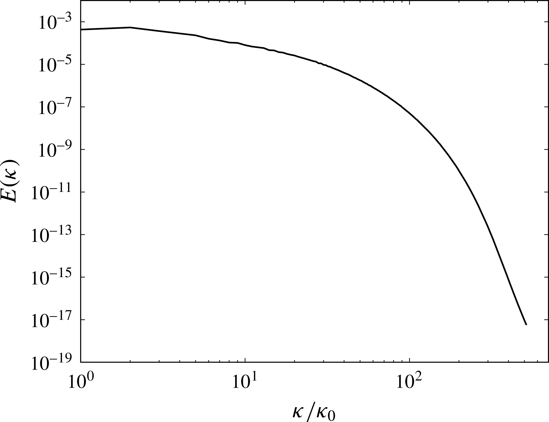
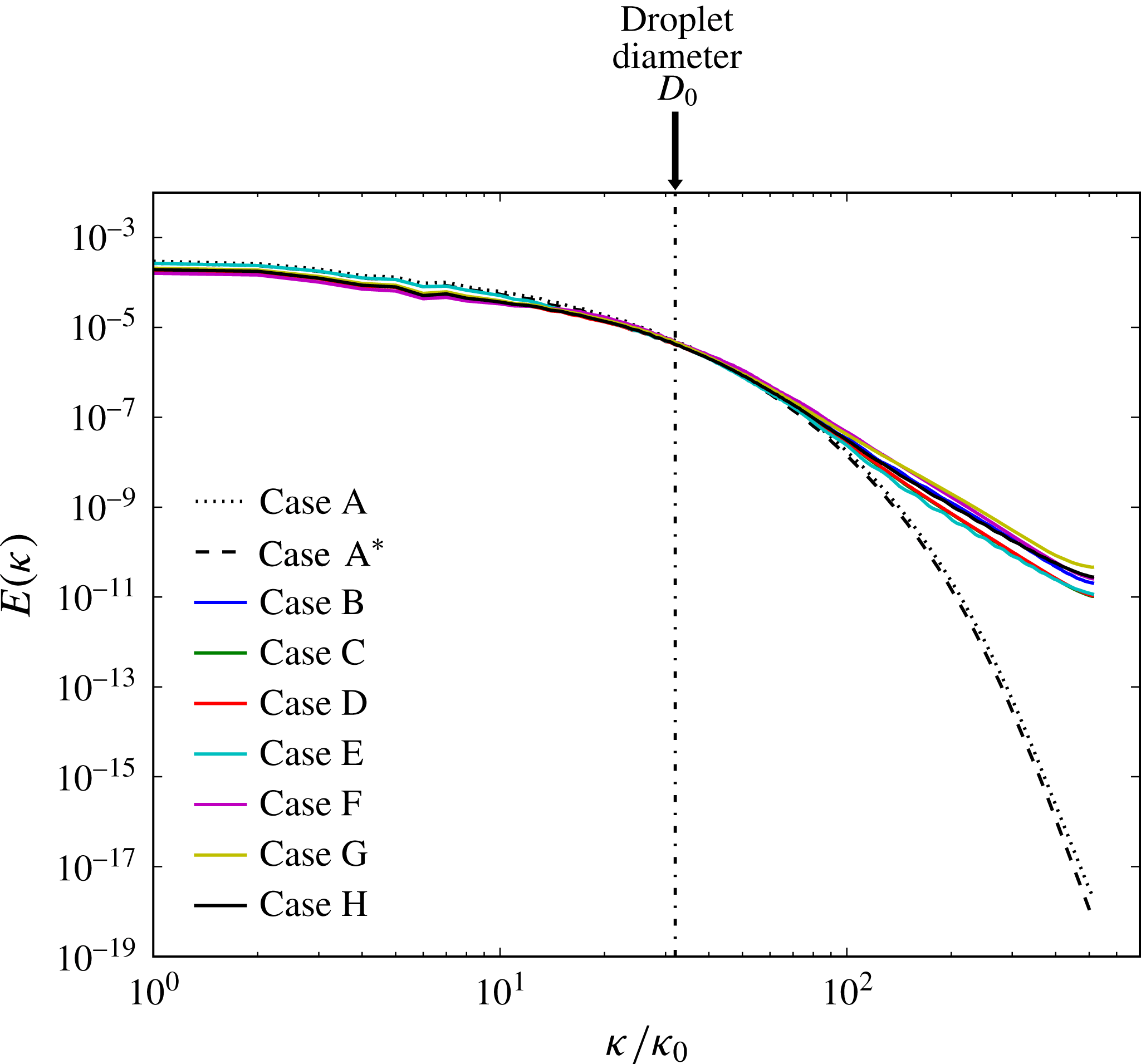
. Figure 2 shows the turbulence kinetic energy spectrum at
 $t=1$
in case A.
Turbulence kinetic energy spectrum at droplet release time,
 $t=1$
, in case A. The wavenumbers are normalized by the lowest non-zero wavenumber,
 $\unicode[STIX]{x1D705}_{0}=2\unicode[STIX]{x03C0}/\mathscr{L}$
.

Table 1 shows the dimensionless flow parameters at different times
 $t$
for the droplet-free flow (case A):
 $\ell$
and
 $\unicode[STIX]{x1D70F}_{\ell }$
are the integral length and time scales;
 $Re_{\ell }$
is the Reynolds number based on
 $\ell$
;
 $\unicode[STIX]{x1D706}$
is the Taylor length scale;
 $\unicode[STIX]{x1D702}$
and
 $\unicode[STIX]{x1D70F}_{\unicode[STIX]{x1D702}}$
are the Kolmogorov length and time scales. The values of the reference length and velocity scales used in normalizing the above quantities were
 $\tilde{L}_{ref}=0.032~\text{m}$
and
 $\tilde{U} _{ref}=26.7~\text{m}~\text{s}^{-1}$
, which together with the Reynolds number
 $\mathit{Re}$
, produce the appropriate value of the dimensional kinematic viscosity of the fluid (air at STP)
 $\tilde{\unicode[STIX]{x1D708}}_{ref}=1.33\times 10^{-5}~\text{m}^{2}~\text{s}^{-1}$
. The smallest scales of turbulence are well resolved as indicated by
 $\unicode[STIX]{x1D702}\unicode[STIX]{x1D705}_{\mathit{max}}\geqslant 1$
at all times, where
 $\unicode[STIX]{x1D705}_{\mathit{max}}=\unicode[STIX]{x03C0}N$
is the maximum resolved wavenumber and
 $N=1024$
is the number of grid points in each direction of our computational grid.
Flow parameters (dimensionless) at initial time (
 $t=0$
), droplet release time (
 $t=1$
) and at time
 $t=6$
in case A.

3.1.2 Droplet properties
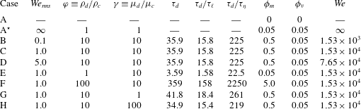
We perform one simulation (case A) of droplet-free flow and eight simulations (A
 $^{\star }$
–H) of droplet-laden isotropic turbulence (table 2). Case A
 $^{\star }$
is a limiting case in which the viscosity and density ratio are unity and the Weber number of the ‘droplets’ is infinity (i.e. the surface tension is null via (2.1b
)). We analyse the effects of varying the initial droplet Weber number (
 $We_{rms}=D_{0}U_{rms}^{2}\unicode[STIX]{x1D70C}_{c}/\unicode[STIX]{x1D70E}$
), droplet- to carrier-fluid density ratio (
 $\unicode[STIX]{x1D711}=\unicode[STIX]{x1D70C}_{d}/\unicode[STIX]{x1D70C}_{c}$
) and droplet- to carrier-fluid viscosity ratio (
 $\unicode[STIX]{x1D6FE}=\unicode[STIX]{x1D707}_{d}/\unicode[STIX]{x1D707}_{c}$
) in the three sets BCD, CEF, and CGH, respectively, while keeping the other two parameters constant. In cases B–D,
 $\mathit{We}_{rms}$
increases from 0.1 to 5.0 by decreasing the non-dimensional surface tension coefficient,
 $\unicode[STIX]{x1D70E}=1/\mathit{We}$
, in (2.3). In cases E, C and F,
 $\unicode[STIX]{x1D711}$
increases from 1 to 100 by increasing
 $\unicode[STIX]{x1D70C}_{d}$
. This in turn increases the mass loading ratio,
 $\unicode[STIX]{x1D719}_{m}$
, from 0.05 to 5.0. In cases G, C and H,
 $\unicode[STIX]{x1D6FE}$
increases from 1 to 100 by increasing
 $\unicode[STIX]{x1D707}_{d}$
. The droplet properties were selected for their engineering relevance in spray combustion devices. For all cases, the droplet volume fraction is
 $\unicode[STIX]{x1D719}_{v}=0.05$
, the initial number of droplets is
 $N_{d}=3130$
, and the initial droplet diameter is
 $D_{0}=0.03125$
(
 $\tilde{D}_{0}=1.0~\text{mm}$
), which is
 $20\unicode[STIX]{x1D702}_{1}$
(or
 $1.1\unicode[STIX]{x1D706}_{1}$
), where
 $\unicode[STIX]{x1D702}_{1}$
and
 $\unicode[STIX]{x1D706}_{1}$
are the Kolmogorov and Taylor length scales, respectively, at the time the droplets are released in the flow (
 $t=1$
). In table 2 we report the droplet response time, which for the Hadamard–Rybczyński solution (Hadamard Reference Hadamard1911; Rybczyński Reference Rybczyński1911) of creeping flow over a fluid sphere is
 $$\begin{eqnarray}\unicode[STIX]{x1D70F}_{d}=\frac{\unicode[STIX]{x1D70C}_{d}}{\unicode[STIX]{x1D70C}_{c}}\frac{D^{2}}{6\unicode[STIX]{x1D708}}\left(\frac{1+\unicode[STIX]{x1D6FE}}{2+3\unicode[STIX]{x1D6FE}}\right).\end{eqnarray}$$
Droplet properties (dimensionless) at release time (
 $t=1$
).

The prescribed initial velocity field
 $\boldsymbol{u}_{0}$
(see § 3.1) evolves free of droplets until
 $t=1$
, at which time
 $\mathit{Re}_{\unicode[STIX]{x1D706}1}=83$
and the skewness of the velocity derivative
 $S_{u}$
has reached the value
 $-0.50$
, indicating an established nonlinear transfer of TKE across the spectrum. At that time (
 $t=1$
), the droplets are randomly seeded at rest in the computational domain under the constraint that the distance between their centres must be at least
 $2.1D_{0}$
, such as to delay droplet–droplet coalescence in cases in which droplets coalesce. In all droplet-laden cases A
 $^{\star }$
–H, the initial positions of the droplets are identical. We also tested different initial random seedings of droplets, and found that the terms in the TKE budget varied by less than 1 % from the mean, except
 $\unicode[STIX]{x1D6F9}_{\unicode[STIX]{x1D70E}}$
. The power of the surface tension (
 $\unicode[STIX]{x1D6F9}_{\unicode[STIX]{x1D70E}}$
) is nearly independent of the droplet seeding for short times. After the onset of coalescence there is slight variation in the power of the surface tension – however, the overall trend is unchanged. Thus, we conclude that the results are essentially statistically independent of the initial positions of the droplets.
The droplets are resolved by 32 grid points per diameter (
 $D_{0}/\unicode[STIX]{x0394}x=32$
). This resolution provides a good compromise between VoF geometrical accuracy and computational efficiency, as shown in Baraldi et al. (Reference Baraldi, Dodd and Ferrante2014). The time step used is
 $\unicode[STIX]{x0394}t=0.1\unicode[STIX]{x0394}x$
and the simulations were stopped after 61 440 time steps at
 $t=6$
. At this time
 $\mathit{Re}_{\unicode[STIX]{x1D706}}=54$
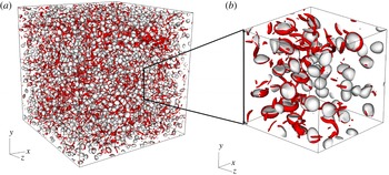
in case A. A snapshot of the computational domain is shown in figure 3, which depicts the droplets and vortical structures in case D at
 $t=1.5$
.
Instantaneous droplet interfaces in white (
 $C=0.5$
isosurface) and vortical structures in red (
 $\unicode[STIX]{x1D706}_{2}=-50$
isosurfaces, see Jeong & Hussain (Reference Jeong and Hussain1995) for definition of
 $\unicode[STIX]{x1D706}_{2}$
) in case D at
 $t=1.5$
. (a) Full domain (
 $1\times 1\times 1$
); (b) subdomain (
 $0.25\times 0.25\times 0.25$
).

When performing two-fluid flow simulations with surface tension and sharp-interface capturing like VoF, the small errors in the numerical calculation of the interface curvature,
 $\unicode[STIX]{x1D705}$
, generate spurious currents, i.e. unphysical velocity fluctuations near the interface. For droplets at rest or in uniform translation, the magnitude of the spurious currents increases with increasing Laplace number (Popinet Reference Popinet2009; Baraldi et al.
Reference Baraldi, Dodd and Ferrante2014),
 $$\begin{eqnarray}La=\frac{\unicode[STIX]{x1D70E}\unicode[STIX]{x1D70C}D}{\unicode[STIX]{x1D707}^{2}};\end{eqnarray}$$
therefore, we used the Laplace number to estimate their magnitude in the flow under study. In Baraldi et al. (Reference Baraldi, Dodd and Ferrante2014), we showed that, for a droplet in uniform translation and Laplace number of 100 000, the r.m.s. velocity of the spurious currents was less than 0.5 % of the translation speed. In cases B–H, the maximum Laplace number is 84 310, and therefore, we expect the magnitude of the spurious currents to be less than 0.5 % of
 $U_{rms}$
. To check if the simulations are tainted by spurious currents, we computed the specific energy spectrum,
 $E(\unicode[STIX]{x1D705})$
, by using the entire domain of the velocity field, in cases A–H at
 $t=3.5$
(figure 4). Spurious currents generate eddies with size of the order of the droplet diameter (see figure 17 of Baraldi et al.
Reference Baraldi, Dodd and Ferrante2014). Therefore, evidence of such currents would be marked by a source of energy at wavenumbers near the droplet diameter. Figure 4 shows that, in the droplet-laden cases (B–H), there is no unphysical bump in the spectra at wavenumbers associated with the droplet diameter. Thus, this shows that any kinetic energy added to the flow artificially by spurious currents is negligible.
Spectra of the specific turbulence kinetic energy at
 $t=3.5$
in cases A–H. The wavenumbers are normalized by the lowest non-zero wavenumber,
 $\unicode[STIX]{x1D705}_{0}=2\unicode[STIX]{x03C0}/\mathscr{L}$
.

Compared to the single-phase spectra (A and A
 $^{\ast }$
), the droplet-laden spectra (B–H) show increased energy at high wavenumbers. The increase in energy at high wavenumbers has been explained for finite-size solid particles in decaying isotropic turbulence. Lucci et al. (Reference Lucci, Ferrante and Elghobashi2010) showed that the presence of solid particles with
 $D\sim \unicode[STIX]{x1D706}$
broke the ‘order’ of large eddies and creates new eddies of size
 $D/2\sim \unicode[STIX]{x1D706}/2$
on the downstream side of the particle, thus increasing the energy at high wavenumbers. We believe that the presence of the droplet interface also breaks up large eddies, increasing the transfer rate of energy from low to high wavenumbers. Also, notice that
 $E(\unicode[STIX]{x1D705})$
was computed by using the entire domain, therefore the droplet-laden spectra in figure 4 includes specific energy from the droplet interiors. Still, the spectra are mostly comprised of the carrier-fluid specific energy (95 % by volume). To fully isolate the effects of droplets on the carrier flow would require limiting the FFT analysis to the carrier fluid.
3.2 Turbulence kinetic energy equations
In order to understand and explain the physical mechanisms of droplet and turbulence interactions, we use the evolution equations for the TKE of the two-fluid flow,
 $k(t)$
, the carrier-fluid flow,
 $k_{c}(t)$
, and the droplet-fluid flow,
 $k_{d}(t)$
. These equations are derived in appendix B.
The evolution equation for
 $k(t)$
is
 $$\begin{eqnarray}\frac{\text{d}k(t)}{\text{d}t}=-\unicode[STIX]{x1D700}(t)+\unicode[STIX]{x1D6F9}_{\unicode[STIX]{x1D70E}}(t),\end{eqnarray}$$
where
 $$\begin{eqnarray}k(t)\equiv \frac{1}{2}\langle \unicode[STIX]{x1D70C}u_{j}u_{j}\rangle ,\quad \unicode[STIX]{x1D700}(t)\equiv \frac{1}{\mathit{Re}}\langle \unicode[STIX]{x1D61B}_{ij}\unicode[STIX]{x1D61A}_{ij}\rangle ,\quad \unicode[STIX]{x1D6F9}_{\unicode[STIX]{x1D70E}}(t)\equiv \frac{1}{\mathit{We}}\langle u_{j}\,f_{\unicode[STIX]{x1D70E},j}\rangle ,\end{eqnarray}$$
where
 $\langle \cdots \rangle$
denotes spatial averaging over the entire domain.
 $\unicode[STIX]{x1D61B}_{ij}$
is the viscous stress tensor (
 $\unicode[STIX]{x1D61B}_{ij}=2\unicode[STIX]{x1D707}\unicode[STIX]{x1D61A}_{ij}$
) and
 $\unicode[STIX]{x1D61A}_{ij}$
is the strain-rate tensor, which was defined in § 2.1. In (3.7a–c
),
 $\unicode[STIX]{x1D700}(t)$
is the dissipation rate of TKE of the two-fluid flow and
 $\unicode[STIX]{x1D6F9}_{\unicode[STIX]{x1D70E}}(t)$
is the power of the surface tension, respectively. By definition,
 $\unicode[STIX]{x1D700}(t)$
is positive, thus it is a sink of TKE, whereas
 $\unicode[STIX]{x1D6F9}_{\unicode[STIX]{x1D70E}}(t)$
is either positive or negative, and thus a source or sink of TKE.
The evolution equation for
 $k_{c}(t)$
is
 $$\begin{eqnarray}\frac{\text{d}k_{c}(t)}{\text{d}t}=-\unicode[STIX]{x1D700}_{c}(t)+T_{\unicode[STIX]{x1D708},c}(t)+T_{p,c}(t),\end{eqnarray}$$
and the evolution equation for
 $k_{d}(t)$
is
 $$\begin{eqnarray}\frac{\text{d}k_{d}(t)}{\text{d}t}=-\unicode[STIX]{x1D700}_{d}(t)+T_{\unicode[STIX]{x1D708},d}(t)+T_{p,d}(t).\end{eqnarray}$$
The terms in (3.8) and (3.9) are defined as
 $$\begin{eqnarray}\left.\begin{array}{@{}c@{}}\displaystyle k_{c}(t)\equiv \frac{1}{2}\langle \unicode[STIX]{x1D70C}u_{j}u_{j}\rangle _{c},\quad \unicode[STIX]{x1D700}_{c}(t)\equiv \frac{1}{\mathit{Re}}\langle \unicode[STIX]{x1D61B}_{ij}\unicode[STIX]{x1D61A}_{ij}\rangle _{c},\\ \displaystyle T_{\unicode[STIX]{x1D708},c}(t)\equiv \frac{1}{\mathit{Re}}\frac{\unicode[STIX]{x2202}\langle \unicode[STIX]{x1D61B}_{ij}u_{j}\rangle _{c}}{\unicode[STIX]{x2202}x_{i}},\quad T_{p,c}(t)\equiv -\frac{\unicode[STIX]{x2202}\langle u_{j}p\rangle _{c}}{\unicode[STIX]{x2202}x_{j}},\end{array}\right\}\end{eqnarray}$$
and
 $$\begin{eqnarray}\left.\begin{array}{@{}c@{}}\displaystyle k_{d}(t)\equiv \frac{1}{2}\langle \unicode[STIX]{x1D70C}u_{j}u_{j}\rangle _{d},\quad \unicode[STIX]{x1D700}_{d}(t)\equiv \frac{1}{\mathit{Re}}\langle \unicode[STIX]{x1D61B}_{ij}\unicode[STIX]{x1D61A}_{ij}\rangle _{d},\\ \displaystyle T_{\unicode[STIX]{x1D708},d}(t)\equiv \frac{1}{\mathit{Re}}\frac{\unicode[STIX]{x2202}\langle \unicode[STIX]{x1D61B}_{ij}u_{j}\rangle _{d}}{\unicode[STIX]{x2202}x_{i}},\quad T_{p,d}(t)\equiv -\frac{\unicode[STIX]{x2202}\langle u_{j}p\rangle _{d}}{\unicode[STIX]{x2202}x_{j}},\end{array}\right\}\end{eqnarray}$$
where
 $\langle \ldots \rangle _{c}$
and
 $\langle \ldots \rangle _{d}$
denote spatial averaging over the carrier fluid and droplet fluid, respectively. In (3.10) and (3.11),
 $\unicode[STIX]{x1D700}_{c}(t)$
and
 $\unicode[STIX]{x1D700}_{d}(t)$
are the dissipation rates of TKE,
 $T_{\unicode[STIX]{x1D708},c}(t)$
and
 $T_{\unicode[STIX]{x1D708},d}(t)$
are the viscous powers, and
 $T_{p,c}(t)$
and
 $T_{p,d}(t)$
are the pressure powers where, as a reminder, the subscripts
 $c$
and
 $d$
denote properties of the carrier- and droplet-fluid flow. For example,
 $\unicode[STIX]{x1D700}_{c}(t)$
is the dissipation rate of TKE of the carrier fluid. By definition,
 $\unicode[STIX]{x1D700}_{c}(t)$
and
 $\unicode[STIX]{x1D700}_{d}(t)$
are positive, thus they are sinks of TKE, whereas
 $T_{p,c}(t)$
,
 $T_{p,d}(t)$
,
 $T_{\unicode[STIX]{x1D708},c}(t)$
and
 $T_{\unicode[STIX]{x1D708},d}(t)$
are either positive or negative, and thus sources or sinks of
 $k_{c}(t)$
or
 $k_{d}(t)$
. The power terms in (3.6), (3.8) and (3.9) are related through the identity
 $$\begin{eqnarray}\unicode[STIX]{x1D6F9}_{\unicode[STIX]{x1D70E}}(t)=(1-\unicode[STIX]{x1D719}_{v})[T_{\unicode[STIX]{x1D708},c}(t)+T_{p,c}(t)]+\unicode[STIX]{x1D719}_{v}[T_{\unicode[STIX]{x1D708},d}(t)+T_{p,d}(t)],\end{eqnarray}$$
which is also derived in appendix B.
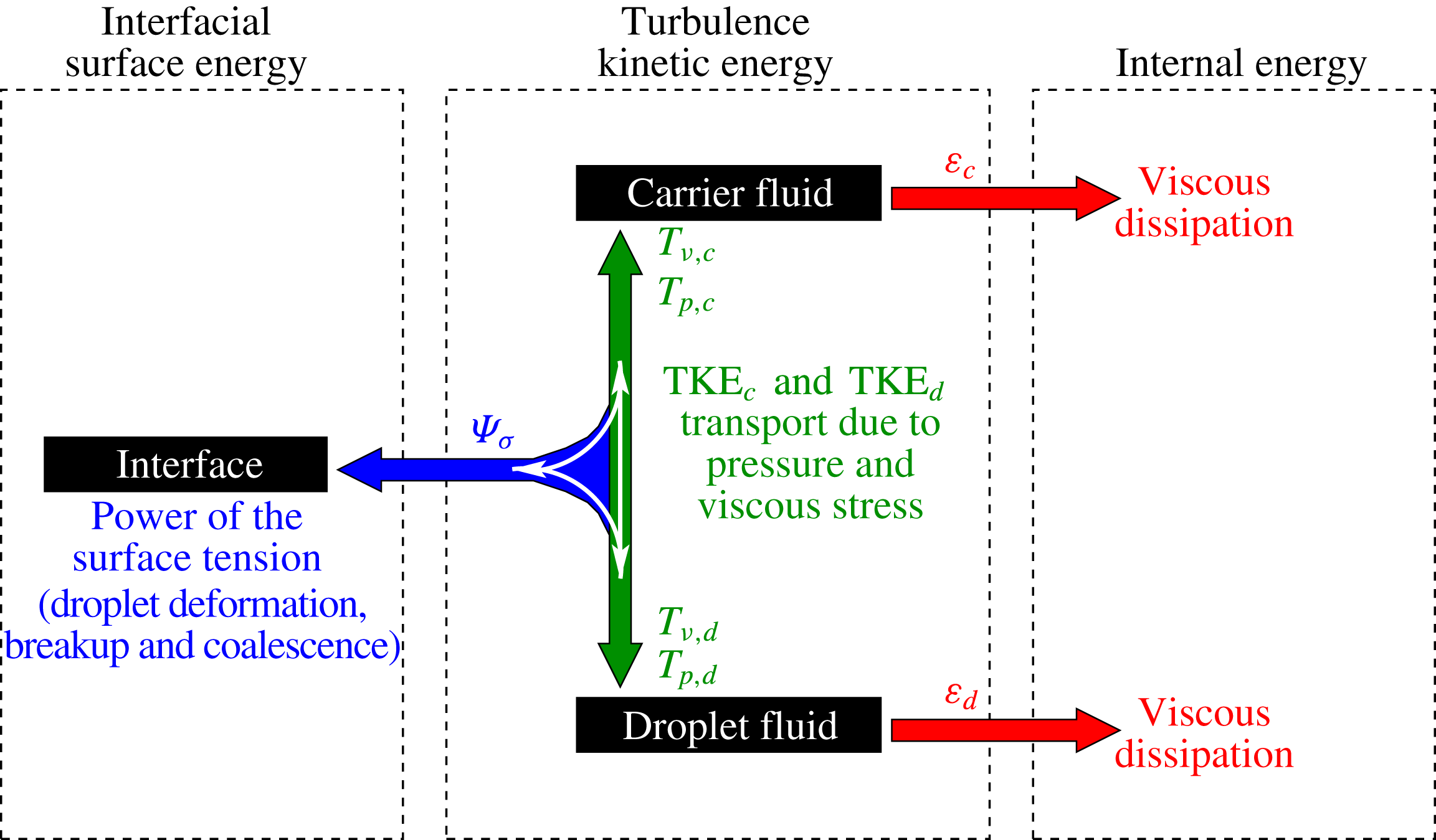
The derived equations, (3.6), (3.8) and (3.9), are summarized schematically in figure 5, which depicts the pathways for TKE exchange in droplet-laden isotropic turbulence, and more generally in two-fluid (liquid–liquid or gas–liquid) isotropic turbulence. All terms responsible for the evolution of
 $k(t)$
(3.6),
 $k_{c}(t)$
(3.8) and
 $k_{d}(t)$
(3.9) are represented. The middle dashed rectangle encompasses the TKE of the two-fluid flow
 $k$
, and shows that the dissipation rate,
 $\unicode[STIX]{x1D700}$
, (red arrows) is a sink of TKE and the power of the surface tension,
 $\unicode[STIX]{x1D6F9}_{\unicode[STIX]{x1D70E}}$
, (blue arrow) is either a source or sink of TKE. The power (or transport) terms
 $T_{\unicode[STIX]{x1D708},c}(t)$
,
 $T_{p,c}(t)$
,
 $T_{\unicode[STIX]{x1D708},d}(t)$
,
 $T_{p,d}(t)$
(green arrows) act to redistribute TKE between the carrier fluid and droplet fluid or into interfacial surface energy via three bidirectional pathways: (i) carrier fluid
 $\leftrightarrow$
droplet fluid (ii) carrier fluid
 $\leftrightarrow$
interface and (iii) droplet fluid
 $\leftrightarrow$
interface (white arrow). This relationship is expressed mathematically by (3.12).
Schematic showing the pathways for TKE exchange in droplet-laden, decaying isotropic turbulence. The dashed rectangles from left to right encompass the interfacial surface energy, TKE, and internal energy. The blue arrow represents TKE being exchanged for interfacial surface energy and vice versa by the power of the surface tension. The green arrow denotes transport of TKE between the two fluids and exchange of TKE for surface energy and vice versa. The red arrows represent TKE of the carrier fluid and droplet fluid being transformed into internal energy by viscous dissipation.

3.3 Comparison of TKE budget for droplet-free and droplet-laden turbulence
In this section, we present the effects of the droplets on turbulence relative to the droplet-free flow by analysing the terms of the TKE budget equation (3.6), and then explain the underlying physical mechanisms.
3.3.1 Two-fluid TKE budget
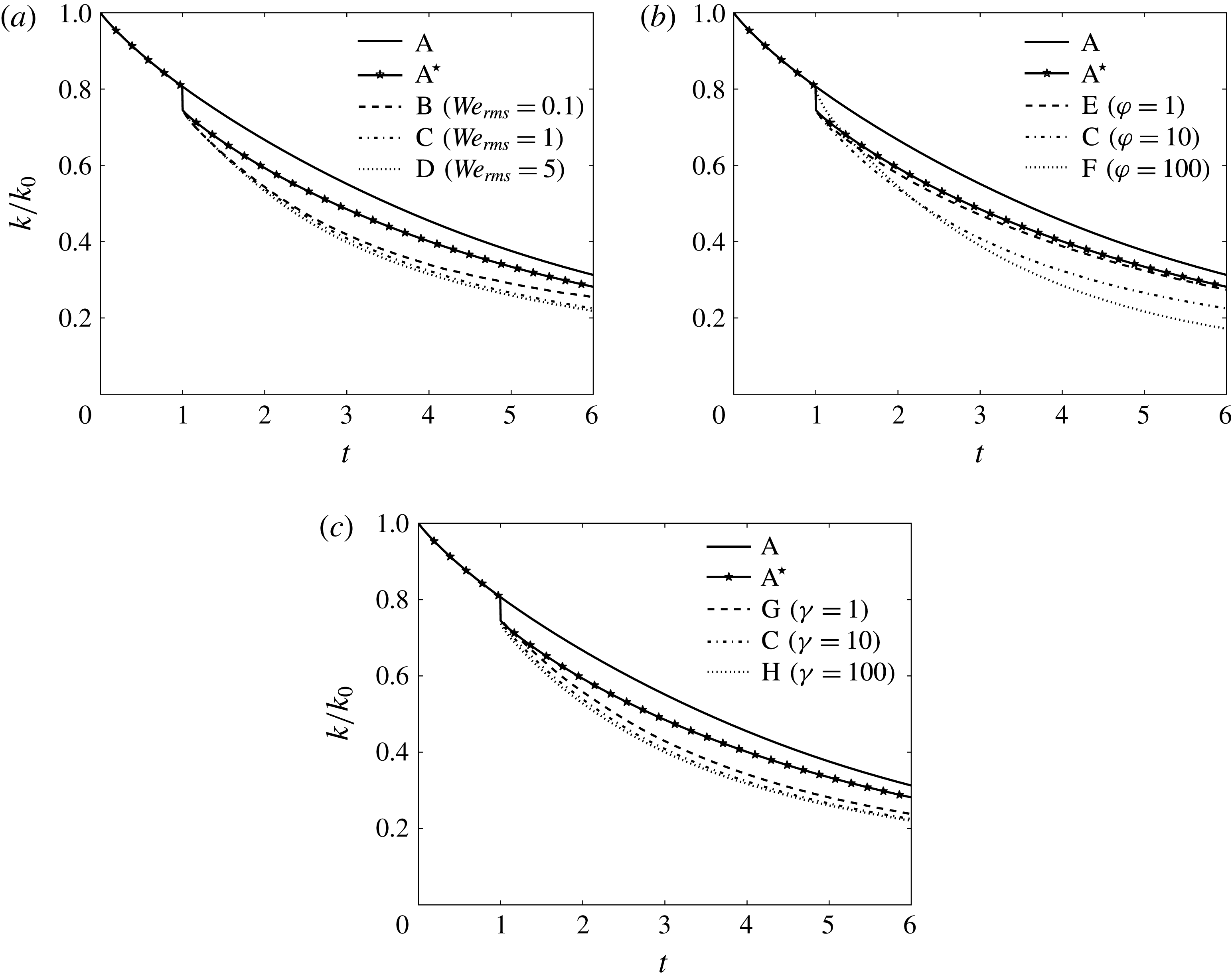
Figure 6 shows the temporal evolution of the turbulence kinetic energy for the two-fluid flow normalized by its initial value,
 $k(t)/k_{0}$
, in cases A–H. When the droplets are introduced (
 $t=1$
),
 $k(t)$
falls by 5 %, corresponding to the volume fraction of fluid that has been set to zero velocity at this time. In all cases
 $\text{A}^{\star }$
–H,
 $k(t)$
remains lower than that in the droplet-free flow (case A).
Temporal evolution of the turbulence kinetic energy,
 $k$
, normalized by its initial value,
 $k_{0}$
.

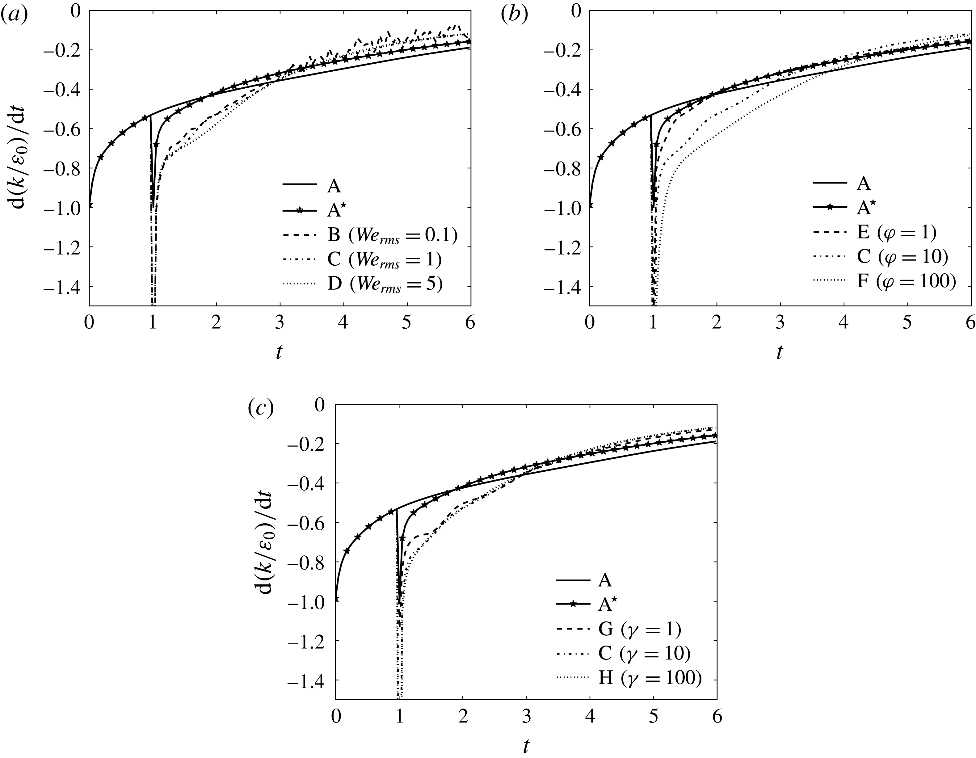
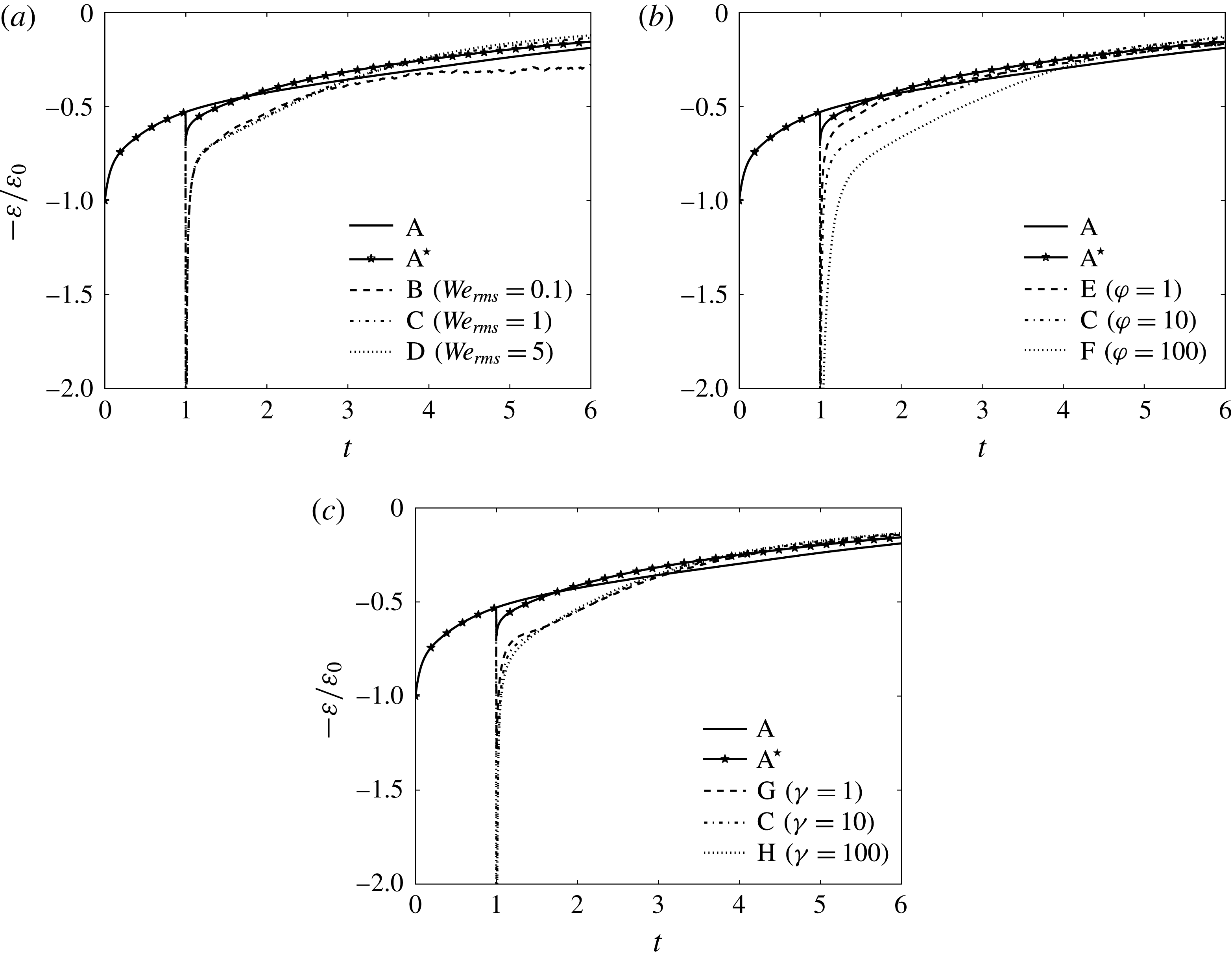
Figure 7 shows the temporal evolution of the rate of change of the TKE normalized by the initial dissipation rate,
 $\text{d}(k(t)/\unicode[STIX]{x1D700}_{0})/\text{d}t$
, in cases A–H. The introduction of the droplets (cases
 $\text{A}^{\star }$
–H) increase the initial decay rate of TKE with respect to that of the single-phase flow (case A). For later times (
 $t>1+\unicode[STIX]{x1D70F}_{\ell }$
), the decay rate of TKE in cases
 $\text{A}^{\star }$
–H stays smaller than that in case A. At early times (
 $1<t<1+\unicode[STIX]{x1D70F}_{\ell }$
), increasing
 $\mathit{We}_{rms}$
(cases B–D),
 $\unicode[STIX]{x1D711}$
(cases E, C and F), or
 $\unicode[STIX]{x1D6FE}$
(cases G, C and H) leads to an increase in the decay rate of TKE. At later times
 $t>1+\unicode[STIX]{x1D70F}_{\ell }$
, the decay rate of TKE is nearly independent of
 $We_{rms}$
(figure 7
a) and
 $\unicode[STIX]{x1D6FE}$
(figure 7
c), but decreases monotonically as
 $\unicode[STIX]{x1D711}$
increases (figure 7
b).
Temporal evolution of the rate of change of turbulence kinetic energy,
 $\text{d}k(t)/\text{d}t$
, normalized by the initial value of the dissipation rate,
 $\unicode[STIX]{x1D700}_{0}$
.

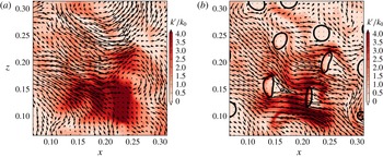
Figure 8 and supplementary movie 1 available at http://dx.doi.org/10.1017/jfm.2016.550 show two-dimensional contours of the local instantaneous kinetic energy (
 $k^{\prime }\equiv (\unicode[STIX]{x1D70C}u_{j}u_{j})/2$
) and the fluid velocity vectors (
 $u_{j}$
) in a subregion of the computational domain in cases A and C at
 $t=1.5$
, which corresponds to approximately one Taylor time scale after droplet release (
 $t\approx 1+\unicode[STIX]{x1D70F}_{\unicode[STIX]{x1D706}}$
). Comparing figures 8(a) and 8(b), we note that in 8(b) (case C) there are less regions of high
 $k^{\prime }$
(red regions), particularly in the droplet wake. Also, inside the droplets,
 $k^{\prime }>0^{\prime }$
, which denotes an increase because the droplets were initially released from rest. This is consistent with
 $k$
being lower in cases
 $\text{A}^{\star }$
–H than it is in case A because
 $k=\langle k^{\prime }\rangle$
.
Instantaneous contours in a subregion of the
 $x{-}z$
plane of
 $k^{\prime }=(\unicode[STIX]{x1D70C}u_{j}u_{j})/2$
in (a) case A and (b) case C at
 $t=1.5$
. The black arrows are the instantaneous velocity vectors projected onto the
 $x{-}z$
plane.

To explain why droplets enhance the decay rate of
 $k(t)$
, we analyse the temporal evolution of the terms on the right-hand side of (3.6), that is
 $\unicode[STIX]{x1D700}(t)$
and
 $\unicode[STIX]{x1D6F9}_{\unicode[STIX]{x1D70E}}(t)$
(represented by red and blue arrows in figure 5). Figure 9 shows the temporal evolution of the normalized dissipation rate of TKE for the two-fluid flow,
 $\unicode[STIX]{x1D700}(t)/\unicode[STIX]{x1D700}_{0}$
. When droplets are introduced into the flow (cases
 $\text{A}^{\star }$
–H) at
 $t=1$
,
 $\unicode[STIX]{x1D700}(t)$
spikes relative to that of case A. At
 $t\approx 1+\unicode[STIX]{x1D70F}_{\ell }$
,
 $\unicode[STIX]{x1D700}(t)$
in cases
 $\text{A}^{\star }$
–H crosses over that of case A. The crossover of
 $\unicode[STIX]{x1D700}(t)$
at
 $t\approx 1+\unicode[STIX]{x1D70F}_{\ell }$
(except for in case
 $\text{A}^{\star }$
and B) occurs because
 $k(t)$
in the droplet-laden cases at later times is less than
 $k(t)$
of the droplet-free case (A), and therefore, the dissipation rate of
 $k(t)$
is also lower. Furthermore, figures 9(a) and 9(c) show that, for early times (
 $1<t<1+\unicode[STIX]{x1D70F}_{\ell }$
),
 $\unicode[STIX]{x1D700}(t)$
is approximately independent of
 $\mathit{We}_{rms}$
and
 $\unicode[STIX]{x1D6FE}$
for the range of values tested, whereas figure 9(b) shows that
 $\unicode[STIX]{x1D700}(t)$
increases monotonically with increasing
 $\unicode[STIX]{x1D711}$
. For longer times (
 $t>1+\unicode[STIX]{x1D70F}_{\ell }$
), figure 9(a) shows that
 $\unicode[STIX]{x1D700}(t)$
in case B is higher than that in cases C and D, eventually having twice the magnitude at
 $t=6$
. Figure 9(b) shows that
 $\unicode[STIX]{x1D700}(t)$
in cases C and F crosses over that of E, which is a result of
 $\text{d}k(t)/\text{d}t$
being higher for (
 $t<1+\unicode[STIX]{x1D70F}_{\ell }$
) in cases C and F (see figure 7
b). Figure 9(c) shows that
 $\unicode[STIX]{x1D700}(t)$
remains nearly independent of
 $\unicode[STIX]{x1D6FE}$
for
 $1\leqslant t\leqslant 6$
.
Temporal evolution of the dissipation rate of turbulence kinetic energy,
 $\unicode[STIX]{x1D700}$
, normalized by its initial value,
 $\unicode[STIX]{x1D700}_{0}$
.

The power of the surface tension,
 $\unicode[STIX]{x1D6F9}_{\unicode[STIX]{x1D70E}}(t)$
, is zero in cases A and
 $\text{A}^{\star }$
(
 $\boldsymbol{f}_{\unicode[STIX]{x1D70E}}=0\rightarrow \unicode[STIX]{x1D6F9}_{\unicode[STIX]{x1D70E}}=0$
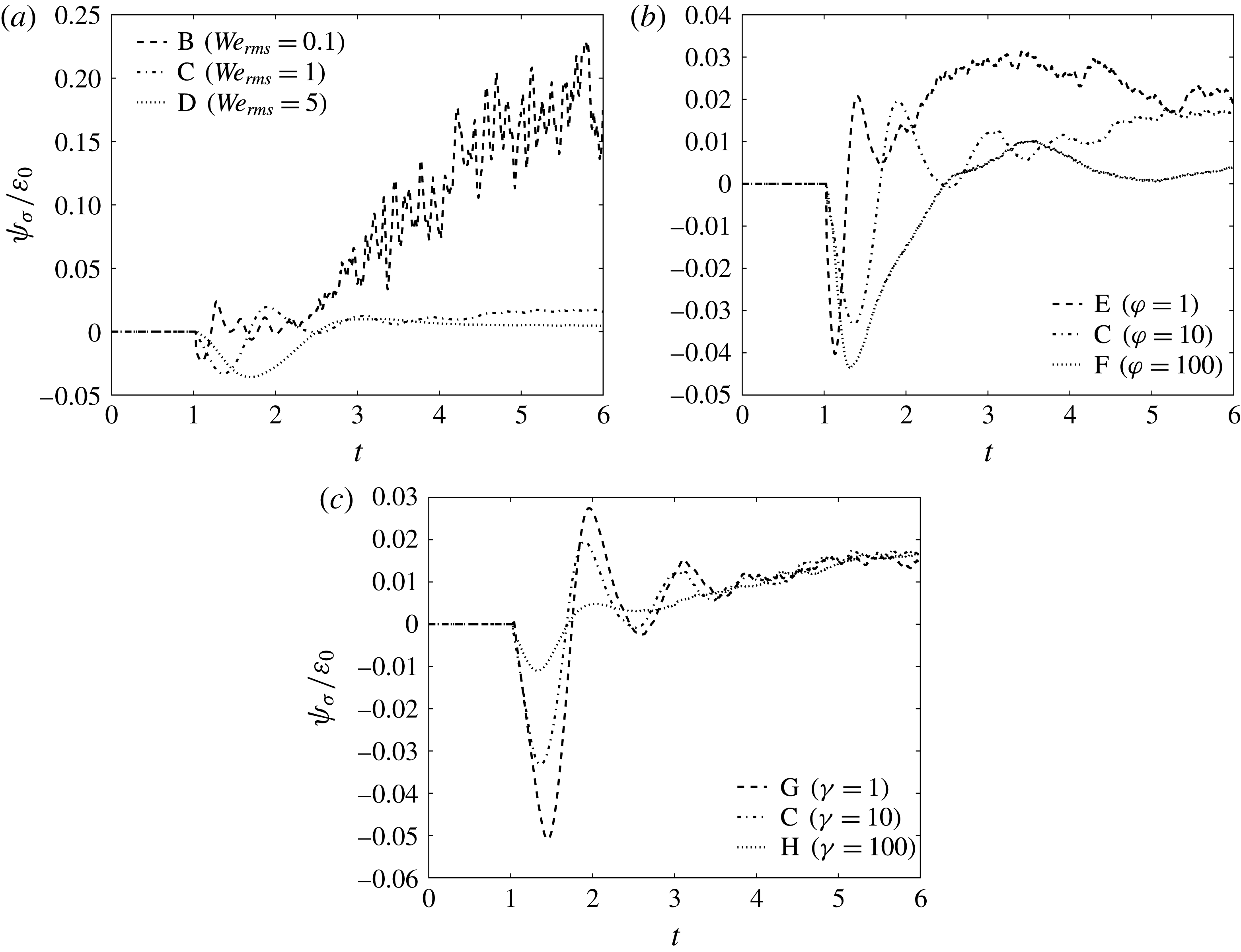
) and positive or negative in droplet-laden cases with finite Weber number (B–H), as shown in figure 10. In all cases
 $\unicode[STIX]{x1D6F9}_{\unicode[STIX]{x1D70E}}(t)$
is initially negative, and the magnitude of the peak increases monotonically for increasing
 $\mathit{We}_{rms}$
or decreasing
 $\unicode[STIX]{x1D6FE}$
, whereas it is non-monotonic and nearly independent for increasing
 $\unicode[STIX]{x1D711}$
. In general,
 $\unicode[STIX]{x1D6F9}_{\unicode[STIX]{x1D70E}}(t)$
tends to oscillate about
 $\unicode[STIX]{x1D6F9}_{\unicode[STIX]{x1D70E}}(t)=0$
for early times (
 $t<1+\unicode[STIX]{x1D70F}_{\ell }$
), which leads to oscillations in the TKE decay rate that are most noticeable in cases B, C and G (figure 7). For
 $t>1+\unicode[STIX]{x1D70F}_{\ell }$
,
 $\unicode[STIX]{x1D6F9}_{\unicode[STIX]{x1D70E}}(t)$
is strictly positive, and therefore, the power of the surface tension is a source of TKE. In all cases,
 $\unicode[STIX]{x1D6F9}_{\unicode[STIX]{x1D70E}}(t)$
is limited to
 $\pm 5\,\%$
of
 $\unicode[STIX]{x1D700}_{0}$
, for
 $t<1+\unicode[STIX]{x1D70F}_{\ell }$
, and consequently it plays a neutral role in the time evolution of the TKE for early times. Rather,
 $\unicode[STIX]{x1D6F9}_{\unicode[STIX]{x1D70E}}(t)$
plays a more important role for
 $t>1+\unicode[STIX]{x1D70F}_{\ell }$
, where it behaves as a source of TKE, especially in case B.
Temporal evolution of the power of the surface tension,
 $\unicode[STIX]{x1D6F9}_{\unicode[STIX]{x1D70E}}$
, normalized by the initial value of the dissipation rate,
 $\unicode[STIX]{x1D700}_{0}$
.

Figure 10 shows that, for
 $\mathit{We}_{rms}=0.1$
(case B),
 $\unicode[STIX]{x1D6F9}_{\unicode[STIX]{x1D70E}}(t=6)$
is roughly 20 % of the initial dissipation rate,
 $\unicode[STIX]{x1D700}_{0}$
, which corresponds to 50 % of the instantaneous dissipation rate,
 $\unicode[STIX]{x1D700}(t=6)$
, thus representing a significant source of TKE in (3.6). The enhanced power of the surface tension (
 $\unicode[STIX]{x1D6F9}_{\unicode[STIX]{x1D70E}}>0$
) is accompanied by enhanced dissipation,
 $\unicode[STIX]{x1D700}(t)$
, relative to cases C and D, such that
 $\text{d}k(t)/\text{d}t$
in case B is nearly equivalent to that in cases C and D, as was seen in figure 6(a).
In summary, the results show that, for early times,
 $1<t<1+\unicode[STIX]{x1D70F}_{\ell }$
, the droplets enhance the decay rate of TKE,
 $\text{d}k(t)/\text{d}t$
(figure 7), relative to the droplet-free flow, and that this is due almost entirely to the enhanced dissipation rate of TKE,
 $\unicode[STIX]{x1D700}(t)$
(figure 9). The power of the surface tension,
 $\unicode[STIX]{x1D6F9}_{\unicode[STIX]{x1D70E}}(t)$
(figure 10), is limited to
 $\pm 5\,\%$
of
 $\unicode[STIX]{x1D700}_{0}$
, for
 $t<2.5$
, and consequently it plays a minor role in the early development of
 $k(t)$
. For later times,
 $t>1+\unicode[STIX]{x1D70F}_{\ell }$
,
 $\unicode[STIX]{x1D6F9}_{\unicode[STIX]{x1D70E}}(t)$
plays a more important role, behaving as a source term with magnitude of up to 50 % of
 $\unicode[STIX]{x1D700}(t)$
(case B).
3.3.2 Dissipation rate of TKE
To explain why
 $\unicode[STIX]{x1D700}(t)$
is greater in cases
 $\text{A}^{\star }$
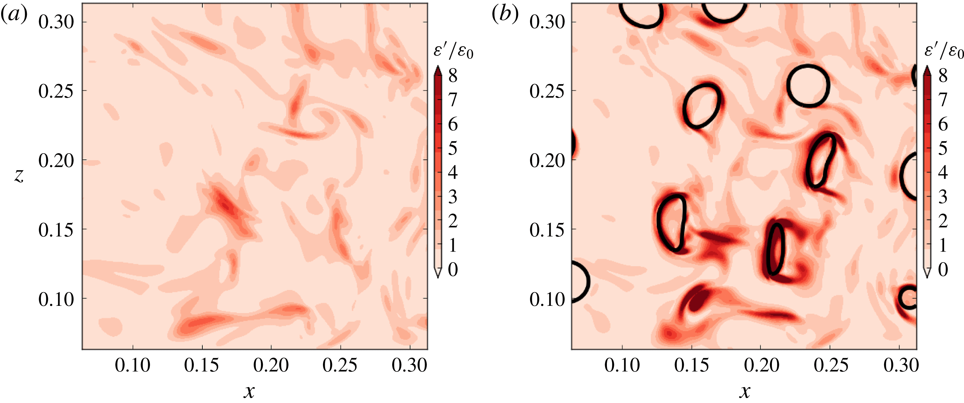
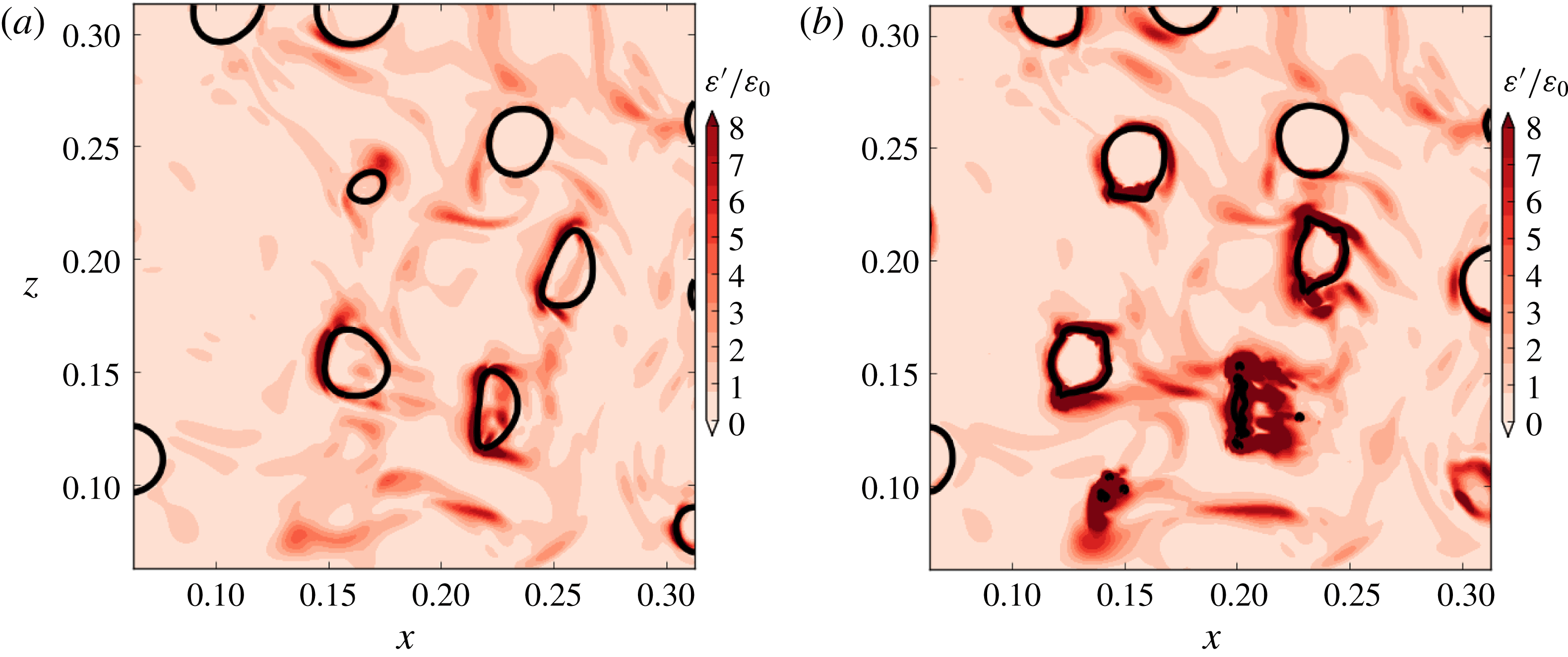
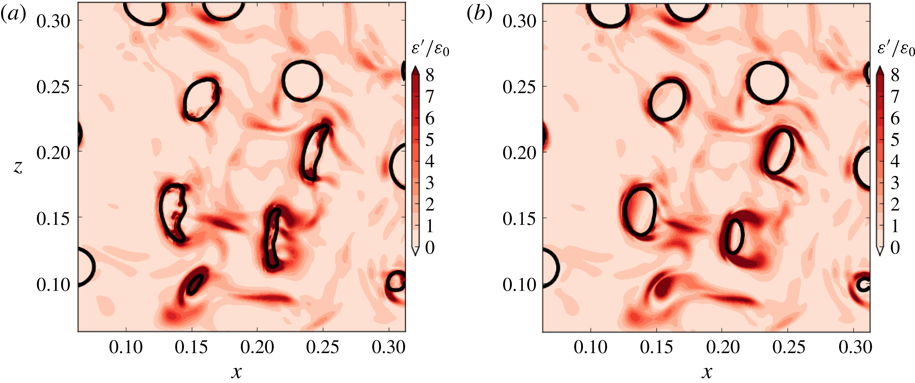
–H than in case A, figure 11 and supplementary movie 2 show the instantaneous two-dimensional contours of
 $\unicode[STIX]{x1D700}^{\prime }\equiv \mathit{Re}^{-1}(\unicode[STIX]{x1D61B}_{ij}\unicode[STIX]{x1D61A}_{ij})$
in a subregion of the computational domain at
 $t=1.5$
in cases A and C. Figure 11(b) shows that
 $\unicode[STIX]{x1D700}^{\prime }$
is enhanced near the droplet surface. The increased
 $\unicode[STIX]{x1D700}^{\prime }$
near the droplet interface is due to the local increase of
 $\unicode[STIX]{x1D61A}_{ij}$
, which is due to the increase of the velocity gradient (
 $\unicode[STIX]{x2202}u_{i}/\unicode[STIX]{x2202}x_{j}$
) near the droplet interface. The increase in
 $\unicode[STIX]{x2202}u_{i}/\unicode[STIX]{x2202}x_{j}$
is caused by (i) the velocity being set to zero in the droplet interiors at
 $t=1$
(compare
 $\unicode[STIX]{x1D700}(t)$
case A to cases
 $\text{A}^{\star }$
–H), (ii) finite Weber number effects (compare
 $\unicode[STIX]{x1D700}(t)$
case
 $\text{A}^{\star }$
to cases B–H) and (iii) the droplet trajectories deviating from the motion of the carrier fluid in cases in which the droplets are more dense than the carrier fluid (cases B, C, D, F, G and H). The trajectories deviate more because of the higher inertia of the droplets compared to that of the carrier-fluid turbulence eddies (both large and small scales of motion), because the droplet Stokes numbers, based on both the integral time scale and on the Kolmogorov time scale, are much larger than unity,
 $St_{\ell }=\unicode[STIX]{x1D70F}_{d}/\unicode[STIX]{x1D70F}_{\ell }=15.8$
and
 $St_{\unicode[STIX]{x1D702}}=\unicode[STIX]{x1D70F}_{d}/\unicode[STIX]{x1D70F}_{\unicode[STIX]{x1D702}}=225$
, respectively. Finally, the local increase of
 $\unicode[STIX]{x1D700}^{\prime }$
increases
 $\unicode[STIX]{x1D700}(t)$
because
 $\unicode[STIX]{x1D700}(t)=\langle \unicode[STIX]{x1D700}^{\prime }\rangle$
.
Instantaneous contours in a subregion of the
 $x{-}z$
plane of
 $\unicode[STIX]{x1D700}^{\prime }=\mathit{Re}^{-1}(\unicode[STIX]{x1D61B}_{ij}\unicode[STIX]{x1D61A}_{ij})$
in (a) case A and (b) case C at
 $t=1.5$
.

In § 3.3.1 it was shown that, for
 $1<\unicode[STIX]{x1D70F}_{\ell }<1+\unicode[STIX]{x1D70F}_{\ell }$
, as
 $\mathit{We}_{rms}$
and
 $\unicode[STIX]{x1D6FE}$
are varied,
 $\unicode[STIX]{x1D700}(t)$
is nearly constant, but as
 $\unicode[STIX]{x1D711}$
increases,
 $\unicode[STIX]{x1D700}(t)$
increases (figure 9
b). As
 $\unicode[STIX]{x1D711}$
increases, the droplet inertia increases. For example, the droplet Stokes number (
 $\unicode[STIX]{x1D70F}_{d}/\unicode[STIX]{x1D70F}_{\ell }$
) for
 $\unicode[STIX]{x1D711}=100$
(case F) is 100 times greater than that for
 $\unicode[STIX]{x1D711}=1$
(case E) (table 2). As the droplet inertia increases, the trajectories of the droplets compared to those of the surrounding fluid deviate more, which leads to higher velocity gradients (
 $\unicode[STIX]{x2202}u_{i}/\unicode[STIX]{x2202}x_{j}$
), and therefore, enhanced
 $\unicode[STIX]{x1D700}^{\prime }$
near the droplet interface. This can be seen by comparing contours of
 $\unicode[STIX]{x1D700}^{\prime }$
in cases E (
 $\unicode[STIX]{x1D70F}_{d}/\unicode[STIX]{x1D70F}_{\ell }=1.58$
) and F (
 $\unicode[STIX]{x1D70F}_{d}/\unicode[STIX]{x1D70F}_{\ell }=158$
), as shown in figure 12 at
 $t=1.5$
and supplementary movie 3.
Instantaneous contours in a subregion of the
 $x{-}z$
plane of
 $\unicode[STIX]{x1D700}^{\prime }=\mathit{Re}^{-1}(\unicode[STIX]{x1D61B}_{ij}\unicode[STIX]{x1D61A}_{ij})$
in (a) case E and (b) case F at
 $t=1.5$
.

3.3.3 Power of the surface tension
In § 3.3.1, the results have shown that the power of the surface tension can act as a source or sink of TKE. We now explain in more detail the behaviour of
 $\unicode[STIX]{x1D6F9}_{\unicode[STIX]{x1D70E}}(t)$
, and why it changes for varying
 $\mathit{We}_{rms}$
,
 $\unicode[STIX]{x1D711}$
and
 $\unicode[STIX]{x1D6FE}$
.
Physically, the power of the surface tension,
 $\unicode[STIX]{x1D6F9}_{\unicode[STIX]{x1D70E}}(t)$
, represents the rate of change of the surface energy of the droplet interface. In appendix C, we derive the following relationship between
 $\unicode[STIX]{x1D6F9}_{\unicode[STIX]{x1D70E}}(t)$
and the rate of change of the total droplet surface area
 $\text{d}A(t)/\text{d}t$
,
 $$\begin{eqnarray}\unicode[STIX]{x1D6F9}_{\unicode[STIX]{x1D70E}}(t)=-\frac{1}{\mathit{We}}\frac{1}{\mathscr{V}}\frac{\text{d}A(t)}{\text{d}t},\end{eqnarray}$$
where
 $\mathscr{V}$
is the volume of the domain (
 $\mathscr{V}=1$
) and
 $A(t)$
is the total droplet surface area defined as
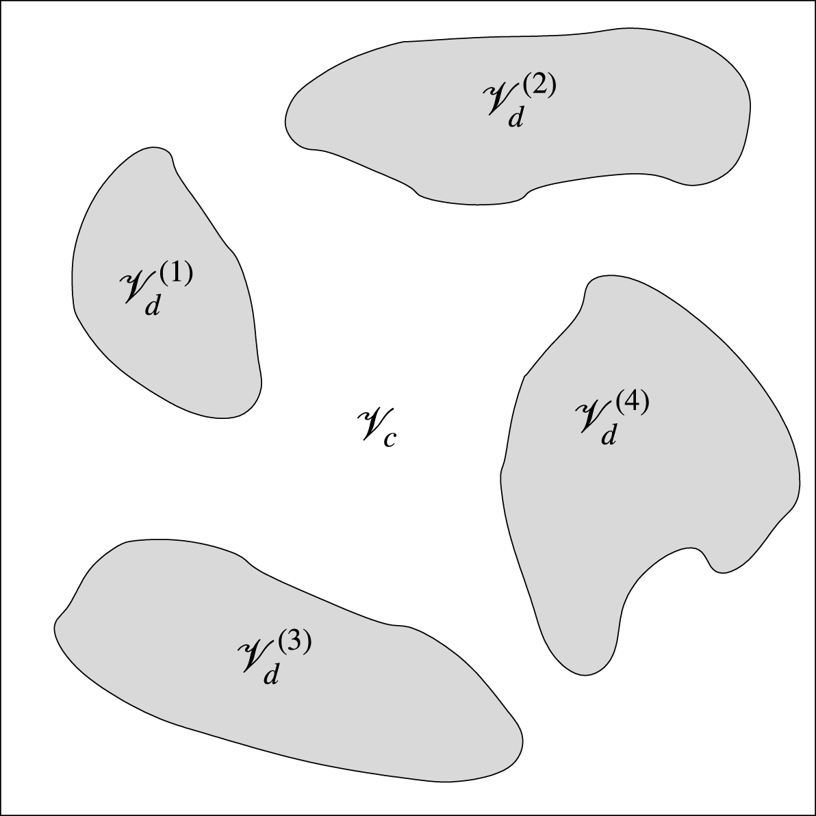
 $$\begin{eqnarray}A(t)\equiv \mathop{\sum }_{n=1}^{N_{d}(t)}\iint _{\unicode[STIX]{x2202}\mathscr{V}_{c}^{(n)}(t)}\text{d}\mathscr{A}=\mathop{\sum }_{n=1}^{N_{d}(t)}A^{(n)}(t),\end{eqnarray}$$
where
 $N_{d}(t)$
is the instantaneous number of droplets,
 $\unicode[STIX]{x2202}\mathscr{V}_{c}^{(n)}(t)$
is the instantaneous control surface that bounds the
 $n$
th droplet interface from the carrier-fluid side and
 $A^{(n)}(t)$
is the instantaneous surface area of the
 $n$
th droplet.
 $\unicode[STIX]{x1D6F9}_{\unicode[STIX]{x1D70E}}(t)$
is directly proportional to the rate of change of droplet surface area (with opposite sign) and the constant of proportionality is the non-dimensional surface tension coefficient
 $\mathit{We}$
. For example, an increase in droplet surface area in time (
 $\text{d}A(t)/\text{d}t>0$
), indicates through (3.13) that
 $\unicode[STIX]{x1D6F9}_{\unicode[STIX]{x1D70E}}(t)<0$
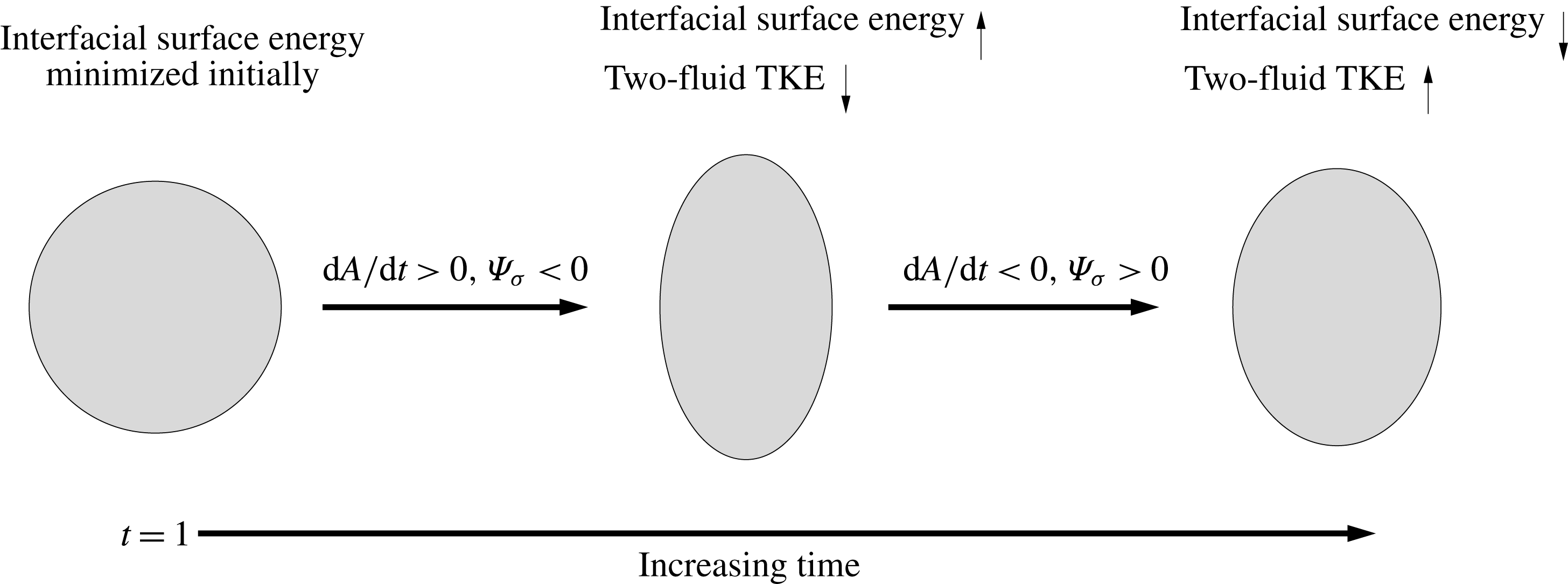
, i.e. the droplets act as a sink of TKE by accumulating energy as droplet interfacial surface energy. We highlight this as a key concept for analysing the energy budget of turbulent flows laden with deformable droplets (figures 5 and 13).
Schematic of a droplet oscillating in its fundamental mode that illustrates one of the physical mechanisms of the power of the surface tension (
 $\unicode[STIX]{x1D6F9}_{\unicode[STIX]{x1D70E}}(t)=\mathit{We}^{-1}\mathscr{V}^{-1}(\text{d}A(t)/\text{d}t)$
). Going from left to right, the surface energy increases (two-fluid TKE decreases) as the droplet surface area increases, and then the surface energy decreases (two-fluid TKE increases) as the droplet surface area decreases (3.13).

At
 $t=1$
the droplets are spherical, corresponding to
 $A(t)$
being minimized, and therefore, immediately after the droplets are released, it must be true that
 $\text{d}A(t)/\text{d}t\geqslant 0$
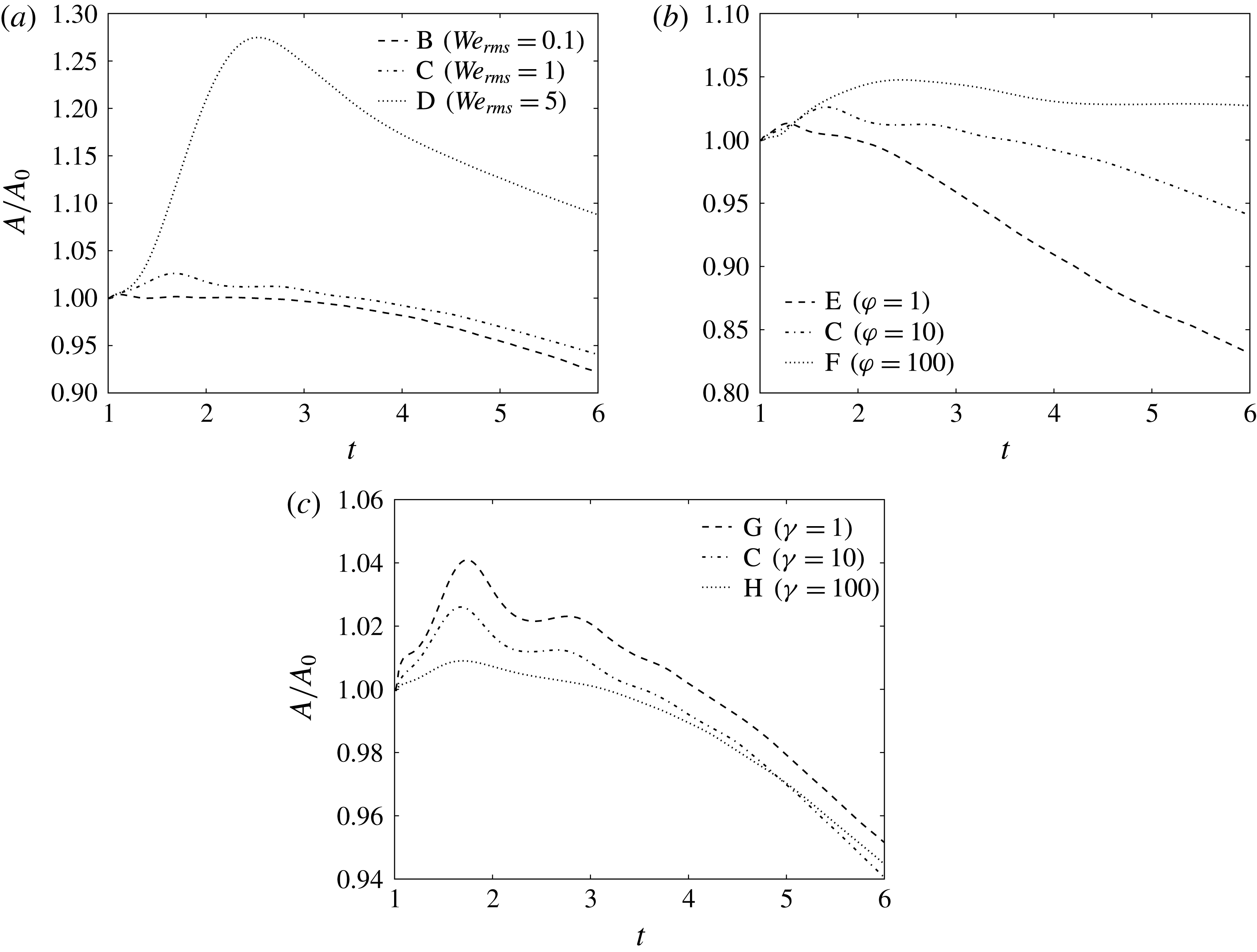
(figure 13). Figure 14 confirms that
 $A$
initially grows in time (i.e.
 $\text{d}A(t)/\text{d}t>0$
), which, from (3.13), corresponds to
 $\unicode[STIX]{x1D6F9}_{\unicode[STIX]{x1D70E}}(t)<0$
(figure 10). Figure 14 shows that, initially, the surface area growth rate,
 $\text{d}A(t)/\text{d}t$
, increases monotonically with increasing
 $\mathit{We}_{rms}$
or decreasing
 $\unicode[STIX]{x1D6FE}$
, and is non-monotonic for increasing
 $\unicode[STIX]{x1D711}$
.
Temporal evolution of the total surface area of the droplets normalized by its initial value,
 $A(t)/A_{0}$
.

In § 3.3.3, we saw from figure 10 that
 $\unicode[STIX]{x1D6F9}_{\unicode[STIX]{x1D70E}}(t)$
tends to oscillate for early times (
 $1<t<2.5$
). At
 $t=1$
, the droplets are subjected to immediate aerodynamic forces from the carrier fluid, which leads to the droplets oscillating in unison on average, i.e. periods when
 $\text{d}A(t)/\text{d}t>0$
and
 ${<}0$
. Because
 $\unicode[STIX]{x1D6F9}_{\unicode[STIX]{x1D70E}}(t)$
is directly proportional to
 $\text{d}A(t)/\text{d}t$
(via (3.13)), oscillations in
 $\text{d}A(t)/\text{d}t$
lead to oscillations in
 $\unicode[STIX]{x1D6F9}_{\unicode[STIX]{x1D70E}}(t)$
. Figure 13 depicts a single droplet system undergoing oscillations. The period of oscillation corresponds to the fundamental vibrational mode of the droplets in the inviscid limit (Frohn & Roth Reference Frohn and Roth2000), which in non-dimensional form is
 $$\begin{eqnarray}T_{\mathit{dvm}}=\frac{\unicode[STIX]{x03C0}}{4}\sqrt{\frac{D^{2}\mathit{ We }_{rms}(3\unicode[STIX]{x1D711}+2)}{3U_{rms}^{2}}}.\end{eqnarray}$$
(The period of the droplet fundamental vibrational mode in dimensional form is
 $\tilde{T}_{\mathit{dvm}}=\unicode[STIX]{x03C0}/4\sqrt{\tilde{D}^{3}(3\tilde{\unicode[STIX]{x1D70C}}_{d}+2\tilde{\unicode[STIX]{x1D70C}}_{c})/3\tilde{\unicode[STIX]{x1D70E}}}$
.)
 $T_{\mathit{dvm}}$
is reported in table 3 for cases B–H. In case B, the oscillations are a superposition of the fundamental and the second vibrational mode. Equation (3.15) shows that
 $T_{\mathit{dvm}}$
increases with increasing
 $\mathit{We}_{rms}$
and
 $\unicode[STIX]{x1D711}$
, and is independent of
 $\unicode[STIX]{x1D6FE}$
, which is consistent with the behaviour of
 $\unicode[STIX]{x1D6F9}_{\unicode[STIX]{x1D70E}}(t)$
seen in figure 10.


An additional phenomenon during the droplet oscillations is that TKE is lost irreversibly due to viscous dissipation, which damps
 $\text{d}A(t)/\text{d}t$
(see figure 10). The non-dimensional number which characterizes the degree to which TKE is lost due to viscous dissipation during the droplet oscillations is the Ohnesorge number,
 $$\begin{eqnarray}Oh=\frac{\tilde{\unicode[STIX]{x1D707}}_{d}}{\sqrt{\tilde{\unicode[STIX]{x1D70C}}_{d}\tilde{\unicode[STIX]{x1D70E}}\tilde{D}}}=\frac{\unicode[STIX]{x1D6FE}\sqrt{\mathit{We }_{rms}}}{DU_{rms}\mathit{Re}\sqrt{\unicode[STIX]{x1D711}}},\end{eqnarray}$$
which is the ratio of the viscous force to the square root of the product of the inertial and surface tension forces. Table 3 shows
 $Oh$
in all droplet-laden cases B–H. Table 3 and (3.16) show that
 $Oh$
increases with increasing
 $\mathit{We}_{rms}$
, decreasing
 $\unicode[STIX]{x1D711}$
or increasing
 $\unicode[STIX]{x1D6FE}$
. As
 $Oh$
increases, the droplet surface area oscillations in time (
 $\text{d}A(t)/\text{d}t$
) are damped more quickly by viscous forces, and therefore, from (3.13), the oscillations in
 $\unicode[STIX]{x1D6F9}_{\unicode[STIX]{x1D70E}}(t)$
are also damped more quickly. This explains why the oscillations in
 $\unicode[STIX]{x1D6F9}_{\unicode[STIX]{x1D70E}}(t)$
are more damped for increasing
 $\mathit{We}_{rms}$
, decreasing
 $\unicode[STIX]{x1D711}$
or increasing
 $\unicode[STIX]{x1D6FE}$
, as seen in figure 10.
We now explain why
 $\unicode[STIX]{x1D6F9}_{\unicode[STIX]{x1D70E}}(t)$
is strictly positive for longer times. For
 $t>1+\unicode[STIX]{x1D70F}_{\ell }$
, the droplets surface area,
 $A(t)$
, tends to decrease in time (
 $\text{d}A(t)/\text{d}t<0$
), which leads to
 $\unicode[STIX]{x1D6F9}_{\unicode[STIX]{x1D70E}}(t)>0$
(via (3.13)). It is also interesting to note that at
 $t=6$
,
 $A(t)/A_{0}<1$
in cases B, C, E, G and H. The only mechanism that can cause
 $A(t)<A_{0}$
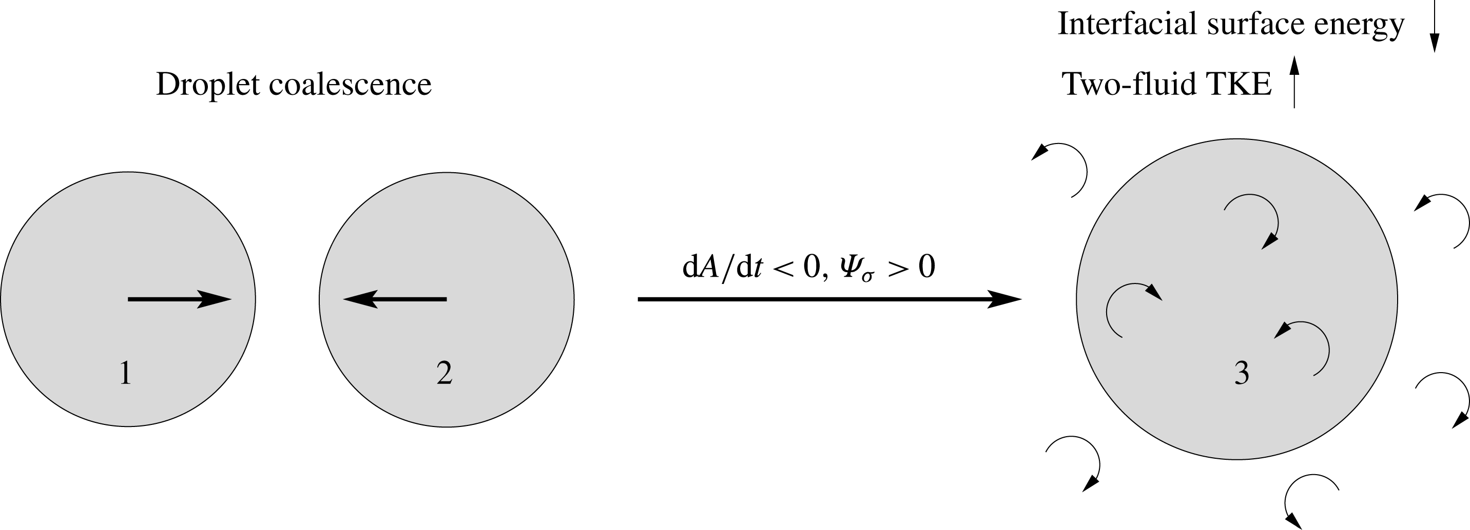
in the present flow is droplet coalescence. To demonstrate this, consider the simplified case of two equally sized spherical droplets coalescing to form a larger spherical droplet, as illustrated in figure 15. In this case, the total surface area of the droplet fluid decreases by 21 %. Therefore, during coalescence, a fraction of the surface energy stored in the interface is transformed into TKE (blue
 $\rightarrow$
green pathway in figure 5). This process is reversed during breakup, in which the total droplet surface area increases (
 $\text{d}A(t)/\text{d}t>0$
), leading to negative power of the surface tension (
 $\unicode[STIX]{x1D6F9}_{\unicode[STIX]{x1D70E}}(t)<0$
).
Schematic of two spherical droplets with the same diameter and surface area (
 $A^{(1)}=A^{(2)}$
) coalescing to form a larger spherical droplet with surface area
 $A^{(3)}$
. The surface area of the new droplet
 $A^{(3)}$
is 21 % less than that of the two original droplets
 $2A^{(1)}$
(i.e.
 $A^{(3)}/(2A^{(1)})=0.79$
). More generally, droplet coalescence is associated with
 $\text{d}A(t)/\text{d}t<0$
, and thus
 $\unicode[STIX]{x1D6F9}_{\unicode[STIX]{x1D70E}}(t)>0$
(3.13). This process is reversed during droplet breakup for which
 $\text{d}A(t)/\text{d}t>0$
and
 $\unicode[STIX]{x1D6F9}_{\unicode[STIX]{x1D70E}}(t)<0$
.

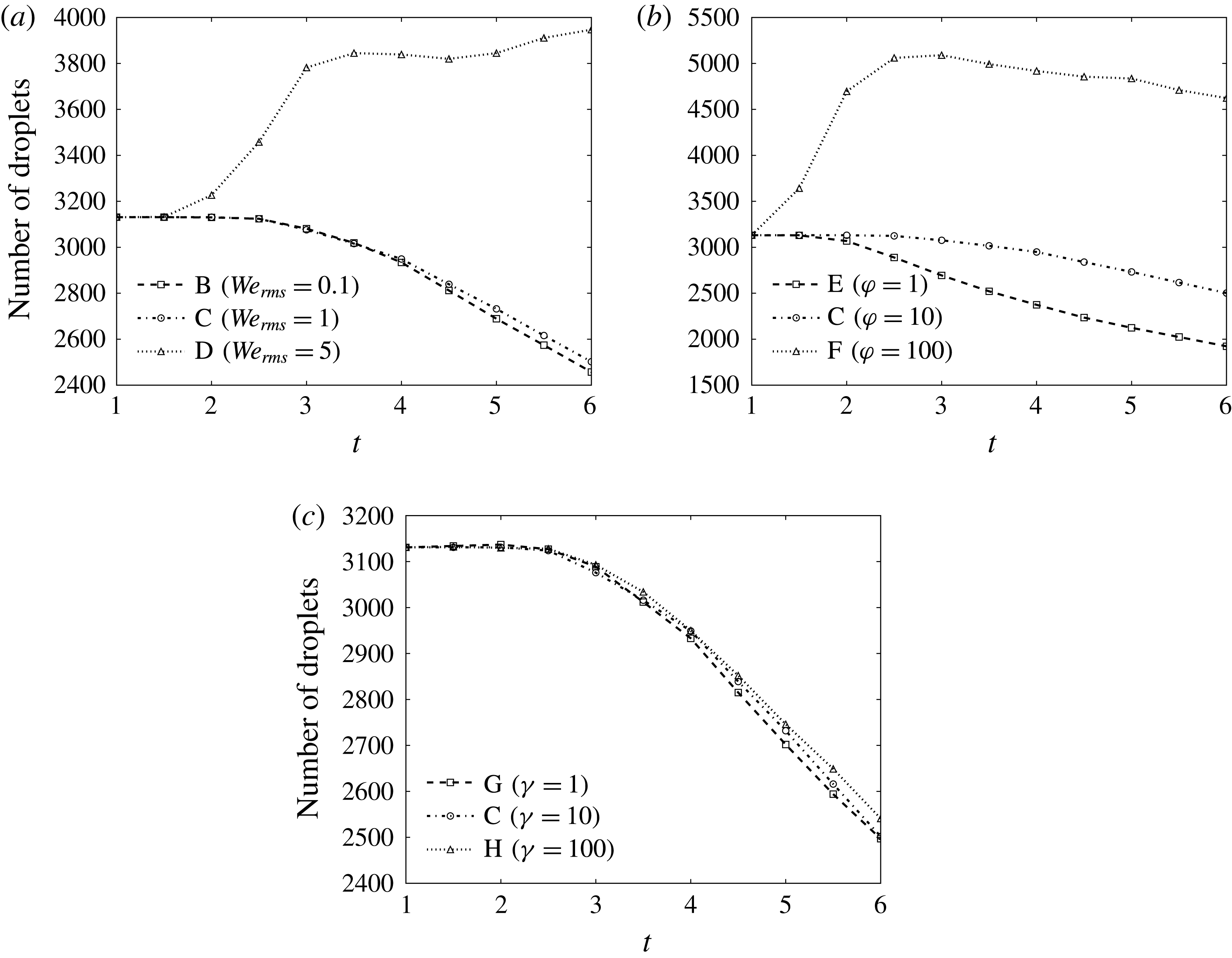
To quantify the rate of droplet coalescence we compute the number of droplets in the computational domain as a function of time. Figure 16 shows that, in cases B, C, E, G and H, the number of droplets decreases in time, indicating that droplets are coalescing. The onset of droplet coalescence, e.g. at
 $t\approx 2.5$
in case B, leads to fluctuations in
 $\unicode[STIX]{x1D6F9}_{\unicode[STIX]{x1D70E}}(t)$
, as the droplets no longer oscillate in unison with period
 $T_{\mathit{dvm}}$
, but instead coalesce at different times as they are driven by the turbulent eddies, and will have a period of oscillation greater than
 $T_{\mathit{dvm}}$
. At
 $t=6$
the number of droplets increases with increasing
 $\mathit{We}_{rms}$
,
 $\unicode[STIX]{x1D711}$
or
 $\unicode[STIX]{x1D6FE}$
. Figure 16 shows that in cases D and F, the number of droplets increases to a value greater than the initial value, which denotes that the number of breakups exceeds the number of coalescences.
Number of droplets in the computational domain as a function of time in cases B–H.

To better quantify the number of coalescence and breakup events, the droplet size distribution is computed. We calculate the equivalent spherical diameter of each droplet in the domain as
 $$\begin{eqnarray}D^{(n)}=(6\mathscr{V}_{d}^{(n)}/\unicode[STIX]{x03C0})^{1/3},\end{eqnarray}$$
where
 $\mathscr{V}_{d}^{(n)}$
is the volume of the
 $n$
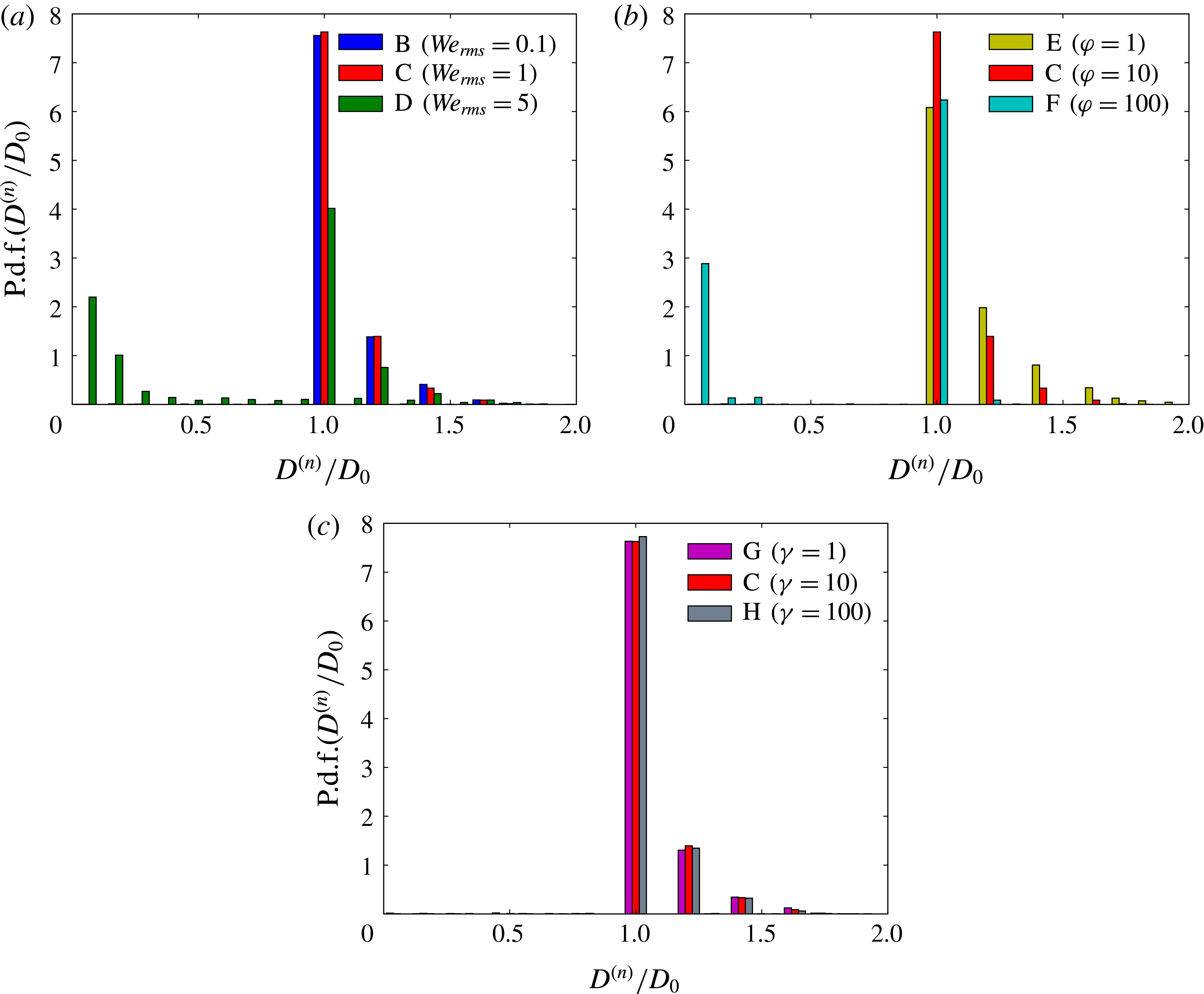
th droplet. Figure 17 shows the probability density function of the equivalent spherical diameter
 $D^{(n)}$
normalized by its initial value
 $D_{0}$
in cases B–H at
 $t=6$
.
 $D^{(n)}/D_{0}>1$
(
 $D^{(n)}/D_{0}<1$
) indicates that the droplet equivalent spherical diameter has increased (decreased), and thus indicates an instance of coalescence (breakup). Figure 17 shows that in all cases, except in case F, that some of the droplets have coalesced in groups of two to four, and that as
 $D^{(n)}/D_{0}$
increases, the probability density of
 $D^{(n)}/D_{0}$
decreases.
We now explain using the probability density of
 $D^{(n)}/D_{0}$
why, for
 $t>1+\unicode[STIX]{x1D70F}_{\ell }$
, as
 $\mathit{We}_{rms}$
increases (cases B–D),
 $\unicode[STIX]{x1D6F9}_{\unicode[STIX]{x1D70E}}(t)$
decreases. Figure 17(a) shows that the droplet size distribution at
 $t=6$
is roughly equivalent, in cases B and C, indicating that the coalescence rates, and therefore
 $\text{d}A(t)/\text{d}t$
, are roughly equivalent between the two cases for later times, which is confirmed by figure 14(a).
The fact that
 $\text{d}A(t)/\text{d}t$
is roughly equivalent in cases B and C, combined with the fact that
 $\mathit{We}^{-1}$
is ten times greater in case B than it is in case C, explains (via (3.13)) why
 $\unicode[STIX]{x1D6F9}_{\unicode[STIX]{x1D70E}}(t)$
is ten times greater in case B than in case C, as shown in figure 10(a). In case D (
 $\mathit{We}_{rms}=5$
), figure 17(a) shows that, in addition to coalescence (
 $D^{(n)}/D_{0}>1$
), there are values of
 $D^{(n)}/D_{0}$
between 0 and 1, which indicates droplet breakup which reduces
 $\text{d}A/\text{d}t$
. From (3.13), both these factors contribute to smaller values of
 $\unicode[STIX]{x1D6F9}_{\unicode[STIX]{x1D70E}}(t)$
relative to those in cases B and C.
It is interesting to note that the physical mechanisms leading to breakup in cases D and F are different. In case D, supplementary movie 4 shows that the droplets tend to flatten normal to the direction of the flow, forming thin ligaments, which eventually break. This type of breakup is characteristic of the Rayleigh–Taylor instability. On the other hand, in case F, supplementary movie 3 shows that the initial velocity difference between the carrier and droplet fluid leads to the formation of waves on the droplet surface. These waves grow and are then stripped from the droplet, which is characteristic of the Kelvin–Helmholtz instability.
Probability density function of droplet size
 $D^{(n)}/D_{0}$
at
 $t=6$
for varying (a) Weber number,
 $\mathit{We}_{rms}$
; (b) density ratio,
 $\unicode[STIX]{x1D711}$
; and (c) viscosity ratio,
 $\unicode[STIX]{x1D6FE}$
.

Figure 17(b) shows that as
 $\unicode[STIX]{x1D711}$
increases, the probability density for
 $D^{(n)}/D_{0}>1$
decreases. We recall that as
 $\unicode[STIX]{x1D711}$
increases, the droplet Stokes number increases, and therefore, the higher inertia droplets tend to stay near their initial position, whereas the lower inertia droplets tend to collide and then coalesce. The increased coalescence rate contributes to a larger positive
 $\text{d}A(t)/\text{d}t$
, and, from (3.13), increases
 $\unicode[STIX]{x1D6F9}_{\unicode[STIX]{x1D70E}}(t)$
as the
 $\unicode[STIX]{x1D711}$
decreases (figure 10
b).
Lastly, figure 17(c) shows that varying
 $\unicode[STIX]{x1D6FE}$
from 1 to 100 has a negligible effect on the droplet size distribution, and thus, the number of coalescence and breakup events is nearly independent of
 $\unicode[STIX]{x1D6FE}$
. This explains why, for
 $t>1+\unicode[STIX]{x1D70F}_{\ell }$
,
 $\unicode[STIX]{x1D6F9}_{\unicode[STIX]{x1D70E}}(t)$
is nearly equivalent in cases G, C and H, as shown figure 10(c).
3.4 Droplet fluid, carrier fluid and interface interactions
We have explained how droplets enhance the decay rate of two-fluid TKE (
 $\text{d}k(t)/\text{d}t$
) in § 3.3.1 and described the role of surface tension in droplet and turbulence interactions in § 3.3.3. In this section, we analyse the time evolution of the TKE budget terms in (3.8) for the carrier fluid and those in (3.9) for the droplet fluid, and explain the underlying physical mechanisms that determine their behaviour. We explain how TKE is transferred between the carrier fluid and droplet fluid, and how varying
 $\mathit{We}_{rms}$
,
 $\unicode[STIX]{x1D711}$
and
 $\unicode[STIX]{x1D6FE}$
modifies this process.
3.4.1 Carrier-fluid TKE budget
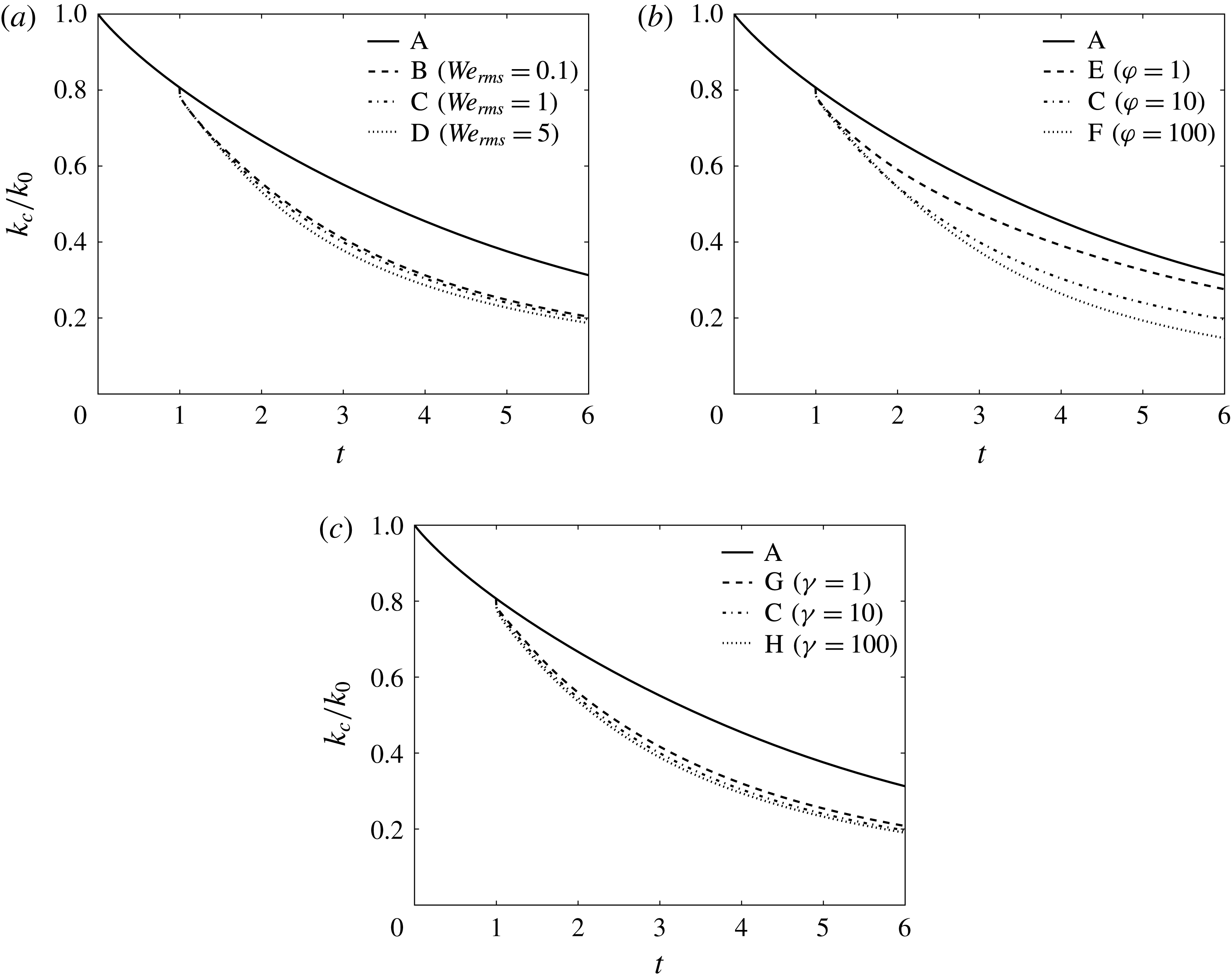
Figure 18 shows the time evolution of the carrier-fluid TKE normalized by its initial value,
 $k_{c}(t)/k_{0}$
, in cases A–H (note that in case A, the droplet-free flow is considered carrier fluid, i.e.
 $k(t)=k_{c}(t)$
). In the droplet-laden cases (B–H),
 $k_{c}(t)$
increases monotonically with decreasing
 $\mathit{We}_{rms}$
,
 $\unicode[STIX]{x1D711}$
or
 $\unicode[STIX]{x1D6FE}$
.
Temporal evolution of the carrier-fluid turbulence kinetic energy,
 $k_{c}$
, normalized by its initial value,
 $k_{0}$
.

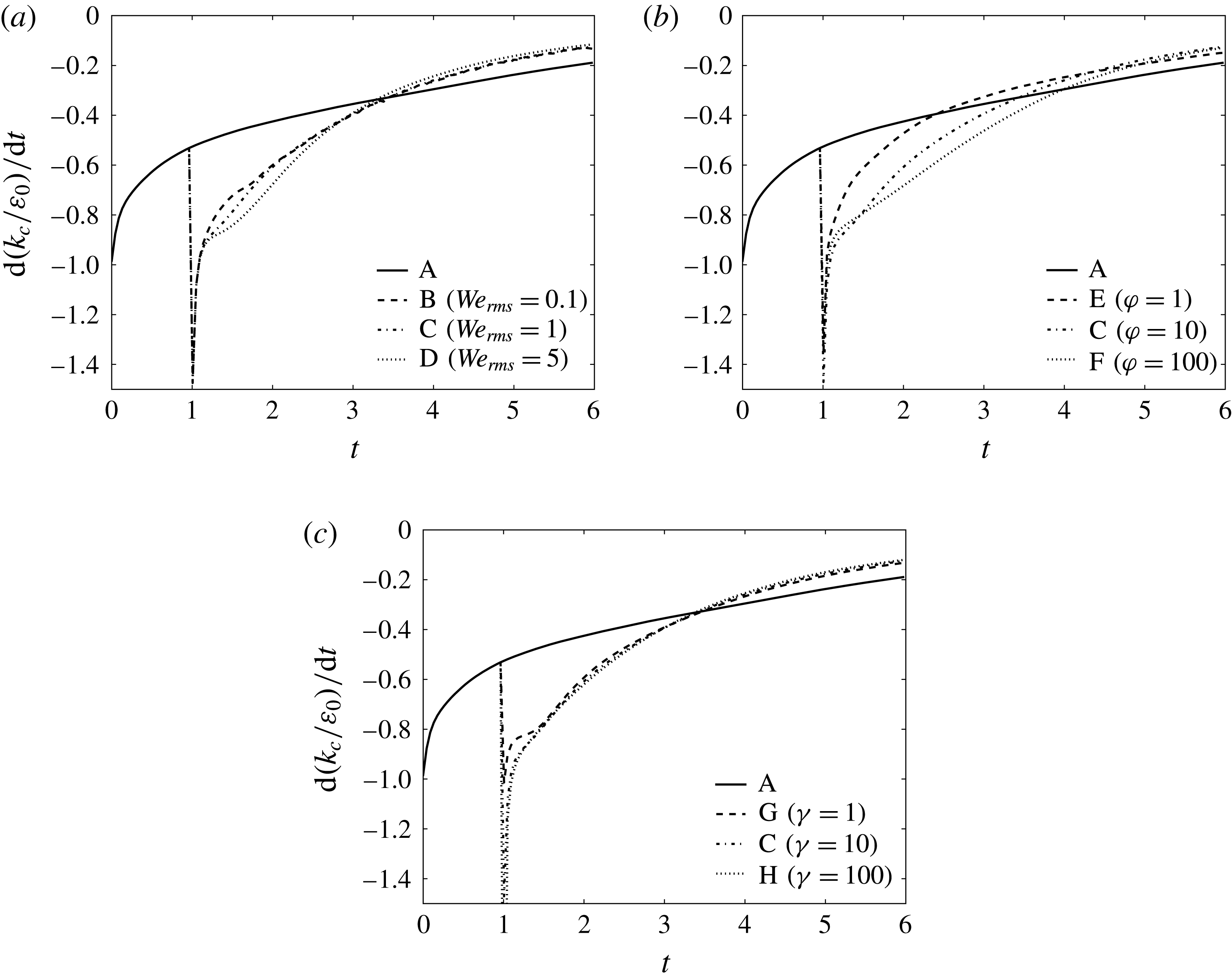
Figure 19 shows the temporal evolution of the rate of change of the carrier-fluid TKE normalized by the initial dissipation rate,
 $\text{d}(k_{c}(t)/\unicode[STIX]{x1D700}_{0})/\text{d}t$
, in cases A–H. For
 $1<t<1+\unicode[STIX]{x1D70F}_{\ell }$
,
 $\text{d}(k_{c}(t)/\unicode[STIX]{x1D700}_{0})/\text{d}t$
increases monotonically for increasing
 $We_{rms}$
(cases B–D), increasing
 $\unicode[STIX]{x1D711}$
(cases E, C and F) or increasing
 $\unicode[STIX]{x1D6FE}$
(cases G, C and H). At later times
 $t>1+\unicode[STIX]{x1D70F}_{\ell }$
, the decay rate of
 $k_{c}(t)$
is nearly independent of
 $We_{rms}$
,
 $\unicode[STIX]{x1D711}$
and
 $\unicode[STIX]{x1D6FE}$
.
Temporal evolution of the rate of change of carrier-fluid turbulence kinetic energy,
 $\text{d}k_{c}(t)/\text{d}t$
, normalized by the initial value of the dissipation rate,
 $\unicode[STIX]{x1D700}_{0}$
.

To explain why the droplets (cases B–H) enhance the decay rate of the carrier-fluid TKE,
 $k_{c}(t)$
, relative to the droplet-free flow (case A), we analyse the time development of the terms on the right-hand side of (3.8):
 $\unicode[STIX]{x1D700}_{c}(t)$
,
 $T_{\unicode[STIX]{x1D708},c}(t)$
and
 $T_{p,c}(t)$
. Figure 20 shows the temporal evolution of the carrier-fluid dissipation rate of TKE normalized by its initial value,
 $\unicode[STIX]{x1D700}_{c}(t)/\unicode[STIX]{x1D700}_{0}$
, in cases A–H.
 $\unicode[STIX]{x1D700}_{c}(t)$
increases when the droplets are released into the flow field (
 $t=1$
). At early times (
 $1<t<1+\unicode[STIX]{x1D70F}_{\ell }$
),
 $\unicode[STIX]{x1D700}_{c}(t)$
is nearly independent of
 $\mathit{We}_{rms}$
(B–D), and it increases with increasing
 $\unicode[STIX]{x1D711}$
(E, C and F) or
 $\unicode[STIX]{x1D6FE}$
(G, C and H). At time
 $t\approx 1+\unicode[STIX]{x1D70F}_{\ell }$
there is a crossover of
 $\unicode[STIX]{x1D700}_{c}(t)$
with case A in all droplet-laden cases B–H. The reason for the crossover is the same as the one explained in § 3.3.1. The time at which the crossover occurs is independent of
 $\mathit{We}_{rms}$
and
 $\unicode[STIX]{x1D6FE}$
, but increases with increasing
 $\unicode[STIX]{x1D711}$
.
Temporal evolution of the carrier-fluid dissipation rate of turbulence kinetic energy,
 $\unicode[STIX]{x1D700}_{c}(t)$
, normalized by its initial value,
 $\unicode[STIX]{x1D700}_{0}$
.

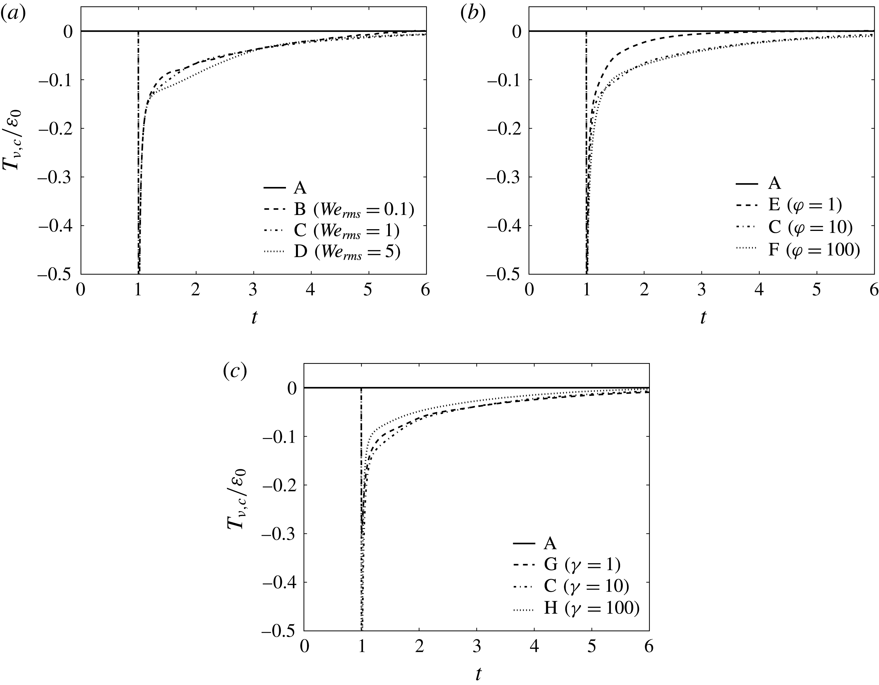
Figure 21 shows the temporal evolution of the normalized power of the viscous stress of the carrier fluid,
 $T_{\unicode[STIX]{x1D708},c}(t)/\unicode[STIX]{x1D700}_{0}$
, in cases A–H. In case A,
 $T_{\unicode[STIX]{x1D708},c}(t)$
is zero because, in spatially homogeneous turbulence, mean quantities (e.g.
 $\langle \unicode[STIX]{x1D61B}_{ij}u_{j}\rangle$
in (3.10)) are invariant with position by definition, and therefore,
 $\unicode[STIX]{x2202}\langle \unicode[STIX]{x1D61B}_{ij}u_{j}\rangle /\unicode[STIX]{x2202}x_{i}=0$
. In contrast, figure 21 shows that in the droplet-laden cases (B–H),
 $T_{\unicode[STIX]{x1D708},c}(t)$
spikes at
 $t=1$
and is negative (a sink of TKE), and then decays, having a magnitude that is roughly 10 % of the initial dissipation rate for
 $1<t<1+\unicode[STIX]{x1D70F}_{\ell }$
.
 $T_{\unicode[STIX]{x1D708},c}(t)$
decreases monotonically in time, while asymptotically approaching zero. Figure 21 also shows that for
 $1<t<1+\unicode[STIX]{x1D70F}_{\ell }$
,
 $T_{\unicode[STIX]{x1D708},c}(t)$
increases for increasing
 $\mathit{We}_{rms}$
and is non-monotonic for varying
 $\unicode[STIX]{x1D711}$
and
 $\unicode[STIX]{x1D6FE}$
. In the cases of varying
 $\unicode[STIX]{x1D711}$
(figure 21
b),
 $T_{\unicode[STIX]{x1D708},c}(t)$
is roughly equivalent for
 $\unicode[STIX]{x1D711}=10$
(case C) and
 $\unicode[STIX]{x1D711}=100$
(case F), and its value is always greater than that for
 $\unicode[STIX]{x1D711}=1$
(case E). Also, figure 21(c) shows that
 $T_{\unicode[STIX]{x1D708},c}(t)$
is roughly equivalent for
 $\unicode[STIX]{x1D6FE}=1$
(case G) and
 $\unicode[STIX]{x1D6FE}=10$
(case C), and its value is always greater than that for
 $\unicode[STIX]{x1D6FE}=100$
(case H).
Temporal evolution of the carrier-fluid viscous power,
 $T_{\unicode[STIX]{x1D708},c}(t)$
, normalized by the initial value of the dissipation rate,
 $\unicode[STIX]{x1D700}_{0}$
.

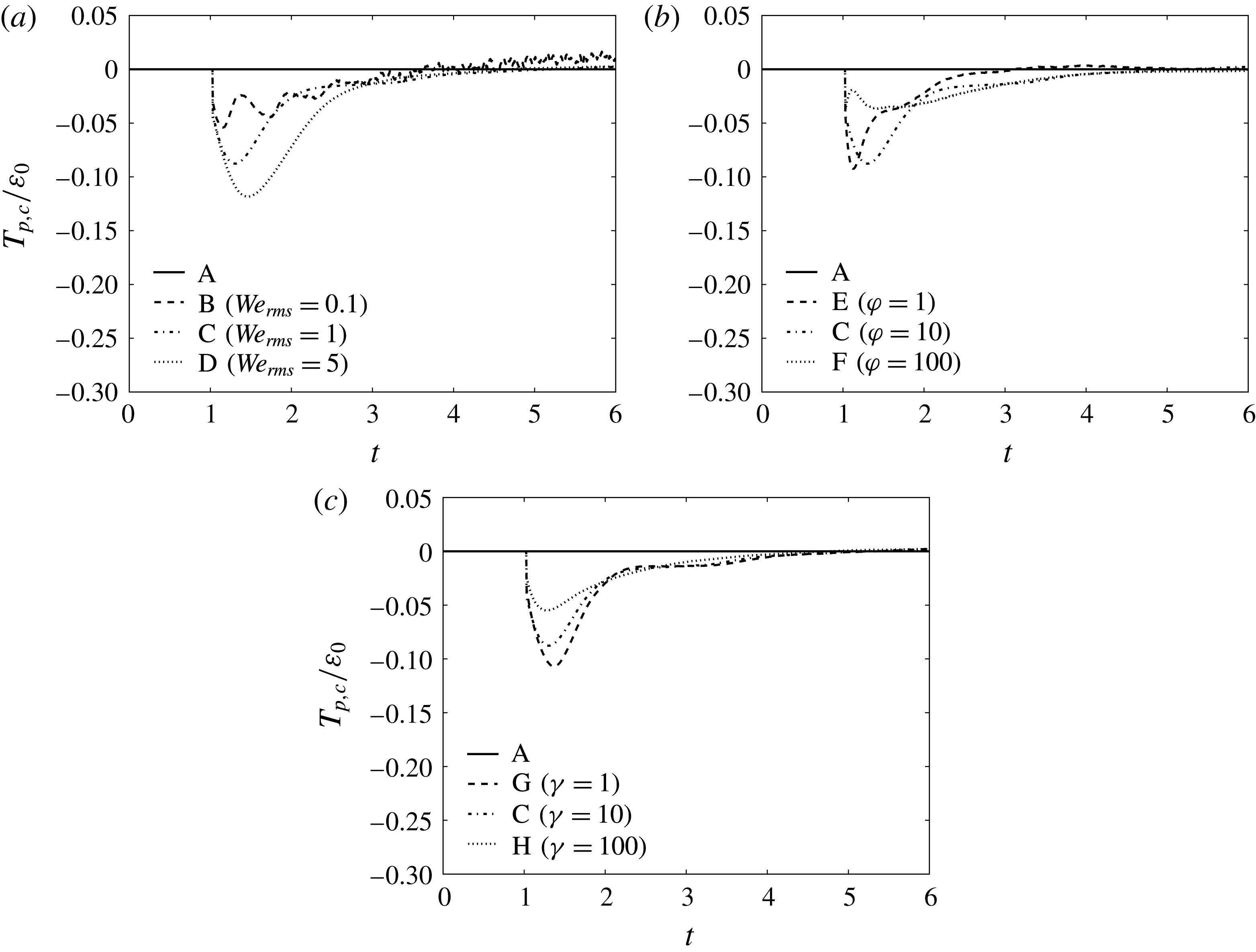
Figure 22 shows that the temporal evolution of the carrier-fluid pressure power,
 $T_{p,c}(t)$
, normalized by
 $\unicode[STIX]{x1D700}_{0}$
in cases A–D. In case A,
 $T_{p,c}(t)$
is zero, as expected for single-phase homogeneous turbulence. In contrast, in cases B–H,
 $T_{p,c}(t)$
is primarily negative; consequently, it is a sink of
 $k_{c}(t)$
. For short times after droplet release (
 $1<t<1+\unicode[STIX]{x1D70F}_{\ell }$
), the pressure power acts as a sink of carrier-fluid TKE with its initial magnitude being approximately 10 % of
 $\unicode[STIX]{x1D700}_{0}$
. As the turbulence decays,
 $T_{p,c}(t)$
decreases in magnitude towards zero. Figure 22 shows that for
 $1<t<2$
,
 $T_{p,c}(t)$
increases monotonically in magnitude for increasing
 $\mathit{We}_{rms}$
or decreasing
 $\unicode[STIX]{x1D6FE}$
, and that the behaviour is non-monotonic for increasing
 $\unicode[STIX]{x1D711}$
.
 $T_{p,c}(t)$
decays more slowly for higher
 $\unicode[STIX]{x1D711}$
, which leads to
 $T_{p,c}(t)$
of the lowest inertia droplets (cases E and C) crossing over that of the highest inertia droplets (case F).
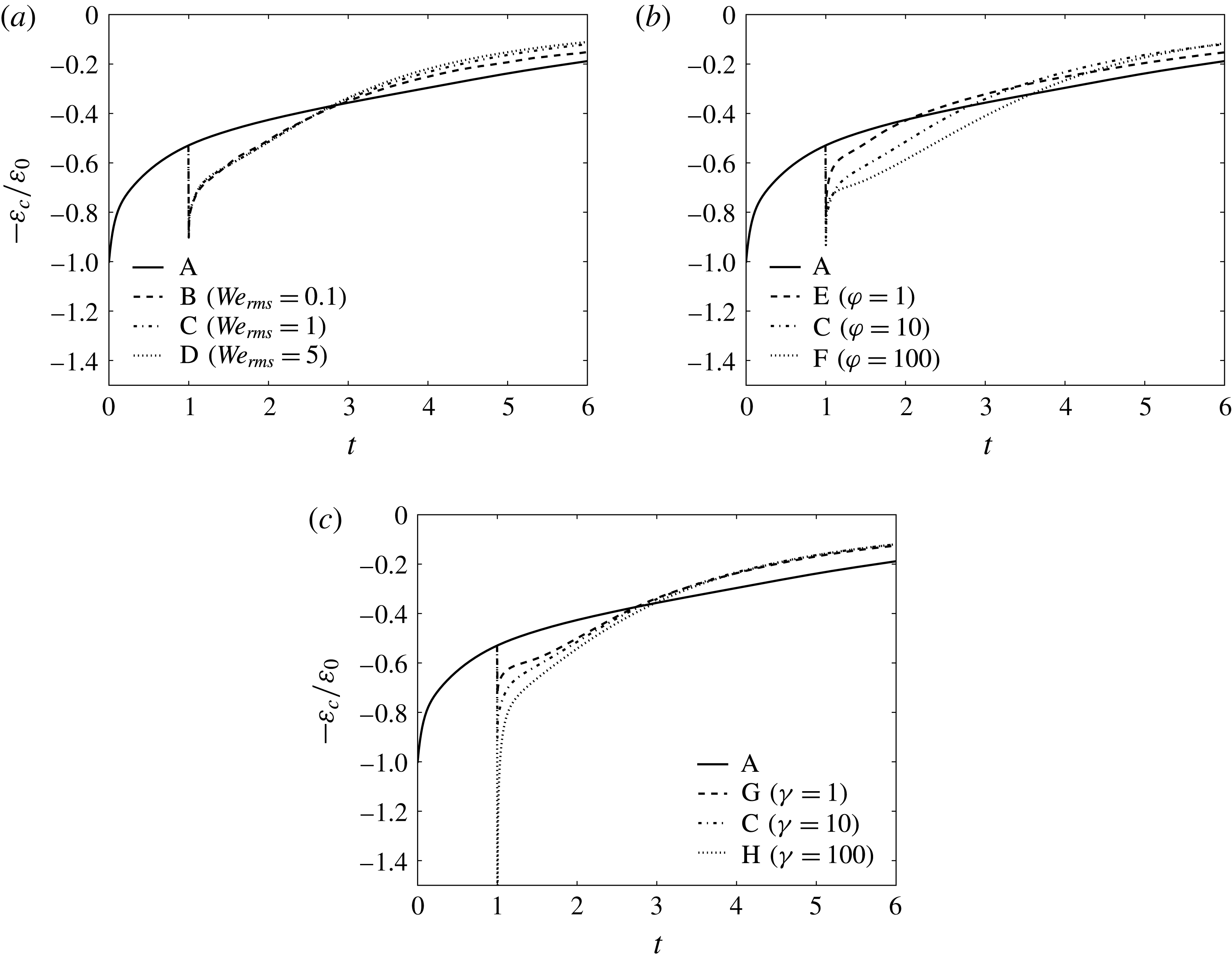
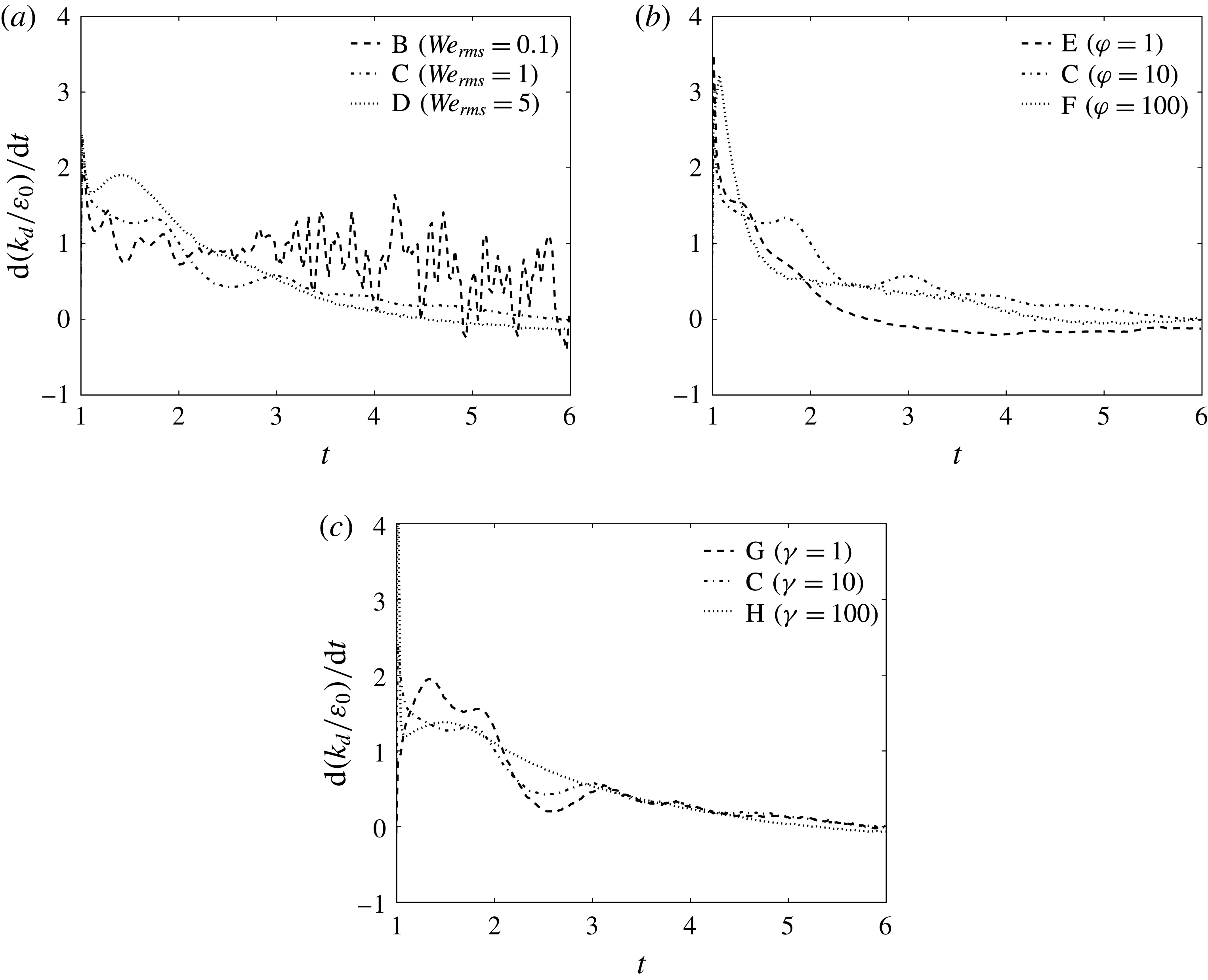
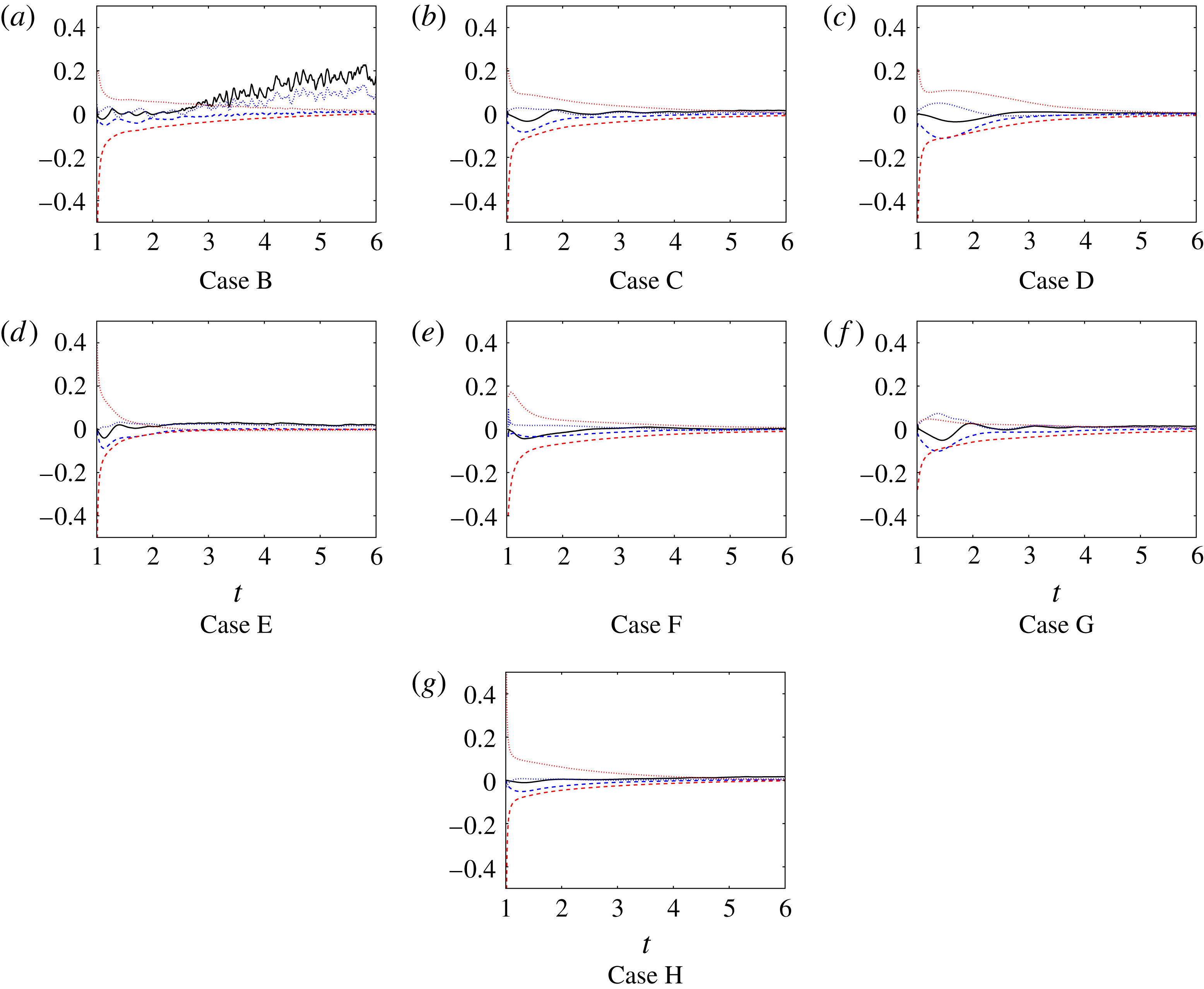
Temporal evolution of the carrier-fluid pressure power,
 $T_{p,c}(t)$
, normalized by the initial value of the dissipation rate,
 $\unicode[STIX]{x1D700}_{0}$
.

The results show that for early times,
 $1<t<1+\unicode[STIX]{x1D70F}_{\ell }$
, the droplets enhance the decay rate of carrier-fluid TKE,
 $\text{d}k_{c}(t)/\text{d}t$
(figure 18), relative to the droplet-free flow. The increased decay rate is due to enhanced dissipation,
 $\unicode[STIX]{x1D700}_{c}(t)$
(figure 20), as well as the presence of viscous power,
 $T_{\unicode[STIX]{x1D708},c}(t)$
, and pressure power,
 $T_{p,c}(t)$
, both of which are sinks of
 $k_{c}(t)$
, as shown in figures 21 and 22, respectively. Most of the carrier-fluid TKE budget
 $\text{d}k_{c}(t)/\text{d}t$
is due to
 $\unicode[STIX]{x1D700}_{c}(t)$
, which makes up roughly 75 % of the budget at
 $t=1$
, and increases to roughly 90 % of the budget at
 $t=6$
. The remainder of the budget (approximately 25 % at
 $t=1$
and 10 % at
 $t=6$
) is split between
 $T_{p,c}(t)$
and
 $T_{\unicode[STIX]{x1D708},c}(t)$
, which have the same order of magnitude.
The increase in
 $\text{d}k_{c}(t)/\text{d}t$
for increasing
 $\mathit{We}_{rms}$
(figure 19
a) is primarily due to increasing pressure power (
 $T_{p,c}(t)$
), and secondarily to increasing viscous power (
 $T_{\unicode[STIX]{x1D708},c}(t)$
). The increase in
 $\text{d}k_{c}(t)/\text{d}t$
for increasing
 $\unicode[STIX]{x1D711}$
and
 $\unicode[STIX]{x1D6FE}$
is due primarily to enhanced
 $\unicode[STIX]{x1D700}_{c}(t)$
.
3.4.2 Droplet-fluid TKE budget
Figure 23 shows the time evolution of the droplet-fluid TKE normalized by its initial value,
 $k_{d}(t)/k_{0}$
in cases B–H. In all cases,
 $k_{d}(t)$
is initially zero because the droplets are released from rest, and then
 $k_{d}(t)$
increases. For
 $1<t<2.5$
,
 $k_{d}(t)$
increases monotonically with increasing Weber number, but for longer times the behaviour is non-monotonic. Figure 23(b) shows that
 $k_{d}(t)$
is non-monotonic for increasing
 $\unicode[STIX]{x1D711}$
, with
 $k_{d}(t)$
increasing when
 $\unicode[STIX]{x1D711}$
increases from 1 to 10, but then decreasing when
 $\unicode[STIX]{x1D711}$
increases to 100. Figure 23(c) shows that
 $k_{d}(t)$
is nearly independent of the viscosity ratio (
 $\unicode[STIX]{x1D6FE}$
).
Temporal evolution of the droplet-fluid turbulence kinetic energy,
 $k_{d}(t)$
, normalized by its initial value,
 $k_{0}$
.

Figure 24 shows the normalized rate of change of the droplet-fluid TKE,
 $\text{d}k_{d}(t)/\text{d}t$
as a function of time. In all droplet-laden cases (B–H),
 $\text{d}k_{d}(t)/\text{d}t$
is initially positive, and then decays in time. For early times
 $1<t<1+\unicode[STIX]{x1D70F}_{\ell }$
,
 $\text{d}k_{d}(t)/\text{d}t$
tends to oscillate, and for later times
 $t>1+\unicode[STIX]{x1D70F}_{\ell }$
,
 $\text{d}k_{d}(t)/\text{d}t$
exhibits fluctuations, especially in case B.
 $\text{d}k_{d}(t)/\text{d}t$
is non-monotonic for varying
 $\mathit{We}_{rms}$
,
 $\unicode[STIX]{x1D711}$
and
 $\unicode[STIX]{x1D6FE}$
.
Temporal evolution of the rate of change of droplet-fluid turbulence kinetic energy,
 $\text{d}k_{d}(t)/\text{d}t$
, normalized by the initial value of the dissipation rate,
 $\unicode[STIX]{x1D700}_{0}$
.

To explain the behaviour of the droplet-fluid TKE decay rate,
 $\text{d}k_{d}(t)/\text{d}t$
, we analyse the time development of the terms on the right-hand side of (3.9):
 $\unicode[STIX]{x1D700}_{d}(t)$
,
 $T_{\unicode[STIX]{x1D708},d}(t)$
and
 $T_{p,d}(t)$
. Figure 25 shows the time evolution of the normalized droplet-fluid dissipation rate of TKE,
 $\unicode[STIX]{x1D700}_{d}(t)/\unicode[STIX]{x1D700}_{0}$
. In all droplet-laden cases (B–H),
 $\unicode[STIX]{x1D700}_{d}(t)/\unicode[STIX]{x1D700}_{0}$
spikes when the droplets are released (
 $t=1$
). For
 $1<t<2.5$
,
 $\unicode[STIX]{x1D700}_{d}(t)$
increases monotonically with increasing
 $\mathit{We}_{rms}$
, increasing
 $\unicode[STIX]{x1D711}$
or decreasing
 $\unicode[STIX]{x1D6FE}$
.
 $\unicode[STIX]{x1D700}_{d}(t)$
tends to decay towards zero, except for in case B, where it grows for later times (
 $t>1+\unicode[STIX]{x1D70F}_{\ell }$
), and, by
 $t=6$
, is roughly ten times greater than that in the other six cases (figure 25
a).
Temporal evolution of the droplet-fluid dissipation rate of turbulence kinetic energy,
 $\unicode[STIX]{x1D700}_{d}(t)$
, normalized by the initial value of the dissipation rate,
 $\unicode[STIX]{x1D700}_{0}$
.

Figure 26 shows the temporal evolution of the normalized, droplet-fluid viscous power,
 $T_{\unicode[STIX]{x1D708},d}(t)/\unicode[STIX]{x1D700}_{0}$
. In all droplet-laden cases (B–H), right after droplet release,
 $T_{\unicode[STIX]{x1D708},d}(t)>0$
, indicating that the viscous power is a source of TKE for the droplets. The magnitude of
 $T_{\unicode[STIX]{x1D708},d}(t)$
decays in time and remains positive, except in case E (
 $\unicode[STIX]{x1D711}=1$
, lowest inertia droplets studied). For
 $1<t<2$
, as
 $\mathit{We}_{rms}$
increases,
 $T_{\unicode[STIX]{x1D708},d}(t)$
increases. The behaviour of
 $T_{\unicode[STIX]{x1D708},d}(t)$
with varying
 $\unicode[STIX]{x1D711}$
and
 $\unicode[STIX]{x1D6FE}$
is non-monotonic.
Temporal evolution of the droplet-fluid viscous power,
 $T_{\unicode[STIX]{x1D708},d}(t)$
, normalized by the initial value of the dissipation rate,
 $\unicode[STIX]{x1D700}_{0}$
.

Figure 27 shows the temporal evolution of the normalized, droplet-fluid pressure power,
 $T_{p,d}(t)/\unicode[STIX]{x1D700}_{0}$
. In cases B–H, right after droplet release,
 $T_{p,d}(t)>0$
, indicating that
 $T_{p,d}(t)$
is a source of TKE for the droplets. For early times (
 $1<t<2.5$
),
 $T_{p,d}(t)$
tends to oscillate, and it may oscillate between positive or negative values as in case B. This indicates that
 $T_{p,d}(t)$
can be a source or sink of TKE in these cases. However,
 $T_{p,d}(t)$
is mostly a source of
 $k_{d}(t)$
. For
 $1<t<2$
,
 $T_{p,d}(t)$
increases for increasing
 $\mathit{We}_{rms}$
or decreasing
 $\unicode[STIX]{x1D6FE}$
. For longer times (
 $t>1+\unicode[STIX]{x1D70F}_{\ell }$
),
 $T_{p,d}(t)$
increases for decreasing
 $\mathit{We}_{rms}$
or decreasing
 $\unicode[STIX]{x1D711}$
.
Temporal evolution of the droplet-fluid pressure power,
 $T_{p,d}$
, normalized by the initial value of the dissipation rate,
 $\unicode[STIX]{x1D700}_{0}$
.

To summarize, for
 $1<t<2$
,
 $k_{d}(t)$
grows in time because
 $T_{\unicode[STIX]{x1D708},d}(t)$
and
 $T_{p,d}(t)$
are both sources of
 $k_{d}(t)$
, and their sum is greater than the droplet-fluid dissipation rate (
 $\unicode[STIX]{x1D700}_{d}(t)$
), and therefore, via (3.9),
 $\text{d}k_{d}(t)/\text{d}t>0$
. For
 $t>1+\unicode[STIX]{x1D70F}_{\ell }$
, the decay in
 $\text{d}k_{d}(t)/\text{d}t$
is caused by
 $T_{\unicode[STIX]{x1D708},d}(t)+T_{p,d}(t)$
decaying more quickly than
 $\unicode[STIX]{x1D700}_{d}(t)$
; consequently,
 $-\unicode[STIX]{x1D700}_{d}(t)+T_{\unicode[STIX]{x1D708},d}(t)+T_{p,d}(t)$
approaches zero, and even becomes negative in cases D, E, F and H. Case B is an exception to this trend, as figure 23(a) shows
 $k_{d}(t)$
continues to grow, which is due to enhanced
 $T_{p,d}(t)$
(figure 27
a) relative to the other six cases. Finally, the oscillations in
 $\text{d}k_{d}(t)/\text{d}t$
(figure 24) are caused by oscillations in
 $T_{p,d}(t)$
(figure 27).
3.4.3 Interfacial energy balance
In figure 5, we have shown that
 $k_{c}(t)$
can be transferred to the droplet fluid (green arrow) or to the interface (blue arrow). This raises the question: how much of
 $k_{c}(t)$
is transferred to
 $k_{d}(t)$
and how much is transferred to
 $\unicode[STIX]{x1D6F9}_{\unicode[STIX]{x1D70E}}(t)$
? Using (3.12), we quantify how much of
 $k_{c}(t)$
goes into
 $k_{d}(t)$
and how much goes into
 $\unicode[STIX]{x1D6F9}_{\unicode[STIX]{x1D70E}}(t)$
. Figure 28 shows the time evolution of the terms in (3.12) in cases B–H. In all cases
 $\unicode[STIX]{x1D719}_{v}(T_{\unicode[STIX]{x1D708},d}(t)+T_{p,d}(t))>\unicode[STIX]{x1D6F9}_{\unicode[STIX]{x1D70E}}(t)$
, indicating that of the
 $k_{c}(t)$
lost via
 $T_{\unicode[STIX]{x1D708},c}(t)+T_{p,c}(t)$
,
 $k_{d}(t)$
gains more of that energy than the interface. Also, figure 28 shows that, in the majority of cases,
 $(1-\unicode[STIX]{x1D719}_{v})T_{p,c}(t)+\unicode[STIX]{x1D719}_{v}T_{p,d}(t)$
is greater than
 $(1-\unicode[STIX]{x1D719}_{v})T_{\unicode[STIX]{x1D708},c}(t)+\unicode[STIX]{x1D719}_{v}T_{\unicode[STIX]{x1D708},d}(t)$
. Therefore, of the
 $k_{c}(t)$
that gets converted to surface energy via
 $\unicode[STIX]{x1D6F9}_{\unicode[STIX]{x1D70E}}(t)$
, most of it comes from
 $T_{p,c}(t)$
.
Time evolution of the normalized terms in the interfacial energy balance equation (3.12),
 $\unicode[STIX]{x1D6F9}_{\unicode[STIX]{x1D70E}}(t)=(1-\unicode[STIX]{x1D719}_{v})[T_{\unicode[STIX]{x1D708},c}(t)+T_{p,c}(t)]+\unicode[STIX]{x1D719}_{v}[T_{\unicode[STIX]{x1D708},d}(t)+T_{p,d}(t)]$
in cases B–H.
 $\unicode[STIX]{x1D6F9}_{\unicode[STIX]{x1D70E}}/\unicode[STIX]{x1D700}_{0}$
(solid black line);
 $(1-\unicode[STIX]{x1D719}_{v})T_{p,c}/\unicode[STIX]{x1D700}_{0}$
(dashed blue line);
 $(1-\unicode[STIX]{x1D719}_{v})T_{\unicode[STIX]{x1D708},c}/\unicode[STIX]{x1D700}_{0}$
(dashed red line);
 $\unicode[STIX]{x1D719}_{v}T_{p,d}/\unicode[STIX]{x1D700}_{0}$
(dotted blue line);
 $\unicode[STIX]{x1D719}_{v}T_{\unicode[STIX]{x1D708},d}/\unicode[STIX]{x1D700}_{0}$
(dotted red line).

3.4.4 Dissipation rate of TKE in the carrier and droplet fluid
In § 3.4.1, the results showed that
 $\unicode[STIX]{x1D700}_{c}(t)$
increases for increasing density ratio,
 $\unicode[STIX]{x1D711}$
(figure 20
b) and, in § 3.4.2, the same trend was shown for
 $\unicode[STIX]{x1D700}_{d}(t)$
. We now explain why
 $\unicode[STIX]{x1D700}_{c}(t)$
and
 $\unicode[STIX]{x1D700}_{d}(t)$
increase with
 $\unicode[STIX]{x1D711}$
. Figure 12 shows that as
 $\unicode[STIX]{x1D711}$
increases (cases E and F),
 $\unicode[STIX]{x1D700}^{\prime }$
increases at the carrier- and droplet-fluid side of the interface (the physical mechanism for the increase is explained in § 3.3.2). The local increase of
 $\unicode[STIX]{x1D700}^{\prime }$
in the carrier and droplet fluid increases both
 $\unicode[STIX]{x1D700}_{c}(t)$
and
 $\unicode[STIX]{x1D700}_{d}(t)$
because
 $\unicode[STIX]{x1D700}_{c}(t)=\langle \unicode[STIX]{x1D700}^{\prime }\rangle _{c}$
and
 $\unicode[STIX]{x1D700}_{d}(t)=\langle \unicode[STIX]{x1D700}^{\prime }\rangle _{d}$
, respectively.
It was also shown in § 3.4.1 that, for increasing viscosity ratio,
 $\unicode[STIX]{x1D6FE}$
,
 $\unicode[STIX]{x1D700}_{c}(t)$
increases (figure 20
c) and
 $\unicode[STIX]{x1D700}_{d}(t)$
decreases (figure 25
c). To explain this behaviour, we analyse how varying
 $\unicode[STIX]{x1D6FE}$
modulates the velocity field at the droplet interface. Figure 29 shows the velocity profiles in an
 $x$
-
 $y$
plane,
 $u(y)$
, through the midsection of a droplet in cases G (
 $\unicode[STIX]{x1D6FE}=1$
) and H (
 $\unicode[STIX]{x1D6FE}=100$
). The figure shows that (i)
 $\unicode[STIX]{x2202}u/\unicode[STIX]{x2202}y$
at the interface is continuous for
 $\unicode[STIX]{x1D6FE}=1$
and discontinuous for
 $\unicode[STIX]{x1D6FE}=100$
and (ii) the magnitude of the velocity gradient in the carrier fluid (
 $\unicode[STIX]{x2202}u_{c}/\unicode[STIX]{x2202}y$
) increases as
 $\unicode[STIX]{x1D6FE}$
increases from 1 to 100. To explain this, consider two cases of the flow near the interface of a droplet initially released from rest in two uniform flows with the same
 $\mathit{Re}$
,
 $\mathit{We}_{rms}$
and
 $\unicode[STIX]{x1D711}$
, but different
 $\unicode[STIX]{x1D6FE}$
(figure 30). The boundary conditions at the droplet interface (appendix A) stipulate that: (i) the velocity is continuous
 $$\begin{eqnarray}u_{c}=u_{d},\end{eqnarray}$$
and (ii) the tangential stress is continuous
 $$\begin{eqnarray}\unicode[STIX]{x1D707}_{c}\frac{\unicode[STIX]{x2202}u_{c}}{\unicode[STIX]{x2202}y}=\unicode[STIX]{x1D707}_{d}\frac{\unicode[STIX]{x2202}u_{d}}{\unicode[STIX]{x2202}y}\rightarrow \frac{\unicode[STIX]{x2202}u_{c}}{\unicode[STIX]{x2202}y}=\unicode[STIX]{x1D6FE}\frac{\unicode[STIX]{x2202}u_{d}}{\unicode[STIX]{x2202}y}.\end{eqnarray}$$
Figure 30 shows that as
 $\unicode[STIX]{x1D6FE}$
increases,
 $\unicode[STIX]{x2202}u_{c}/\unicode[STIX]{x2202}y$
increases and
 $\unicode[STIX]{x2202}u_{d}/\unicode[STIX]{x2202}y$
decreases near the interface, consequently, because
 $\unicode[STIX]{x1D700}^{\prime }$
is proportional to
 $\unicode[STIX]{x1D707}(\unicode[STIX]{x2202}u/\unicode[STIX]{x2202}y)^{2}$
,
 $\unicode[STIX]{x1D700}^{\prime }$
near the interface increases in the carrier fluid and decreases in the droplet fluid. This mechanism can also be seen in droplet-laden isotropic turbulence by comparing contours of
 $\unicode[STIX]{x1D700}^{\prime }$
in cases G (
 $\unicode[STIX]{x1D6FE}=1$
) and H (
 $\unicode[STIX]{x1D6FE}=100$
), which are shown in figure 31 at
 $t=1.5$
and supplementary movie 5.
Cross sections of a droplet (black line;
 $C=0.5$
isoline) showing the
 $u$
-velocity profile,
 $u(y)$
, (blue line) taken at the dashed line in cases G (a,c) and H (b,d) at
 $t=1.2$
(a,b) and
 $t=2$
(c,d). Contrasting
 $u(y)$
in both figures, we see that
 $\unicode[STIX]{x2202}u/\unicode[STIX]{x2202}y$
is discontinuous in case H (
 $\unicode[STIX]{x1D6FE}=100$
) and that
 $\unicode[STIX]{x2202}u/\unicode[STIX]{x2202}y$
in the carrier fluid is greater in case H than it is in case G.

Illustration of the velocity profile,
 $u(y)$
, at the interface of a droplet released from rest in uniform flow. The illustration depicts the effects of varying the viscosity ratio,
 $\unicode[STIX]{x1D6FE}$
. Unity viscosity ratio
 $\unicode[STIX]{x1D6FE}=1$
(a); viscosity ratio greater than unity
 $\unicode[STIX]{x1D6FE}>1$
(b).

Instantaneous contours in a subregion of the
 $x{-}z$
plane of
 $\unicode[STIX]{x1D700}^{\prime }=\mathit{Re}^{-1}(\unicode[STIX]{x1D61B}_{ij}\unicode[STIX]{x1D61A}_{ij})$
in (a) case G and (b) case H at
 $t=1.5$
.

3.4.5 Viscous power
In §§ 3.4.1 and 3.4.2, the results have shown that the viscous power is a sink of TKE for the carrier fluid (
 $T_{\unicode[STIX]{x1D708},c}(t)<0$
) and a source of TKE for the droplet fluid (
 $T_{\unicode[STIX]{x1D708},d}(t)>0$
). We now explain why
 $T_{\unicode[STIX]{x1D708},c}(t)<0$
and
 $T_{\unicode[STIX]{x1D708},d}(t)>0$
and how varying
 $\mathit{We}_{rms}$
,
 $\unicode[STIX]{x1D711}$
and
 $\unicode[STIX]{x1D6FE}$
changes their magnitude.
Figure 32 shows the instantaneous two-dimensional contours of
 $T_{\unicode[STIX]{x1D708}}^{\prime }\equiv \mathit{Re}^{-1}\unicode[STIX]{x2202}(\unicode[STIX]{x1D61B}_{ij}u_{j})/\unicode[STIX]{x2202}x_{i}$
in a subregion of the computational domain at
 $t=1.1$
(supplementary movie 6 shows the animated contours for
 $1<t<3.5$
). For single-phase flow
 $T_{\unicode[STIX]{x1D708},c}(t)=0$
, figure 32(a) shows regions of
 $T_{\unicode[STIX]{x1D708}}^{\prime }>0$
and
 ${<}0$
. In contrast, in the droplet-laden flow (case C), figure 32(b) shows that
 $T_{\unicode[STIX]{x1D708}}^{\prime }$
is preferentially negative in the carrier fluid and positive in the droplet fluid. Such modulation of
 $T_{\unicode[STIX]{x1D708}}^{\prime }$
by the droplets induces
 $T_{\unicode[STIX]{x1D708},c}(t)<0$
and
 $T_{\unicode[STIX]{x1D708},d}(t)>0$
because
 $T_{\unicode[STIX]{x1D708},c}(t)=\langle T_{\unicode[STIX]{x1D708}}^{\prime }\rangle _{c}$
and
 $T_{\unicode[STIX]{x1D708},d}(t)=\langle T_{\unicode[STIX]{x1D708}}^{\prime }\rangle _{d}$
. Finally,
 $T_{\unicode[STIX]{x1D708},c}(t)<0$
and
 $T_{\unicode[STIX]{x1D708},d}(t)>0$
indicates that there is a net flux of TKE from the carrier fluid to the droplet fluid.
Instantaneous contours in a subregion of the
 $x{-}z$
plane of
 $T_{\unicode[STIX]{x1D708}}^{\prime }=\mathit{Re}^{-1}\unicode[STIX]{x2202}(u_{j}\unicode[STIX]{x1D61B}_{ij})/\unicode[STIX]{x2202}x_{i}$
in (a) case A and (b) case C at
 $t=1.1$
.

In § 3.4.1, the results showed that, for early times
 $1<t<1+\unicode[STIX]{x1D70F}_{\ell }$
,
 $T_{\unicode[STIX]{x1D708},c}(t)$
increases in magnitude with increasing Weber number. The reason for the behaviour is unclear from analysing two-dimensional contours of
 $T_{\unicode[STIX]{x1D708}}^{\prime }$
in cases B and D (not shown), because they are qualitatively similar. Therefore, to explain the behaviour, we begin be rewriting
 $T_{\unicode[STIX]{x1D708},c}(t)$
(3.10) as a volume integral, and then by transforming it to a surface integral using the divergence theorem as
 $$\begin{eqnarray}T_{\unicode[STIX]{x1D708},c}(t)=\frac{1}{\mathscr{V}_{c}}\mathop{\sum }_{n=1}^{N_{d}}\frac{1}{\mathit{Re}}\iint _{\unicode[STIX]{x2202}\mathscr{V}_{c}^{(n)}(t)}(\unicode[STIX]{x1D64F}\boldsymbol{u}\boldsymbol{\cdot }\boldsymbol{n})\,\text{d}\mathscr{A}.\end{eqnarray}$$
Equation (3.20) can be interpreted as the rate of work on the carrier fluid due to the viscous stress acting on
 $\unicode[STIX]{x2202}\mathscr{V}_{c}^{(n)}$
. We note that the contributions from the boundaries of the computational domain sum to zero due to periodicity, and therefore, the power in (3.20) is due entirely to viscous forces exerted on the carrier fluid by the droplets. Therefore,
 $T_{\unicode[STIX]{x1D708},c}(t)$
can be interpreted as the work on the carrier fluid due to viscous drag from the droplets.
Equation (3.20) shows that
 $T_{\unicode[STIX]{x1D708},c}(t)$
depends on both the magnitude of the integrand and the amount of droplet surface area over which the integration is performed. This dependence is expressed as
 $$\begin{eqnarray}T_{\unicode[STIX]{x1D708},c}(t)=\frac{1}{\mathscr{V}_{c}}G_{\unicode[STIX]{x1D708}}(t)A(t),\end{eqnarray}$$
where
 $A(t)$
is the instantaneous total surface area of the droplets (3.14) and
 $G_{\unicode[STIX]{x1D708}}(t)$
is the mean value of the integrand in (3.20), which is defined as
 $$\begin{eqnarray}G_{\unicode[STIX]{x1D708}}(t)=\frac{1}{A(t)}\frac{1}{\mathit{Re}}\mathop{\sum }_{n=1}^{N_{d}(t)}\iint _{\unicode[STIX]{x2202}\mathscr{V}_{c}^{(n)}(t)}(|\boldsymbol{u}|\,|\unicode[STIX]{x1D64F}\boldsymbol{n}|\cos (\unicode[STIX]{x1D703}_{\unicode[STIX]{x1D708}}))\,\text{d}\mathscr{A}.\end{eqnarray}$$
Compared to that in (3.20), we have rewritten the integrand in (3.22) in terms of the magnitude of the velocity vector,
 $|\boldsymbol{u}|$
, the magnitude of the traction vector,
 $|\unicode[STIX]{x1D64F}\boldsymbol{n}|$
, and the angle,
 $\unicode[STIX]{x1D703}_{\unicode[STIX]{x1D708}}$
, formed between
 $\boldsymbol{u}$
and
 $\unicode[STIX]{x1D64F}\boldsymbol{n}$
. Table 4 shows the normalized values of
 $G_{\unicode[STIX]{x1D708}}(t)$
and
 $A(t)$
at
 $t=1.5$
.
Droplet surface statistics in the carrier fluid at
 $t=1.5$
. The quantities denoted with the superscript
 $^{\ast }$
are normalized as follows:
 $G_{\unicode[STIX]{x1D708}}$
and
 $G_{p}$
are normalized by
 $1/2\unicode[STIX]{x1D70C}U_{\mathit{rms,1}}^{3}$
,
 $\overline{|\boldsymbol{u}|}$
is normalized by
 $U_{\mathit{rms,1}}$
, and
 $\mathit{Re}^{-1}\overline{|\unicode[STIX]{x1D64F}\boldsymbol{n}|}$
and
 $\overline{|-p\boldsymbol{n}|}$
are normalized by
 $1/2\unicode[STIX]{x1D70C}U_{\mathit{rms,1}}^{2}$
.

Table 4 shows that as
 $\mathit{We}_{rms}$
increases from 0.1 to 5,
 $G_{\unicode[STIX]{x1D708}}(t)$
increases in magnitude by 25 % and
 $A(t)$
increases by 6 %, and therefore, both contribute to an increase in the magnitude of
 $T_{\unicode[STIX]{x1D708},c}(t)$
. To explain the increase in magnitude of
 $G_{\unicode[STIX]{x1D708}}(t)$
, we analyse the ensemble average (
 $\overline{\cdots \,}$
) of the following terms from the right-hand side of (3.22):
 $|\boldsymbol{u}|$
,
 $\mathit{Re}^{-1}|\unicode[STIX]{x1D64F}\boldsymbol{n}|$
, and
 $\cos (\unicode[STIX]{x1D703}_{\unicode[STIX]{x1D708}})$
. Table 4 shows that as
 $\mathit{We}_{rms}$
increases from 0.1 to 5,
 $\overline{\cos (\unicode[STIX]{x1D703}_{\unicode[STIX]{x1D708}})}$
is roughly constant, and thus, it is not responsible for the increase in
 $G_{\unicode[STIX]{x1D708}}(t)$
. Table 4 also shows that as
 $\mathit{We}_{rms}$
increases from 0.1 to 5,
 $\overline{|\boldsymbol{u}|}$
increases by 12 % and
 $\mathit{Re}^{-1}|\unicode[STIX]{x1D64F}\boldsymbol{n}|$
stays nearly constant. Figure 34(a–c) shows the scatter plot of
 $|\boldsymbol{u}|$
and
 $\mathit{Re}^{-1}|\unicode[STIX]{x1D64F}\boldsymbol{n}|$
for 4000 randomly selected samples, and that
 $|\boldsymbol{u}|$
and
 $\mathit{Re}^{-1}|\unicode[STIX]{x1D64F}\boldsymbol{n}|$
are positively correlated. Consequently, as
 $\overline{|\boldsymbol{u}|}$
increases with
 $\mathit{We}_{rms}$
,
 $\mathit{Re}^{-1}\overline{|\boldsymbol{u}||\unicode[STIX]{x1D64F}\boldsymbol{n}|}$
also increases, such as to increase the right-hand side of (3.22), i.e. increases
 $G_{\unicode[STIX]{x1D708}}(t)$
.
To explain the increase in
 $\overline{|\boldsymbol{u}|}$
with increasing
 $\mathit{We}_{rms}$
, we analyse the pressure distribution on the droplet. Flow separation in cases B–D leads to fore-aft asymmetry in the pressure distribution, in which the pressure is higher on the windward side of the droplet than it is on the leeward side, as shown in figure 33. In case B, because
 $\mathit{We}_{rms}=0.1$
, the surface tension forces dominate pressure forces, consequently, the droplets remain spherical. As
 $\mathit{We}_{rms}$
increases to 1 (case C) and 5 (case D), the pressure forces increasingly overcome surface tension forces, leading to droplet deformation. Because the pressure on the windward side of the droplet is greater than that on the leeward side (figure 33), the droplets tend to flatten with the largest dimension perpendicular to the direction of the flow. Such deformation makes the droplet less streamlined and increases the droplet frontal area. The consequences of the deformation can be quantified by computing the pressure force acting on the carrier fluid due to the
 $n$
th droplet as
 $$\begin{eqnarray}\boldsymbol{F}_{p}^{(n)}(t)=\iint _{\unicode[STIX]{x2202}\mathscr{V}_{c}^{(n)}(t)}(-p\boldsymbol{n})\,\text{d}\mathscr{A}.\end{eqnarray}$$
Figure 33 shows
 $\boldsymbol{F}_{p}^{(n)}(t)$
for a selected droplet in cases B and D. Comparing figures 33(a) and (b) reveals that
 $\boldsymbol{F}_{p}(t)$
increases with increasing
 $\mathit{We}_{rms}$
. The force on the droplet is
 $-\boldsymbol{F}_{p}(t)$
, and therefore, as
 $\mathit{We}_{rms}$
increases, the pressure force on the droplet increases, consequently the droplet acceleration increases, and thus the droplet surface velocity
 $|\boldsymbol{u}|$
increases. This is proved by the increase in the size of the tails of the
 $|\boldsymbol{u}|$
distribution (i.e. (
 $|\boldsymbol{u}|>0.6$
)), as shown in figure 34, and by the increase of
 $\overline{|\boldsymbol{u}|}$
with
 $\mathit{We}_{rms}$
, as shown in table 4.
Instantaneous contours of normalized pressure in a subregion of the
 $x{-}z$
plane at
 $t=1.5$
in (a) case B and (b) case D. Small black arrows are fluid velocity vectors projected on the
 $x{-}z$
plane, and the large black arrow is the resultant pressure force acting on the carrier fluid from the droplet,
 $\boldsymbol{F}_{p}$
(3.23). The droplet fluid is masked for clarity.

Scatter plots of
 $|\boldsymbol{u}|$
versus
 $\mathit{Re}^{-1}|\unicode[STIX]{x1D64F}\boldsymbol{n}|$
(a–c) and
 $\cos (\unicode[STIX]{x1D703}_{\unicode[STIX]{x1D708}})$
versus
 $\mathit{Re}^{-1}|\unicode[STIX]{x1D64F}\boldsymbol{n}|$
(d–f) in cases B–D for 4000 randomly selected samples at
 $t=1.5$
. One-dimensional probability density functions of the corresponding variables are shown in the margins of each scatter plot.

In § 3.4.1, figure 21(b) shows that for increasing
 $\unicode[STIX]{x1D711}$
from 1 to 100,
 $T_{\unicode[STIX]{x1D708},c}(t)$
is lowest in magnitude for
 $\unicode[STIX]{x1D711}=1$
(case E), whereas
 $T_{\unicode[STIX]{x1D708},c}(t)$
for
 $\unicode[STIX]{x1D711}=10$
and 100 (cases C and F) was roughly equal. Table 4 shows that, in cases C and F,
 $G_{\unicode[STIX]{x1D708}}(t)$
increases in magnitude by 95 % and 81 %, respectively, with respect to case E. The droplet surface area,
 $A(t)$
, varies by 1 % between the three cases. Therefore, via (3.21), the increase of
 $T_{\unicode[STIX]{x1D708},c}(t)$
in cases C and F relative to case E is primarily due to increasing
 $G_{\unicode[STIX]{x1D708}}(t)$
. To explain the increase in magnitude of
 $G_{\unicode[STIX]{x1D708}}(t)$
, figure 35(d–f) show that when
 $\unicode[STIX]{x1D711}=1$
(case E),
 $\cos \unicode[STIX]{x1D703}_{\unicode[STIX]{x1D708}}$
is nearly uniformly distributed between
 $-1$
and 0.4, whereas when
 $\unicode[STIX]{x1D711}=10$
and 100 (case C and F),
 $\cos \unicode[STIX]{x1D703}_{\unicode[STIX]{x1D708}}$
has values primarily at
 $-1$
. Also, table 4 shows that
 $\overline{\cos (\unicode[STIX]{x1D703}_{\unicode[STIX]{x1D708}})}$
in case E is approximately half of that in cases C and F. At the same time, table 4 shows that as
 $\unicode[STIX]{x1D711}$
increases,
 $\overline{|\boldsymbol{u}|}$
decreases,
 $\mathit{Re}^{-1}\overline{|\boldsymbol{u}||\unicode[STIX]{x1D64F}\boldsymbol{n}|}$
increases and
 $\overline{\cos (\unicode[STIX]{x1D703}_{\unicode[STIX]{x1D708}})}$
increases. Figure 35(a–c) shows that the increase in
 $\overline{|\boldsymbol{u}||\unicode[STIX]{x1D64F}\boldsymbol{n}|}$
is balanced by the decrease in
 $\overline{|\boldsymbol{u}|}$
, and thus, the increase in
 $\overline{\cos (\unicode[STIX]{x1D703}_{\unicode[STIX]{x1D708}})}$
from case E to C is responsible for the increase in the magnitude of
 $G_{\unicode[STIX]{x1D708}}(t)$
, and therefore,
 $T_{\unicode[STIX]{x1D708},c}(t)$
. Furthermore, the increase in
 $\cos \unicode[STIX]{x1D703}_{\unicode[STIX]{x1D708}}$
with increasing
 $\unicode[STIX]{x1D711}$
is explained as follows. We recall from § 3.3.2 that as
 $\unicode[STIX]{x1D711}$
increases the droplet inertia increases, leading to the droplet trajectories deviating more from the surrounding fluid trajectories. As a consequence, as
 $\unicode[STIX]{x1D711}$
increases, the viscous force on the carrier fluid,
 $\unicode[STIX]{x1D64F}\boldsymbol{n}$
, becomes increasingly misaligned with the local velocity
 $\boldsymbol{u}$
, thus increasing
 $\unicode[STIX]{x1D703}_{\unicode[STIX]{x1D708}}$
.
Scatter plots of
 $|\boldsymbol{u}|$
versus
 $\mathit{Re}^{-1}|\unicode[STIX]{x1D64F}\boldsymbol{n}|$
(a–c) and
 $\cos (\unicode[STIX]{x1D703}_{\unicode[STIX]{x1D708}})$
versus
 $\mathit{Re}^{-1}|\unicode[STIX]{x1D64F}\boldsymbol{n}|$
(d–f) in cases E, C and F for 4000 randomly selected samples at
 $t=1.5$
. One-dimensional probability density functions of the corresponding variables are shown in the margins of each scatter plot.

Finally, we analyse in more detail the effects of
 $\unicode[STIX]{x1D6FE}$
on
 $T_{\unicode[STIX]{x1D708},c}(t)$
. Figure 21(c) shows that
 $T_{\unicode[STIX]{x1D708},c}(t)$
is roughly equivalent for
 $\unicode[STIX]{x1D6FE}=1$
(case G) and
 $\unicode[STIX]{x1D6FE}=10$
(case C), and its value is always greater than that for
 $\unicode[STIX]{x1D6FE}=100$
(case H). Table 4 shows that
 $A(t)$
decreases monotonically by 2 % from case G to case F, and that in cases C and G,
 $G_{\unicode[STIX]{x1D708}}(t)$
increases in magnitude by 44 % and 25 %, respectively, with respect to case H. Therefore, via (3.21), the increase of
 $T_{\unicode[STIX]{x1D708},c}(t)$
in cases C and G relative to case H is mainly due to increasing
 $G_{\unicode[STIX]{x1D708}}(t)$
. To explain the increase in magnitude of
 $G_{\unicode[STIX]{x1D708}}(t)$
, table 4 and figure 36(d–f) show that
 $\overline{|\boldsymbol{u}|}$
,
 $\mathit{Re}^{-1}\overline{|\boldsymbol{u}||\unicode[STIX]{x1D64F}\boldsymbol{n}|}$
and
 $\overline{\cos (\unicode[STIX]{x1D703}_{\unicode[STIX]{x1D708}})}$
are higher in cases C and G than they are in case H. Thus, it is the combination of these factors that leads to the increase in
 $G_{\unicode[STIX]{x1D708}}(t)$
from case H to C, and therefore,
 $T_{\unicode[STIX]{x1D708},c}(t)$
. However, among the three terms,
 $\overline{|\boldsymbol{u}|}$
shows the greatest increase in cases C and G relative to case H, with an increase by a factor of 1.7 and 2.6, respectively. The increase in
 $\overline{|\boldsymbol{u}|}$
with decreasing
 $\unicode[STIX]{x1D6FE}$
is explained by figure 30. Note that in the limit
 $\unicode[STIX]{x1D6FE}\rightarrow \infty$
, which corresponds to
 $\unicode[STIX]{x1D707}_{d}\rightarrow \infty$
, momentum diffuses instantaneously in the droplet, and thus, the droplet behaves as a rigid body, whereas in the limit
 $\unicode[STIX]{x1D6FE}\rightarrow 0$
, which corresponds to
 $\unicode[STIX]{x1D707}_{d}\rightarrow 0$
, the droplet surface behaves as a free-shear (slip) boundary.
Scatter plots of
 $|\boldsymbol{u}|$
versus
 $\mathit{Re}^{-1}|\unicode[STIX]{x1D64F}\boldsymbol{n}|$
(a–c) and
 $\cos (\unicode[STIX]{x1D703}_{\unicode[STIX]{x1D708}})$
versus
 $\mathit{Re}^{-1}|\unicode[STIX]{x1D64F}\boldsymbol{n}|$
(d–f) in cases G, C and H for 4000 randomly selected samples at
 $t=1.5$
. One-dimensional probability density functions of the corresponding variables are shown in the margins of each scatter plot.

Table 4 shows that, at
 $t=1.5$
, as
 $\unicode[STIX]{x1D6FE}$
increases from 1 to 100, the mean droplet surface velocity
 $\overline{|\boldsymbol{u}|}$
decreases by 61 %. At the same time, table 5 shows that the mean droplet velocity,
 $\overline{|\boldsymbol{V}_{d}|}$
, increases by a factor of 3.6. Figure 23(c) shows that the decrease in
 $\overline{|\boldsymbol{u}|}$
and the increase in
 $\overline{|\boldsymbol{V}_{d}|}$
balance in such a way that the droplet kinetic energy,
 $k_{d}(t)$
, is nearly independent of
 $\unicode[STIX]{x1D6FE}$
. This suggests that as
 $\unicode[STIX]{x1D6FE}$
increases, the
 $k_{d}(t)$
associated with internal circulation decreases and the
 $k_{d}(t)$
associated with mean droplet translation increases.
Droplet statistics at
 $t=1.5$
in cases B–H.
 $\overline{|\boldsymbol{V}_{d}|}$
is the ensemble average of the mean droplet velocity magnitude and
 $k_{d}(t)$
is the droplet velocity (
 $U_{\mathit{rms,1}}$
and
 $k_{c,1}$
are the r.m.s. velocity and TKE at
 $t=1$
.). Columns 4–6 are the percentage of droplet TKE associated with droplet translation (
 $k_{d,\mathit{trans}}(t)$
), rotation (
 $k_{d,\mathit{rot}}(t)$
), and internal circulation (
 $k_{d,\mathit{int}}(t)$
).

To prove this statement from the DNS data, in appendix D, we decompose
 $k_{d}(t)$
as
 $$\begin{eqnarray}k_{d}(t)=k_{d,\mathit{trans}}(t)+k_{d,\mathit{rot}}(t)+k_{d,\mathit{int}}(t),\end{eqnarray}$$
where
 $k_{d,\mathit{trans}}(t)$
is translational TKE,
 $k_{d,\mathit{rot}}(t)$
is the rotational TKE, and
 $k_{d,\mathit{int}}(t)$
is the TKE associated with internal circulation, and compute the three forms of droplet kinetic energy using the derived formulae of (D 10). Table 5 shows that as
 $\unicode[STIX]{x1D6FE}$
increases (cases G, C and H),
 $k_{d,\mathit{trans}}(t)$
increases from 49 % to 95 %,
 $k_{d,\mathit{int}}(t)$
decreases from 47 % to 3.6 %, and
 $k_{d,\mathit{rot}}(t)$
is 5 % or less in all cases. This proves quantitatively that, as
 $\unicode[STIX]{x1D6FE}$
increases, the fraction of carrier-fluid TKE (
 $k_{c}(t)$
) that goes into droplet translational TKE (
 $k_{d,\mathit{trans}}(t)$
) increases, and that going into TKE associated with droplet internal circulation (
 $k_{d,\mathit{int}}(t)$
) decreases.
3.4.6 Pressure power
In §§ 3.4.1 and 3.4.2, the results in figures 22 and 27 have shown that the pressure power is mostly a sink of TKE for the carrier fluid (
 $T_{p,c}(t)<0$
) and a source of TKE for the droplet fluid (
 $T_{p,d}(t)>0$
). We now explain why
 $T_{p,c}(t)<0$
and
 $T_{p,d}(t)>0$
and how varying
 $\mathit{We}_{rms}$
,
 $\unicode[STIX]{x1D711}$
and
 $\unicode[STIX]{x1D6FE}$
modifies their magnitude.
By using the same procedure that leads to (3.20), the role of
 $T_{p,c}(t)$
is clarified if we write it in integral form
 $$\begin{eqnarray}T_{p,c}(t)=\frac{1}{\mathscr{V}_{c}}\mathop{\sum }_{n=1}^{N_{d}(t)}\iint _{\unicode[STIX]{x2202}\mathscr{V}_{c}^{(n)}(t)}(-p\boldsymbol{u}\boldsymbol{\cdot }\boldsymbol{n})\,\text{d}\mathscr{A}.\end{eqnarray}$$
Equation (3.25) is the rate of work on the carrier fluid due to pressure forces acting on
 $\unicode[STIX]{x2202}\mathscr{V}_{c}^{(n)}$
. As stated in § 3.4.5, the rate of work in (3.25) is entirely due to forces exerted on the carrier fluid by the droplets. Therefore,
 $T_{p,c}(t)$
can be interpreted as the work on the carrier fluid due to pressure drag from the droplets.
As in § 3.4.5,
 $T_{p,c}(t)$
can be expressed in terms of the mean value of the integrand and the droplets surface area:
 $$\begin{eqnarray}T_{p,c}(t)=\frac{1}{\mathscr{V}_{c}}G_{p}(t)A(t),\end{eqnarray}$$
where
 $A(t)$
is the instantaneous total surface area of the droplets and
 $G_{p}(t)$
is the mean value of the integrand in (3.25), which is defined as
 $$\begin{eqnarray}G_{p}(t)=\frac{1}{A(t)}\mathop{\sum }_{n=1}^{N_{d}(t)}\iint _{\unicode[STIX]{x2202}\mathscr{V}_{c}^{(n)}(t)}(|\boldsymbol{u}||-p\boldsymbol{n}|\cos (\unicode[STIX]{x1D703}_{p}))\,\text{d}\mathscr{A}.\end{eqnarray}$$
The integrand in
 $G_{p}(t)$
is rewritten in terms of
 $|\boldsymbol{u}|$
, the magnitude of the pressure vector
 $|-p\boldsymbol{n}|$
, and the angle,
 $\unicode[STIX]{x1D703}_{p}$
, between
 $\boldsymbol{u}$
and
 $-p\boldsymbol{n}$
.
Now, we explain why
 $T_{p,c}(t)$
increases with increasing
 $\mathit{We}_{rms}$
for
 $1<t<2$
. Table 4 shows that as
 $\mathit{We}_{rms}$
increases from 0.1 to 5,
 $G_{p}(t)$
increases in magnitude by a factor of 3.6 and
 $A(t)$
increases by 6 %; consequently, both contribute to an increase in the magnitude of
 $T_{p,c}(t)$
via (3.26), with
 $G_{p}(t)$
playing a more dominant role. To explain why
 $G_{p}(t)$
increases in magnitude with increasing
 $\mathit{We}_{rms}$
, table 4 shows that as
 $\mathit{We}_{rms}$
increases,
 $\overline{|\boldsymbol{u}|}$
increases by 12 % and
 $\overline{\cos (\unicode[STIX]{x1D703}_{p})}$
increases in magnitude by a factor of nearly three. Both of these increases contribute to increased
 $G_{p}(t)$
via (3.27). We also note that case B has a mean pressure magnitude,
 $\overline{-p\boldsymbol{n}}$
, that is 2.8 times larger than in case C and D. However, figure 37(d) shows that most of the
 $-p\boldsymbol{n}$
samples are clustered near
 $\cos (\unicode[STIX]{x1D703}_{p})\approx 0.1$
, and thus, contribute to reducing the magnitude of
 $G_{p}(t)$
, whereas in cases C and D, the
 $-p\boldsymbol{n}$
samples are increasingly skewed towards
 $\cos (\unicode[STIX]{x1D703}_{p})<0$
, and therefore, contribute to increasing the magnitude of
 $G_{p}(t)$
. In summary, the increase in magnitude of
 $G_{p}(t)$
, and consequently of
 $T_{p,c}(t)$
, is due primarily to an increase in magnitude of
 $\overline{\cos (\unicode[STIX]{x1D703}_{p})}$
.
Scatter plots of
 $|\boldsymbol{u}|$
versus
 $|-p\boldsymbol{n}|$
(a–c) and
 $\cos (\unicode[STIX]{x1D703}_{p})$
versus
 $|-p\boldsymbol{n}|$
(d–f) in cases B–D for 4000 randomly selected samples at
 $t=1.5$
. One-dimensional probability density functions of the corresponding variables are shown in the margins of each scatter plot.

Section 3.4.1 showed that, at
 $t=1.5$
,
 $T_{p,c}(t)$
is non-monotonic for increasing
 $\unicode[STIX]{x1D711}$
. Table 4 shows that as
 $\unicode[STIX]{x1D711}$
increases (cases E, C and F),
 $A(t)$
is nearly constant and
 $G_{p}(t)$
is non-monotonic, increasing in magnitude from case E to case C and then decreasing from case C to case F. Therefore, from (3.26), the non-monotonic behaviour in
 $G_{p}(t)$
, explains the non-monotonic behaviour in
 $T_{p,c}(t)$
. Table 4 also shows that as
 $\unicode[STIX]{x1D711}$
increases,
 $\overline{|\boldsymbol{u}|}$
decreases,
 $\overline{|-p\boldsymbol{n}|}$
increases, and
 $\overline{\cos (\unicode[STIX]{x1D703}_{p})}$
is non-monotonic. Figure 38 shows that as
 $\unicode[STIX]{x1D711}$
increases, the variance in
 $|\boldsymbol{u}|$
decreases and that its mean decreases, which is confirmed by table 4. The figure also shows that the probability density function of
 $|-p\boldsymbol{n}|$
appears nearly independent of
 $\unicode[STIX]{x1D711}$
, and that the variance in
 $\cos (\unicode[STIX]{x1D703}_{p})$
decreases with increasing
 $\unicode[STIX]{x1D711}$
. The distribution of
 $\cos (\unicode[STIX]{x1D703}_{p})$
is skewed more towards
 $\cos (\unicode[STIX]{x1D703}_{p})<0$
in case C than it is in cases E and F, which, via (3.27), explains why
 $G_{p}(t)$
is highest in case C.
Scatter plots of
 $|\boldsymbol{u}|$
versus
 $|-p\boldsymbol{n}|$
(a–c) and
 $\cos (\unicode[STIX]{x1D703}_{p})$
versus
 $|-p\boldsymbol{n}|$
(d–f) in cases E, C and F for 4000 randomly selected samples at
 $t=1.5$
. One-dimensional probability density functions of the corresponding variables are shown in the margins of each scatter plot.

To explain why
 $T_{p,c}(t)$
decreases in magnitude with increasing
 $\unicode[STIX]{x1D6FE}$
(cases G, C and H), table 4 shows that
 $A(t)$
decreases by 3 % and
 $G_{p}(t)$
decreases in magnitude by 50 % with increasing
 $\unicode[STIX]{x1D6FE}$
, consequently, via (3.26), both contribute to decreasing the magnitude of
 $T_{p,c}(t)$
. Table 4 also shows that as
 $\unicode[STIX]{x1D6FE}$
increases from 1 to 100,
 $\overline{|\boldsymbol{u}|}$
decreases by 60 %,
 $\overline{|-p\boldsymbol{n}|}$
decreases by 14 %, and
 $\overline{\cos (\unicode[STIX]{x1D703}_{p})}$
increases in magnitude by 56 %. As
 $\unicode[STIX]{x1D6FE}$
increases, because the combined decrease in
 $\overline{|\boldsymbol{u}|}$
and
 $\overline{|-p\boldsymbol{n}|}$
is greater than the increase in magnitude of
 $\overline{\cos (\unicode[STIX]{x1D703}_{p})}$
,
 $G_{p}(t)$
decreases in magnitude via (3.27). Figure 39(a–c) show that as
 $\unicode[STIX]{x1D6FE}$
increases, the variance of
 $|\boldsymbol{u}|$
decreases and the probability density function is centred at lower values of
 $|\boldsymbol{u}|$
, which is confirmed by table 4. As mentioned, this behaviour contributes to decreased
 $T_{p,c}(t)$
with increasing
 $\unicode[STIX]{x1D6FE}$
. Figure 39(d–f) show that as
 $\unicode[STIX]{x1D6FE}$
increases, the variance in
 $\cos (\unicode[STIX]{x1D703}_{p})$
increases, such that the distribution is nearly uniform from
 $-1$
to 1. As a consequence, the correlation between
 $\cos (\unicode[STIX]{x1D703}_{p})$
and
 $|-p\boldsymbol{n}|$
is less than that in cases E and C, and therefore, lessens the influence of the increase in magnitude of
 $\overline{\cos (\unicode[STIX]{x1D703}_{p})}$
with increasing
 $\unicode[STIX]{x1D6FE}$
. Consequently, via (3.26), as
 $\unicode[STIX]{x1D6FE}$
increases,
 $T_{p,c}(t)$
decreases in magnitude primarily because of the reduction in
 $G_{p}(t)$
and secondarily because of the reduction in
 $A(t)$
.
Scatter plots of
 $|\boldsymbol{u}|$
versus
 $|-p\boldsymbol{n}|$
(a–c) and
 $\cos (\unicode[STIX]{x1D703}_{p})$
versus
 $|-p\boldsymbol{n}|$
(d–f) in cases G, C and H for 4000 randomly selected samples at
 $t=1.5$
. One-dimensional probability density functions of the corresponding variables are shown in the margins of each scatter plot.

4 Conclusions
We have performed direct numerical simulations (DNS) of decaying isotropic turbulence laden with deformable droplets, whose diameter is approximately equal to the Taylor length scale at the time of droplet release. The goal of the study was to explain the physical mechanisms of droplet–turbulence interaction. Understanding these mechanisms is a prerequisite for developing predictive, physics-based turbulence models. We simulated eight cases in which we released 3130 droplets from rest in decaying isotropic turbulence at an initial Reynolds number based on the Taylor length scale of
 $Re_{\unicode[STIX]{x1D706}}=83$
. In each case we varied the Weber number (
 $0.1\leqslant We_{rms}\leqslant 5$
), the density ratio between the droplet fluid and the carrier fluid (
 $1\leqslant \unicode[STIX]{x1D70C}_{d}/\unicode[STIX]{x1D70C}_{c}\leqslant 100$
), and the dynamic viscosity ratio between the droplet fluid and the carrier fluid (
 $1\leqslant \unicode[STIX]{x1D707}_{d}/\unicode[STIX]{x1D707}_{c}\leqslant 100$
). The governing equations were discretized and solved in a cubic domain using
 $1024^{3}$
grid points, and each droplet was resolved by 32 grid points across its diameter. The droplets were captured in time using the volume-of-fluid method by Baraldi et al. (Reference Baraldi, Dodd and Ferrante2014) and the equations governing the incompressible flow of fluid outside and inside the droplets were solved using the fast pressure-correction method of Dodd & Ferrante (Reference Dodd and Ferrante2014). The findings of this study are summarized as follows:
-
(a) We derived the turbulence kinetic energy (TKE) budget equations of droplet-laden decaying isotropic turbulence for the two fluids, the carrier fluid and the droplet fluid (appendix B). Compared to the single-phase TKE equation, the two-fluid TKE equation has an additional term, the power of the surface tension,
 $\unicode[STIX]{x1D6F9}_{\unicode[STIX]{x1D70E}}(t)$
. The carrier-fluid and droplet-fluid TKE equations have two extra terms respectively in addition to the viscous dissipation rate: the power of the viscous stress (
$T_{\unicode[STIX]{x1D708},c}$
and
$T_{\unicode[STIX]{x1D708},d}$
) and the power of the pressure (
$T_{p,c}$
and
$T_{p,d}$
). Also, an equation relating the power of the surface tension to the rate of change of the droplet surface area (3.13) is derived in appendix C. These TKE equations allowed us to summarize all the possible all the pathways of TKE exchange in droplet-laden decaying isotropic turbulence (figure 5).
-
(b) When the droplets are released into the flow from rest, the velocity gradient normal to the droplet interface increases instantaneously, and consequently the local dissipation rate of TKE increases. The enhanced local dissipation increases the overall dissipation rate of TKE, and therefore, increases the decay rate of TKE compared to that of the droplet-free flow.
-
(c) The power of the surface tension,
$\unicode[STIX]{x1D6F9}_{\unicode[STIX]{x1D70E}}(t)$
, represents exchange of TKE and surface energy, and therefore, can be a source or sink of TKE.
$\unicode[STIX]{x1D6F9}_{\unicode[STIX]{x1D70E}}(t)$
is initially a sink of TKE, owing to the fact that the droplets are initially spherical (minimum surface energy), and thus, for non-zero
$\mathit{We}_{rms}$
, their surface area (energy) can only increase. Before droplet coalescence,
$\unicode[STIX]{x1D6F9}_{\unicode[STIX]{x1D70E}}(t)$
is limited to
$\pm 5\,\%$
of the dissipation rate, and hence,
$\unicode[STIX]{x1D6F9}_{\unicode[STIX]{x1D70E}}(t)$
plays a minor role in the overall TKE budget. The droplets tend to oscillate in unison with a period equal to the fundamental vibrational mode of the droplets in the inviscid limit. Because
$\unicode[STIX]{x1D6F9}_{\unicode[STIX]{x1D70E}}(t)$
is directly proportional (with opposite sign) to the rate of change of the droplets surface area (
$\unicode[STIX]{x1D6F9}_{\unicode[STIX]{x1D70E}}(t)=-\mathit{We}^{-1}\mathscr{V}^{-1}(\text{d}A(t)/\text{d}t)$
), droplet oscillations lead to oscillations in
$\unicode[STIX]{x1D6F9}_{\unicode[STIX]{x1D70E}}(t)$
. For later times,
$\unicode[STIX]{x1D6F9}_{\unicode[STIX]{x1D70E}}(t)$
tends to be a source of TKE due to coalescence of droplets. In the case of
$\mathit{We}_{rms}=0.1$
,
$\unicode[STIX]{x1D6F9}_{\unicode[STIX]{x1D70E}}(t)$
can be up to 50 % in magnitude of the instantaneous dissipation rate, and therefore, should be accounted for in turbulence models.


-
(h) The droplet-fluid TKE,
$k_{d}(t)$
, initially increases in time due to the transfer of TKE from the carrier fluid to the droplet fluid via viscous power,
$T_{\unicode[STIX]{x1D708},c}$
, and pressure power,
$T_{p,c}$
. As
$\unicode[STIX]{x1D6FE}$
increases from 1 to 100 the droplet-fluid TKE associated with internal circulation,
$k_{d,\mathit{int}}(t)$
, decreases from 47 % to 4 %, the translational droplet-fluid TKE,
$k_{d,\mathit{trans}}(t)$
, increases from 49 % to 95 %, the rotational droplet-fluid TKE,
$k_{d,\mathit{rot}}(t)$
, decreases from 4 % to 2 %, and the total droplet-fluid TKE,
$k_{d}(t)$
, is independent of
$\unicode[STIX]{x1D6FE}$
. In other words, as
$\unicode[STIX]{x1D6FE}$
increases, the ensemble average of the mean droplet velocity magnitude,
$\overline{|\boldsymbol{V}_{d}|}$
, decreases and the internal circulation increases, while
$k_{d}(t)$
is nearly independent. Therefore, as
$\unicode[STIX]{x1D6FE}$
increases and
$k_{d,\mathit{trans}}(t)$
increases, it is incorrect to think that
$k_{d}(t)$
will also increase, because the
$k_{d,\mathit{int}}(t)$
decreases, and the net effect is that
$k_{d}(t)$
will stay invariant with
$\unicode[STIX]{x1D6FE}$
.


-
(i) Before the onset of coalescence, the droplets tend to oscillate in unison with a period of oscillation corresponding to the fundamental vibrational mode of the droplet in the inviscid limit. The droplet oscillations lead to oscillations in
$\text{d}A(t)/\text{d}t$
, and thus
$\unicode[STIX]{x1D6F9}_{\unicode[STIX]{x1D70E}}(t)$
. As
$\mathit{We}_{rms}$
increases and
$\unicode[STIX]{x1D711}$
increases, the period of the droplets fundamental vibrational mode,
$T_{\mathit{dvm}}$
, increases, and consequently so does the period of oscillations in
$\unicode[STIX]{x1D6F9}_{\unicode[STIX]{x1D70E}}(t)$
. Also, the droplet oscillations are damped by viscous effects, and the degree of damping is characterized by the Ohnesorge number,
$Oh$
. As
$Oh$
increases, the oscillations in
$\text{d}A(t)/\text{d}t$
and
$\unicode[STIX]{x1D6F9}_{\unicode[STIX]{x1D70E}}(t)$
are increasingly damped.
$Oh$
increases for increasing
$\mathit{We}_{rms}$
, decreasing
$\unicode[STIX]{x1D711}$
or increasing
$\unicode[STIX]{x1D6FE}$
.


Acknowledgements
This work was supported by the National Science Foundation (NSF) CAREER Award, grant no. ACI-1054591. M.S.D. was also partially supported by the Clairmont Egtvedt Fellowship and the Louis and Katherine Marsh Fellowship from the College of Engineering at the University of Washington (UW), Seattle. The numerical simulations were performed in part on Hyak, high-performance computer cluster at UW, and in part on the Extreme Science and Engineering Discovery Environment (XSEDE, Towns et al. Reference Towns, Cockerill, Dahan, Foster, Gaither, Grimshaw, Hazlewood, Lathrop, Lifka and Peterson2014) under XRAC grant no. TG-CTS100024. XSEDE is supported by National Science Foundation grant no. ACI-1053575. We specifically acknowledge the Texas Advanced Computing Center (TACC) at The University of Texas at Austin (http://www.tacc.utexas.edu) and the University of Tennessee and Oak Ridge National Laboratory’s Joint Institute for Computational Sciences (http://www.jics.utk.edu) for providing HPC resources that have contributed to the research results reported within this paper. Also, we specifically acknowledge the assistance of the XSEDE Extended Collaborative Support Service (ECSS, Wilkins-Diehr et al. Reference Wilkins-Diehr, Sanielevici, Alameda, Cazes, Crosby, Pierce and Roskies2016) team members, J. Alameda and D. Adams, of the National Center for Supercomputing Applications (NCSA) at the University of Illinois at Urbana-Champaign. The authors would also like to thank Ms M. Aleem, who was supported by NSF REU grant no. ACI-1528430, for producing figure 3.
Supplementary movies
Supplementary movies are available at http://dx.doi.org/10.1017/jfm.2016.550.
Appendix A. Jump conditions at the droplet interface and integral form of the kinetic energy equation for a two-fluid flow
We consider the incompressible flow of two immiscible fluids separated by a common interface in the absence of any body forces and without phase change. The geometry of the control volume we consider, which is adapted from Joseph (Reference Joseph1976, p. 242), is illustrated in figure 40. The control volume,
 $\mathscr{V}(t)$
is a material volume, i.e. fluid elements cannot cross its boundaries.
 $\mathscr{V}(t)$
consists of two volumes of fluid,
 $\mathscr{V}_{c}(t)$
and
 $\mathscr{V}_{d}(t)$
(e.g. the carrier and droplet fluid), separated by an interface
 $\unicode[STIX]{x1D6F4}(t)$
, such that
 $\mathscr{V}=\mathscr{V}_{c}\cup \mathscr{V}_{d}$
. The volumes
 $\mathscr{V}_{c}$
and
 $\mathscr{V}_{d}$
are bounded by
 $\unicode[STIX]{x2202}\mathscr{V}_{c}(t)$
and
 $\unicode[STIX]{x2202}\mathscr{V}_{d}(t)$
, respectively, the boundary of
 $\mathscr{V}(t)$
is
 $\unicode[STIX]{x2202}\mathscr{V}=\unicode[STIX]{x2202}\mathscr{V}_{c}\cup \unicode[STIX]{x2202}\mathscr{V}_{d}-\unicode[STIX]{x1D6F4}$
and the interface satisfies
 $\unicode[STIX]{x1D6F4}=\unicode[STIX]{x2202}\mathscr{V}_{c}\cap \unicode[STIX]{x2202}\mathscr{V}_{d}$
. The unit normals to
 $\unicode[STIX]{x2202}\mathscr{V}_{c}$
and
 $\unicode[STIX]{x2202}\mathscr{V}_{d}$
are
 $\boldsymbol{n}_{c}$
and
 $\boldsymbol{n}_{d}$
, respectively.
 $\boldsymbol{n}$
is a unit vector normal to
 $\unicode[STIX]{x1D6F4}$
that is directed from the carrier fluid to the droplet fluid, and consequently
 $\boldsymbol{n}=\boldsymbol{n}_{c}$
for
 $\boldsymbol{x}\in \unicode[STIX]{x1D6F4}$
.
 $\unicode[STIX]{x2202}\unicode[STIX]{x1D6F4}$
is a contact line satisfying
 $\unicode[STIX]{x2202}\unicode[STIX]{x1D6F4}=\unicode[STIX]{x1D6F4}\cap \unicode[STIX]{x2202}\mathscr{V}$
.
 $\boldsymbol{t}_{S}$
is a unit vector tangent to
 $\unicode[STIX]{x2202}\unicode[STIX]{x1D6F4}$
, and
 $\boldsymbol{m}$
is a unit vector perpendicular to
 $\unicode[STIX]{x2202}\unicode[STIX]{x1D6F4}$
and pointing out of
 $\unicode[STIX]{x1D6F4}$
.
 $\boldsymbol{n}$
,
 $\boldsymbol{t}_{S}$
, and
 $\boldsymbol{m}$
are defined such that they form an orthonormal set (e.g.
 $\boldsymbol{m}=\boldsymbol{n}\times \boldsymbol{t}_{S}$
).
Control volume
 $\mathscr{V}(t)$
containing an interface
 $\unicode[STIX]{x1D6F4}(t)$
separating two immiscible volumes of fluid,
 $\mathscr{V}_{c}(t)$
and
 $\mathscr{V}_{d}(t)$
.

Note, in the following subsections we refer to quantities with ‘
 $d$
’ subscript as droplet quantities; however, we have made no assumptions about the density ratio and viscosity ratio, and therefore, the following equations not only hold for droplet-laden flows but also for bubble-laden flows, and, in general, for the incompressible flow of two immiscible fluids separated by an interface.
A.1 Conservation of mass
The principle of conservation of mass states that the mass of a material volume does not change
 $$\begin{eqnarray}\frac{\text{d}}{\text{d}t}\int _{\mathscr{V}}\unicode[STIX]{x1D70C}\,\text{d}\mathscr{V}=0.\end{eqnarray}$$
By taking the limit
 $\unicode[STIX]{x2202}\mathscr{V}\rightarrow \unicode[STIX]{x1D6F4}$
, and assuming that there is no mass flux across the interface, one obtains that the normal components of velocity are equal (Aris Reference Aris1989, p. 236)
 $$\begin{eqnarray}\boldsymbol{u}_{d}\boldsymbol{\cdot }\boldsymbol{n}=\boldsymbol{u}_{c}\boldsymbol{\cdot }\boldsymbol{n}=\boldsymbol{u}_{\unicode[STIX]{x1D6F4}}\boldsymbol{\cdot }\boldsymbol{n},\quad \boldsymbol{x}\in \unicode[STIX]{x1D6F4}.\end{eqnarray}$$
Also for viscous fluids under standard operating conditions, it is an experimentally observed fact that the two fluids do not slip, and therefore, the velocity is continuous across the interface
 $$\begin{eqnarray}\boldsymbol{u}_{d}=\boldsymbol{u}_{c}=\boldsymbol{u}_{\unicode[STIX]{x1D6F4}},\quad \boldsymbol{x}\in \unicode[STIX]{x1D6F4},\end{eqnarray}$$
which we rewrite using jump notation (i.e.
 $\unicode[STIX]{x27E6}\unicode[STIX]{x1D719}\unicode[STIX]{x27E7}=\unicode[STIX]{x1D719}_{c}-\unicode[STIX]{x1D719}_{d}$
),
 $$\begin{eqnarray}\unicode[STIX]{x27E6}\boldsymbol{u}\unicode[STIX]{x27E7}=0.\end{eqnarray}$$
A.2 Conservation of momentum
The conservation equation for the linear momentum of
 $\mathscr{V}$
is (Joseph & Renardy Reference Joseph and Renardy1993, p. 22)
 $$\begin{eqnarray}\frac{\text{d}}{\text{d}t}\int _{\mathscr{V}}\unicode[STIX]{x1D70C}\boldsymbol{u}\,\text{d}\mathscr{V}=\int _{\unicode[STIX]{x2202}\mathscr{V}}\unicode[STIX]{x1D749}\boldsymbol{n}\,\text{d}\mathscr{A}+\int _{\unicode[STIX]{x2202}\unicode[STIX]{x1D6F4}}\unicode[STIX]{x1D70E}\boldsymbol{m}\,\text{d}\ell ,\end{eqnarray}$$
where
 $\unicode[STIX]{x1D749}$
is the fluid stress tensor, which for an incompressible Newtonian fluid is
 $$\begin{eqnarray}\displaystyle \unicode[STIX]{x1D749} & = & \displaystyle -p\unicode[STIX]{x1D644}+\unicode[STIX]{x1D707}(\unicode[STIX]{x1D735}\boldsymbol{u}+(\unicode[STIX]{x1D735}\boldsymbol{u})^{\text{T}})\nonumber\\ \displaystyle & = & \displaystyle -p\unicode[STIX]{x1D644}+2\unicode[STIX]{x1D707}\unicode[STIX]{x1D64E},\end{eqnarray}$$
where
 $\unicode[STIX]{x1D644}$
is the identity tensor,
 $\unicode[STIX]{x1D64E}\equiv (\unicode[STIX]{x1D735}\boldsymbol{u}+(\unicode[STIX]{x1D735}\boldsymbol{u})^{\text{T}})/2$
is the strain-rate tensor and
 $\text{d}\ell$
is an infinitesimal arclength (not to be confused with the integral length scale of turbulence,
 $\ell$
). On the left-hand side of (A 5) is the rate of change of momentum, and on the right-hand side, the two terms represent, respectively, the force acting on the boundary due to fluid stress and the force due to surface tension. We note that the last term in (A 5) is a line integral along the contact line
 $\unicode[STIX]{x2202}\unicode[STIX]{x1D6F4}$
. This term can be converted from a line integral to a surface integral by using the divergence theorem for curved surfaces, i.e.
 $$\begin{eqnarray}\int _{\unicode[STIX]{x2202}\unicode[STIX]{x1D6F4}}\unicode[STIX]{x1D70E}\boldsymbol{m}\,\text{d}\ell =\int _{\unicode[STIX]{x1D6F4}}\unicode[STIX]{x1D735}_{s}\unicode[STIX]{x1D70E}\,\text{d}\mathscr{A}+\int _{\unicode[STIX]{x1D6F4}}\unicode[STIX]{x1D705}\unicode[STIX]{x1D70E}\boldsymbol{n}\,\text{d}\mathscr{A},\end{eqnarray}$$
where
 $\unicode[STIX]{x1D735}_{s}$
is the surface gradient defined as
 $$\begin{eqnarray}\unicode[STIX]{x1D735}_{s}=\unicode[STIX]{x1D735}-\boldsymbol{n}(\boldsymbol{n}\boldsymbol{\cdot }\unicode[STIX]{x1D735}).\end{eqnarray}$$
Combining (A 5) and (A 7), using the divergence theorem, and accounting for a discontinuity in
 $\unicode[STIX]{x1D749}$
yields
 $$\begin{eqnarray}0=\int _{\mathscr{V}}\left(\unicode[STIX]{x1D70C}\frac{\text{d}\boldsymbol{u}}{\text{d}t}-\unicode[STIX]{x1D735}\boldsymbol{\cdot }\unicode[STIX]{x1D749}\right)\,\text{d}\mathscr{V}+\int _{\unicode[STIX]{x1D6F4}}(\unicode[STIX]{x27E6}\unicode[STIX]{x1D749}\unicode[STIX]{x27E7}\boldsymbol{n}-\unicode[STIX]{x1D735}_{s}\unicode[STIX]{x1D70E}-\unicode[STIX]{x1D705}\unicode[STIX]{x1D70E}\boldsymbol{n})\,\text{d}\mathscr{A}.\end{eqnarray}$$
By taking the limit
 $\unicode[STIX]{x2202}\mathscr{V}\rightarrow \unicode[STIX]{x1D6F4}$
, and noting that
 $\unicode[STIX]{x1D6F4}$
was chosen arbitrarily we obtain the jump condition for momentum at
 $\unicode[STIX]{x1D6F4}$
 $$\begin{eqnarray}\unicode[STIX]{x27E6}\unicode[STIX]{x1D749}\unicode[STIX]{x27E7}\boldsymbol{n}=\unicode[STIX]{x1D735}_{s}\unicode[STIX]{x1D70E}+\unicode[STIX]{x1D705}\unicode[STIX]{x1D70E}\boldsymbol{n},\quad \boldsymbol{x}\in \unicode[STIX]{x1D6F4}.\end{eqnarray}$$
Using (A 6), the normal stress boundary condition is
 $$\begin{eqnarray}\unicode[STIX]{x27E6}-p+\boldsymbol{n}\boldsymbol{\cdot }2\unicode[STIX]{x1D707}\unicode[STIX]{x1D64E}\boldsymbol{n}\unicode[STIX]{x27E7}=\unicode[STIX]{x1D70E}\unicode[STIX]{x1D705}\end{eqnarray}$$
and the tangential stress boundary condition is
 $$\begin{eqnarray}\unicode[STIX]{x27E6}\boldsymbol{t}_{k}\boldsymbol{\cdot }2\unicode[STIX]{x1D707}\unicode[STIX]{x1D64E}\boldsymbol{n}\unicode[STIX]{x27E7}=\boldsymbol{t}_{k}\boldsymbol{\cdot }\unicode[STIX]{x1D735}_{s}\unicode[STIX]{x1D70E},\quad k=1,2,\end{eqnarray}$$
where
 $\boldsymbol{t}_{1}$
and
 $\boldsymbol{t}_{2}$
are two unit vectors that are tangent to
 $\unicode[STIX]{x1D6F4}$
and orthogonal to
 $\boldsymbol{n}$
. When the surface tension coefficient is constant, (A 12) simplifies to
 $$\begin{eqnarray}\unicode[STIX]{x27E6}\boldsymbol{t}_{k}\boldsymbol{\cdot }2\unicode[STIX]{x1D707}\unicode[STIX]{x1D64E}\boldsymbol{n}\unicode[STIX]{x27E7}=0,\quad k=1,2,\end{eqnarray}$$
which shows that the tangential stress is continuous across the interface and, if
 $\unicode[STIX]{x1D707}_{c}\neq \unicode[STIX]{x1D707}_{d}$
, then the rate of strain
 $\unicode[STIX]{x1D64E}$
is discontinuous at the interface.
A.3 Balance equation of kinetic energy
To derive the kinetic energy balance equation for
 $\mathscr{V}$
we begin with the momentum conservation equation (A 9) for
 $\mathscr{V}_{c}$
and
 $\mathscr{V}_{d}$
,
 $$\begin{eqnarray}\unicode[STIX]{x1D70C}\frac{\text{d}\boldsymbol{u}}{\text{d}t}=\unicode[STIX]{x1D735}\boldsymbol{\cdot }\unicode[STIX]{x1D749},\quad \boldsymbol{x}\in \mathscr{V}_{c}\text{ or }\mathscr{V}_{d},\end{eqnarray}$$
and take the dot product of (A 14) with
 $\boldsymbol{u}$
 $$\begin{eqnarray}\unicode[STIX]{x1D70C}\frac{\text{d}(\boldsymbol{u}\boldsymbol{\cdot }\boldsymbol{u})/2}{\text{d}t}=(\unicode[STIX]{x1D735}\boldsymbol{\cdot }\unicode[STIX]{x1D749})\boldsymbol{\cdot }\boldsymbol{u},\quad \boldsymbol{x}\in \mathscr{V}_{c}\text{ or }\mathscr{V}_{d}.\end{eqnarray}$$
We integrate (A 15) over
 $\mathscr{V}_{c}$
and
 $\mathscr{V}_{d}$
, use the identity
 $\boldsymbol{u}\boldsymbol{\cdot }(\unicode[STIX]{x1D735}\boldsymbol{\cdot }\unicode[STIX]{x1D749})=\unicode[STIX]{x1D735}\boldsymbol{\cdot }(\unicode[STIX]{x1D749}\boldsymbol{u})-\unicode[STIX]{x1D749}\boldsymbol{ : }\unicode[STIX]{x1D735}\boldsymbol{u}$
and use the divergence theorem to obtain
 $$\begin{eqnarray}\left.\begin{array}{@{}c@{}}\displaystyle \int _{\mathscr{V}_{c}}\unicode[STIX]{x1D70C}\frac{\text{d}(\boldsymbol{u}\boldsymbol{\cdot }\boldsymbol{u})/2}{\text{d}t}\,\text{d}\mathscr{V}=\int _{\unicode[STIX]{x2202}\mathscr{V}_{c}}\unicode[STIX]{x1D749}\boldsymbol{u}\boldsymbol{\cdot }\boldsymbol{n}_{c}\,\text{d}\mathscr{A}-\int _{\mathscr{V}_{c}}\unicode[STIX]{x1D749}\boldsymbol{ : }\unicode[STIX]{x1D735}\boldsymbol{u}\,\text{d}\mathscr{V}\\ \displaystyle \int _{\mathscr{V}_{d}}\unicode[STIX]{x1D70C}\frac{\text{d}(\boldsymbol{u}\boldsymbol{\cdot }\boldsymbol{u})/2}{\text{d}t}\,\text{d}\mathscr{V}=\int _{\unicode[STIX]{x2202}\mathscr{V}_{d}}\unicode[STIX]{x1D749}\boldsymbol{u}\boldsymbol{\cdot }\boldsymbol{n}_{d}\,\text{d}\mathscr{A}-\int _{\mathscr{V}_{d}}\unicode[STIX]{x1D749}\boldsymbol{ : }\unicode[STIX]{x1D735}\boldsymbol{u}\,\text{d}\mathscr{V}.\end{array}\right\}\end{eqnarray}$$
Adding together the kinetic energy equations for the carrier and droplet fluid in (A 16) yields the evolution equation for the kinetic energy of
 $\mathscr{V}$
 $$\begin{eqnarray}\int _{\mathscr{V}}\unicode[STIX]{x1D70C}\frac{\text{d}(\boldsymbol{u}\boldsymbol{\cdot }\boldsymbol{u})/2}{\text{d}t}\,\text{d}\mathscr{V}=\int _{\unicode[STIX]{x2202}\mathscr{V}_{c}}\unicode[STIX]{x1D749}\boldsymbol{u}\boldsymbol{\cdot }\boldsymbol{n}_{c}\,\text{d}\mathscr{A}+\int _{\unicode[STIX]{x2202}\mathscr{V}_{d}}\unicode[STIX]{x1D749}\boldsymbol{u}\boldsymbol{\cdot }\boldsymbol{n}_{d}\,\text{d}\mathscr{A}-\int _{\mathscr{V}}\unicode[STIX]{x1D749}\boldsymbol{ : }\unicode[STIX]{x1D735}\boldsymbol{u}\,\text{d}\mathscr{V}.\end{eqnarray}$$
We then use the following transformation to account for the jump in
 $\unicode[STIX]{x1D749}$
at the interface:
 $$\begin{eqnarray}\displaystyle \int _{\unicode[STIX]{x2202}\mathscr{V}}\unicode[STIX]{x1D749}\boldsymbol{u}\boldsymbol{\cdot }\boldsymbol{n}\,\text{d}\mathscr{A} & = & \displaystyle \int _{\unicode[STIX]{x2202}\mathscr{V}_{c}}\unicode[STIX]{x1D749}\boldsymbol{u}\boldsymbol{\cdot }\boldsymbol{n}_{c}\,\text{d}\mathscr{A}+\int _{\unicode[STIX]{x2202}\mathscr{V}_{d}}\unicode[STIX]{x1D749}\boldsymbol{u}\boldsymbol{\cdot }\boldsymbol{n}_{d}\,\text{d}\mathscr{A}\nonumber\\ \displaystyle & & \displaystyle -\,\int _{\unicode[STIX]{x1D6F4}}\left(\unicode[STIX]{x1D749}\boldsymbol{u}\right)_{c}\boldsymbol{\cdot }\boldsymbol{n}_{c}\,\text{d}\mathscr{A}-\int _{\unicode[STIX]{x1D6F4}}\left(\unicode[STIX]{x1D749}\boldsymbol{u}\right)_{d}\boldsymbol{\cdot }\boldsymbol{n}_{d}\,\text{d}\mathscr{A}\nonumber\\ \displaystyle & = & \displaystyle \int _{\unicode[STIX]{x2202}\mathscr{V}_{c}}\unicode[STIX]{x1D749}\boldsymbol{u}\boldsymbol{\cdot }\boldsymbol{n}_{c}\,\text{d}\mathscr{A}+\int _{\unicode[STIX]{x2202}\mathscr{V}_{d}}\unicode[STIX]{x1D749}\boldsymbol{u}\boldsymbol{\cdot }\boldsymbol{n}_{d}\,\text{d}\mathscr{A}\nonumber\\ \displaystyle & & \displaystyle -\,\int _{\unicode[STIX]{x1D6F4}}\left(\unicode[STIX]{x1D749}\boldsymbol{u}\right)_{c}\boldsymbol{\cdot }\boldsymbol{n}\,\text{d}\mathscr{A}+\int _{\unicode[STIX]{x1D6F4}}\left(\unicode[STIX]{x1D749}\boldsymbol{u}\right)_{d}\boldsymbol{\cdot }\boldsymbol{n}\,\text{d}\mathscr{A}\nonumber\\ \displaystyle & = & \displaystyle \int _{\unicode[STIX]{x2202}\mathscr{V}_{c}}\unicode[STIX]{x1D749}\boldsymbol{u}\boldsymbol{\cdot }\boldsymbol{n}_{c}\,\text{d}\mathscr{A}+\int _{\unicode[STIX]{x2202}\mathscr{V}_{d}}\unicode[STIX]{x1D749}\boldsymbol{u}\boldsymbol{\cdot }\boldsymbol{n}_{d}\,\text{d}\mathscr{A}-\int _{\unicode[STIX]{x1D6F4}}\unicode[STIX]{x27E6}\unicode[STIX]{x1D749}\boldsymbol{u}\unicode[STIX]{x27E7}\boldsymbol{\cdot }\boldsymbol{n}\,\text{d}\mathscr{A},\end{eqnarray}$$
where in the second line we have used the fact that
 $\boldsymbol{n}_{c}=\boldsymbol{n}$
and
 $\boldsymbol{n}_{d}=-\boldsymbol{n}$
for
 $\boldsymbol{x}\in \unicode[STIX]{x1D6F4}$
. Combining (A 17) and (A 18) yields
 $$\begin{eqnarray}\int _{\mathscr{V}}\unicode[STIX]{x1D70C}\frac{\text{d}(\boldsymbol{u}\boldsymbol{\cdot }\boldsymbol{u})/2}{\text{d}t}\,\text{d}\mathscr{V}=\int _{\unicode[STIX]{x2202}\mathscr{V}}\unicode[STIX]{x1D749}\boldsymbol{u}\boldsymbol{\cdot }\boldsymbol{n}\,\text{d}\mathscr{A}+\int _{\mathscr{V}}\unicode[STIX]{x1D749}\boldsymbol{ : }\unicode[STIX]{x1D735}\boldsymbol{u}\,\text{d}\mathscr{V}+\int _{\unicode[STIX]{x1D6F4}}\unicode[STIX]{x27E6}\unicode[STIX]{x1D749}\boldsymbol{u}\unicode[STIX]{x27E7}\boldsymbol{\cdot }\boldsymbol{n}\,\text{d}\mathscr{A}.\end{eqnarray}$$
The work due to surface tension contributes to the last term on the right-hand side of (A 19). This is made clear by dotting (A 10) with
 $\boldsymbol{u}$
,
 $$\begin{eqnarray}\unicode[STIX]{x27E6}\unicode[STIX]{x1D749}\boldsymbol{u}\unicode[STIX]{x27E7}\boldsymbol{\cdot }\boldsymbol{n}=\boldsymbol{u}\boldsymbol{\cdot }\unicode[STIX]{x1D735}_{s}\unicode[STIX]{x1D70E}+\unicode[STIX]{x1D705}\unicode[STIX]{x1D70E}\boldsymbol{u}\boldsymbol{\cdot }\boldsymbol{n},\quad \boldsymbol{x}\in \unicode[STIX]{x1D6F4},\end{eqnarray}$$
where we have used (A 3). Combining (A 19) and (A 20) and using the divergence theorem yields the integral form of the kinetic energy equation for a two-fluid flow
 $$\begin{eqnarray}\displaystyle 0=\int _{\mathscr{V}}\left(\unicode[STIX]{x1D70C}\frac{\text{d}(\boldsymbol{u}\boldsymbol{\cdot }\boldsymbol{u})/2}{\text{d}t}-\unicode[STIX]{x1D735}\boldsymbol{\cdot }(\unicode[STIX]{x1D749}\boldsymbol{u})+\unicode[STIX]{x1D749}\boldsymbol{ : }\unicode[STIX]{x1D735}\boldsymbol{u}\right)\text{d}\mathscr{V}+\int _{\unicode[STIX]{x1D6F4}}(\boldsymbol{u}\boldsymbol{\cdot }\unicode[STIX]{x1D735}_{s}\unicode[STIX]{x1D70E}+\unicode[STIX]{x1D705}\unicode[STIX]{x1D70E}\boldsymbol{u}\boldsymbol{\cdot }\boldsymbol{n})\,\text{d}\mathscr{A}.\qquad & & \displaystyle\end{eqnarray}$$
Appendix B. Turbulence kinetic energy equations in droplet-laden isotropic turbulence
We now derive the balance equations for the turbulence kinetic energy (TKE) of the carrier fluid
 $\mathscr{V}_{c}$
, droplet fluid
 $\mathscr{V}_{d}$
, and combined fluid
 $\mathscr{V}$
. We consider decaying homogeneous isotropic turbulence laden with droplets with constant surface tension coefficient,
 $\unicode[STIX]{x1D70E}$
, in a periodic domain. Up until now, we have considered only two volumes of fluid,
 $\mathscr{V}_{c}$
and
 $\mathscr{V}_{d}$
, separated by an interface as depicted in figure 40. When deriving TKE equations for droplet-laden turbulence, we take the control volume
 $\mathscr{V}$
to be the two-fluid flow, which includes
 $N_{d}$
droplets with volumes
 $\mathscr{V}_{d}^{(1)},\mathscr{V}_{d}^{(2)},\ldots ,\mathscr{V}_{d}^{(N_{d})}$
immersed in the carrier-fluid volume
 $\mathscr{V}_{c}$
. An example of this configuration with
 $N_{d}=4$
is shown in figure 41.
Illustration showing the cross-section of a representative control volume
 $\mathscr{V}$
which comprises the two-fluid system: the carrier fluid
 $\mathscr{V}_{c}$
and the droplets
 $\mathscr{V}_{d}^{(1)},\mathscr{V}_{d}^{(2)},\ldots ,\mathscr{V}_{d}^{(4)}$
.

The two-fluid TKE,
 $k$
, is defined as the spatial average of the kinetic energy (per unit volume) of the fluctuating velocity field,
 $\boldsymbol{u}(\boldsymbol{x},t)$
, (i.e.
 $\boldsymbol{u}=\boldsymbol{U}-\langle \boldsymbol{U}\rangle$
, where
 $\boldsymbol{U}$
is the full velocity and
 $\langle \boldsymbol{U}\rangle$
is its mean),
 $$\begin{eqnarray}k\equiv \frac{1}{2}\frac{1}{\mathscr{V}}\int _{\mathscr{V}}\unicode[STIX]{x1D70C}\boldsymbol{u}\boldsymbol{\cdot }\boldsymbol{u}\,\text{d}\mathscr{V}=\frac{1}{2}\langle \unicode[STIX]{x1D70C}\boldsymbol{u}\boldsymbol{\cdot }\boldsymbol{u}\rangle ,\end{eqnarray}$$
where
 $\langle \cdots \rangle$
denotes spatial averaging of the enclosed quantity. Likewise, we define the carrier-fluid TKE as
 $$\begin{eqnarray}k_{c}\equiv \frac{1}{2}\frac{1}{\mathscr{V}_{c}}\int _{\mathscr{V}_{c}}\unicode[STIX]{x1D70C}_{c}\boldsymbol{u}\boldsymbol{\cdot }\boldsymbol{u}\,\text{d}\mathscr{V}=\frac{1}{2}\langle \unicode[STIX]{x1D70C}_{c}\boldsymbol{u}\boldsymbol{\cdot }\boldsymbol{u}\rangle _{c},\end{eqnarray}$$
and the droplet-fluid TKE as
 $$\begin{eqnarray}k_{d}\equiv \frac{1}{2}\frac{1}{\mathscr{V}_{d}}\mathop{\sum }_{n=1}^{N_{d}}\int _{\mathscr{V}_{d}^{(n)}}\unicode[STIX]{x1D70C}_{d}\boldsymbol{u}\boldsymbol{\cdot }\boldsymbol{u}\,\text{d}\mathscr{V}=\frac{1}{2}\langle \unicode[STIX]{x1D70C}_{d}\boldsymbol{u}\boldsymbol{\cdot }\boldsymbol{u}\rangle _{d},\end{eqnarray}$$
where
 $\mathscr{V}_{d}^{(n)}$
is the volume of the
 $n$
th droplet and
 $\mathscr{V}_{d}$
is the total volume of the droplet fluid (i.e.
 $\mathscr{V}_{d}=\sum _{n=1}^{N_{d}}\mathscr{V}_{d}^{(n)}$
). The summation is performed over the total number of droplets
 $N_{d}$
.
We first derive the TKE evolution equation for the carrier fluid. From (A 16) and invoking incompressibility (d
 $\unicode[STIX]{x1D70C}$
/d
 $t=0$
) yields
 $$\begin{eqnarray}\int _{\mathscr{V}_{c}}\frac{\unicode[STIX]{x2202}(\unicode[STIX]{x1D70C}_{c}u_{j}u_{j})/2}{\unicode[STIX]{x2202}t}\,\text{d}\mathscr{V}+\int _{\mathscr{V}_{c}}\frac{\unicode[STIX]{x2202}(\unicode[STIX]{x1D70C}_{c}u_{i}u_{j}u_{j})/2}{\unicode[STIX]{x2202}x_{i}}\,\text{d}\mathscr{V}=\int _{\unicode[STIX]{x2202}\mathscr{V}_{c}}\unicode[STIX]{x1D70F}_{ij}u_{j}n_{i,c}\,\text{d}\mathscr{A}-\int _{\mathscr{V}_{c}}\unicode[STIX]{x1D70F}_{ij}\frac{\unicode[STIX]{x2202}u_{i}}{\unicode[STIX]{x2202}x_{j}}\,\text{d}\mathscr{V}.\end{eqnarray}$$
Then, by applying the divergence theorem to the first term on the right-hand side of (B 4) and using (A 6), we obtain
 $$\begin{eqnarray}\displaystyle \int _{\mathscr{V}_{c}}\frac{\unicode[STIX]{x2202}(\unicode[STIX]{x1D70C}_{c}u_{j}u_{j})/2}{\unicode[STIX]{x2202}t}\,\text{d}\mathscr{V}+\int _{\mathscr{V}_{c}}\frac{\unicode[STIX]{x2202}(\unicode[STIX]{x1D70C}_{c}u_{i}u_{j}u_{j})/2}{\unicode[STIX]{x2202}x_{i}}\,\text{d}\mathscr{V} & = & \displaystyle -\int _{\mathscr{V}_{c}}\unicode[STIX]{x1D61B}_{ij}\unicode[STIX]{x1D61A}_{ij}\,\text{d}\mathscr{V}\nonumber\\ \displaystyle & & \displaystyle +\,\int _{\mathscr{V}_{c}}\left[\frac{\unicode[STIX]{x2202}(\unicode[STIX]{x1D61B}_{ij}u_{j})}{\unicode[STIX]{x2202}x_{i}}-\frac{\unicode[STIX]{x2202}(u_{j}p)}{\unicode[STIX]{x2202}x_{j}}\right]\text{d}\mathscr{A},\qquad\end{eqnarray}$$
where
 $\unicode[STIX]{x1D61B}_{ij}=2\unicode[STIX]{x1D707}\unicode[STIX]{x1D61A}_{ij}$
. For immiscible fluids, there is no convective transport of TKE between the carrier fluid and droplet fluid, and therefore, the second term on the left-hand side of (B 5) is zero. By dividing (B 5) by
 $\mathscr{V}_{c}$
, and rewriting the resulting equation in non-dimensional form, we get
 $$\begin{eqnarray}\underbrace{\frac{\text{d}k_{c}}{\text{d}t}}_{\substack{ \text{rate of change of} \\ \text{carrier-fluid TKE}}}=-\underbrace{\unicode[STIX]{x1D700}_{c}}_{\substack{ \text{carrier-fluid} \\ \text{dissipation rate}}}+\underbrace{T_{\unicode[STIX]{x1D708},c}}_{\substack{ \text{carrier-fluid} \\ \text{viscous power}}}+\underbrace{T_{p,c}}_{\substack{ \text{carrier-fluid} \\ \text{pressure power}}},\end{eqnarray}$$
where
 $$\begin{eqnarray}\unicode[STIX]{x1D700}_{c}\equiv \frac{1}{\mathit{Re}}\langle \unicode[STIX]{x1D61B}_{ij}\unicode[STIX]{x1D61A}_{ij}\rangle _{c},\quad T_{\unicode[STIX]{x1D708},c}\equiv \frac{1}{\mathit{Re}}\frac{\unicode[STIX]{x2202}\langle \unicode[STIX]{x1D61B}_{ij}u_{j}\rangle _{c}}{\unicode[STIX]{x2202}x_{i}},\quad T_{p,c}\equiv -\frac{\unicode[STIX]{x2202}\langle u_{j}p\rangle _{c}}{\unicode[STIX]{x2202}x_{j}}.\end{eqnarray}$$
The terms in (B 6) are, from left to right, the rate of change of carrier-fluid TKE, the dissipation rate of TKE in the carrier fluid, the pressure power of the carrier fluid (transport of TKE due to pressure) and the viscous power of the carrier fluid (transport of TKE due to viscous stresses). The TKE equation for the droplet fluid is found by writing the TKE equation for each droplet and then summing over all droplets. The final result is
 $$\begin{eqnarray}\underbrace{\frac{\text{d}k_{d}}{\text{d}t}}_{\substack{ \text{rate of change of} \\ \text{droplet-fluid TKE}}}=-\underbrace{\unicode[STIX]{x1D700}_{d}}_{\substack{ \text{droplet-fluid} \\ \text{dissipation rate}}}+\underbrace{T_{\unicode[STIX]{x1D708},d}}_{\substack{ \text{droplet-fluid} \\ \text{viscous power}}}+\underbrace{T_{p,d}}_{\substack{ \text{droplet-fluid} \\ \text{pressure power}}}.\end{eqnarray}$$
The TKE equation for the two-fluid flow, which includes the interface, is found by adding the two equations of (A 16), resulting in
 $$\begin{eqnarray}\int _{\mathscr{V}}\unicode[STIX]{x1D70C}\frac{\text{d}(\boldsymbol{u}\boldsymbol{\cdot }\boldsymbol{u})/2}{\text{d}t}\,\text{d}\mathscr{V}=\int _{\unicode[STIX]{x2202}\mathscr{V}_{c}}\unicode[STIX]{x1D749}\boldsymbol{u}\boldsymbol{\cdot }\boldsymbol{n}_{c}\,\text{d}\mathscr{A}+\int _{\unicode[STIX]{x2202}\mathscr{V}_{d}}\unicode[STIX]{x1D749}\boldsymbol{u}\boldsymbol{\cdot }\boldsymbol{n}_{d}\,\text{d}\mathscr{A}-\int _{\mathscr{V}}\unicode[STIX]{x1D749}\boldsymbol{ : }\unicode[STIX]{x1D735}\boldsymbol{u}\,\text{d}\mathscr{V}.\end{eqnarray}$$
Because
 $\mathscr{V}$
is periodic, the left-hand side of (A 18) is zero such that
 $$\begin{eqnarray}\int _{\unicode[STIX]{x2202}\mathscr{V}_{c}}\unicode[STIX]{x1D749}\boldsymbol{u}\boldsymbol{\cdot }\boldsymbol{n}_{c}\,\text{d}\mathscr{A}+\int _{\unicode[STIX]{x2202}\mathscr{V}_{d}}\unicode[STIX]{x1D749}\boldsymbol{u}\boldsymbol{\cdot }\boldsymbol{n}_{d}\,\text{d}\mathscr{A}=\int _{\unicode[STIX]{x1D6F4}}\unicode[STIX]{x27E6}\unicode[STIX]{x1D749}\boldsymbol{u}\unicode[STIX]{x27E7}\boldsymbol{\cdot }\boldsymbol{n}\,\text{d}\mathscr{A}.\end{eqnarray}$$
For constant
 $\unicode[STIX]{x1D70E}$
, integration of (A 20) over
 $\unicode[STIX]{x1D6F4}$
gives
 $$\begin{eqnarray}\int _{\unicode[STIX]{x1D6F4}}\unicode[STIX]{x27E6}\unicode[STIX]{x1D749}\boldsymbol{u}\unicode[STIX]{x27E7}\boldsymbol{n}\,\text{d}\mathscr{A}=\int _{\unicode[STIX]{x1D6F4}}\unicode[STIX]{x1D705}\unicode[STIX]{x1D70E}\boldsymbol{u}\boldsymbol{\cdot }\boldsymbol{n}\,\text{d}\mathscr{A}.\end{eqnarray}$$
Substituting (B 11) in (B 10) yields
 $$\begin{eqnarray}\int _{\unicode[STIX]{x2202}\mathscr{V}_{c}}\unicode[STIX]{x1D749}\boldsymbol{u}\boldsymbol{\cdot }\boldsymbol{n}_{c}\,\text{d}\mathscr{A}+\int _{\unicode[STIX]{x2202}\mathscr{V}_{d}}\unicode[STIX]{x1D749}\boldsymbol{u}\boldsymbol{\cdot }\boldsymbol{n}_{d}\,\text{d}\mathscr{A}=\int _{\unicode[STIX]{x1D6F4}}\unicode[STIX]{x1D705}\unicode[STIX]{x1D70E}\boldsymbol{u}\boldsymbol{\cdot }\boldsymbol{n}\,\text{d}\mathscr{A},\end{eqnarray}$$
and substituting (B 12) into (B 9) gives
 $$\begin{eqnarray}\left.\begin{array}{@{}c@{}}\displaystyle \int _{\mathscr{V}}\unicode[STIX]{x1D70C}\frac{\text{d}(\boldsymbol{u}\boldsymbol{\cdot }\boldsymbol{u})/2}{\text{d}t}\,\text{d}\mathscr{V}=-\int _{\mathscr{V}}\unicode[STIX]{x1D749}\boldsymbol{ : }\unicode[STIX]{x1D735}\boldsymbol{u}\,\text{d}\mathscr{V}+\int _{\unicode[STIX]{x1D6F4}}\unicode[STIX]{x1D705}\unicode[STIX]{x1D70E}\boldsymbol{u}\boldsymbol{\cdot }\boldsymbol{n}\,\text{d}\mathscr{A}\\ \displaystyle \int _{\mathscr{V}}\left[\unicode[STIX]{x1D70C}\frac{\unicode[STIX]{x2202}(\boldsymbol{u}\boldsymbol{\cdot }\boldsymbol{u})/2}{\unicode[STIX]{x2202}t}+\boldsymbol{u}\boldsymbol{\cdot }\unicode[STIX]{x1D735}(\boldsymbol{u}\boldsymbol{\cdot }\boldsymbol{u})/2\right]\,\text{d}\mathscr{V}=-\int _{\mathscr{V}}\unicode[STIX]{x1D749}\boldsymbol{ : }\unicode[STIX]{x1D735}\boldsymbol{u}\,\text{d}\mathscr{V}+\int _{\unicode[STIX]{x1D6F4}}\unicode[STIX]{x1D705}\unicode[STIX]{x1D70E}\boldsymbol{u}\boldsymbol{\cdot }\boldsymbol{n}\,\text{d}\mathscr{A}.\end{array}\right\}\end{eqnarray}$$
We transform the last term in (B 13) from a surface integral to a volume integral as
 $$\begin{eqnarray}\int _{\unicode[STIX]{x1D6F4}}\unicode[STIX]{x1D705}\unicode[STIX]{x1D70E}\boldsymbol{u}\boldsymbol{\cdot }\boldsymbol{n}\,\text{d}\mathscr{A}=\int _{\mathscr{V}}\boldsymbol{u}\boldsymbol{\cdot }\boldsymbol{f}_{\unicode[STIX]{x1D70E}}\,\text{d}\mathscr{V},\end{eqnarray}$$
where we recall that
 $\boldsymbol{f}_{\unicode[STIX]{x1D70E}}\equiv \unicode[STIX]{x1D705}\unicode[STIX]{x1D70E}\unicode[STIX]{x1D6FF}(s)\boldsymbol{n}$
is the surface tension force. By using (B 14) in (B 13), invoking incompressibility and noting that, for homogeneous isotropic turbulence, the convective term in (B 13),
 $$\begin{eqnarray}\int _{\mathscr{V}}\boldsymbol{u}\boldsymbol{\cdot }\unicode[STIX]{x1D735}(\boldsymbol{u}\boldsymbol{\cdot }\boldsymbol{u})/2\,\text{d}\mathscr{V}=0,\end{eqnarray}$$
we obtain
 $$\begin{eqnarray}\int _{\mathscr{V}}\frac{\unicode[STIX]{x2202}(\unicode[STIX]{x1D70C}u_{j}u_{j})/2}{\unicode[STIX]{x2202}t}\,\text{d}\mathscr{V}=-\int _{\mathscr{V}}\unicode[STIX]{x1D61B}_{ij}\unicode[STIX]{x1D61A}_{ij}\,\text{d}\mathscr{V}+\int _{\mathscr{V}}u_{j}\,f_{\unicode[STIX]{x1D70E},j}\,\text{d}\mathscr{V}.\end{eqnarray}$$
Because
 $\mathscr{V}$
was not chosen arbitrarily in this derivation, the integrals in (B 16) must be retained. By dividing (B 16) through by
 $\mathscr{V}$
, rewriting the equation in non-dimensional form and noting that the time differentiation and integration commute, we obtain the TKE evolution equation for the two-fluid flow
 $$\begin{eqnarray}\underbrace{\frac{\text{d}k}{\text{d}t}}_{\substack{ \text{rate of change} \\ \text{of TKE}}}=-\underbrace{\unicode[STIX]{x1D700}}_{\text{dissipation rate}}+\underbrace{\unicode[STIX]{x1D6F9}_{\unicode[STIX]{x1D70E}}}_{\substack{ \text{power of the} \\ \text{surface tension}}},\end{eqnarray}$$
where
 $$\begin{eqnarray}\unicode[STIX]{x1D700}\equiv \frac{1}{\mathit{Re}}\langle \unicode[STIX]{x1D61B}_{ij}\unicode[STIX]{x1D61A}_{ij}\rangle ,\quad \unicode[STIX]{x1D6F9}_{\unicode[STIX]{x1D70E}}\equiv \frac{1}{\mathit{We}}\langle u_{j}f_{\unicode[STIX]{x1D70E},j}\rangle .\end{eqnarray}$$
The terms in (B 17) are, from left to right, the rate of change of TKE for the two-fluid flow, the dissipation rate of TKE for the two-fluid flow and the power of the surface tension. To summarize, we have derived the TKE evolution equations for the
-
(i) carrier fluid
(B 19)
$$\begin{eqnarray}\frac{\text{d}k_{c}}{\text{d}t}=-\unicode[STIX]{x1D700}_{c}+T_{\unicode[STIX]{x1D708},c}+T_{p,c},\end{eqnarray}$$
-
(ii) droplet fluid
(B 20)
$$\begin{eqnarray}\frac{\text{d}k_{d}}{\text{d}t}=-\unicode[STIX]{x1D700}_{d}+T_{\unicode[STIX]{x1D708},d}+T_{p,d},\end{eqnarray}$$
-
(iii) two-fluid flow
(B 21)
$$\begin{eqnarray}\frac{\text{d}k}{\text{d}t}=-\unicode[STIX]{x1D700}+\unicode[STIX]{x1D6F9}_{\unicode[STIX]{x1D70E}}.\end{eqnarray}$$


A useful identity, which comes from using (B 14) in (B 12), and by invoking the divergence theorem, is
 $$\begin{eqnarray}\mathscr{V}\unicode[STIX]{x1D6F9}_{\unicode[STIX]{x1D70E}}=\mathscr{V}_{c}(T_{\unicode[STIX]{x1D708},c}+T_{p,c})+\mathscr{V}_{d}(T_{\unicode[STIX]{x1D708},d}+T_{p,d}),\end{eqnarray}$$
and after dividing (B 22) throughout by
 $\mathscr{V}$
, we get
 $$\begin{eqnarray}\unicode[STIX]{x1D6F9}_{\unicode[STIX]{x1D70E}}=(1-\unicode[STIX]{x1D719}_{v})(T_{\unicode[STIX]{x1D708},c}+T_{p,c})+\unicode[STIX]{x1D719}_{v}(T_{\unicode[STIX]{x1D708},d}+T_{p,d}),\end{eqnarray}$$
where
 $\unicode[STIX]{x1D719}_{v}\equiv \mathscr{V}_{d}/\mathscr{V}$
is the droplet volume fraction. Equation (B 23) shows that the power of the surface tension is equal to the sum of the volume weighted carrier- and droplet-fluid viscous and pressure powers.
Appendix C. Relationship between the rate of change of total interfacial surface area and the power of the surface tension for closed surfaces
In this section, we derive the relationship between the rate of change of interfacial surface energy (
 $\text{d}/\text{d}t\int _{\unicode[STIX]{x1D6F4}}\unicode[STIX]{x1D70E}\,\text{d}\mathscr{A}$
) and the power of the surface tension (
 $\unicode[STIX]{x1D6F9}_{\unicode[STIX]{x1D70E}}$
). We begin be deriving the relationship for a single droplet and then generalize it for an arbitrary number of droplets
 $N_{d}$
. Starting from the analogue of the Reynolds transport theorem for a surface (Aris Reference Aris1989, p. 230), under the assumption that fluid parcels do not cross the interface, Joseph (Reference Joseph1976, p. 243) derived the following transport equation for the surface tension:
 $$\begin{eqnarray}\frac{\text{d}}{\text{d}t}\int _{\unicode[STIX]{x1D6F4}^{(n)}}\unicode[STIX]{x1D70E}\,\text{d}\mathscr{A}=\int _{\unicode[STIX]{x1D6F4}^{(n)}}\left(\frac{\unicode[STIX]{x2202}\unicode[STIX]{x1D70E}}{\unicode[STIX]{x2202}t}-\boldsymbol{u}_{\unicode[STIX]{x1D6F4}}\boldsymbol{\cdot }\unicode[STIX]{x1D735}_{s}\unicode[STIX]{x1D70E}-\unicode[STIX]{x1D705}\unicode[STIX]{x1D70E}\boldsymbol{u}_{\unicode[STIX]{x1D6F4}}\boldsymbol{\cdot }\boldsymbol{n}\right)\text{d}\mathscr{A}+\int _{\unicode[STIX]{x2202}\unicode[STIX]{x1D6F4}^{(n)}}\unicode[STIX]{x1D70E}\boldsymbol{u}_{\unicode[STIX]{x1D6F4}}\boldsymbol{\cdot }\boldsymbol{m}\,\text{d}\ell ,\end{eqnarray}$$
where
 $\unicode[STIX]{x1D6F4}^{(n)}$
, in our case, is the interface of the
 $n$
th droplet, and the
 $\unicode[STIX]{x2202}\unicode[STIX]{x1D6F4}^{(n)}$
is the contact line as defined in appendix A and figure 40. Because
 $\unicode[STIX]{x1D6F4}^{(n)}$
forms a closed surface,
 $\unicode[STIX]{x2202}\unicode[STIX]{x1D6F4}^{(n)}$
is inexistent, and therefore, the last term in (C 1) is null. Also, if the surface tension coefficient is constant in space and time (i.e.
 $\unicode[STIX]{x1D70E}(\boldsymbol{x},t)=\unicode[STIX]{x1D70E}$
), then (C 1) reduces to
 $$\begin{eqnarray}\unicode[STIX]{x1D70E}\frac{\text{d}A^{(n)}}{\text{d}t}=\int _{\unicode[STIX]{x1D6F4}^{(n)}}-\unicode[STIX]{x1D705}\unicode[STIX]{x1D70E}\boldsymbol{u}_{\unicode[STIX]{x1D6F4}}\boldsymbol{\cdot }\boldsymbol{n}\,\text{d}\mathscr{A},\end{eqnarray}$$
where
 $A^{(n)}=\int _{\unicode[STIX]{x1D6F4}^{(n)}}\text{d}\mathscr{A}$
is the surface area of
 $\unicode[STIX]{x1D6F4}^{(n)}$
. We can also transform the right-hand side of (C 2) from a surface integral to a volume integral using (B 14) to obtain
 $$\begin{eqnarray}\unicode[STIX]{x1D70E}\frac{\text{d}A^{(n)}}{\text{d}t}=-\int _{\mathscr{V}^{(n)}}\boldsymbol{u}\boldsymbol{\cdot }\boldsymbol{f}_{\unicode[STIX]{x1D70E}}\,\text{d}\mathscr{V},\end{eqnarray}$$
which relates the rate of change of surface area of droplet
 $n$
to the power of the surface tension. To derive a relationship for the more general case of multiple droplets, we sum over
 $N_{d}$
droplets:
 $$\begin{eqnarray}\mathop{\sum }_{n=1}^{N_{d}}\left(\unicode[STIX]{x1D70E}\frac{\text{d}A^{(n)}}{\text{d}t}\right)=-\mathop{\sum }_{n=1}^{N_{d}}\left(\int _{\mathscr{V}^{(n)}}\boldsymbol{u}\boldsymbol{\cdot }\boldsymbol{f}_{\unicode[STIX]{x1D70E}}\,\text{d}\mathscr{V}\right).\end{eqnarray}$$
Interchanging the summation and differentiation and defining
 $A\equiv \sum _{n=1}^{N_{d}}A^{(n)}$
and
 $\mathscr{V}\equiv \sum _{n=1}^{N_{d}}\mathscr{V}^{(n)}$
in (C 4) yields
 $$\begin{eqnarray}\unicode[STIX]{x1D70E}\frac{\text{d}A}{\text{d}t}=-\int _{\mathscr{V}}\boldsymbol{u}\boldsymbol{\cdot }\boldsymbol{f}_{\unicode[STIX]{x1D70E}}\,\text{d}\mathscr{V}.\end{eqnarray}$$
Using
 $\langle \cdots \rangle$
to denote spatial averaging, and dividing (C 5) by
 $\mathscr{V}$
yields
 $$\begin{eqnarray}\unicode[STIX]{x1D70E}\frac{1}{\mathscr{V}}\frac{\text{d}A}{\text{d}t}=-\langle \boldsymbol{u}\boldsymbol{\cdot }\boldsymbol{f}_{\unicode[STIX]{x1D70E}}\rangle\end{eqnarray}$$
thus using the definition of the power of the surface tension (3.7a-c ), we obtain
 $$\begin{eqnarray}-\unicode[STIX]{x1D70E}\frac{1}{\mathscr{V}}\frac{\text{d}A}{\text{d}t}=\unicode[STIX]{x1D6F9}_{\unicode[STIX]{x1D70E}},\end{eqnarray}$$
and then recalling that
 $\unicode[STIX]{x1D70E}=1/\mathit{We}$
(§ 2.1), equation (C 7) becomes
 $$\begin{eqnarray}-\frac{1}{\mathit{We}}\frac{1}{\mathscr{V}}\frac{\text{d}A}{\text{d}t}=\unicode[STIX]{x1D6F9}_{\unicode[STIX]{x1D70E}}.\end{eqnarray}$$
Appendix D. Decomposition of the droplet kinetic energy
The kinetic energy of the
 $n$
th droplet per unit volume is
 $$\begin{eqnarray}k_{d}^{(n)}=\frac{1}{2}\frac{1}{\mathscr{V}_{d}^{(n)}}\int _{\mathscr{V}_{d}^{(n)}}\unicode[STIX]{x1D70C}_{d}\boldsymbol{u}\boldsymbol{\cdot }\boldsymbol{u}\,\text{d}\mathscr{V}.\end{eqnarray}$$
The droplet kinetic energy can be computed in terms of kinetic energy associated with translation, rotation and internal circulation by decomposing the velocity field into mean translation, mean rotation, and internal circulation as
 $$\begin{eqnarray}\boldsymbol{u}(\boldsymbol{x},t)=\boldsymbol{V}_{d}^{(n)}(t)+\boldsymbol{u}_{r}^{(n)}(\boldsymbol{x},t)+\boldsymbol{u}_{i}^{(n)}(\boldsymbol{x},t),\end{eqnarray}$$
where
 $$\begin{eqnarray}\displaystyle \boldsymbol{V}_{d}^{(n)}(t) & = & \displaystyle \frac{1}{\mathscr{V}_{d}^{(n)}}\int _{\mathscr{V}_{d}^{(n)}}\boldsymbol{u}\,\text{d}\mathscr{V},\end{eqnarray}$$
 $$\begin{eqnarray}\displaystyle \boldsymbol{u}_{r}^{(n)}(\boldsymbol{x},t) & = & \displaystyle \unicode[STIX]{x1D734}_{d}^{(n)}\times \boldsymbol{r}(\boldsymbol{x},t),\end{eqnarray}$$
 $\boldsymbol{r}=\boldsymbol{x}-\boldsymbol{x}_{d}$
is the position vector
 $\boldsymbol{x}$
relative to the droplet centre of mass,
 $\boldsymbol{x}_{d}$
, and
 $\unicode[STIX]{x1D734}_{d}^{(n)}(t)$
is the mean angular velocity of the
 $n$
th droplet given by
 $$\begin{eqnarray}\unicode[STIX]{x1D734}_{d}^{(n)}(t)=\frac{1}{2}\frac{1}{\mathscr{V}_{d}^{(n)}}\int _{\mathscr{V}_{d}^{(n)}}\unicode[STIX]{x1D74E}\,\text{d}\mathscr{V},\end{eqnarray}$$
where
 $\unicode[STIX]{x1D74E}=\unicode[STIX]{x1D735}\times \boldsymbol{u}$
is the vorticity. With
 $\boldsymbol{u}$
,
 $\boldsymbol{V}_{d}^{(n)}$
and
 $\boldsymbol{u}_{r}^{(n)}$
known,
 $\boldsymbol{u}_{i}^{(n)}$
is given by
 $$\begin{eqnarray}\boldsymbol{u}_{i}^{(n)}(\boldsymbol{x},t)=\boldsymbol{u}(\boldsymbol{x},t)-\boldsymbol{V}_{d}^{(n)}(t)-\boldsymbol{u}_{r}^{(n)}(\boldsymbol{x},t).\end{eqnarray}$$
Decomposing the velocity in (D 1) using (D 2) yields
 $$\begin{eqnarray}\displaystyle k_{d}^{(n)} & = & \displaystyle \frac{1}{2}\frac{1}{\mathscr{V}_{d}^{(n)}}\int _{\mathscr{V}_{d}^{(n)}}\unicode[STIX]{x1D70C}_{d}(\boldsymbol{V}_{d}^{(n)}+\boldsymbol{u}_{r}^{(n)}+\boldsymbol{u}_{i}^{(n)})\boldsymbol{\cdot }(\boldsymbol{V}_{d}^{(n)}+\boldsymbol{u}_{r}^{(n)}+\boldsymbol{u}_{i}^{(n)})\,\text{d}\mathscr{V}\nonumber\\ \displaystyle & = & \displaystyle \frac{1}{2}\unicode[STIX]{x1D70C}_{d}\boldsymbol{V}_{d}^{(n)}\boldsymbol{\cdot }\boldsymbol{V}_{d}^{(n)}+\frac{1}{\mathscr{V}_{d}^{(n)}}\int _{\mathscr{V}_{d}^{(n)}}\unicode[STIX]{x1D70C}_{d}\boldsymbol{V}_{d}^{(n)}\boldsymbol{\cdot }(\boldsymbol{u}_{r}^{(n)}+\boldsymbol{u}_{i}^{(n)})\,\text{d}\mathscr{V}\nonumber\\ \displaystyle & & \displaystyle +\,\frac{1}{2}\frac{1}{\mathscr{V}_{d}^{(n)}}\int _{\mathscr{V}_{d}^{(n)}}\unicode[STIX]{x1D70C}_{d}(\boldsymbol{u}_{r}^{(n)}+\boldsymbol{u}_{i}^{(n)})\boldsymbol{\cdot }(\boldsymbol{u}_{r}^{(n)}+\boldsymbol{u}_{i}^{(n)})\,\text{d}\mathscr{V}.\end{eqnarray}$$
For a constant density droplet and noticing that
 $\boldsymbol{V}_{d}^{(n)}(t)$
is only a function of time, thus it can be taken out of the droplet volume integrals in (D 6),
 $$\begin{eqnarray}\displaystyle k_{d}^{(n)} & = & \displaystyle \frac{1}{2}\unicode[STIX]{x1D70C}_{d}\boldsymbol{V}_{d}^{(n)}\boldsymbol{\cdot }\boldsymbol{V}_{d}^{(n)}+\frac{1}{\mathscr{V}_{d}^{(n)}}\unicode[STIX]{x1D70C}_{d}\boldsymbol{V}_{d}^{(n)}\boldsymbol{\cdot }\int _{\mathscr{V}_{d}^{(n)}}\boldsymbol{u}_{r}^{(n)}+\boldsymbol{u}_{i}^{(n)}\,\text{d}\mathscr{V}\nonumber\\ \displaystyle & & \displaystyle +\,\frac{1}{2}\frac{1}{\mathscr{V}_{d}^{(n)}}\int _{\mathscr{V}_{d}^{(n)}}\unicode[STIX]{x1D70C}_{d}(\boldsymbol{u}_{r}^{(n)}+\boldsymbol{u}_{i}^{(n)})\boldsymbol{\cdot }(\boldsymbol{u}_{r}^{(n)}+\boldsymbol{u}_{i}^{(n)})\,\text{d}\mathscr{V}.\end{eqnarray}$$
The second term on the right-hand side of (D 7) is zero because
 $\boldsymbol{u}_{r}^{(n)}+\boldsymbol{u}_{i}^{(n)}$
has zero mean. Then, the kinetic energy of a constant density droplet can be written as
 $$\begin{eqnarray}\displaystyle k_{d}^{(n)} & = & \displaystyle \underbrace{\frac{1}{2}\unicode[STIX]{x1D70C}_{d}\boldsymbol{V}_{d}^{(n)}\boldsymbol{\cdot }\boldsymbol{V}_{d}^{(n)}}_{k_{d,\mathit{trans}}^{(n)}}+\underbrace{\frac{1}{2}\int _{\mathscr{V}_{d}^{(n)}}\unicode[STIX]{x1D70C}_{d}\boldsymbol{u}_{r}^{(n)}\boldsymbol{\cdot }\boldsymbol{u}_{r}^{(n)}\text{d}\mathscr{V}}_{k_{d,\mathit{rot}}^{(n)}}\nonumber\\ \displaystyle & & \displaystyle +\,\underbrace{\int _{\mathscr{V}_{d}^{(n)}}\unicode[STIX]{x1D70C}_{d}\boldsymbol{u}_{r}^{(n)}\boldsymbol{\cdot }\boldsymbol{u}_{i}^{(n)}\text{d}\mathscr{V}+\frac{1}{2}\int _{\mathscr{V}_{d}^{(n)}}\unicode[STIX]{x1D70C}_{d}\boldsymbol{u}_{i}^{(n)}\boldsymbol{\cdot }\boldsymbol{u}_{i}^{(n)}\text{d}\mathscr{V}}_{k_{d,\mathit{int}}^{(n)}}.\end{eqnarray}$$
If instead of spatially averaging over a single droplet as in (D 8), we spatially average over all the droplet fluid or alternatively by summing up (D 8) over all the droplets
 $\sum _{n}=1\ldots N_{d}$
, we obtain
 $$\begin{eqnarray}k_{d}=k_{d,\mathit{trans}}+k_{d,\mathit{rot}}+k_{d,\mathit{int}},\end{eqnarray}$$
where the kinetic energy associated with translation, rotation and internal circulation are
 $$\begin{eqnarray}\left.\begin{array}{@{}c@{}}\displaystyle k_{d,\mathit{trans}}={\textstyle \frac{1}{2}}\langle \unicode[STIX]{x1D70C}_{d}\boldsymbol{V}_{d}^{(n)}\boldsymbol{\cdot }\boldsymbol{V}_{d}^{(n)}\rangle _{d},\quad k_{d,\mathit{rot}}={\textstyle \frac{1}{2}}\langle \unicode[STIX]{x1D70C}_{d}\boldsymbol{u}_{r}^{(n)}\boldsymbol{\cdot }\boldsymbol{u}_{r}^{(n)}\rangle _{d},\\ \displaystyle k_{d,\mathit{int}}=\langle \unicode[STIX]{x1D70C}_{d}\boldsymbol{u}_{r}^{(n)}\boldsymbol{\cdot }\boldsymbol{u}_{i}^{(n)}+{\textstyle \frac{1}{2}}\unicode[STIX]{x1D70C}_{d}\boldsymbol{u}_{i}^{(n)}\boldsymbol{\cdot }\boldsymbol{u}_{i}^{(n)}\rangle _{d},\end{array}\right\}\end{eqnarray}$$
and where the droplet spatial average,
 $\langle \ldots \rangle _{d}$
, is defined in (B 3).