1. Introduction
Multiphase flows represent the cornerstone of many fields of science and technology ranging from microscale devices to the large-scale cyclonic separators of industrial plants. In the context of micro/nanotechnologies, the transport of small particles or bubbles by a carrier fluid is fundamental in designing microdevices where particles must be separated, mixed or advected towards the sensible regions of the apparatus for detection purposes, see e.g Stone, Stroock & Ajdari (Reference Stone, Stroock and Ajdari2004). With respect to larger-scale devices, the turbulent transport of a disperse phase is relevant for the dynamics of small fuel droplets in combustion chambers (Post & Abraham Reference Post and Abraham2002) or in the spatial evolution of sprays employed for surface coating (Pawlowski Reference Pawlowski2008).
Important aspects of multiphase flows are related to the intrinsic coupling between the motion of the disperse phase and the carrier fluid, which involves mass, momentum and energy exchange between the two phases. Hydrodynamic interactions among the particles or inter-particle collisions might also occur. The regime where all these interactions take place is known as the four-way coupling regime, see e.g. Elgobashi (Reference Elgobashi2006) and Balachandar & Eaton (Reference Balachandar and Eaton2010). The straightforward method to capture such complex physics is represented by numerical simulations where the fluid flow around each particle is fully resolved. This means that the actual particle boundary has to be resolved on the computational grid, and the coupling with the fluid occurs via the non-slip boundary conditions imposed on the particle surface. The hydrodynamic force on each particle can be directly computed by integrating the pressure and shear stress distribution on the boundary. Even though this approach captures the physics entirely, it is computationally demanding and limited to the simulation of a relatively small number of ‘large’ particles. The adjective ‘large’ means that the typical size of the particle, the diameter
 $d_{p}$
, is larger than the smallest physically relevant hydrodynamical scale
 ${\it\eta}$
. For instance,
 ${\it\eta}$
could be either the Kolmogorov dissipative scale in a turbulent flow or the smallest spatial scale in a microfluidic apparatus. In the context of so-called resolved particle simulations many approaches are available, ranging from finite-volume techniques (Burton & Eaton Reference Burton and Eaton2005) to immersed boundary methods (Lucci, Ferrante & Elghobashi Reference Lucci, Ferrante and Elghobashi2010) or approaches based on the lattice Boltzmann equations (Cate et al.
Reference Cate, Derksen, Portela and Akken2004; Gao, Li & Wang Reference Gao, Li and Wang2013). Alternative approaches are however available. For instance, the smoothed-profile method (SPM) by Luo, Maxey & Karniadakis (Reference Luo, Maxey and Karniadakis2009) represents the actual particle in terms of a smooth phase field which is used to construct a body force in the Navier–Stokes equations that accounts for the effects of finite-size particles on the fluid. The PHYSALIS technique, see e.g. Zhang & Prosperetti (Reference Zhang and Prosperetti2005) and references therein, has been recently adopted to address the interaction of solid particles and a turbulent flow (Naso & Prosperetti Reference Naso and Prosperetti2010). Homann & Bec (Reference Homann and Bec2010) adapted the pseudo-penalization spectral method proposed by Pasquetti, Bwemba & Cousin (Reference Pasquetti, Bwemba and Cousin2008) to account for the coupled dynamics of neutrally buoyant particles in a turbulent flow. The force coupling method (FCM) proposed by Maxey and coworkers, see e.g. among many others the papers by Maxey & Patel (Reference Maxey and Patel2001) and Lomholt & Maxey (Reference Lomholt and Maxey2003), is certainly worth mentioning in detail. In the FCM the effect that each particle exerts on the fluid is approximated by a multipole expansion of a regularized steady Stokes solution where the concentrated delta-function forces are mollified to a Gaussian. The basic method has been continuously improved by including several physical effects such as lubrication forces for closely packed particles (Dance & Maxey Reference Dance and Maxey2003) or the effects of elongated particles (Liu et al.
Reference Liu, Keaveny, Maxey and Karniadakis2009). Recently, a numerical simulation of homogeneous isotropic turbulence laden with thousands of relatively large particles
 $(d_{p}/{\it\eta}=6{-}12)$
has been reported by Yeo et al. (Reference Yeo, Dong, Climent and Maxey2010).
The opposite limit of particles much smaller than the smallest hydrodynamical scale is also relevant in many applications. For instance, the hybrid direct numerical simulation (HDNS) approach by Ayala, Grabowski & Wang (Reference Ayala, Grabowski and Wang2007), see also Wang, Ayala & Grabowski (Reference Wang, Ayala and Grabowski2005a ), was able to account for the inter-particle hydrodynamic interactions in dilute suspensions when the particles are in close proximity on the scale of their diameter. In this approach, the carrier fluid is not modified by the disperse phase (one-way coupling). However, the local disturbance flow produced by all the particles is taken into account via a steady Stokes solution when the force on the particles is evaluated. The approach, by including inter-particle hydrodynamic interactions, is of relevance for any application where collision phenomena are crucial, as in droplet collisions in clouds, see e.g. Wang et al. (Reference Wang, Ayala, Kasprzak and Grabowski2005b ).
Turbulent sprays are certainly another technological application where small particles are involved. Here, the mixing and combustion of the spray after the primary atomization phase take place in the presence of significant momentum coupling among the carrier fluid and the fuel droplets, see e.g. the recent review by Jenny, Roekaerts & Beishuizen (Reference Jenny, Roekaerts and Beishuizen2012). In fact, in dilute suspensions the volume fraction of the particles is small enough to neglect hydrodynamic interactions and collisions among particles. However, for large values of the particle-to-fluid density ratio, significant mass loads (ratio between the masses of the disperse phase and the fluid) may occur. In such a regime, the so-called two-way coupling regime, the momentum exchange between the two phases is significant and must be accounted for. The particle in cell (PIC) method (Crowe, Sharma & Stock Reference Crowe, Sharma and Stock1977) is still a valuable tool to model the momentum coupling. Such an approach needs great care, however, due to technical issues associated with the injection of the pointwise forcing of the particles on the computational grid where the continuous fluid phase is resolved. Indeed, the force that the particles exert on the fluid is regularized by averaging on the volume of the computational cell. Hence, the coupling term results to be strongly grid-dependent unless the number of particles per cell,
 $N_{p}/N_{c}$
, exceeds a certain threshold, see e.g. the numerical results in Gualtieri et al. (Reference Gualtieri, Picano, Sardina and Casciola2013), the discussion by Balachandar (Reference Balachandar2009) and the comments in Jenny et al. (Reference Jenny, Roekaerts and Beishuizen2012).
As alternatives to the PIC approach, other methods that are able to work irrespective of particle number density do indeed exist. For instance, Pan & Banerjee (Reference Pan and Banerjee2001) modelled the disturbance flow produced by each point particle in terms of the steady Stokeslet. Although interesting, this approach has several potential shortcomings. The disturbance flow decays in space away from the particle as slowly as the inverse distance, and the perturbation induced by a single particle affects the whole domain. In these conditions, any truncation is undoubtedly bound to strongly alter the dynamics. Additionally, the disturbance flow presents the singularity associated with the steady Stokeslet. Moreover, the steady Stokes solution used to model the fluid–particle interaction is not uniformly valid and fails away from the particle. The Oseen correction consistently accounts for the unavoidable far-field convective effects, see classical textbooks like Lamb (Reference Lamb1993) and Batchelor (Reference Batchelor2000). Numerical approaches based on this improved modelling can be found, e.g. in Subramanian & Koch (Reference Subramanian and Koch2008) and Pignatel, Nicolas & Guazzelli (Reference Pignatel, Nicolas and Guazzelli2011).
In the present paper we propose a new approach able to provide a physically consistent and numerically convergent solution for the flow disturbance produced by a huge number of small massive particles coupled to a generic, possibly turbulent, carrier flow. Hereafter, this new formulation will be referred to as the exact regularized point particle (ERPP) method. As will be shown in detail, this approach presents several advantages. The most significant one is related to the physical accuracy of the momentum coupling modelling. In a nutshell, in the relative motion with respect to the fluid, the particle generates a vortical field. Even though the relative Reynolds number is small, the local flow is dominated by unsteady viscous effects, as discussed by Eckhardt & Buehrle (Reference Eckhardt and Buehrle2008). Vorticity production is a localized process that takes a finite elapsed time
 ${\it\epsilon}_{R}$
since generation to reach the relevant hydrodynamic scales of the flow. It is indeed this transient process of localized generation and finite-time diffusion that introduces the actual momentum coupling with the carrier flow. The model here envisaged reproduces this physical process by addressing the velocity field, rather than vorticity. The finite time delay
 ${\it\epsilon}_{R}$
automatically provides the regularization of the disturbance field. Instead of being a purely mathematical or numerical ingredient, the regularization featured by ERPP is intrinsically associated with the actual physical process of vorticity generation and viscous diffusion. A distinguishing aspect of ERPP is that all of the vorticity generated by the particle is properly transferred to the fluid phase, entailing momentum conservation. A crucial concern is the small-scale component of the disturbance field associated with the instantaneously generated vorticity not yet diffused up to the hydrodynamic scales. This localized inner-scale part of the disturbance exhibits a
 $1/r$
local singularity and vanishes altogether at the relevant hydrodynamic scales. Although, in principle, this field should contribute locally to the convective term of the Navier–Stokes equations, its effect is proportional to the (small) particle Reynolds number based on the slip velocity. Consistently, it contributes negligibly to the dynamics of the relevant hydrodynamic scales.
Concerning the hydrodynamic force acting on the particles in the two-way coupling regime, the expression provided by Maxey & Riley (Reference Maxey and Riley1983) is easily adapted to the present context. A crucial issue is the fluid-to-particle slip velocity appearing in the expression of the Stokes drag which should be understood as the undisturbed fluid velocity (i.e. the relative fluid–particle velocity in the absence of the particle). In ERPP the self-induced velocity disturbance can be evaluated in a closed form, allowing its contribution to be explicitly removed. It follows a consistent evaluation of slip velocity and hydrodynamic force.
Although the underlying theoretical aspects may look complicated at first sight, the practical implementation of the ensuing algorithm is remarkably simple and efficient. Indeed, the coupling algorithm can be embedded in any available discretization scheme and implemented in one’s favourite Navier–Stokes solver. This flexibility allows hundreds of thousands of particles to be easily handled at affordable computational cost.
The paper is organized as follows. Section 2 forms the main theoretical body of the paper. Along with its subsections, it introduces the physical model and discusses the inter-phase momentum coupling. In § 3 the proposed approach is validated against available analytical results. Section 4 reports preliminary results concerning a turbulent particle-laden shear flow. Finally, § 5 summarizes the main findings. To smooth out the reading, several appendices are devoted to lengthy technical issues whose description inside the main text would have hampered a clear exposition of the main material.
2. Methodology
In this section we present the physical model used to achieve the momentum coupling between the carrier fluid and the disperse phase in view of describing the algorithm for the simulation of particle-laden flows in the two-way coupling regime. In doing so, we assume that we know the state of the system at time
 $t$
and propagate the solution for one time step
 $Dt$
which is assumed to be small enough to resolve all the relevant time scales of the problem and to satisfy numerical stability criteria. Clearly, reiteration of the procedure allows us to proceed in time, as in standard time integration algorithms. During the generic time step of length
 $Dt=t_{n+1}-t_{n}$
the state of the system will propagate from
 $t_{n}$
to
 $t_{n+1}$
.
For the sake of simplicity hereafter we shall often address the generic step as the step
 $n=0$
. In this case the running time will be
 $0\leqslant t\leqslant Dt$
in all the differential equations to be addressed. In the discussion, a quantity
 ${\it\epsilon}_{R}$
with dimension of time and the role of a regularization parameter will play a central role. In this case, having dubbed the current time as the instant
 $t_{0}=0$
, it could well occur that certain time-delayed variables (i.e.
 $t-{\it\epsilon}_{R}$
) could be negative: we would like to assure the reader beforehand that this will be harmless. Integral representation of the solution may represent an exception to this rule. Indeed, such an integral representation will be used to derive a systematic regularization procedure from which we obtain by differentiation the regularized partial differential equations to be solved in the algorithm. In such cases the time extrema will typically range in the interval
 $[0,t]$
, with
 $t$
arbitrary, and typically larger than
 ${\it\epsilon}_{R}$
.
In this framework, the short time evolution of the overall flow (fluid and particles) in a time step
 $Dt$
is conceptually split into a (modified) Navier–Stokes evolution of the carrier fluid and a superimposed disturbance flow produced by the relative motion of the particles, here assumed spherical, with respect to the fluid. Relying on the small Reynolds number of the particle–fluid relative motion, the disturbance flow is described by the linear unsteady Stokes equations. In fact, we will rearrange the equation in such a way that the exact solution of the particle disturbance field is consistently embedded into the carrier phase Navier–Stokes solver, allowing us to reconstruct the actual fluid–particle coupled solution in the limit of vanishing time step and grid spacing for small particle Reynolds number.
The detailed derivation of the coupling model needs a gradual illustration better achieved starting from a schematic description divided into five conceptual steps:
-
(i) carrier flow–disperse phase interaction and disturbance flow equation (§ 2.1);
-
(ii) solution of the disturbance flow equation (§ 2.2);
-
(iii) regularization (§ 2.3);
-
(iv) embedding of the disturbance flow into the Navier–Stokes equations (§ 2.4);
-
(v) evaluation of the hydrodynamic force on the particles in the two-way coupling regime and removal of the self-induced velocity disturbance (§ 2.5).
2.1. Interaction between the two phases
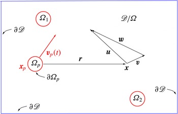
In the presence of a disperse phase, the carrier fluid fills the domain
 $\mathscr{D}\setminus {\it\Omega}$
, where
 $\mathscr{D}$
is the flow domain and
 ${\it\Omega}(t)=\cup _{p}{\it\Omega}_{p}(t)$
denotes the region occupied by the collection of
 $N_{p}$
rigid particles, with
 ${\it\Omega}_{p}(t)$
the time-dependent domain occupied by the
 $p$
th particle, see the sketch in figure 1. The set theoretic notation
 $\cup _{p}$
denotes the union of sets indexed by
 $p$
and
 $A\setminus B$
denotes the complement in
 $A$
of set
 $B$
. The motion of the carrier fluid is assumed to be described by the standard incompressible Navier–Stokes equations endowed with the no-slip condition at the particle boundaries:
 $$\begin{eqnarray}\left.\begin{array}{@{}c@{}}\left.\begin{array}{@{}c@{}}\boldsymbol{{\rm\nabla}}\boldsymbol{\cdot }\boldsymbol{u}=0,\\ \displaystyle \frac{\partial \boldsymbol{u}}{\partial t}+\boldsymbol{u}\boldsymbol{\cdot }\boldsymbol{{\rm\nabla}}\boldsymbol{u}=-\frac{1}{{\it\rho}_{f}}\boldsymbol{{\rm\nabla}}p+{\it\nu}{\rm\nabla}^{2}\boldsymbol{u},\end{array}\right\}\quad \boldsymbol{x}\in \mathscr{D}\setminus {\it\Omega}(t),\\ \boldsymbol{u}|_{\partial {\it\Omega}_{p}(t)}=\boldsymbol{V}_{p}(\boldsymbol{x})|_{\partial {\it\Omega}_{p}(t)},\quad p=1,\dots ,N_{p},\\ \boldsymbol{u}|_{\partial \mathscr{D}}=\boldsymbol{u}_{wall},\\ \boldsymbol{u}(\boldsymbol{x},0)=\boldsymbol{u}_{0}(\boldsymbol{x}),\quad \boldsymbol{x}\in \mathscr{D}\setminus {\it\Omega}(0).\end{array}\right\}\end{eqnarray}$$
In (2.1),
 $\boldsymbol{u}_{0}(\boldsymbol{x})$
is the velocity field at time
 $t=0$
,
 ${\it\rho}_{f}$
denotes the fluid density,
 ${\it\nu}$
is the kinematic viscosity,
 $\partial {\it\Omega}_{p}$
is the boundary of the
 $p$
th particle and
 $\partial \mathscr{D}$
is the boundary of the overall flow domain, see figure 1. In this microscopic description, the particles affect the carrier fluid through the no-slip condition at the moving particle surface
 $\partial {\it\Omega}_{p}(t)$
, where the fluid matches the local rigid-body velocity of the particle
 $\boldsymbol{V}_{p}(\boldsymbol{x})=\boldsymbol{v}_{p}+{\bf\omega}_{p}\times (\boldsymbol{x}-\boldsymbol{x}_{p})$
, with
 $\boldsymbol{v}_{p}$
the velocity of the particle geometric centre
 $\boldsymbol{x}_{p}(t)$
and
 ${\bf\omega}_{p}(t)$
the angular velocity. The equations of rigid-body dynamics need be coupled to the equation for the fluid velocity field to determine the particle motions, where the fluid stress vectors acting at the particle boundary provide the relevant forces and moments.
Sketch of the flow domain. The fluid fills the domain
 $\mathscr{D}\setminus {\it\Omega}$
, with
 ${\it\Omega}(t)=\cup _{p}{\it\Omega}_{p}(t)$
the region occupied by the
 $N_{p}$
rigid particles and
 ${\it\Omega}_{p}(t)$
the time-dependent domain of the
 $p$
th particle;
 $\partial \mathscr{D}$
denotes the boundary of
 $\mathscr{D}$
. The fluid velocity at the generic point
 $\boldsymbol{x}\in \mathscr{D}\setminus {\it\Omega}$
is decomposed as
 $\boldsymbol{u}=\boldsymbol{w}+\boldsymbol{v}$
, to be understood as the definition of
 $\boldsymbol{w}$
given the fluid velocity
 $\boldsymbol{u}$
and the solution
 $\boldsymbol{v}$
of the unsteady Stokes problem (2.4).

In principle, the system (2.1) can be numerically integrated at the price of resolving all the particle boundaries on the computational grid. When the suspension is formed by a huge number of small particles their direct solution is unaffordable. In any case, (2.1) still provides the basic description of the flow in terms of the interaction between the two phases. The purpose of the present subsection is to manipulate and approximate the basic equations to derive a viable model for the suspension.
As a starting point, for small time intervals
 $0\leqslant t\leqslant Dt$
, the carrier flow velocity is decomposed into two parts,
 $\boldsymbol{u}(\boldsymbol{x},t)=\boldsymbol{w}+\boldsymbol{v}$
. The field
 $\boldsymbol{w}(\boldsymbol{x},t)$
is assumed to satisfy the equations
 $$\begin{eqnarray}\left.\begin{array}{@{}c@{}}\boldsymbol{{\rm\nabla}}\boldsymbol{\cdot }\boldsymbol{w}=0,\\ \displaystyle \frac{\partial \boldsymbol{w}}{\partial t}+\boldsymbol{F}=-\frac{1}{{\it\rho}_{f}}\boldsymbol{{\rm\nabla}}{\rm\pi}+{\it\nu}{\rm\nabla}^{2}\boldsymbol{w},\\ \boldsymbol{w}|_{\partial \mathscr{D}}=\boldsymbol{u}_{wall}-\boldsymbol{v}_{\partial \mathscr{D}},\\ \boldsymbol{w}(\boldsymbol{x},0)=\bar{\boldsymbol{u}}_{0}(\boldsymbol{x}),\end{array}\right\}\end{eqnarray}$$
where
 $\boldsymbol{x}\in \mathscr{D}$
and
 $$\begin{eqnarray}\boldsymbol{F}=\left\{\begin{array}{@{}ll@{}}\boldsymbol{u}\boldsymbol{\cdot }\boldsymbol{{\rm\nabla}}\boldsymbol{u},\quad & \text{for}~\boldsymbol{x}\in \mathscr{D}\setminus {\it\Omega}(t),\\ \boldsymbol{V}_{p}\boldsymbol{\cdot }\boldsymbol{{\rm\nabla}}\boldsymbol{V}_{p},\quad & \text{for}~\boldsymbol{x}\in {\it\Omega}(t),\end{array}\right.\end{eqnarray}$$
is a field reproducing the complete convective term of the Navier–Stokes equation in the carrier fluid domain
 $\mathscr{D}\setminus {\it\Omega}$
, which is prolonged inside
 ${\it\Omega}$
using the solid particle velocity field. Other choices are possible, but the actual shape of the field inside the particle domains is irrelevant to our present purposes. In this respect, the solid body motion provides an elegant example given the continuity of the fluid velocity field
 $\boldsymbol{u}$
at the particle boundaries. In problem (2.2), apart from the prolongation of the field
 $\boldsymbol{F}$
, the particles disappear altogether from the domain, and the convective term, retaining its complete nonlinear nature in the fluid domain, is treated as a prescribed forcing term. The initial field
 $\bar{\boldsymbol{u}}_{0}$
is prolonged inside the particle domains by the same rule, i.e. the same rule as the solid body motion.
The field
 $\boldsymbol{v}(\boldsymbol{x},t)$
exactly satisfies the linear unsteady Stokes problem (the complete nonlinear term has been retained in the equation for
 $\boldsymbol{w}$
)
 $$\begin{eqnarray}\left.\begin{array}{@{}c@{}}\left.\begin{array}{@{}c@{}}\boldsymbol{{\rm\nabla}}\boldsymbol{\cdot }\boldsymbol{v}=0,\\ \displaystyle \frac{\partial \boldsymbol{v}}{\partial t}=-\frac{1}{{\it\rho}_{f}}\boldsymbol{{\rm\nabla}}\text{q}+{\it\nu}{\rm\nabla}^{2}\boldsymbol{v},\end{array}\right\}\quad \boldsymbol{x}\in \mathscr{D}\setminus {\it\Omega}(t),\\ \boldsymbol{v}|_{\partial {\it\Omega}_{p}(t)}=\boldsymbol{V}_{p}(\boldsymbol{x})~|_{\partial {\it\Omega}_{p}(t)}-\boldsymbol{w}|_{\partial {\it\Omega}_{p}(t)},\quad p=1,\dots ,N_{p},\\ \boldsymbol{v}(\boldsymbol{x},0)=0,\quad \boldsymbol{x}\in \mathscr{D}\setminus {\it\Omega}(0),\end{array}\right\}\end{eqnarray}$$
where the boundary conditions applied at the particle surfaces still couple the unsteady Stokes problem (2.4) with (2.2). It should be observed that no boundary conditions are applied to the field
 $\boldsymbol{v}$
at the flow domain boundary
 $\partial \mathscr{D}$
. In other words, the field
 $\boldsymbol{v}$
can be regarded as a free-space solution in the whole
 $\mathbb{R}^{3}$
restricted the actual flow domain
 $\mathscr{D}$
. Indeed, the value of
 $\boldsymbol{v}$
at the domain boundary is used to correct the boundary condition for
 $\boldsymbol{w}$
. It is worth calling the reader’s attention to the initial conditions for the two complementary problems: the initial velocity field is assigned as initial condition for
 $\boldsymbol{w}$
, leaving homogenous initial data for
 $\boldsymbol{v}$
. As shown in a later section, the homogeneous initial conditions for the perturbation field
 $\boldsymbol{v}$
will turn out to be a crucial feature of the decomposition.
The solution of (2.4) can be expressed in terms of the boundary integral representation of the unsteady Stokes equations which involves the unsteady Stokeslet
 $\unicode[STIX]{x1D60E}_{ij}(\boldsymbol{x},{\bf\xi},t,{\it\tau})$
, a second-order Cartesian tensor and the associated stresses in the form of the third-order tensor
 $\unicode[STIX]{x1D61B}_{ijk}(\boldsymbol{x},{\bf\xi},t,{\it\tau})$
, see §§ A.1 and A.2 and the classical textbooks by Zapryanov & Tabakova (Reference Zapryanov and Tabakova1998) and Kim & Karilla (Reference Kim and Karilla2005). The unsteady Stokeslet
 $\unicode[STIX]{x1D60E}_{ij}(\boldsymbol{x},{\bf\xi},t,{\it\tau})$
is readily interpreted as the fluid velocity (
 $i$
th direction) at position
 $\boldsymbol{x}$
and time
 $t$
due to the singular forcing
 ${\it\delta}(\boldsymbol{x}-{\bf\xi}){\it\delta}(t-{\it\tau})$
(
 $j$
th direction) applied at
 ${\bf\xi}$
at time
 ${\it\tau}$
. Exploiting the vanishing initial condition, the solution of (2.4) is recast in the boundary integral representation
 $$\begin{eqnarray}v_{i}(\boldsymbol{x},t)=\int _{0}^{t}\,\text{d}{\it\tau}\int _{\partial {\it\Omega}}t_{j}({\bf\xi},{\it\tau})\unicode[STIX]{x1D60E}_{ij}(\boldsymbol{x},{\bf\xi},t,{\it\tau})-v_{j}({\bf\xi},{\it\tau})\unicode[STIX]{x1D61B}_{ijk}(\boldsymbol{x},{\bf\xi},t,{\it\tau})n_{k}({\bf\xi})\,\text{d}S_{{\bf\xi}}.\end{eqnarray}$$
Equation (2.5) expresses
 $\boldsymbol{v}(\boldsymbol{x},t)$
in terms of a boundary integral on
 $\partial {\it\Omega}=\cup _{p}\partial {\it\Omega}_{p}$
involving the (physical) stress vector
 $t_{j}({\bf\xi},{\it\tau})$
and the boundary condition on the perturbation velocity
 $v_{j}({\bf\xi},{\it\tau})$
at each particle boundary. In principle, the stress vector
 $t_{j}({\bf\xi},{\it\tau})$
can be determined by solving the boundary integral equation (indeed, a system of coupled boundary integral equations, one for each particle) associated with representation (2.5). Once the stress vector is known at each particle boundary, representation (2.5) provides the perturbation field everywhere in the flow domain. Moreover, the boundary integral of the stress vector
 $t_{j}$
would provide the forces acting on the particles.
Since the present aim is to capture the effects of many small particles of diameter
 $d_{p}$
, the interest is focused on the far-field particle disturbance which can be approximated by a multipole expansion of (2.5). Substitution in (2.5) of the first-order truncation of the Taylor series of
 $\unicode[STIX]{x1D60E}_{ij}(\boldsymbol{x},{\bf\xi},t,{\it\tau})$
and
 $\unicode[STIX]{x1D61B}_{ijk}(\boldsymbol{x},{\bf\xi},t,{\it\tau})$
, centred at the particle position
 $\boldsymbol{x}_{p}$
, leads to the far-field expression for large
 $r_{p}/d_{p}$
, where
 $r_{p}=|\boldsymbol{x}-\boldsymbol{x}_{p}|$
,
 $$\begin{eqnarray}v_{i}(\boldsymbol{x},t)=-\mathop{\sum }_{p}\int _{0}^{t}D_{j}^{p}({\it\tau})\unicode[STIX]{x1D60E}_{ij}(\boldsymbol{x},\boldsymbol{x}_{p},t,{\it\tau})\,\text{d}{\it\tau},\end{eqnarray}$$
showing that the far-field disturbance depends only on the hydrodynamic force
 $\boldsymbol{D}_{p}({\it\tau})$
, with Cartesian components
 $D_{j}^{p}$
, which acts on the generic particle. Given the physical interpretation of the unsteady Stokeslet
 $\unicode[STIX]{x1D60E}_{ij}$
, the partial differential equation whose solution is given by (2.6) follows as
 $$\begin{eqnarray}\frac{\partial \boldsymbol{v}}{\partial t}-{\it\nu}{\rm\nabla}^{2}\boldsymbol{v}+\frac{1}{{\it\rho}_{f}}\boldsymbol{{\rm\nabla}}q=-\frac{1}{{\it\rho}_{f}}\mathop{\sum }_{p}\boldsymbol{D}_{p}(t)\,{\it\delta}[\boldsymbol{x}-\boldsymbol{x}_{p}(t)],\quad \boldsymbol{v}(\boldsymbol{x},0)=0,\end{eqnarray}$$
as is directly verified by combining the time derivative of (2.6) with its Laplacian. Consistently with the truncated multipole expansion (2.6) in (2.7), the fluid–particle coupling occurs via the (singular) forcing term in the unsteady Stokes problem and no boundary condition needs to be enforced at the particle surface. Actually, in the limit of small particles, the truncation of the multipole expansion implicitly provides for the boundary condition, which is rearranged as a forcing term in (2.7). Given the linearity, hereafter we shall explicitly consider the single contribution of the generic particle
 $p$
, keeping in mind that a final summation over all the particles is required. It is also clear that as the particle diameter gets smaller and smaller, the term
 $\boldsymbol{F}$
in (2.2) reduces to the standard convective terms of the Navier–Stokes equation
 $\boldsymbol{u}\boldsymbol{\cdot }\boldsymbol{{\rm\nabla}}\boldsymbol{u}$
, almost everywhere in
 $\mathscr{D}$
.
2.2. Disturbance flow due to a small particle
The vorticity equation associated with (2.7) is
 $$\begin{eqnarray}\frac{\partial {\bf\zeta}}{\partial t}-{\it\nu}{\rm\nabla}^{2}{\bf\zeta}=\frac{1}{{\it\rho}_{f}}\boldsymbol{D}_{p}(t)\times \boldsymbol{{\rm\nabla}}{\it\delta}[\boldsymbol{x}-\boldsymbol{x}_{p}(t)],\quad {\bf\zeta}(\boldsymbol{x},0)=0,\end{eqnarray}$$
where
 ${\bf\zeta}=\boldsymbol{{\rm\nabla}}\times \boldsymbol{v}$
. The solution can be expressed as a convolution with the fundamental solution of the diffusion equation
 $g(\boldsymbol{x}-{\bf\xi},t-{\it\tau})$
, given by (see § A.1)
 $$\begin{eqnarray}g(\boldsymbol{x}-{\bf\xi},t-{\it\tau})=\frac{1}{[4{\rm\pi}\,{\it\nu}(t-{\it\tau})]^{3/2}}\exp \left[-\frac{\Vert \boldsymbol{x}-{\bf\xi}\Vert ^{2}}{4{\it\nu}(t-{\it\tau})}\right],\end{eqnarray}$$
which is a Gaussian with time-dependent variance
 ${\it\sigma}(t-{\it\tau})=\sqrt{2{\it\nu}(t-{\it\tau})}$
. We observe that
 $g$
is the fundamental solution of the diffusion equation in free space, since
 $\boldsymbol{v}$
is itself a free-space field, as noted when discussing (2.4).
By rearranging the forcing on the right-hand side of (2.8) as a time convolution,
 $$\begin{eqnarray}\displaystyle & & \displaystyle \boldsymbol{D}_{p}(t)\times \boldsymbol{{\rm\nabla}}{\it\delta}[\boldsymbol{x}-\boldsymbol{x}_{p}(t)]=\int _{0}^{t^{+}}\boldsymbol{D}_{p}({\it\tau})\times \boldsymbol{{\rm\nabla}}{\it\delta}[\boldsymbol{x}-\boldsymbol{x}_{p}({\it\tau})]{\it\delta}(t-{\it\tau})\,\text{d}{\it\tau},\,\quad \nonumber\\ \displaystyle & & \displaystyle \quad \text{by}~\int _{0}^{t^{+}}f({\it\tau})\,\text{d}{\it\tau}~\text{we intend }\lim _{{\it\epsilon}\rightarrow 0}\int _{0}^{t+{\it\epsilon}}f({\it\tau})\,\text{d}{\it\tau},\end{eqnarray}$$
the solution of (2.8) follows at once as
 $$\begin{eqnarray}{\bf\zeta}(\boldsymbol{x},t)=\frac{1}{{\it\rho}_{f}}\int _{0}^{t^{+}}\boldsymbol{D}_{p}({\it\tau})\times \boldsymbol{{\rm\nabla}}g[\boldsymbol{x}-\boldsymbol{x}_{p}({\it\tau}),t-{\it\tau}]\,\text{d}{\it\tau}.\end{eqnarray}$$
The original fluid velocity
 $\boldsymbol{v}(\boldsymbol{x},t)$
can be reconstructed from the vorticity using the non-canonical decomposition
 $$\begin{eqnarray}\boldsymbol{v}(\boldsymbol{x},t)=\boldsymbol{v}_{{\bf\zeta}}(\boldsymbol{x},t)+\boldsymbol{{\rm\nabla}}{\it\phi}(\boldsymbol{x},t),\end{eqnarray}$$
where
 $$\begin{eqnarray}\boldsymbol{v}_{{\bf\zeta}}(\boldsymbol{x},t)=-\frac{1}{{\it\rho}_{f}}\int _{0}^{t^{+}}\boldsymbol{D}_{p}({\it\tau})g[\boldsymbol{x}-\boldsymbol{x}_{p}({\it\tau}),t-{\it\tau}]\,\text{d}{\it\tau}\end{eqnarray}$$
is a pseudo-velocity, such that its curl equals the vorticity,
 $\boldsymbol{{\rm\nabla}}\times \boldsymbol{v}_{{\bf\zeta}}={\bf\zeta}$
, and the gradient term is added to make the field solenoidal, as appropriate for incompressible flows,
 $$\begin{eqnarray}{\rm\nabla}^{2}{\it\phi}(\boldsymbol{x},t)=-\frac{1}{{\it\rho}_{f}}\int _{0}^{t^{+}}\boldsymbol{D}_{p}({\it\tau})\boldsymbol{\cdot }\boldsymbol{{\rm\nabla}}g[\boldsymbol{x}-\boldsymbol{x}_{p}({\it\tau}),t-{\it\tau}]\,\text{d}{\it\tau}.\end{eqnarray}$$
The pseudo-velocity
 $\boldsymbol{v}_{{\bf\zeta}}$
obeys the equation
 $$\begin{eqnarray}\frac{\partial \boldsymbol{v}_{{\bf\zeta}}}{\partial t}-{\it\nu}{\rm\nabla}^{2}\boldsymbol{v}_{{\bf\zeta}}=-\frac{1}{{\it\rho}_{f}}\boldsymbol{D}_{p}(t){\it\delta}[\boldsymbol{x}-\boldsymbol{x}_{p}(t)],\quad \boldsymbol{v}_{{\bf\zeta}}(\boldsymbol{x},0)=0.\end{eqnarray}$$
2.3. Regularization of the disturbance field due to a small particle
Both the velocity
 $\boldsymbol{v}$
and the vorticity
 ${\bf\zeta}$
are apparently singular, with singularity arising from the contribution to the integral near the upper integration limit,
 ${\it\tau}\simeq t$
, where
 $g(\boldsymbol{x}-{\bf\xi},t-{\it\tau})$
tends to behave as ‘badly’ as the Dirac delta function. On the contrary, away from the upper integration limit, the integrand is nicely behaved since it involves a Gaussian or its gradient.
In this subsection we define a regularization procedure based on a temporal cutoff
 ${\it\epsilon}_{R}$
such that the fields are additively split into a regular and a singular component. For instance, the decomposition of the vorticity reads
 $$\begin{eqnarray}{\bf\zeta}(\boldsymbol{x},t)={\bf\zeta}_{R}(\boldsymbol{x},t;{\it\epsilon}_{R})+{\bf\zeta}_{S}(\boldsymbol{x},t;{\it\epsilon}_{R}),\end{eqnarray}$$
with the smooth and singular parts respectively given by
 $$\begin{eqnarray}{\bf\zeta}_{R}(\boldsymbol{x},t)=\frac{1}{{\it\rho}_{f}}\int _{0}^{t-{\it\epsilon}_{R}}\boldsymbol{D}_{p}({\it\tau})\times \boldsymbol{{\rm\nabla}}g[\boldsymbol{x}-\boldsymbol{x}_{p}({\it\tau}),t-{\it\tau}]\,\text{d}{\it\tau}\end{eqnarray}$$
and
 $$\begin{eqnarray}{\bf\zeta}_{S}(\boldsymbol{x},t)=\frac{1}{{\it\rho}_{f}}\int _{t-{\it\epsilon}_{R}}^{t^{+}}\boldsymbol{D}_{p}({\it\tau})\times \boldsymbol{{\rm\nabla}}g[\boldsymbol{x}-\boldsymbol{x}_{p}({\it\tau}),t-{\it\tau}]\,\text{d}{\it\tau}.\end{eqnarray}$$
As implied by the fundamental solution of the diffusion equation, the regular part of the vorticity field is everywhere smooth and is characterized by the smallest spatial scale
 ${\it\sigma}_{R}={\it\sigma}({\it\epsilon}_{R})=\sqrt{2{\it\nu}{\it\epsilon}_{R}}$
. Thanks to the semigroup property of solutions of the diffusion equation, the regular field
 ${\bf\zeta}_{R}(\boldsymbol{x},t)$
can be interpreted as the free diffusion from time
 $t-{\it\epsilon}_{R}$
to time
 $t$
of the complete field at time
 $t-{\it\epsilon}_{R}$
,
 ${\bf\zeta}(\boldsymbol{x},t-{\it\epsilon}_{R})$
, namely
 $$\begin{eqnarray}{\bf\zeta}_{R}(\boldsymbol{x},t)=\int {\bf\zeta}({\bf\xi},t-{\it\epsilon}_{R})g(\boldsymbol{x}-{\bf\xi},{\it\epsilon}_{R})\,\text{d}{\bf\xi},\end{eqnarray}$$
where the spatial convolution integral propagates the field from
 $t-{\it\epsilon}_{R}$
to
 $t$
. Although physically obvious, (2.19) can be directly proved using the result
 $$\begin{eqnarray}g(\boldsymbol{x},t)=\int g({\bf\xi},t-{\it\epsilon}_{R})g(\boldsymbol{x}-{\bf\xi},{\it\epsilon}_{R})\,\text{d}{\bf\xi},\end{eqnarray}$$
which is nothing more that a re-expression of the semigroup property for the free-space diffusion equation applied to the fundamental solution
 $g$
. Actually, using the property (2.20) and introducing (2.11) at time
 $t-{\it\epsilon}_{R}$
into (2.19), after integration by parts, one readily obtains
 $$\begin{eqnarray}\displaystyle {\bf\zeta}_{R}(\boldsymbol{x},t) & = & \displaystyle \frac{1}{{\it\rho}_{f}}\int \left\{\int _{0}^{t-{\it\epsilon}_{R}}\boldsymbol{D}_{p}({\it\tau})\times \boldsymbol{{\rm\nabla}}_{{\bf\xi}}g[{\bf\xi}-\boldsymbol{x}_{p}({\it\tau}),t-{\it\epsilon}_{R}-{\it\tau}]\,\text{d}{\it\tau}\right\}g(\boldsymbol{x}-{\bf\xi},{\it\epsilon}_{R})\,\text{d}{\bf\xi}\nonumber\\ \displaystyle & = & \displaystyle \frac{1}{{\it\rho}_{f}}\int _{0}^{t-{\it\epsilon}_{R}}\boldsymbol{D}_{p}({\it\tau})\times \int \boldsymbol{{\rm\nabla}}_{{\bf\xi}}g[{\bf\xi}-\boldsymbol{x}_{p}({\it\tau}),t-{\it\epsilon}_{R}-{\it\tau}]g(\boldsymbol{x}-{\bf\xi},{\it\epsilon}_{R})\,\text{d}{\bf\xi}\,\text{d}{\it\tau}\nonumber\\ \displaystyle & = & \displaystyle \frac{1}{{\it\rho}_{f}}\int _{0}^{t-{\it\epsilon}_{R}}\boldsymbol{D}_{p}({\it\tau})\times \boldsymbol{{\rm\nabla}}\int g[{\bf\xi}-\boldsymbol{x}_{p}({\it\tau}),t-{\it\epsilon}_{R}-{\it\tau}]g(\boldsymbol{x}-{\bf\xi},{\it\epsilon}_{R})\,\text{d}{\bf\xi}\,\text{d}{\it\tau}\nonumber\\ \displaystyle & = & \displaystyle \frac{1}{{\it\rho}_{f}}\int _{0}^{t-{\it\epsilon}_{R}}\boldsymbol{D}_{p}({\it\tau})\times \boldsymbol{{\rm\nabla}}g[\boldsymbol{x}-\boldsymbol{x}_{p}({\it\tau}),t-{\it\tau}]\,\text{d}{\it\tau},\end{eqnarray}$$
which is indeed (2.17). The corresponding vorticity field
 ${\bf\zeta}_{R}$
at time
 $t$
obeys a forced diffusion equation where the forcing is applied at the slightly earlier time
 $t-{\it\epsilon}_{R}$
,
 $$\begin{eqnarray}\frac{\partial {\bf\zeta}_{R}}{\partial t}-{\it\nu}{\rm\nabla}^{2}{\bf\zeta}_{R}=-\frac{1}{{\it\rho}_{f}}\boldsymbol{{\rm\nabla}}\times \boldsymbol{D}_{p}(t-{\it\epsilon}_{R})g[\boldsymbol{x}-\boldsymbol{x}_{p}(t-{\it\epsilon}_{R}),{\it\epsilon}_{R}],\quad {\bf\zeta}_{R}(\boldsymbol{x},0)=0;\end{eqnarray}$$
see § A.3 for the detailed calculation. The velocity field
 $\boldsymbol{v}_{R}$
associated with the regularized vorticity field
 ${\bf\zeta}_{R}$
can be expressed though the general decomposition (2.12),
 $$\begin{eqnarray}\boldsymbol{v}_{R}(\boldsymbol{x},t)=\boldsymbol{v}_{{\bf\zeta}_{R}}+\boldsymbol{{\rm\nabla}}{\it\Phi}_{R},\end{eqnarray}$$
where, by analogy with (2.15), the regularized pseudo-velocity
 $\boldsymbol{v}_{{\bf\zeta}_{R}}$
is
 $$\begin{eqnarray}\frac{\partial \boldsymbol{v}_{{\bf\zeta}_{R}}}{\partial t}-{\it\nu}{\rm\nabla}^{2}\boldsymbol{v}_{{\bf\zeta}_{R}}=-\frac{1}{{\it\rho}_{f}}\boldsymbol{D}_{p}(t-{\it\epsilon}_{R})g[\boldsymbol{x}-\boldsymbol{x}_{p}(t-{\it\epsilon}_{R}),{\it\epsilon}_{R}],\quad \boldsymbol{v}_{{\bf\zeta}_{R}}(\boldsymbol{x},0)=0,\end{eqnarray}$$
and the potential correction follows from the equation
 $$\begin{eqnarray}{\rm\nabla}^{2}{\it\Phi}_{R}=-\boldsymbol{{\rm\nabla}}\boldsymbol{\cdot }\boldsymbol{v}_{{\bf\zeta}_{R}}.\end{eqnarray}$$
It is worth noticing that the complete regularized field obeys instead the forced unsteady Stokes equation
 $$\begin{eqnarray}\frac{\partial \boldsymbol{v}_{R}}{\partial t}-{\it\nu}{\rm\nabla}^{2}\boldsymbol{v}_{R}+\frac{1}{{\it\rho}_{f}}\boldsymbol{{\rm\nabla}}q_{R}=-\frac{1}{{\it\rho}_{f}}\boldsymbol{D}_{p}(t-{\it\epsilon}_{R})\,g[\boldsymbol{x}-\boldsymbol{x}_{p}(t-{\it\epsilon}_{R}),{\it\epsilon}_{R}]\end{eqnarray}$$
for the solenoidal field
 $\boldsymbol{v}_{R}$
. The crucial point to observe here is that the regularized component of the velocity disturbance
 $\boldsymbol{v}_{R}(\boldsymbol{x},t)$
evolves according to a diffusion equation forced by the anticipating Stokes drag (i.e. evaluated at
 $t-{\it\epsilon}_{R}$
) times the regular spatial distribution
 $g[\boldsymbol{x}-\boldsymbol{x}_{p}(t-{\it\epsilon}_{R}),{\it\epsilon}_{R}]$
. Equation (2.24) can, in principle, be straightforwardly solved on a discrete grid, once the spatial scale
 ${\it\sigma}_{R}$
of the forcing is properly resolved by the grid. Once
 $\boldsymbol{v}_{{\bf\zeta}_{R}}$
is known, the correction needed to make the field solenoidal calls for the solution of the Poisson equation (2.25).
For the future application to the full solver for the carrier phase in the presence of the suspension, it is also worth mentioning that the field
 $\boldsymbol{v}_{{\bf\zeta}_{R}}$
is rapidly decaying in space as long as the observation time
 $t$
is small, since it implies the short-time diffusion of a rapidly decaying forcing. All the long-range effects are indeed confined to the potential correction
 $\boldsymbol{{\rm\nabla}}{\it\Phi}_{R}$
. As will be discussed in the forthcoming sections, the field
 $\boldsymbol{v}_{R}$
does not need to be separately evaluated, since it will be embedded in the solution procedure for the single field
 $\boldsymbol{u}$
which accounts for both the undisturbed carrier flows and the particle perturbation.
At variance with
 $\boldsymbol{v}_{R}$
, the singular contribution
 $\boldsymbol{v}_{S}$
cannot be represented on a discrete grid. It can also be decomposed into a vorticity related component plus a potential correction, according to the general representation (2.12). The vortical component
 $\boldsymbol{v}_{{\bf\zeta}_{S}}$
is an extremely rapidly decaying function of distance from the actual position of the particle, while its potential correction
 $\boldsymbol{{\rm\nabla}}{\it\Phi}_{S}$
is not. In order to address the error propagation of the algorithm that will be illustrated in the next section, it is instrumental to explicitly provide an estimate on the order of magnitude of the field
 $\boldsymbol{{\rm\nabla}}{\it\Phi}_{S}$
. The singular part of the pseudo-velocity is given by
 $$\begin{eqnarray}\boldsymbol{v}_{{\bf\zeta}_{S}}(\boldsymbol{x},t)=\frac{1}{{\it\rho}_{f}}\int _{t-{\it\epsilon}_{R}}^{t^{+}}\boldsymbol{D}_{p}({\it\tau})g[\boldsymbol{x}-\boldsymbol{x}_{p}({\it\tau}),t-{\it\tau}]\,\text{d}{\it\tau};\end{eqnarray}$$
see (2.13) for comparison. The equation for the potential correction is then
 $$\begin{eqnarray}{\rm\nabla}^{2}{\it\Phi}_{S}=-\boldsymbol{{\rm\nabla}}\boldsymbol{\cdot }\boldsymbol{v}_{{\bf\zeta}_{S}}=\frac{1}{{\it\rho}_{f}}\int _{t-{\it\epsilon}_{R}}^{t^{+}}\boldsymbol{D}_{p}({\it\tau})\boldsymbol{\cdot }\boldsymbol{{\rm\nabla}}g[\boldsymbol{x}-\boldsymbol{x}_{p}({\it\tau}),t-{\it\tau}]\,\text{d}{\it\tau}.\end{eqnarray}$$
It follows that
 $$\begin{eqnarray}{\it\Phi}_{S}=-\frac{1}{{\it\rho}_{f}}\int _{t-{\it\epsilon}_{R}}^{t^{+}}\,\text{d}{\it\tau}\boldsymbol{D}_{p}({\it\tau})\boldsymbol{\cdot }\boldsymbol{{\rm\nabla}}\int _{\mathbb{R}^{3}}\frac{g[\boldsymbol{y}-\boldsymbol{x}_{p}({\it\tau}),t-{\it\tau}]}{4{\rm\pi}|\boldsymbol{x}-\boldsymbol{y}|}\,\text{d}^{3}\boldsymbol{y},\end{eqnarray}$$
where
 $-1/(4{\rm\pi}|\boldsymbol{x}-\boldsymbol{y}|)$
is the fundamental solution of the Laplace equation. From the solution (2.29) a rough estimate for the correction field
 $\boldsymbol{{\rm\nabla}}{\it\Phi}_{S}$
is immediately obtained as
 $$\begin{eqnarray}|\boldsymbol{{\rm\nabla}}{\it\Phi}_{S}|\leqslant \frac{1}{{\it\rho}_{f}}\sup _{t-{\it\epsilon}_{R}\leqslant {\it\tau}\leqslant t^{+}}|\boldsymbol{D}_{p}|\left|\boldsymbol{{\rm\nabla}}\otimes \boldsymbol{{\rm\nabla}}\int _{\mathbb{R}^{3}}\frac{\displaystyle \int _{t-{\it\epsilon}_{R}}^{t^{+}}g[\boldsymbol{y}-\boldsymbol{x}_{p}({\it\tau}),t-{\it\tau}]\,\text{d}{\it\tau}}{4{\rm\pi}|\boldsymbol{x}-\boldsymbol{y}|}\,\text{d}^{3}\boldsymbol{y}\right|.\end{eqnarray}$$
Sufficiently far away from the particle, i.e.
 $|\boldsymbol{x}-\boldsymbol{x}_{p}|/d_{p}\gg 1$
, the above estimate is asymptotically expressed as
 $$\begin{eqnarray}\displaystyle |\boldsymbol{{\rm\nabla}}{\it\Phi}_{S}|\leqslant \frac{1}{{\it\rho}_{f}}\int _{\mathbb{R}^{3}}\int _{t-{\it\epsilon}_{R}}^{t^{+}}g[\boldsymbol{y}-\boldsymbol{x}_{p}({\it\tau}),t-{\it\tau}]\,\text{d}{\it\tau}\,\text{d}^{3}\boldsymbol{y}\sup _{t-{\it\epsilon}_{R}\leqslant {\it\tau}\leqslant t^{+}}|\boldsymbol{D}_{p}|\left|\boldsymbol{{\rm\nabla}}\otimes \boldsymbol{{\rm\nabla}}\frac{1}{4{\rm\pi}|\boldsymbol{x}-\boldsymbol{x}_{p}^{\ast }|}\right|, & & \displaystyle \nonumber\\ \displaystyle & & \displaystyle\end{eqnarray}$$
where
 $\boldsymbol{x}_{p}^{\ast }=\boldsymbol{x}_{p}({\it\tau}^{\ast })$
,
 $t-{\it\epsilon}_{R}\leqslant {\it\tau}^{\ast }\leqslant t^{+}$
, is the position along the portion of the particle trajectory closest to the point
 $\boldsymbol{x}$
. Given the known integral
 $$\begin{eqnarray}\int _{\mathbb{R}^{3}}\frac{1}{(2{\rm\pi}{\it\sigma}^{2})^{3/2}}\text{e}^{-r^{2}/(2{\it\sigma}^{2})}\,\text{d}^{3}\boldsymbol{r}=1,\end{eqnarray}$$
one ends up with
 $$\begin{eqnarray}|\boldsymbol{{\rm\nabla}}{\it\Phi}_{S}|\leqslant \sup _{t-{\it\epsilon}_{R}\leqslant {\it\tau}\leqslant t^{+}}|\boldsymbol{D}_{p}|\frac{{\it\epsilon}_{R}}{4{\rm\pi}{\it\rho}_{f}|\boldsymbol{x}-\boldsymbol{x}_{p}^{\ast }|^{3}},\end{eqnarray}$$
where the norm of the double tensor
 $\boldsymbol{{\rm\nabla}}\otimes \boldsymbol{{\rm\nabla}}[1/(4{\rm\pi}|\boldsymbol{x}-\boldsymbol{x}_{p}^{\ast })]$
is given by
 $$\begin{eqnarray}\left|\boldsymbol{{\rm\nabla}}\otimes \boldsymbol{{\rm\nabla}}\frac{1}{4{\rm\pi}|\boldsymbol{x}-\boldsymbol{x}_{p}^{\ast }|}\right|=\sup _{|\hat{\boldsymbol{e}}|=1}\left[(\hat{\boldsymbol{e}}\boldsymbol{\cdot }\boldsymbol{{\rm\nabla}})\boldsymbol{{\rm\nabla}}\frac{1}{4{\rm\pi}|\boldsymbol{x}-\boldsymbol{x}_{p}^{\ast }|}\right]=\frac{1}{4{\rm\pi}|\boldsymbol{x}-\boldsymbol{x}_{p}^{\ast }|^{3}}.\end{eqnarray}$$
From the expression of the singular component of the pseudo-velocity (2.27) it is clear that, far from the particle,
 $\boldsymbol{v}_{{\bf\zeta}_{S}}$
decays exponentially fast, hence the far-field dominating component of
 $\boldsymbol{v}_{S}$
is provided by the long-range correction
 $\boldsymbol{{\rm\nabla}}{\it\Phi}_{S}$
that is of order
 ${\it\epsilon}_{R}/r^{3}$
. It is also clear that close to the particle the singular contribution is unbounded. This singular near field is however unessential as far as the relevant length scales of the system are concerned, as either the smallest hydrodynamic scale
 ${\it\eta}$
or the inter-particle distance is larger than
 ${\it\sigma}_{R}=\sqrt{2{\it\nu}{\it\epsilon}_{R}}$
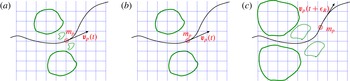
. For this reason, it will be neglected when advancing the solution by one time step in the actual algorithm illustrated in the following sections. However, this highly localized field will eventually diffuse to larger scales at later times. Hence, the singular contribution that is neglected during a single time step is successively reintroduced into the field as soon as it reaches the smallest physically relevant scales of the system. This procedure guarantees that the error does not accumulate in time, thereby maintaining the accuracy of the calculation. Figure 2 sketches the decomposition into regular and singular fields, using the vorticity field to describe the process as it is easier to visualize than the velocity field. The sketch highlights the singular production of vorticity by the particle, its diffusion, associated with the momentum transfer to the fluid, and the regularizing effects of viscosity. A crucial point is that the singular component of the field, which cannot be represented on a discrete mesh, is fully recovered at a successive time instant when its characteristic length scale reaches the grid size. In the following section the convective effect of the singular field will be dealt with in more detail, to show that it is indeed negligible when the dynamics is observed at the relevant hydrodynamical scale.
The coupling mechanism and regularization procedure. The green curves sketch the vorticity field. (a) The complete vorticity field generated by the particle at the current time
 $t$
is split into the regular
 ${\bf\zeta}_{R}(\boldsymbol{x},t)$
(solid green line) and singular
 ${\bf\zeta}_{S}(\boldsymbol{x},t)$
(dashed green line) components respectively. (b) Only the regular component
 ${\bf\zeta}_{R}(\boldsymbol{x},t)$
can be represented by the computational grid with mesh size
 $Dx$
at the generic time
 $t$
. (c) After the elapsed time
 ${\it\epsilon}_{R}$
(time
 $t+{\it\epsilon}_{R}$
) the singular component of the vorticity field diffuses to scales large enough to be captured by the discrete grid. The momentum transfer towards the fluid occurs via viscous diffusion of the vorticity generated by the particle. When only the regularized field is considered, a small error is incurred in the exchanged momentum. However, the successive diffusion of the singular field fully recovers the correct amount of vorticity at a successive time step. Thus, the error does not accumulate in time and remains under control along the simulation.

2.4. Coupling with the carrier flow
The regularized fluid velocity of the carrier flow in the presence of the perturbing particles is obtained by aggregating the two contributions of the velocity decomposition
 $\boldsymbol{u}_{R}=\boldsymbol{w}+\boldsymbol{v}_{R}$
described in § 2.1. The resulting field obeys the equations
 $$\begin{eqnarray}\displaystyle \left.\begin{array}{@{}c@{}}\boldsymbol{{\rm\nabla}}\boldsymbol{\cdot }\boldsymbol{u}_{R}=0,\\ \displaystyle \frac{\partial \boldsymbol{u}_{R}}{\partial t}+\boldsymbol{u}_{R}\boldsymbol{\cdot }\boldsymbol{{\rm\nabla}}\boldsymbol{u}_{R}+\left\{\boldsymbol{v}_{S}\boldsymbol{\cdot }\boldsymbol{{\rm\nabla}}\boldsymbol{u}_{R}+\boldsymbol{u}_{R}\boldsymbol{\cdot }\boldsymbol{{\rm\nabla}}\boldsymbol{v}_{S}+\boldsymbol{v}_{S}\boldsymbol{\cdot }\boldsymbol{{\rm\nabla}}\boldsymbol{v}_{S}\right\}\\ =\displaystyle -\frac{1}{{\it\rho}_{f}}\boldsymbol{{\rm\nabla}}p+{\it\nu}{\rm\nabla}^{2}\boldsymbol{u}_{R}-\frac{1}{{\it\rho}_{f}}\mathop{\sum }_{p}^{N_{p}}\boldsymbol{D}_{p}(t-{\it\epsilon}_{R})\,g[\boldsymbol{x}-\boldsymbol{x}_{p}(t-{\it\epsilon}_{R}),{\it\epsilon}_{R}],\end{array}\right\} & & \displaystyle \nonumber\\ \displaystyle & & \displaystyle\end{eqnarray}$$
with boundary and initial conditions given by
 $$\begin{eqnarray}\boldsymbol{u}_{R}|_{\partial \mathscr{D}}=\boldsymbol{u}_{wall}-\boldsymbol{v}_{S}|_{\partial \mathscr{D}},\quad \boldsymbol{u}_{R}(\boldsymbol{x},0)=\boldsymbol{u}_{0}(\boldsymbol{x}),\end{eqnarray}$$
where we have added the contributions arising from all the
 $N_{p}$
particles transported by the fluid. It should be stressed that the boundary condition for the regularized velocity
 $\boldsymbol{u}_{R}$
at
 $\partial \mathscr{D}$
needs the singular contribution
 $\boldsymbol{v}_{S}$
to be taken into account.
An interpretation of (2.35) could now be helpful. Along its motion the particle experiences the hydrodynamic force. In the formulation here proposed, the force is naturally regularized by viscous diffusion, hence the mollified Dirac delta functions takes the form of the fundamental solution of the diffusion equation. The effect of the hydrodynamic force is the generation of the regularized vorticity, (2.17), which is characterized by the smallest length scale
 ${\it\sigma}_{R}=\sqrt{2{\it\nu}{\it\epsilon}_{R}}$
, where
 ${\it\epsilon}_{R}$
is the regularization diffusion time scale. A crucial point to be stressed again is that the hydrodynamic forcing acting on the regularized solution at time
 $t$
is the one experienced by the particles at a slightly previous time
 $t-{\it\epsilon}_{R}$
when their position was
 $\boldsymbol{x}_{p}(t-{\it\epsilon}_{R})$
. The net effect of the disperse phase on the regularized carrier flow field is then accounted for by the extra forcing term corresponding to the time-delayed hydrodynamic force, expressed as the Gaussian
 $g[\boldsymbol{x}-\boldsymbol{x}_{p}(t-{\it\epsilon}_{R}),{\it\epsilon}_{R}]$
with variance
 ${\it\sigma}_{R}$
.
The total field
 $\boldsymbol{u}$
will involve a singular part that is concentrated on scales smaller than the physically relevant ones. As such, the singular contribution is actually neglected since only the regularized field needs to be considered. However, contributions from the singular disturbance field
 $\boldsymbol{v}_{S}$
appear in the term in curly brackets in (2.35). Indeed, in the far field of the particles
 $\boldsymbol{v}_{S}$
was already shown to be of the order of
 ${\it\epsilon}_{R}/r^{3}$
, which is negligible in comparison with the other terms in the equation. It is worth recalling that, at the successive time step, the corresponding contribution is reintroduced into the field, giving rise to no error accumulation in the long run. The crucial point here is that (2.35) is taken to hold almost everywhere in
 $\mathscr{D}$
near the particle position
 $\boldsymbol{x}_{p}$
. In this near field the term in curly brackets needs to be treated with some care. In fact, due to the scale separation between
 $\boldsymbol{u}_{R}$
and
 $\boldsymbol{v}_{S}$
, the filtering of the fields on a scale
 ${\it\Delta}$
that is of the order of the smallest hydrodynamic scale does not alter
 $\boldsymbol{u}_{R}$
, i.e. denoting by
 $\hat{\boldsymbol{u}}_{R}$
the filtered field one has
 $\boldsymbol{u}_{R}=\hat{\boldsymbol{u}}_{R}$
. In such conditions the equations for the regularized field follow by applying the filter to the system (2.35). As a result of scale separation, the filter is actually acting only on the terms in curly brackets which involve the singular contribution
 $\boldsymbol{v}_{S}$
. As explicitly shown in § A.4, a few detailed calculations show that the filtered terms give a contribution of the order
 $$\begin{eqnarray}\left.\begin{array}{@{}c@{}}\displaystyle \widehat{\boldsymbol{v}_{S}\boldsymbol{\cdot }\boldsymbol{{\rm\nabla}}\boldsymbol{v}_{S}}\sim \mathit{Re}_{p}\left(\frac{{\it\sigma}_{R}}{{\it\Delta}}\right)^{3}\frac{\boldsymbol{D}_{p}}{{\it\rho}_{f}}g_{max},\\ \displaystyle \widehat{\boldsymbol{v}_{S}\boldsymbol{\cdot }\boldsymbol{{\rm\nabla}}\boldsymbol{u}_{R}}\sim \widehat{\boldsymbol{u}_{R}\boldsymbol{\cdot }\boldsymbol{{\rm\nabla}}\boldsymbol{v}_{S}}\sim \mathit{Re}_{p}\left(\frac{{\it\sigma}_{R}}{{\it\Delta}}\right)^{2}\frac{\boldsymbol{D}_{p}}{{\it\rho}_{f}}g_{max},\end{array}\right\}\end{eqnarray}$$
where
 $g_{max}=1/(2{\rm\pi}{\it\sigma}_{R}^{2})^{3/2}$
is the maximum of the mollified delta function. Clearly, the above filtered convective terms are an order
 $\mathit{Re}_{p}$
smaller than the forcing term on the right-hand side of (2.35). Under the assumption of small particle Reynolds number they can be safely neglected in the evolution equation of the regularized field.
We would like to stress the simplicity of the final equations that have to be solved,
 $$\begin{eqnarray}\left.\begin{array}{@{}c@{}}\boldsymbol{{\rm\nabla}}\boldsymbol{\cdot }\boldsymbol{u}_{R}=0,\\ \displaystyle \frac{\partial \boldsymbol{u}_{R}}{\partial t}+\boldsymbol{u}_{R}\boldsymbol{\cdot }\boldsymbol{{\rm\nabla}}\boldsymbol{u}_{R}=-\frac{1}{{\it\rho}_{f}}\boldsymbol{{\rm\nabla}}p+{\it\nu}{\rm\nabla}^{2}\boldsymbol{u}_{R}-\frac{1}{{\it\rho}_{f}}\mathop{\sum }_{p}^{N_{p}}\boldsymbol{D}_{p}(t-{\it\epsilon}_{R})\,g[\boldsymbol{x}-\boldsymbol{x}_{p}(t-{\it\epsilon}_{R}),{\it\epsilon}_{R}].\end{array}\right\}\end{eqnarray}$$
The effect of the disperse phase on the carrier fluid is taken into account by an extra term in the Navier–Stokes equations. Under this point of view, any standard Navier–Stokes solver can be easily equipped with such an extra term which is known in closed form. Furthermore, each particle will produce an active forcing on the fluid localized in a sphere of radius order
 ${\it\sigma}_{R}$
centred at the particle position. In the presence of many particles only the few grid points in the sphere of influence of the particle will receive the disturbance produced by the particle itself. Finally, the forcing term is grid-independent in the sense that, once the grid spacing is refined (
 $Dx$
progressively getting smaller at fixed
 ${\it\sigma}_{R}$
), any successively finer grid will only provide a better numerical approximation of the same forcing.
2.5. Evaluation of the hydrodynamic force and removal of self-interaction
The dynamics of a point particle of mass
 $m_{p}$
in the relative motion with respect to a Newtonian fluid is described by the equation of motion
 $$\begin{eqnarray}\frac{\text{d}\boldsymbol{x}_{p}}{\text{d}t}=\boldsymbol{v}_{p}(t),\quad m_{p}\frac{\text{d}\boldsymbol{v}_{p}}{\text{d}t}=\boldsymbol{D}_{p}(t)+(m_{p}-m_{f})\boldsymbol{g},\end{eqnarray}$$
where
 $m_{f}$
is the displaced mass of fluid,
 $\boldsymbol{D}_{p}(t)$
is the hydrodynamic force and
 $\boldsymbol{g}$
is the acceleration due to gravity. Clearly, for the accurate evaluation of the particle trajectories and of the inter-phase momentum coupling, an accurate and efficient expression for the hydrodynamic force is mandatory. To obtain such an expression one should reconsider the equation for the perturbation field
 $\boldsymbol{v}$
addressed in § 2.1.
As shown there, the perturbation due to the presence of a particle obeys the unsteady Stokes equation (2.4) where, worthy of note, the initial condition for the perturbation field
 $\boldsymbol{v}$
is homogeneous. Indeed, in our scheme, the solution of the unsteady Stokes equation for
 $\boldsymbol{v}$
at the generic time step provides the stress at the fluid–particle interface and ultimately yields the drag force. Luckily, there is no need to work out the details, since Maxey & Riley (Reference Maxey and Riley1983) have already provided the expression for the general unsteady drag force of a spherical particle when the field has homogenous initial conditions, which is the case of interest here. Their solution can in fact be fully exploited to provide the drag force for the perturbation flow which is asymptotically expressed as (2.6) during the generic time step.
Following Maxey & Riley (Reference Maxey and Riley1983), the force
 $\boldsymbol{D}_{p}(t)$
can be evaluated as
 $$\begin{eqnarray}\displaystyle \boldsymbol{D}_{p}(t) & = & \displaystyle 6{\rm\pi}{\it\mu}a_{p}\left[\tilde{\boldsymbol{u}}(\boldsymbol{x}_{p},t)+\frac{a_{p}^{2}}{6}{\rm\nabla}^{2}\tilde{\boldsymbol{u}}(\boldsymbol{x}_{p},t)-\boldsymbol{v}_{p}(t)\right]\nonumber\\ \displaystyle & & \displaystyle +\,m_{f}\frac{\text{D}\tilde{\boldsymbol{u}}}{\text{D}t}\bigg|_{x_{p}}+\frac{1}{2}m_{f}\frac{\text{d}}{\text{d}t}\left[\tilde{\boldsymbol{u}}(\boldsymbol{x}_{p},t)+\frac{a_{p}^{2}}{10}{\rm\nabla}^{2}\tilde{\boldsymbol{u}}(\boldsymbol{x}_{p},t)-\boldsymbol{v}_{p}(t)\right]+6{\rm\pi}{\it\mu}a_{p}^{2}\nonumber\\ \displaystyle & & \displaystyle \times \int _{0}^{t}\,\text{d}{\it\tau}\,\frac{1}{[{\rm\pi}{\it\nu}(t-{\it\tau})]^{1/2}}\frac{\text{d}}{\text{d}{\it\tau}}\left[\tilde{\boldsymbol{u}}(\boldsymbol{x}_{p},{\it\tau})+\frac{a_{p}^{2}}{6}{\rm\nabla}^{2}\tilde{\boldsymbol{u}}(\boldsymbol{x}_{p},{\it\tau})-\boldsymbol{v}_{p}({\it\tau})\right],\end{eqnarray}$$
where
 $a_{p}=d_{p}/2$
is the particle radius. Expression (2.40) involves the steady Stokes drag (first line), the added mass terms (second line) and the Basset history force (third line). In all terms the Faxen correction associated with spatial non-uniformity of the flow is included and, following the original derivation by Maxey & Riley (Reference Maxey and Riley1983), the velocity
 $\tilde{\boldsymbol{u}}(\boldsymbol{x}_{p},t)$
must be interpreted as the fluid velocity, at the particle position, in the absence of the particle self-interaction, i.e.
 $\tilde{\boldsymbol{u}}_{p}$
should account for the background, possibly turbulent, flow and for the disturbance generated by all the other particles except the
 $p$
th one; see also Gatignol (Reference Gatignol1983) and Boivin, Simonin & Squires (Reference Boivin, Simonin and Squires1998). In the regime of our interest, where the particle backreaction modifies the carrier flow, the correct calculation of
 $\tilde{\boldsymbol{u}}_{p}$
is crucial and calls for an effective procedure to remove from the field
 $\boldsymbol{u}(\boldsymbol{x},t)$
the particle self-interaction contribution evaluated at the particle position. Luckily, the (regularized) disturbance flow generated by each particle is known in closed form and can thus be easily removed from the complete field in computing the hydrodynamic force, at least for numerical algorithms using explicit time integration schemes. As an illustration, let us consider the simple case of heavy small particles,
 ${\it\rho}_{p}\gg {\it\rho}_{f}$
, where the hydrodynamic force (2.40) reduces to the Stokes drag
 $$\begin{eqnarray}\boldsymbol{D}_{p}(t)=6{\rm\pi}{\it\mu}a_{p}[\tilde{\boldsymbol{u}}(\boldsymbol{x}_{p},t)-\boldsymbol{v}_{p}(t)].\end{eqnarray}$$
The explicit calculation of the velocity
 $\boldsymbol{v}_{R}(\boldsymbol{x}-\boldsymbol{x}_{0},t)$
induced at time
 $t$
and position
 $\boldsymbol{x}$
by a particle located at
 $\boldsymbol{x}_{0}$
is provided in § A.5. This result can be exploited to remove the self-interaction term in the illustrative case of an explicit Euler time advancement algorithm. Indeed, in this case, to correctly evaluate the right-hand side of (2.41) it suffices to subtract from
 $\boldsymbol{u}(\boldsymbol{x}_{p},t)$
the value
 $\boldsymbol{v}_{R}[\boldsymbol{x}_{p}(t)-\boldsymbol{x}_{p}(t-Dt),Dt]$
induced at time
 $t$
at the current particle position
 $\boldsymbol{x}_{p}(t)$
by the same particle when it was placed at
 $\boldsymbol{x}_{p}(t-Dt)$
. The same kind of reasoning can be straightforwardly extended to other explicit time integration schemes, e.g. to each intermediate step of a Runge–Kutta algorithm and to the different contributions in the general expression of the force (2.40), e.g. bubbly flows (Climent & Magnaudet Reference Climent and Magnaudet2006).
Before closing this section devoted to force evaluation, a final note is in order concerning the Basset force: it represents the effects on the force due to the particle–fluid interaction during the previous motion of the particle before the actual time
 $t$
. In cases where the particle does not modify the carrier flow, see the derivation by Maxey & Riley (Reference Maxey and Riley1983), this interaction is modelled by a memory convolution integral which mimics the particle vorticity production and its viscous diffusion occurring from the initial time
 $t=0$
up to the actual time
 $t$
. In our case, the carrier fluid is perturbed step-by-step by the particle motion (two-way coupling regime) and the diffusion of the vorticity produced by the particle during the past motion before the actual time
 $t$
is captured without any modelling by (2.38). Hence, the time integral must model only the vorticity production occurring during the last time step
 $Dt$
, i.e. the memory integral is limited to a single time step of the eventual integration algorithm. Actually, the effects of the previous history come in through the boundary condition of (2.4), where the field
 $\boldsymbol{w}$
must be interpreted as the background velocity acting on the particle, i.e. as the carrier flow velocity field that would occur at the particle boundary during the last time step in the absence of the particle. For small particles this field reduces to the value at the particle centre plus a Faxen-like correction accounting for spatial flow variations on the scale of the particle.
3. Algorithm validation
The methodology illustrated in the previous sections needs to be validated. We will address several test cases where analytical data can be employed for comparison. To better focus our attention on the interaction between the fluid and the disperse phase, we will consider a periodic box
 $\mathscr{D}$
free from solid boundaries which may hinder the analysis. The numerical solution of (2.26) and (2.35) for the carrier fluid is based on a pseudo-spectral Fourier-based spatial discretization where the nonlinear terms are calculated by the standard
 $3/2$
dealiasing procedure. Time advancement is achieved by a low-storage semi-implicit Runge–Kutta method with a fourth-order Adams–Bashforth formulation for the convective terms and an implicit Crank–Nicolson formula for the diffusive terms. The details of the implementation are described elsewhere, see Gualtieri et al. (Reference Gualtieri, Casciola, Benzi, Amati and Piva2002).
3.1. Response to a localized force
We start by addressing a simple case where a known small-amplitude constant force
 $\boldsymbol{F}$
is applied at a fixed point
 $\boldsymbol{x}_{p}$
to the fluid which is initially at rest in the domain
 $\mathscr{D}$
. Due to the small amplitude of the forcing, the flow obeys the linear unsteady Stokes equations (2.7) which are suitable for an analytical solution. It is useful to fix the notation: the constant force has Cartesian components
 $\boldsymbol{F}=(F_{x},F_{y},F_{z})$
, the corresponding velocity vector is
 $\boldsymbol{u}=(u,v,w)$
and the distance from
 $\boldsymbol{x}_{p}$
is measured by the vector
 $\boldsymbol{r}=\boldsymbol{x}-\boldsymbol{x}_{p}$
, whose Cartesian components are
 $\boldsymbol{r}=(r_{x},r_{y},r_{z})$
. Hereafter, we will consider the force in the
 $x$
direction, namely
 $\boldsymbol{F}=(F_{0},0,0)$
. In fact, an exact solution can be easily determined in closed form by evaluating the time convolution integral between the unsteady Green tensor, see § A.2 equation (A 13), and the force
 $\boldsymbol{F}$
. After some algebra, the fluid velocity in the direction of the force when
 $\boldsymbol{r}=(r_{x},0,0)$
reads
 $$\begin{eqnarray}u(r_{x},t)=\frac{F_{0}}{{\it\mu}\sqrt{4{\it\nu}t}}\frac{1}{4{\rm\pi}}\left[\frac{1}{2{\it\eta}_{t}^{3}}\text{erf}({\it\eta}_{t})-\frac{1}{2{\it\eta}_{t}}\text{erf}({\it\eta}_{t})-\frac{1}{\sqrt{{\rm\pi}}{\it\eta}_{t}^{2}}\exp (-{\it\eta}_{t}^{2})+\frac{1}{{\it\eta}_{t}}\right],\end{eqnarray}$$
while for
 $\boldsymbol{r}=(0,r_{y},0)$
it reads
 $$\begin{eqnarray}u(r_{y},t)=\frac{F_{0}}{{\it\mu}\sqrt{4{\it\nu}t}}\frac{1}{8{\rm\pi}}\left[-\frac{1}{2{\it\eta}_{t}^{3}}\text{erf}({\it\eta}_{t})-\frac{1}{{\it\eta}_{t}}\text{erf}({\it\eta}_{t})+\frac{1}{\sqrt{{\rm\pi}}{\it\eta}_{t}^{2}}\exp (-{\it\eta}_{t}^{2})+\frac{1}{{\it\eta}_{t}}\right],\end{eqnarray}$$
where
 ${\it\eta}_{t}=r/\sqrt{4{\it\nu}t}$
and
 $r=\sqrt{r_{k}\,r_{k}}$
. The expressions (3.1) and (3.2) highlight that the response of the fluid to a concentrated force assumes a self-similar form when the velocity is rescaled with
 $u_{0}(t)=F_{0}/({\it\mu}\sqrt{4{\it\nu}t})$
and
 $\ell _{0}(t)=\sqrt{2{\it\nu}\,t}$
is used as a reference length scale. In addition, the regularized numerical solution, namely (2.26), will also depend on the regularization length scale
 ${\it\sigma}_{R}$
or, in dimensionless form, on the parameter
 ${\it\sigma}_{R}/\ell _{0}(t)$
, which will be used hereafter to assess the convergence of the method. In fact, the algorithm is expected to correctly transfer the proper impulse to the fluid, avoiding the singularity at
 $\boldsymbol{x}_{p}$
, a crucial aspect in view of simulations in the two-way coupling regime.
The validation starts by considering this fundamental quantity, namely the impulse. Due to periodicity, the exact impulse,
 $\boldsymbol{I}_{E}=\boldsymbol{F}t=\int _{\mathscr{D}}{\it\rho}_{f}\boldsymbol{u}(\boldsymbol{x},t)\,\text{d}^{3}\boldsymbol{x}$
, can also be expressed in terms of the vorticity moment (Saffman Reference Saffman1992),
 $$\begin{eqnarray}\boldsymbol{I}_{E}(t)=\frac{1}{2}{\it\rho}_{f}\int _{{\it\Omega}}\boldsymbol{x}\times {\bf\zeta}(\boldsymbol{x},t)\,\text{d}^{3}\boldsymbol{x}.\end{eqnarray}$$
The error
 $E_{I}=|\boldsymbol{I}_{E}(t)-\boldsymbol{I}_{N}(t;{\it\sigma}_{R})|/|\boldsymbol{I}_{E}(t)|$
, where
 $\boldsymbol{I}_{N}(t;{\it\sigma}_{R})$
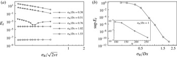
is the estimate of (3.3) from the numerical solution, is plotted in semilogarithmic scale in panel (a) of figure 3 for different spatial resolutions, namely the ratio
 ${\it\sigma}_{R}/Dx$
versus
 ${\it\sigma}_{R}/\ell _{0}(t)$
, which in this case serves as dimensionless time
 $\sqrt{{\it\epsilon}_{R}/t}$
. In the unresolved cases (
 ${\it\sigma}_{R}/Dx<1$
), the error is order one and increases in time. In contrast, when a proper spatial resolution is adopted, i.e.
 ${\it\sigma}_{R}/Dx>1$
, the error becomes progressively smaller as the resolution is increased and stays constant in time. In other words, as the simulation advances in time
 $E_{I}$
does not accumulate. Panel (b) of figure 3 reports the supreme
 $\sup _{t\geqslant 0}E_{I}$
as a function of the ratio
 ${\it\sigma}_{R}/Dx$
. This plot emphasizes the convergence rate of the impulse against the spatial resolution. The inset shows
 $\sup _{t\geqslant 0}E_{I}$
in a different manner. Here, the ratio
 ${\it\sigma}_{R}/Dx$
is fixed to one, and the number of grid points
 $N$
in each direction is progressively increased, denoting convergence also with respect to the grid refinement.
Convergence study in the case of a constant force
 $\boldsymbol{F}=(F_{0},0,0)$
applied at a fixed point
 $\boldsymbol{x}_{p}$
to the fluid initially at rest in a periodic box
 $\mathscr{D}$
. (a) The error
 $E_{I}$
of the total impulse is plotted for different values of the spatial resolution
 ${\it\sigma}_{R}/Dx$
against the dimensionless parameter
 ${\it\sigma}_{R}/\sqrt{2{\it\nu}t}$
, which serves as dimensionless time
 $\sqrt{{\it\epsilon}_{R}/t}$
. (b) The supreme
 $\sup _{t\geqslant 0}E_{I}$
is plotted against the ratio
 ${\it\sigma}_{R}/Dx$
. The inset reports the supreme
 $\sup _{t\geqslant 0}E_{I}$
against the number of grid points
 $N$
for a fixed spatial resolution
 ${\it\sigma}_{R}/Dx=1$
.

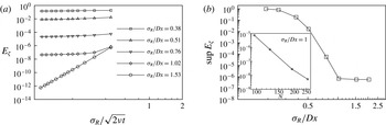
The impulse, although a fundamental quantity, does not retain any information concerning the spatial structure of the fluid field. To go into more depth in the convergence analysis we have addressed the vorticity field. The error is now defined by using the standard
 $L^{2}$
norm as
 $E_{{\bf\zeta}}=\Vert {\bf\zeta}_{E}-{\bf\zeta}_{N}\Vert _{2}/\Vert {\bf\zeta}_{E}\Vert _{2}$
, where the subscripts refer to the exact solution and its numerical counterpart (2.17). The error
 $E_{{\bf\zeta}}$
is shown in panel (a) of figure 4 for different spatial resolutions, namely the ratio
 ${\it\sigma}_{R}/Dx$
versus
 ${\it\sigma}_{R}/\ell _{0}(t)$
. When a proper spatial resolution is adopted, the error
 $E_{{\bf\zeta}}$
also stays constant in time or decreases. It should be noted that the largest error is achieved at the early stages of the simulation when the force is applied to the fluid at rest. In any case, the supreme
 $\sup _{t\geqslant 0}E_{{\bf\zeta}}$
converges when the spatial resolution is progressively refined, as shown in panel (b) of the figure. The inset reports
 $\sup _{t\geqslant 0}E_{{\bf\zeta}}$
against the number of grid points
 $N$
, documenting the convergence of
 $\sup _{t\geqslant 0}E_{{\bf\zeta}}$
also with respect to the grid resolution.
Convergence study in the case of a constant force
 $\boldsymbol{F}=(F_{0},0,0)$
applied at a fixed point
 $\boldsymbol{x}_{p}$
to the fluid initially at rest in a periodic box
 $\mathscr{D}$
. (a) The error
 $E_{{\bf\zeta}}$
, see text for definition, is plotted against
 ${\it\sigma}_{R}/\sqrt{2{\it\nu}t}$
for different values of the spatial resolution
 ${\it\sigma}_{R}/Dx$
. (b) The supreme
 $\sup _{t\geqslant 0}E_{{\bf\zeta}}$
is shown as a function of the ratio
 ${\it\sigma}_{R}/Dx$
. The inset reports the supreme
 $\sup _{t\geqslant 0}E_{{\bf\zeta}}$
versus the grid points
 $N$
for a fixed spatial resolution
 ${\it\sigma}_{R}/Dx=1$
.

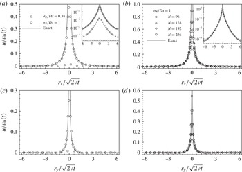
More detailed insight concerning the ensuing fluid motion generated by the fixed force is achieved by a direct inspection of the flow field. Panels (a) and (b) of figure 5 report the velocity disturbance
 $u/u_{0}$
in the direction of the force as a function of
 $r_{x}/\ell _{0}$
in a one-dimensional cut through the point where the force is applied. The curves in the plot pertain to simulations that have different spatial resolutions. Namely, a typical unresolved case
 ${\it\sigma}_{R}/Dx=0.38$
and a resolved simulation
 ${\it\sigma}_{R}/Dx=1$
are compared against the exact solution given by (3.1) in self-similar variables. As shown in the plot, when
 ${\it\sigma}_{R}/Dx\geqslant 1$
the present algorithm reproduces the exact solution well. It should be noted that insufficient spatial resolution results in a clear underestimate of the fluid velocity disturbance. This is emphasized by the curves reported in the inset, where the data are represented in a semilogarithmic scale. Panel (b) of figure 5 documents the behaviour of the ERPP method when the spatial resolution
 ${\it\sigma}_{R}/Dx$
is kept fixed and the regularization length scale
 ${\it\sigma}_{R}$
is progressively reduced, i.e. the grid resolution
 $N$
is progressively increased. In fact, as
 ${\it\sigma}_{R}$
is decreased, the numerical solution describes a progressively wider range of the exact solution, avoiding in all cases the occurrence of the singularity at the point
 $\boldsymbol{x}_{p}$
where the force is applied,
 $r_{x}=0$
in the plot. The different cases share the same far-field behaviour away from
 $\boldsymbol{x}_{p}$
irrespective of the value of
 ${\it\sigma}_{R}$
, as emphasized by the plots in the insets of figure 5 where the velocity disturbance is represented in a semilogarithmic scale. In summary, the solution provided by ERPP retains the relevant features of the exact solution and avoids the occurrence of the singularity at
 $\boldsymbol{x}_{p}$
, which is clearly an unwanted trait in any numerical solution. Panels (c) and (d) of figure 5 reinforce the conclusion of the previous analysis by showing the fluid velocity component in the direction of the force
 $u$
as a function of the distance
 $r_{y}$
in a transverse one-dimensional cut through the point of application of the force in comparison with the exact solution given by (3.2).
Fluid velocity disturbance generated by a fixed constant force
 $\boldsymbol{F}_{0}=(F_{0},0,0)$
on an initially motionless fluid. The
 $1D$
normalized fluid velocity profile
 $u/u_{0}$
in the direction of the force is plotted against the separation
 $r_{x}/\ell _{0}$
(a and b) and
 $r_{y}/\ell _{0}$
(c and d). The exact solutions (3.1) and (3.2) are reported for comparison in (a,b) and (c,d) respectively (solid line). In (a) and (c)
 $u/u_{0}$
is plotted versus separation for two spatial resolutions, namely
 ${\it\sigma}_{R}/Dx=0.38$
(▫) and
 ${\it\sigma}_{R}/Dx=1$
(○). In (b) and (d)
 $u/u_{0}$
is plotted versus separation for several values of the grid resolution
 $N$
, namely
 $N=96$
(▫),
 $N=128$
(▵),
 $N=192$
(♢) and
 $N=256$
(○), at a fixed ratio
 ${\it\sigma}_{R}/Dx=1$
. The insets of (a) and (b) show the data in a semilogarithmic scale.

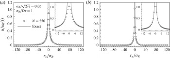
Finally, figure 6 reports the fluid velocity disturbance
 $u/u_{0}$
plotted against the normalized distances
 $r_{x}/{\it\sigma}_{R}$
and
 $r_{y}/{\it\sigma}_{R}$
. The discussion of these plots requires some care. The ERPP model was conceived to describe the far-field effect produced on the fluid by a point-like particle, avoiding the occurrence of singularities at the point
 $\boldsymbol{x}_{p}$
where the particle is located. In fact, the disturbance produced by the particle is described by retaining only the first term in the multipole expansion of the general solution of the unsteady Stokes flow, and the regularization time scale
 ${\it\epsilon}_{R}$
accounts for the viscous diffusion process which naturally regularizes the solution. Hence, the solution provided by ERPP has an intrinsic inner cutoff provided by
 ${\it\sigma}_{R}$
and is expected to reproduce the disturbance flow generated by a point particle in the far field. This is indeed what happens and what is documented by the plots in figure 6. The regularized solution stays on top of the exact solution everywhere, see e.g. the main panels of figure 6 which, on the scale of the complete computational domain
 $\mathscr{D}$
, report the fluid velocity disturbance produced by the particle. The insets of figure 6 show the same data in the proximity of the origin where the particle is placed. This representation emphasizes that, after a distance of a few
 ${\it\sigma}_{R}$
, the ERPP solution falls on top of the exact solution. The threshold
 $3{\it\sigma}_{R}$
can be safely assumed as an inner cutoff for the disturbance flow field produced by the particle.
Fluid velocity disturbance generated by a fixed constant force
 $\boldsymbol{F}_{0}=(F_{0},0,0)$
on an initially motionless fluid. The 1D normalized fluid velocity profile
 $u/u_{0}$
in the direction of the force is plotted against the separation
 $r_{x}/{\it\sigma}_{R}$
(a) and
 $r_{y}/{\it\sigma}_{R}$
(b) at
 ${\it\sigma}_{R}/\sqrt{2{\it\nu}t}=0.05$
for a given spatial resolution of
 $N=256$
grid points and
 ${\it\sigma}_{R}/Dx=1$
. The exact solutions (3.1) and (3.2) are also reported for comparison (solid line). The insets of (a) and (b) provide a close-up view of the solution at
 $\boldsymbol{x}_{p}=0$
.

3.2. Unsteady motion of an isolated particle
The following subsections address more realistic cases where the point
 $\boldsymbol{x}_{p}$
is allowed to move according to (2.39) with the initial conditions
 $\boldsymbol{x}_{p}(t=0)=\boldsymbol{x}_{p}^{0},\boldsymbol{v}_{p}(t=0)=0$
. In order to proceed gradually, we will first discuss a series of tests where the particle motion is not affected by the fluid velocity disturbance that the particle generates. In such decoupled cases the fluid disturbance field is still amenable to exact solutions which can be employed for further comparisons. Subsequently, we will consider the fully coupled case where the dynamics of the particles and the fluid are intertwined.
3.2.1. Imposed particle motion
We consider the motion of a small particle subjected to an external force, e.g. gravity, and to the Stokes drag. The particle velocity is given by the solution of the equation
 $$\begin{eqnarray}m_{p}\frac{\text{d}\boldsymbol{v}_{p}}{\text{d}t}=m_{p}\boldsymbol{g}-6{\rm\pi}{\it\mu}a_{p}\boldsymbol{v}_{p}(t),\end{eqnarray}$$
namely
 $$\begin{eqnarray}v_{p}(t)=v_{t}(1-\text{e}^{-t/{\it\tau}_{p}}),\end{eqnarray}$$
where
 $v_{p}(t)$
denotes the particle velocity in the direction of the gravity acceleration, say the
 $x$
direction,
 $v_{t}={\it\tau}_{p}\,g$
is the particle terminal velocity and
 ${\it\tau}_{p}={\it\rho}_{p}d_{p}^{2}/18{\it\mu}$
is the Stokes relaxation time scale. In this framework the motion of the particle is imposed and its dynamics is decoupled from the dynamics of the carrier fluid.
Panel (a) of figure 7 reports the fluid velocity disturbance produced by the moving particle at
 $t/{\it\tau}_{p}=20$
when the particle has reached its terminal velocity
 $v_{t}$
. The fluid velocity profile is plotted for two cases which differ in the value of the regularization length scale
 ${\it\sigma}_{R}$
for
 ${\it\sigma}_{R}/Dx=1$
. Once again the value of
 ${\it\sigma}_{R}$
controls the regularized near field and does not affect the far field, see the inset of the figure. In the case of the moving particle the fluid velocity also has an explicit solution given by the time convolution integral of the unsteady Stokeslet, (A 13), and the hydrodynamic force
 $D_{p}(t)$
where the Stokeslet is placed at the instantaneous particle position as specified by (3.5). It is now a little more tricky to perform the time convolution integral than in the example discussed in § 3.1 since
 $\boldsymbol{r}=\boldsymbol{x}-\boldsymbol{x}_{p}(t)$
where
 ${\dot{x}}_{p}=v_{p}(t)$
. In fact, the integration of the expression
 $$\begin{eqnarray}u_{i}(\boldsymbol{r},t)=\int _{0}^{t}\unicode[STIX]{x1D60E}_{ik}[\boldsymbol{x}-\boldsymbol{x}_{p}({\it\tau}),t-{\it\tau}]D_{k}^{p}({\it\tau})\,\text{d}{\it\tau}\end{eqnarray}$$
in a closed form becomes cumbersome even though the integral can be evaluated numerically by a quadrature formula. Indeed, such numerical approximation of the exact solution can be still used for useful comparisons. The data produced by the ERPP algorithm are compared with the reference solution (3.6) in figure 7. The plots show that the ERPP approach is able to capture the expected solution and provides a consistent regularization of the singularity that occurs at
 $\boldsymbol{x}_{p}$
. Panel (b) of figure 7 provides the fluid velocity disturbance produced by particles with different terminal velocities
 $v_{t}$
. The effect of increasing the terminal velocity is worth discussing. As
 $v_{t}$
is increased the fore–aft symmetry in the disturbance flow is progressively broken. This symmetry breaking is indeed easily explained in terms of vorticity released along the path of the moving particle. In fact, in the body-fixed frame, the convective term
 $\boldsymbol{v}_{p}\boldsymbol{\cdot }\boldsymbol{{\rm\nabla}}\boldsymbol{u}$
is responsible of the constant velocity advection for the vorticity even in a Stokes regime.
Normalized fluid velocity disturbance produced by a particle moving with velocity
 $v_{p}(t)=v_{t}(1-\text{e}^{-t/{\it\tau}_{p}})$
in the
 $x$
direction in a periodic box
 $\mathscr{D}$
. The normalized velocity disturbance
 $u/v_{t}$
in the direction of the particle motion is plotted against the separation
 $r_{x}/a_{p}$
at time
 $t/{\it\tau}_{p}=20$
when the particle has reached the terminal velocity
 $v_{t}$
. (a) Data obtained for different values of the regularization length scale
 ${\it\sigma}_{R}$
at a fixed spatial resolution
 ${\it\sigma}_{R}/Dx=1$
, namely
 $N=192$
(▵) and
 $N=384$
(○), are compared against the exact solution (solid line) given by (3.6). The inset reports the data of the main panel plotted in a semilogarithmic scale. (b) Data pertaining to particles with different terminal velocities, namely
 $v_{t}^{\ast }=v_{t}d_{p}/{\it\nu}=10^{-5}$
(▫) and
 $v_{t}^{\ast }=10^{-3}$
(○), are compared against the corresponding exact solution (3.6), shown by the dashed and solid line respectively. The inset reports the data of the main panel plotted in a semilogarithmic scale.

We conclude the discussion by presenting in figure 8 the comparison between the ERPP solution and what one would obtain by using the classical PIC approach. As expected, the solution provided by the PIC method is grid dependent, as demonstrated by comparing the disturbance velocity profiles of two simulations that share the same physical parameters but differ in the grid resolution, namely
 $N=192$
and
 $N=384$
grid points. As the grid is refined, a singular-like behaviour occurs at
 $\boldsymbol{x}_{p}$
and the field is characterized by numerical aliasing, see e.g. inset (b) where the velocity profile is plotted in a semilogarithmic scale. In contrast, once the regularization time scale
 ${\it\epsilon}_{R}$
(or equivalently the length scale
 ${\it\sigma}_{R}$
) is fixed, the ERPP approach provides a numerically convergent asymptotically grid-independent solution. This behaviour can be better appreciated in inset (a) where a close-up view of the velocity disturbance is reported. In a nutshell, ERPP retains all the features of the physical solution produced by a small point-like particle except for the (undesired) singularity which unavoidably occurs at
 $\boldsymbol{x}_{p}$
. The regularization of the solution is controlled by the time scale
 ${\it\epsilon}_{R}$
which is related to a diffusive length scale
 ${\it\sigma}_{R}$
. Indeed,
 ${\it\sigma}_{R}$
is naturally introduced by the process of vorticity diffusion and can be fixed on a physical ground. For instance, in a turbulent flow, velocity fluctuations are physically irrelevant below the Kolmogorov length scale
 ${\it\eta}$
. At the same time the effects that a swarm of point-like particles generate on length scales larger than
 ${\it\eta}$
are physically relevant. In such a framework the regularization length scale
 ${\it\sigma}_{R}$
is naturally selected as
 ${\it\sigma}_{R}={\it\eta}$
.
Normalized fluid velocity disturbance at
 $t/{\it\tau}_{p}=20$
produced by a particle moving with velocity
 $v_{p}(t)=v_{t}(1-\text{e}^{-t/{\it\tau}_{p}})$
in the
 $x$
direction. The velocity profile ensuing from ERPP for different values of the regularization length scale
 ${\it\sigma}_{R}$
and grid resolution, namely
 $N=192$
,
 ${\it\sigma}_{R}/Dx=1$
(▫),
 $N=384$
,
 ${\it\sigma}_{R}/Dx=2$
(▵) and
 $N=384$
,
 ${\it\sigma}_{R}/Dx=1$
(○), is compared against the exact solution given by (3.6) (solid red line) and the corresponding results obtained by the PIC approach, namely
 $N=192$
(▿) and
 $N=384$
(♢). Inset (a) shows a close-up view of the velocity disturbance near the singular point
 $\boldsymbol{x}_{p}$
. Inset (b) shows the velocity profile plotted in a semilogarithmic scale.

3.2.2. Particle motion in the coupled regime
This subsection addresses the unsteady motion of a particle that settles from rest under the action of gravity in the coupled regime where the particle induces a disturbance in the surrounding fluid and this disturbance enters the expression of the hydrodynamic force. For simplicity we will consider small particles much heavier than the surrounding fluid, i.e.
 ${\it\rho}_{p}\gg {\it\rho}_{f}$
, where the only relevant force is the Stokes drag. The general expression of the force (2.40) simplifies to
 $$\begin{eqnarray}\boldsymbol{D}_{p}(t)=m_{p}\boldsymbol{g}+6{\rm\pi}{\it\mu}a_{p}[\tilde{\boldsymbol{u}}(\boldsymbol{x}_{p},t)-\boldsymbol{v}_{p}(t)].\end{eqnarray}$$
Following the discussion of § 2.5 the velocity
 $\tilde{\boldsymbol{u}}(\boldsymbol{x}_{p},t)$
must be interpreted as the background fluid velocity in the absence of the
 $p$
th particle, e.g. turbulent fluctuations plus the disturbance flow generated by all the other particles. This makes the calculation of the hydrodynamic force particularly challenging in the two-way coupling regime. In the particular case where only one particle is considered the value
 $\tilde{\boldsymbol{u}}(\boldsymbol{x}_{p},t)$
should be set to zero. However this way of proceeding is unfeasible in the general case where many particles are present since the value of
 $\tilde{\boldsymbol{u}}(\boldsymbol{x}_{p},t)$
must also account for the velocity disturbance generated by all the other particles and the background flow. This conundrum can be disentangled in the context of the ERPP approach since the disturbance flow produced by the
 $p$
th particle on itself is known in a closed form and thus can be removed from the background fluid velocity
 $\boldsymbol{u}(\boldsymbol{x}_{p},t)$
even in the presence of many other particles.
The two panels of figure 9 provide evidence on the above considerations. The plots report the particle velocity normalized with the settling velocity
 $v_{t}$
as a function of the dimensionless time
 $t/{\it\tau}_{p}$
both for the ERPP calculation and for the PIC approach. The particle trajectory should be compared with the reference solution given by (3.5). Panel (a) shows the particle velocity calculated by the ERPP method for different values of the ratio
 $d_{p}/{\it\sigma}_{R}$
. We recall that our approach is designed to model the disturbance flow produced by point-like particles, i.e. particles whose diameter
 $d_{p}$
is much smaller that any other length scale in the system. In the ERPP approach, in the absence of any other length scales introduced by the background flow, the only significant length scale is the diffusive scale
 ${\it\sigma}_{R}$
. Hence, the nominal diameter of the particle should be smaller than
 ${\it\sigma}_{R}$
. Indeed, as the ratio
 $d_{p}/{\it\sigma}_{R}$
decreases the particle velocity rapidly approaches the reference curve provided by (3.5). When the scale
 ${\it\sigma}_{R}$
has been fixed ERPP gives a grid-independent solution, as can be appreciated in figure 9 where two trajectories that share the same
 ${\it\sigma}_{R}$
but have different grids, namely
 $N=192$
and
 $N=24$
grid points in each direction, give practically undistinguishable results. It is worth noting that the error in the particle velocity is already below 10 % for the relatively large ratio
 $d_{p}/{\it\sigma}_{R}=0.5$
we have considered. Panel (b) of figure 9 reports the particle velocity calculated with the PIC method. The solution now presents larger deviations from the exact result (3.5). This is due to a poor estimate of the hydrodynamic force. In fact, in the PIC approach the self-induced disturbance produced by the
 $p$
th particle is unknown or, if eventually modelled by the steady Stokeslet, is singular at the particle position
 $\boldsymbol{x}_{p}$
. In both cases it cannot be removed from the particle-to-fluid slip velocity, resulting in an inaccurate prediction of the hydrodynamic force and, consequently, of the particle trajectory. For instance, for
 $d_{p}/Dx=0.5$
the error in the terminal velocity is 50 % for the PIC approach compared with a much lower 10 % for ERPP. Clearly, the error reduces as the ratio
 $d_{p}/Dx\rightarrow 0$
.
Normalized particle velocity
 $v_{p}/v_{t}$
as a function of the dimensionless time
 $t/{\it\tau}_{p}$
. (a) Particle velocity in the ERPP simulations for different values of the ratio
 $d_{p}/{\it\sigma}_{R}$
, namely
 $d_{p}/{\it\sigma}_{R}=0.5$
(▫),
 $d_{p}/{\it\sigma}_{R}=0.25$
(▵),
 $d_{p}/{\it\sigma}_{R}=0.125$
(♢) and
 $d_{p}/{\it\sigma}_{R}=0.0625$
(○). The fluid field is resolved with
 $N=192$
grid points (Fourier modes) for each direction (open symbols) in a periodic box
 $L_{B}=2{\rm\pi}$
. In the case
 $d_{p}/{\it\sigma}_{R}=0.0625$
(▪) the fluid field is resolved with
 $N=24$
grid points (in each direction) to check grid independence. (b) Particle velocity provided by the PIC approach in comparable conditions to ERPP. Here,
 $d_{p}/Dx=0.5$
(▫),
 $d_{p}/Dx=0.25$
(▵),
 $d_{p}/Dx=0.125$
(♢) and
 $d_{p}/Dx=0.0625$
(○). In (a) and (b) the reference solution (3.5) is reported for comparison (solid line).

A more direct comparison between the two approaches is provided in panel (a) of figure 10 where we plot the particle velocity for the largest ratio
 $d_{p}/{\it\sigma}_{R}=0.5$
and the smallest one
 $d_{p}/{\it\sigma}_{R}=0.0625$
for both ERPP and PIC. For comparison, in the ERPP calculation we have reported the particle velocity in a case where we did not subtract from
 $\boldsymbol{u}(\boldsymbol{x}_{p},t)$
the self-induced disturbance. Panel (b) of the figure presents the relative error in the estimate of the terminal velocity as a function of
 $d_{p}/{\it\sigma}_{R}$
. Although the error scaling with grid resolution is comparable (see inset), the error pertaining to the ERPP approach is substantially smaller. A last issue concerns the sensitivity of the ERPP method in poorly resolved cases where
 ${\it\sigma}_{R}/Dx<1$
. In figure 11 we compare the particle velocity for three different resolutions at fixed
 $d_{p}/{\it\sigma}_{R}$
. As expected, the method loses accuracy as the regularization kernel is not resolved on the computational grid.
Normalized particle velocity
 $v_{p}/v_{t}$
as a function of the dimensionless time
 $t/{\it\tau}_{p}$
. (a) Direct comparison of the ERPP results against the PIC approach and the reference solution (solid line) for different values of the ratio
 $d_{p}/{\it\sigma}_{R}$
or equivalently
 $d_{p}/Dx$
, namely
 $d_{p}/{\it\sigma}_{R}{-}d_{p}/Dx=0.5$
(squares) and
 $d_{p}/{\it\sigma}_{R}{-}d_{p}/Dx=0.0625$
(circles). Black filled symbols refer to the PIC approach, open symbols to the ERPP method. The grey square refers to an ERPP calculation where intentionally we did not remove the self-induced velocity disturbance. (b) Relative error in the evaluation of the terminal velocity as a function of the dimensionless parameter
 $d_{p}^{\ast }=d_{p}/{\it\sigma}_{R}$
for ERPP and PIC. The inset shows the data plotted on a log–log scale.

Normalized particle velocity
 $v_{p}/v_{t}$
as a function of the dimensionless time
 $t/{\it\tau}_{p}$
. The trajectories obtained in two unresolved cases, namely
 ${\it\sigma}_{R}/Dx=0.5$
and
 ${\it\sigma}_{R}/Dx=0.25$
, are compared against a resolved case at
 ${\it\sigma}_{R}/Dx=1$
for a given value of the ratio
 $d_{p}/{\it\sigma}_{R}=0.0625$
.

Additional validation of the approach is discussed in § A.6 by comparison with known solutions for systems of hydrodynamically coupled particles.
4. Application to turbulent flows
In order to discuss the feasibility of turbulent particle-laden flow simulations, in this section we present preliminary results obtained by the ERPP method for a homogeneous shear flow at moderate Reynolds number. The mean velocity profile in the
 $x$
direction (streamwise direction) is imposed and is characterized by a constant velocity gradient
 $S$
along the
 $y$
direction (shear direction). The third coordinate is denoted by
 $z$
(spanwise direction). The Reynolds decomposition
 $\boldsymbol{u}=Sy\boldsymbol{e}_{x}+\boldsymbol{u}^{\prime }$
allows us to write the Navier–Stokes equations for the turbulent fluctuating component
 $\boldsymbol{u}^{\prime }$
, which are solved in a reference frame advected by the mean flow, see e.g. Rogallo (Reference Rogallo1981). Rogallo’s transformation allows us to restore the spatial homogeneity of the fluctuations in the convected frame. A sketch of the flow domain is reported in figure 12.
Sketch of the flow configuration. The flow domain is represented by a periodic box of length
 $L_{x}=4{\rm\pi}$
,
 $L_{y}=2{\rm\pi}$
and
 $L_{z}=2{\rm\pi}$
in the steamwise, shear and spanwise directions respectively. The mean flow
 $Sy\boldsymbol{e}_{x}$
is in the
 $x$
direction and linearly changes at a rate
 $S$
along the
 $y$
direction. The contour plot shows the intensity of the velocity fluctuations in selected coordinate planes.

In the homogeneous shear flow the turbulent fluctuations are sustained by the off-diagonal component of the Reynolds shear stress,
 $-\langle u\,v\rangle$
, resulting in a neat turbulent kinetic energy production rate
 $\mathscr{P}=-S\langle u\,v\rangle$
. The growth of the integral scale is eventually bounded by the computational box, originating a pseudo-cyclic behaviour of the turbulent kinetic energy and the enstrophy, as discussed in Pumir (Reference Pumir1996), Gualtieri et al. (Reference Gualtieri, Casciola, Benzi, Amati and Piva2002) and Yakhot (Reference Yakhot2003). Stationarity must be intended in the sense that the pseudo-cyclic oscillations repeat themselves indefinitely, yielding time-independent ensemble averages, see e.g. the extensive discussion in Gualtieri et al. (Reference Gualtieri, Casciola, Benzi and Piva2007) where most of the relevant literature was reported.
The large-scale anisotropic forcing due to the Reynolds shear stress feeds the energy cascade operated by the nonlinear terms of the Navier–Stokes equations, which eventually restore isotropy at smaller scales. The so-called shear scale
 $L_{S}$
ideally separates the production range
 $L_{S}<\ell <L_{0}$
(
 $L_{0}$
is the integral scale), from the isotropy recovery range
 ${\it\eta}<\ell <L_{S}$
. It follows that the nature of turbulent fluctuations is parametrized by two dimensionless parameters, the shear intensity
 $S^{\ast }=(L_{0}/L_{S})^{2/3}$
and the Corsin parameter
 $S_{c}=({\it\eta}/L_{S})^{2/3}$
. The latter can be recast in terms of the inverse of the classical turbulent Reynolds number
 $Re_{{\it\lambda}}$
based on the Taylor length scale.
In the conditions discussed above the transport of inertial particles is non-trivial. In fact, the disperse phase is characterized by small-scale aggregates (clusters) which preserve a spatial preferential orientation induced by the large-scale motions, up to the smallest scales where, in contrast, turbulent fluctuations recover isotropy, see e.g. Gualtieri, Picano & Casciola (Reference Gualtieri, Picano and Casciola2009) and Gualtieri et al. (Reference Gualtieri, Picano, Sardina and Casciola2013).
The first result concerns a flow at a Taylor-based Reynolds number of
 $\mathit{Re}_{{\it\lambda}}=70$
and shear intensity of
 $S^{\ast }=7$
. The carrier phase is resolved by using
 $N_{x}\times N_{y}\times N_{z}=256\times 256\times 128$
Fourier modes in a
 $4{\rm\pi}\times 2{\rm\pi}\times 2{\rm\pi}$
periodic box. This spectral-based discretization corresponds to
 $384\times 384\times 192$
collocation points in physical space due to the
 $3/2$
dealiasing procedure required for the calculation of the nonlinear terms. The spatial discretization fully resolves the Kolmogorov length scale with
 ${\it\eta}/Dx\sim 1.50$
, and
 ${\it\sigma}_{R}$
is chosen to match
 ${\it\eta}$
. Time integration is performed by the low-storage Runge–Kutta method already mentioned in § 3. The carrier fluid is laden with
 $N_{p}=2200\,000$
inertial particles. The particle-to-fluid density ratio is
 ${\it\rho}_{p}/{\it\rho}_{f}=1800$
, corresponding to a Stokes number
 $\mathit{St}_{{\it\eta}}={\it\tau}_{p}/{\it\tau}_{{\it\eta}}=1$
, where
 ${\it\tau}_{p}=({\it\rho}_{p}/{\it\rho}_{f})d_{p}^{2}/18{\it\nu}$
is the Stokes relaxation time and
 ${\it\tau}_{{\it\eta}}$
is the Kolmogorov time scale. In such conditions the particle diameter
 $d_{p}$
is much smaller than the Kolmogorov length, namely
 $d_{p}/{\it\eta}=0.1$
. The mass load
 ${\it\Phi}$
, defined as the ratio between the masses of the disperse phase and the carrier fluid, is
 ${\it\Phi}=0.4$
.
In figure 13 we present a snapshot of the particle position in an
 $xy$
plane containing the mean flow (from left to right). As expected, particles with unitary Stokes number are characterized by small-scale clusters, i.e. the particles concentrate in narrow regions, clusters, separated by voids where no particles can be found. The preferential alignment of the aggregates along the principal strain direction of the mean flow is also evident from the snapshot. This is the signature of the persistent anisotropy of the clusters at small scales. In the context of the ERPP methodology we are able to compute in a closed form the forcing operated by the particles on the fluid. In figure 13(b) we report the intensity of the forcing term of (2.35) which accounts for the backreaction on the fluid. The pattern of the backreaction field is strongly correlated to the cluster structure and inherits from the latter its characteristic multiscale nature. The forcing is actually active in a broad range of scales up to the smallest scales where intense peaks occur. It should be noted, however, that the forcing field is everywhere smooth and can be successfully represented on the discrete grid by virtue of the regularization naturally operated by the viscosity. The highest forcing intensity is localized in the spatial regions where the particles are concentrated, while in the void regions the forcing vanishes. The correlation between the instantaneous spatial configuration of the particles and the corresponding backreaction on the fluid can be visually appreciated in panel (c) of the figure where the two fields are superimposed.
Snapshot of the instantaneous particle configuration (a) and corresponding intensity of the forcing on the fluid (b) in a thin slice along the
 $xy$
plane. The mean flow
 $S\,y$
is in the
 $x$
direction from left to right. In (c), (a) and (b) are superimposed to provide a visual correlation between the instantaneous particle configuration and the corresponding forcing field.

As anticipated, this short section was aimed at the clear illustration of the potential of ERPP in dealing with actual turbulent flows laden with millions of particles. Clearly, a complete analysis of the turbulence modulation in the two-way coupling regime would require a more complete statistical analysis, which is, however, beyond the scope of the present work and is postponed to future investigation.
5. Final remarks
In this paper we have presented a new methodology, dubbed the ERPP method, able to capture the inter-phase momentum exchange between a carrier flow and a disperse phase modelled as lumped massive points. The coupling mechanism is designed on the physical grounds provided by the unsteady Stokes flow around a small sphere. In short, along its trajectory the particle continuously generates a highly localized vorticity field that can be evaluated in a closed form. Successively, because of viscous diffusion, the vorticity field reaches the physically significant length scales of the flow field. When this occurs, the newly generated vorticity can be injected into the computational grid where the Navier–Stokes equations for the carrier flow are solved, thus achieving the inter-phase momentum coupling. In this approach the viscous diffusion naturally regularizes the disturbance flow produced by each particle without requiring any ‘ad hoc’ numerical artefact. The proposed approach can be implemented in a highly efficient computational algorithm since the disturbance produced by a particle is strongly compact in space and is localized around the actual particle position. This means that at each time step only few grid points perceive the particle disturbance which decays exponentially fast in space. As a consequence, the ERPP method can handle millions of particles at an affordable computational cost, as proved by preliminary results for a particle-laden turbulent homogeneous shear flow in the two-way coupling regime.
The ERPP method overcomes several drawbacks of established methods, like the PIC method. Indeed, the regularization of the backreaction field provided by the viscous diffusion allows numerically convergent solutions, preventing the strong grid dependence which spoils singularity-based approximations. Even more importantly, the ERPP method solves the intrinsic difficulty of numerical simulations in the two-way coupling regime associated with the calculation of the correct particle-to-fluid slip velocity. Actually, in the ERPP method the disturbance flow produced by the particles at each time step can be evaluated in a closed form. This allows the spurious self-induced velocity disturbance to be removed from the particle-to-fluid slip velocity, allowing for a correct evaluation of the hydrodynamic force.
The preliminary results concerning a turbulent particle-laden shear flow presented in § 4 demonstrate the potential of the ERPP method in the simulation of turbulent flows in the two-way coupling regime. It is known that the dynamics of the two-phase system is fully characterized by a given set of dimensionless parameters, namely
 $\{\mathit{Re}_{0},\,\mathit{St}_{{\it\eta}},\,{\it\rho}_{p}/{\it\rho}_{f},\,d_{p}/{\it\eta},\,{\it\Phi},\,N_{p}\}$
. To comment on the effectiveness of the ERPP method in modelling turbulent suspensions, let us assume that the turbulence characteristics are prescribed, i.e. the turbulent Reynolds number
 $\mathit{Re}_{0}$
, the integral scale
 $L_{0}$
, the Kolmogorov scale
 ${\it\eta}$
or time scale
 ${\it\tau}_{{\it\eta}}$
are fixed, and let us consider small particles, i.e.
 $d_{p}/{\it\eta}\ll 1$
. In these conditions the Stokes number
 $\mathit{St}_{{\it\eta}}={\it\tau}_{p}/{\it\tau}_{{\it\eta}}$
controls the dynamics of the disperse phase in terms of its preferential spatial accumulation, either small-scale clustering in homogeneous flows (Reade & Collins Reference Reade and Collins2000; Toschi & Bodenschatz Reference Toschi and Bodenschatz2009; Bec et al.
Reference Bec, Biferale, Cencini, Lanotte and Toschi2010; Monchaux, Bourgoin & Cartellier Reference Monchaux, Bourgoin and Cartellier2010; Meneguz & Reeks Reference Meneguz and Reeks2011) or turbophoresis in wall-bounded flows (Marchioli & Soldati Reference Marchioli and Soldati2002; Picano, Sardina & Casciola Reference Picano, Sardina and Casciola2009). Once the Stokes number is fixed, the mass load
 ${\it\Phi}$
follows as
 $$\begin{eqnarray}{\it\Phi}=\frac{{\rm\pi}}{6}\,N_{p}\,\frac{(18\,\mathit{St}_{{\it\eta}})^{3/2}}{({\it\rho}_{p}/{\it\rho}_{f})^{1/2}\,\mathit{Re}_{0}^{9/4}}.\end{eqnarray}$$
The value of
 ${\it\Phi}$
can be adjusted by means of the density ratio
 ${\it\rho}_{p}/{\it\rho}_{f}$
and the number of particles
 $N_{p}$
. However, in an actual experiment the ratio
 ${\it\rho}_{p}/{\it\rho}_{f}$
must fall in the range of the available materials, and the most straightforward way to achieve the desired mass load consists in adjusting the number of particles
 $N_{p}$
. Although rather easy in experiments, adjustment of the number of particles turns out to be a big issue in numerical simulations since, most often, the momentum coupling model is unable to handle an arbitrary number of particles while providing grid-independent and physically consistent results. At variance with most available methods, both these requirements are fulfilled by the ERPP approach. Indeed, the number of particles can be freely changed since the disturbance flow and backreaction of each particle are smooth fields. This implies that the solution is correctly reproduced also in flow regions where the particles are extremely dilute, as occurs for the exterior region of turbulent jets or spatially evolving boundary layers. For comparison, classical approaches like the PIC method intrinsically suffer from spurious numerical oscillations in the backreaction field when too few particles per computational cell are available, leading to strong limitations in the achievable mass load
 ${\it\Phi}$
. Indeed, in any direct numerical simulation of a turbulent flow the number of computational cells scales with the Reynolds number as
 $N_{c}\sim \mathit{Re}_{0}^{9/4}$
, suggesting through (5.1) that no room is available to adjust the mass load if the additional constraint
 $N_{p}/N_{c}\sim 1$
needs to be enforced. This limitation is overcome in the approach proposed here by relaxing the requirement on the particle density to allow for the modelling freedom needed to reproduce any physically relevant condition.
Acknowledgements
The research leading to these results has received funding from the European Research Council under the European Union’s Seventh Framework Programme (FP7/2007–2013)/ERC grant agreement no. [339446]. Part of the results of this research have been achieved using the PRACE-2IP project (FP7 RI-283493) resource Zeus based in Poland at Krakow. The authors are grateful to the COST Action MP0806 ‘Particles in Turbulence’ and to PRACE for awarding access to the resource FERMI based in Italy at Casalecchio di Reno.
Appendix A
A.1. Fundamental solution of the diffusion equation
The fundamental solution of the diffusion equation
 $g(\boldsymbol{x}-{\bf\xi},t-{\it\tau})$
can be found by solving the following singularly forced diffusion problem:
 $$\begin{eqnarray}\frac{\partial g}{\partial t}-{\it\nu}{\rm\nabla}^{2}g={\it\delta}(\boldsymbol{x}-{\bf\xi}){\it\delta}(t-{\it\tau}),\end{eqnarray}$$
with
 $\lim _{t\rightarrow {\it\tau}^{-}}g(\boldsymbol{x}-{\bf\xi},t-{\it\tau})=g(\boldsymbol{x}-{\bf\xi},0^{-})=0$
expressing the causality principle. By integrating (A 1) in the interval
 $[{\it\tau}-{\it\epsilon},{\it\tau}+{\it\epsilon}]$
and letting
 ${\it\epsilon}$
approach zero, the singularly forced diffusion equation is recast into an initial-value problem:
 $$\begin{eqnarray}\left.\begin{array}{@{}c@{}}\displaystyle \frac{\partial g}{\partial t}-{\it\nu}{\rm\nabla}^{2}g=0\quad t>{\it\tau},\\ \displaystyle \lim _{t\rightarrow {\it\tau}^{+}}g(\boldsymbol{x}-{\bf\xi},t-{\it\tau})=g(\boldsymbol{x}-{\bf\xi},0^{+})={\it\delta}(\boldsymbol{x}-{\bf\xi}),\end{array}\right\}\end{eqnarray}$$
whose solution is immediate in Fourier space. By denoting with
 ${\hat{g}}(\boldsymbol{k},t-{\it\tau})$
the Fourier transform of
 $g(\boldsymbol{x}-{\bf\xi},t-{\it\tau})$
, (A 2) reads
 $$\begin{eqnarray}\left.\begin{array}{@{}c@{}}\displaystyle \frac{\partial {\hat{g}}}{\partial t}+{\it\nu}\Vert \boldsymbol{k}\Vert ^{2}{\hat{g}}=0\quad t>{\it\tau},\\ \displaystyle \lim _{t\rightarrow {\it\tau}^{+}}{\hat{g}}(\boldsymbol{k},t-{\it\tau})={\hat{g}}(\boldsymbol{k},0^{+})=\frac{1}{(2{\rm\pi})^{3}}.\end{array}\right\}\end{eqnarray}$$
The solution in Fourier space is
 $$\begin{eqnarray}{\hat{g}}(\boldsymbol{k},t-{\it\tau})=\frac{1}{(2{\rm\pi})^{3}}\exp [-{\it\nu}\Vert \boldsymbol{k}\Vert ^{2}(t-{\it\tau})],\end{eqnarray}$$
which, after inverse Fourier transformation, yields the fundamental solution
 $$\begin{eqnarray}g(\boldsymbol{x}-{\bf\xi},t-{\it\tau})=\frac{1}{[4{\rm\pi}\,{\it\nu}(t-{\it\tau})]^{3/2}}\exp \left[-\frac{\Vert \boldsymbol{x}-{\bf\xi}\Vert ^{2}}{4{\it\nu}(t-{\it\tau})}\right]\end{eqnarray}$$
as a Gaussian function with time-dependent variance
 ${\it\sigma}(t-{\it\tau})=\sqrt{2{\it\nu}(t-{\it\tau})}$
.
A.2. Fundamental solution of the unsteady Stokes equations
The fundamental solution of the unsteady Stokes operator can be found by solving the singularly forced unsteady Stokes equations, namely
 $$\begin{eqnarray}\left.\begin{array}{@{}c@{}}\boldsymbol{{\rm\nabla}}\boldsymbol{\cdot }\boldsymbol{v}=0,\\ \displaystyle {\it\rho}_{f}\frac{\partial \boldsymbol{v}}{\partial t}=-\boldsymbol{{\rm\nabla}}p+{\it\mu}{\rm\nabla}^{2}\boldsymbol{v}+\hat{\boldsymbol{e}}{\it\delta}(\boldsymbol{x}-{\bf\xi}){\it\delta}(t-{\it\tau}),\\ \displaystyle \lim _{t\rightarrow {\it\tau}^{-}}\boldsymbol{v}(\boldsymbol{x}-{\bf\xi},t-{\it\tau})=\boldsymbol{v}(\boldsymbol{x}-{\bf\xi},0^{-})=0,\end{array}\right\}\end{eqnarray}$$
where the singular forcing
 ${\it\delta}(\boldsymbol{x}-{\bf\xi}){\it\delta}(t-{\it\tau})$
is applied at the point
 $\boldsymbol{x}={\bf\xi}$
at time
 $t={\it\tau}$
along the direction
 $\hat{\boldsymbol{e}}$
. The solution of (A 6) is more easily found in terms of the associated vorticity field
 ${\bf\zeta}=\boldsymbol{{\rm\nabla}}\times \boldsymbol{v}$
. By taking the curl of (A 6) it follows that
 $$\begin{eqnarray}{\it\rho}_{f}\frac{\partial {\bf\zeta}}{\partial t}={\it\mu}{\rm\nabla}^{2}{\bf\zeta}-\hat{\boldsymbol{e}}\times \boldsymbol{{\rm\nabla}}{\it\delta}(\boldsymbol{x}-{\bf\xi}){\it\delta}(t-{\it\tau}),\end{eqnarray}$$
with the corresponding initial condition
 ${\bf\zeta}(\boldsymbol{x}-{\bf\xi},0^{-})=0$
. Equation (A 7) can be recast as the standard scalar diffusion equation (A 1) by the ansatz
 $$\begin{eqnarray}{\bf\zeta}=-\frac{1}{{\it\rho}_{f}}\hat{\boldsymbol{e}}\times \boldsymbol{{\rm\nabla}}g.\end{eqnarray}$$
Equations (A 8) and (A 5) provide the solution of the singularly forced unsteady Stokes problem in terms of vorticity. The solution in terms of velocity can be found by introducing a divergence-free vector potential
 $\boldsymbol{A}$
, namely
 $\boldsymbol{v}=\boldsymbol{{\rm\nabla}}\times \boldsymbol{A}$
and
 ${\rm\nabla}^{2}\boldsymbol{A}=-{\bf\zeta}$
. The Laplace equation for the vector potential can be transformed into a scalar equation by looking for solutions for the vector potential in the form
 $$\begin{eqnarray}\boldsymbol{A}=\frac{1}{{\it\rho}_{f}}\hat{\boldsymbol{e}}\times \boldsymbol{{\rm\nabla}}G,\end{eqnarray}$$
where the scalar function
 $G$
satisfies the standard Laplace equation
 ${\rm\nabla}^{2}G=g$
. The solution for
 $G$
reads
 $$\begin{eqnarray}G=-\frac{1}{4{\rm\pi}r}\text{erf}\left(\frac{r}{\sqrt{4{\it\nu}(t-{\it\tau})}}\right),\end{eqnarray}$$
where
 $r=\Vert \boldsymbol{x}-{\bf\xi}\Vert$
. The velocity field can be readily determined by substituting the expressions (A 9) and (A 10) into
 $\boldsymbol{v}=\boldsymbol{{\rm\nabla}}\times \boldsymbol{A}$
. After some algebra the velocity reads
 $$\begin{eqnarray}\boldsymbol{v}=(g\,\boldsymbol{I}-\boldsymbol{{\rm\nabla}}\otimes \boldsymbol{{\rm\nabla}}G)\boldsymbol{\cdot }\hat{\boldsymbol{e}}.\end{eqnarray}$$
The solution (A 11) is usually written in terms of the Green tensor
 $\unicode[STIX]{x1D60E}_{ik}(\boldsymbol{x}-{\bf\xi},t-{\it\tau})$
. In fact, by using (A 5) and (A 10), (A 11) can be written as
 $$\begin{eqnarray}v_{i}=\unicode[STIX]{x1D60E}_{ik}\,\hat{e}_{k},\end{eqnarray}$$
where the Green tensor is given by the expression
 $$\begin{eqnarray}\unicode[STIX]{x1D60E}_{ik}(\boldsymbol{x}-{\bf\xi},t-{\it\tau})=\frac{1}{{\it\rho}_{f}}\left[\left(1+\frac{{\it\sigma}^{2}}{r^{2}}\right)g+\frac{G}{r^{2}}\right]{\it\delta}_{ik}-\frac{1}{{\it\rho}_{f}}\left[\left(1+\frac{3{\it\sigma}^{2}}{r^{2}}\right)g+\frac{3G}{r^{2}}\right]\frac{r_{i}r_{k}}{r^{2}}.\end{eqnarray}$$
The solution of the singularly forced Stokes problem is completed by the expression of the pressure and of the viscous stresses. The pressure field associated with the original problem (A 6) can be computed by taking the divergence of the momentum equation, namely
 $$\begin{eqnarray}{\rm\nabla}^{2}p=\hat{\boldsymbol{e}}\boldsymbol{\cdot }\boldsymbol{{\rm\nabla}}{\it\delta}(\boldsymbol{x}-{\bf\xi}){\it\delta}(t-{\it\tau}).\end{eqnarray}$$
The Laplace equation for the pressure can be readily solved by the substitution
 $p=\hat{\boldsymbol{e}}\boldsymbol{\cdot }\boldsymbol{{\rm\nabla}}q\,\,{\it\delta}(t-{\it\tau})$
. In fact, the function
 $q$
satisfies the Laplace problem
 ${\rm\nabla}^{2}q={\it\delta}(\boldsymbol{x}-{\bf\xi})$
, i.e.
 $q=-1/(4{\rm\pi}r)$
. The pressure field then follows immediately as
 $$\begin{eqnarray}p=\frac{\hat{\boldsymbol{e}}\boldsymbol{\cdot }\boldsymbol{r}}{4{\rm\pi}r^{3}}{\it\delta}(t-{\it\tau}).\end{eqnarray}$$
The stress tensor associated with the singularly forced unsteady Stokes problem can be computed as
 $$\begin{eqnarray}\unicode[STIX]{x1D61B}_{ij}=-p{\it\delta}_{ij}+{\it\mu}\left(\frac{\partial v_{i}}{\partial x_{j}}+\frac{\partial v_{j}}{\partial x_{i}}\right),\end{eqnarray}$$
where the pressure
 $p$
is given by (A 15) and the velocity
 $\boldsymbol{v}$
by (A 12). Usually, the stress tensor is expressed via a third-rank tensor
 $$\begin{eqnarray}\unicode[STIX]{x1D61B}_{ij}=\unicode[STIX]{x1D61B}_{ijk}\hat{e}_{k},\end{eqnarray}$$
where
 $\unicode[STIX]{x1D61B}_{ijk}$
is the Green stress tensor defined as
 $$\begin{eqnarray}\unicode[STIX]{x1D61B}_{ijk}=-\frac{r_{k}}{4{\rm\pi}r^{3}}{\it\delta}(t-{\it\tau}){\it\delta}_{ij}+{\it\mu}\left(\frac{\partial \unicode[STIX]{x1D60E}_{ik}}{\partial x_{j}}+\frac{\partial G_{jk}}{\partial x_{i}}\right).\end{eqnarray}$$
The expression for the Green tensor (A 13) can be substituted into the definition (A 18), and, after some algebra, the final expression for
 $\unicode[STIX]{x1D61B}_{ijk}$
reads
 $$\begin{eqnarray}\displaystyle \unicode[STIX]{x1D61B}_{ijk} & = & \displaystyle -\frac{r_{k}}{4{\rm\pi}r^{3}}{\it\delta}(t-{\it\tau}){\it\delta}_{ij}\nonumber\\ \displaystyle & & \displaystyle +\,{\it\nu}\left[-2\frac{B}{r^{2}}{\it\delta}_{ij}r_{k}+\left(\frac{1}{r}\frac{\text{d}A}{\text{d}r}-\frac{B}{r^{2}}\right)({\it\delta}_{jk}r_{i}+{\it\delta}_{ik}r_{j})-2\left(\frac{2}{r}B+\frac{\text{d}B}{\text{d}r}\right)\frac{r_{i}r_{j}r_{k}}{r^{3}}\right],\qquad\end{eqnarray}$$
where the functions
 $A(r)$
and
 $B(r)$
are defined as
 $$\begin{eqnarray}\left.\begin{array}{@{}c@{}}\displaystyle A(r)=\left(1+\frac{{\it\sigma}^{2}}{r^{2}}\right)g+\frac{G}{r^{2}},\\ \displaystyle B(r)=\left(1+\frac{3{\it\sigma}^{2}}{r^{2}}\right)g+\frac{3}{r^{2}}G.\end{array}\right\}\end{eqnarray}$$
A.3. Evolution of the regular vorticity field, proof of (2.22)
Let us first differentiate (2.17) with respect to time,
 $$\begin{eqnarray}\displaystyle \frac{\partial {\bf\zeta}_{R}}{\partial t} & = & \displaystyle \frac{1}{{\it\rho}_{f}}\boldsymbol{D}_{p}(t-{\it\epsilon}_{R})\times \boldsymbol{{\rm\nabla}}_{x}g[\boldsymbol{x}-\boldsymbol{x}_{p}(t-{\it\epsilon}_{R}),{\it\epsilon}_{R}]\nonumber\\ \displaystyle & & \displaystyle +\,\frac{1}{{\it\rho}_{f}}\int _{0}^{t-{\it\epsilon}_{R}}\boldsymbol{D}_{p}({\it\tau})\times \boldsymbol{{\rm\nabla}}_{x}\frac{\partial g}{\partial t}[\boldsymbol{x}-\boldsymbol{x}_{p}({\it\tau}),t-{\it\tau}]\,\text{d}{\it\tau},\end{eqnarray}$$
take the Laplacian,
 $$\begin{eqnarray}{\rm\nabla}^{2}{\bf\zeta}_{R}=\frac{1}{{\it\rho}_{f}}\int _{0}^{t-{\it\epsilon}_{R}}\boldsymbol{D}_{p}({\it\tau})\times \boldsymbol{{\rm\nabla}}_{x}{\rm\nabla}^{2}g[\boldsymbol{x}-\boldsymbol{x}_{p}({\it\tau}),t-{\it\tau}]\,\text{d}{\it\tau},\end{eqnarray}$$
and recombine the two results with the kinematic viscosity, yielding
 $$\begin{eqnarray}\displaystyle \frac{\partial {\bf\zeta}_{R}}{\partial t}-{\it\nu}{\rm\nabla}^{2}{\bf\zeta}_{R} & = & \displaystyle \frac{1}{{\it\rho}_{f}}\boldsymbol{D}_{p}(t-{\it\epsilon}_{R})\times \boldsymbol{{\rm\nabla}}_{x}g[\boldsymbol{x}-\boldsymbol{x}_{p}(t-{\it\epsilon}_{R}),{\it\epsilon}_{R}]\nonumber\\ \displaystyle & & \displaystyle +\,\frac{1}{{\it\rho}_{f}}\int _{0}^{t-{\it\epsilon}_{R}}\boldsymbol{D}_{p}({\it\tau})\times \boldsymbol{{\rm\nabla}}_{x}\left\{\frac{\partial g}{\partial t}-{\it\nu}{\rm\nabla}^{2}g\right\}[\boldsymbol{x}-\boldsymbol{x}_{p}({\it\tau}),t-{\it\tau}]\,\text{d}{\it\tau}\nonumber\\ \displaystyle & = & \displaystyle \frac{1}{{\it\rho}_{f}}\boldsymbol{D}_{p}(t-{\it\epsilon}_{R})\times \boldsymbol{{\rm\nabla}}_{x}g[\boldsymbol{x}-\boldsymbol{x}_{p}(t-{\it\epsilon}_{R}),{\it\epsilon}_{R}]\nonumber\\ \displaystyle & & \displaystyle +\,\frac{1}{{\it\rho}_{f}}\int _{0}^{t-{\it\epsilon}_{R}}\boldsymbol{D}_{p}({\it\tau})\times \boldsymbol{{\rm\nabla}}_{x}{\it\delta}[\boldsymbol{x}-\boldsymbol{x}_{p}({\it\tau})]{\it\delta}(t-{\it\tau})\,\text{d}{\it\tau}\nonumber\\ \displaystyle & = & \displaystyle \frac{1}{{\it\rho}_{f}}\boldsymbol{D}_{p}(t-{\it\epsilon}_{R})\times \boldsymbol{{\rm\nabla}}_{x}g[\boldsymbol{x}-\boldsymbol{x}_{p}(t-{\it\epsilon}_{R}),{\it\epsilon}_{R}].\end{eqnarray}$$
A.4. Singular part of the velocity field
The contribution of the singular component of the velocity disturbance
 $\boldsymbol{v}_{S}$
due to the particles can be estimated starting from the expression for the associated singular vorticity field given in (2.18), which we report here for convenience, namely
 $$\begin{eqnarray}{\bf\zeta}_{S}(\boldsymbol{x},t)=\frac{1}{{\it\rho}_{f}}\int _{t-{\it\epsilon}_{R}}^{t^{+}}\boldsymbol{D}_{p}({\it\tau})\times \boldsymbol{{\rm\nabla}}g[\boldsymbol{x}-\boldsymbol{x}_{p}({\it\tau}),t-{\it\tau}]\,\text{d}{\it\tau}.\end{eqnarray}$$
The time integral for small values of
 ${\it\epsilon}_{R}$
can be approximated as
 $$\begin{eqnarray}{\bf\zeta}_{S}(\boldsymbol{x},t)=\frac{\boldsymbol{D}_{p}^{\ast }}{{\it\rho}_{f}}\times \boldsymbol{{\rm\nabla}}\int _{t-{\it\epsilon}_{R}}^{t^{+}}g[\boldsymbol{x}-\boldsymbol{x}_{p}({\it\tau}^{\ast }),t-{\it\tau}]\,\text{d}{\it\tau},~\end{eqnarray}$$
where
 $\boldsymbol{D}_{p}^{\ast }=\sup _{t-{\it\epsilon}_{R}<{\it\tau}<t^{+}}\boldsymbol{D}_{p}({\it\tau})$
and
 ${\it\tau}^{\ast }$
is the time corresponding to the minimum distance between the actual particle position
 $\boldsymbol{x}_{p}({\it\tau}^{\ast })$
and the point
 $\boldsymbol{x}$
. The time integral in (A 25) can be explicitly computed, leading to the following expression for the singular vorticity field:
 $$\begin{eqnarray}{\bf\zeta}_{S}=\boldsymbol{D}_{p}^{\ast }\times \boldsymbol{{\rm\nabla}}H,\quad \text{with}~H=\frac{1}{4{\rm\pi}{\it\mu}r}\left[1-\text{erf}\left(\frac{r}{\sqrt{2}{\it\sigma}_{R}}\right)\right],\end{eqnarray}$$
where
 $r=|\boldsymbol{x}-\boldsymbol{x}_{p}({\it\tau}^{\ast })|$
. Given the vorticity, the corresponding velocity can be found in terms of the associated divergence-free vector potential, namely
 $\boldsymbol{v}_{S}=\boldsymbol{{\rm\nabla}}\times \boldsymbol{A}_{S}$
, by solving the Poisson problem
 ${\rm\nabla}^{2}\boldsymbol{A}_{S}=-{\bf\zeta}_{S}$
. The solution can be found in the form
 $\boldsymbol{A}_{S}=-\boldsymbol{D}_{p}^{\ast }\times \boldsymbol{{\rm\nabla}}{\it\psi}$
, where
 ${\it\psi}$
is the solution of the scalar problem
 ${\rm\nabla}^{2}{\it\psi}=H$
. The singular velocity field is then expressed as
 $$\begin{eqnarray}\boldsymbol{v}_{S}(\boldsymbol{x},t)=(\boldsymbol{{\rm\nabla}}\otimes \boldsymbol{{\rm\nabla}}{\it\psi}-{\rm\nabla}^{2}{\it\psi})\boldsymbol{D}_{p}^{\ast },\,\end{eqnarray}$$
and
 ${\it\psi}$
is given by
 $$\begin{eqnarray}{\it\psi}=\frac{\sqrt{2}{\it\sigma}_{R}}{8{\rm\pi}{\it\mu}}\left[{\it\eta}-{\it\eta}\,\text{erf}({\it\eta})-\frac{1}{2{\it\eta}}\text{erf}({\it\eta})-\frac{1}{\sqrt{{\rm\pi}}}\exp (-{\it\eta}^{2})\right],\end{eqnarray}$$
in terms of the dimensionless variable
 ${\it\eta}=r/\sqrt{2}{\it\sigma}_{R}$
. The explicit expression for
 $\boldsymbol{v}_{S}$
is only a matter of successive derivation of expression (A 28). After calculations, the singular velocity field can be finally expressed as
 $$\begin{eqnarray}\boldsymbol{v}_{i}^{S}(\boldsymbol{x},t)=\frac{{D_{j}^{p}}^{\ast }}{8{\rm\pi}{\it\mu}}\left[\left(\frac{\partial ^{2}{\it\psi}}{\partial {\it\eta}^{2}}-\frac{1}{{\it\eta}}\frac{\partial {\it\psi}}{\partial {\it\eta}}\right)\frac{r_{i}r_{j}}{r^{2}}-\left(\frac{\partial ^{2}{\it\psi}}{\partial {\it\eta}^{2}}+\frac{1}{{\it\eta}}\frac{\partial {\it\psi}}{\partial {\it\eta}}\right){\it\delta}_{ij}\right].\end{eqnarray}$$
Expression (A 29) is amenable to further manipulation to extract the near-field behaviour of the singular velocity field, i.e. the expression of
 $\boldsymbol{v}_{S}$
in the limit of
 ${\it\eta}\rightarrow 0$
. In fact, for small values of
 ${\it\eta}$
, the error function that appears in
 ${\it\psi}$
and in its first and second derivatives can be expanded in Maclaurin series. After some algebra, (A 29) can be recast in the form
 $$\begin{eqnarray}\boldsymbol{v}_{i}^{S}(\boldsymbol{x},t)=-\frac{{D_{j}^{p}}^{\ast }}{8{\rm\pi}{\it\mu}r}\left({\it\delta}_{ij}+\frac{r_{i}r_{j}}{r^{2}}\right),\end{eqnarray}$$
which express the behaviour of the singular field for small distances
 $r$
from the particle when compared with the diffusion length scale
 ${\it\sigma}_{R}$
. From (A 30) it appears that the singular velocity field still presents a singularity which diverges as
 $1/r$
in the neighbourhood of the actual particle position
 $\boldsymbol{x}_{p}$
. In principle, the singular velocity field gives a finite contribution to the convective terms of the Navier–Stokes equations, see e.g. (2.35). By coarse graining the equations on a scale
 ${\it\Delta}$
, small with respect to the hydrodynamic scale but larger than the particle size, one can show that the contributions arising from
 $\boldsymbol{v}_{S}\boldsymbol{\cdot }\boldsymbol{{\rm\nabla}}\boldsymbol{v}_{S}$
,
 $\boldsymbol{v}_{S}\boldsymbol{\cdot }\boldsymbol{{\rm\nabla}}\boldsymbol{u}_{R}$
and
 $\boldsymbol{u}_{R}\boldsymbol{\cdot }\boldsymbol{{\rm\nabla}}\boldsymbol{v}_{S}$
are negligibly small and can be neglected. In performing the coarse graining, one has to consider that the convolution integral should be performed in the region occupied by the fluid, i.e. outside the particles. For instance, let us refer to the sketch in figure 14, where the particle placed at
 $\boldsymbol{x}_{p}$
induces a velocity disturbance in
 $\boldsymbol{y}$
and the coarse-grained velocity field is evaluated at point
 $\boldsymbol{x}$
. For the relative position of the particle with respect to the point
 $\boldsymbol{x}$
we will discuss two typical cases. The particle can lie entirely inside the region where the filter kernel is non-vanishing or it can partially lie outside the filter kernel radius. Lastly, the particle might lie completely outside the filter kernel. In all cases the coarse-grained advective terms at point
 $\boldsymbol{x}$
can be computed as a convolution of the relevant part of the convective term with a filter kernel
 $K$
, e.g.
 $$\begin{eqnarray}\boldsymbol{h}_{SS}(\boldsymbol{x},t)=\int _{{\it\Omega}_{{\it\Delta}}\setminus {\it\Omega}_{p}}\boldsymbol{v}_{S}(\boldsymbol{y},t)\boldsymbol{\cdot }\boldsymbol{{\rm\nabla}}_{\boldsymbol{y}}\boldsymbol{v}_{S}(\boldsymbol{y},t)\,K(\boldsymbol{y}-\boldsymbol{x})\,\text{d}^{3}\boldsymbol{y},\end{eqnarray}$$
where the integration variable
 $\boldsymbol{y}$
belongs to the domain
 ${\it\Omega}_{{\it\Delta}}\setminus {\it\Omega}_{p}$
, which is the complement to the support
 ${\it\Omega}_{{\it\Delta}}$
of the filter of the region
 ${\it\Omega}_{p}$
occupied by the particle. By assuming, for the sake of definiteness, a top-hat kernel,
 $$\begin{eqnarray}K(\boldsymbol{y}-\boldsymbol{x})=\left\{\begin{array}{@{}ll@{}}\displaystyle \frac{1}{{\it\Delta}^{3}},\quad & |\boldsymbol{y}-\boldsymbol{x}|<{\it\Delta},\\ 0,\quad & |\boldsymbol{y}-\boldsymbol{x}|>{\it\Delta},\end{array}\right.\end{eqnarray}$$
the convolution integral (A 31) can be transformed by incompressibility of the field
 $\boldsymbol{v}_{S}$
into a surface integral
 $$\begin{eqnarray}\boldsymbol{h}_{SS}(\boldsymbol{x},t)=\frac{1}{{\it\Delta}^{3}}\int _{\partial ({\it\Omega}_{{\it\Delta}}\setminus {\it\Omega}_{p})}\boldsymbol{v}_{S}\,(\boldsymbol{v}_{S}\boldsymbol{\cdot }\boldsymbol{n})\,\text{d}S_{\boldsymbol{y}}.\end{eqnarray}$$
In expression (A 33) the integration point
 $\boldsymbol{y}$
runs on
 $\partial {\it\Omega}_{{\it\Delta}}\cup \partial {\it\Omega}_{p}$
when the particle lies entirely within the filter width, figure 14(a). In the other case when the particle partially intercepts the filter boundary, see figure 14(b), the point
 $\boldsymbol{y}$
runs on
 $(\partial {\it\Omega}_{p}\cap {\it\Omega}_{{\it\Delta}})\cup \partial {\it\Omega}_{{\it\Delta}}\setminus (\partial {\it\Omega}_{{\it\Delta}}\cap {\it\Omega}_{p})$
. For detailed calculations, it is convenient to define the vectors
 $\boldsymbol{r}=\boldsymbol{y}-\boldsymbol{x}$
,
 $\boldsymbol{R}=\boldsymbol{y}-\boldsymbol{x}_{p}$
and
 $\boldsymbol{d}=\boldsymbol{x}-\boldsymbol{x}_{p}$
. In fact, when
 $\boldsymbol{y}\in \partial {\it\Omega}_{{\it\Delta}}$
the integration in (A 33) is better evaluated in terms of the
 $\boldsymbol{r}$
variable, while for
 $\boldsymbol{y}\in \partial {\it\Omega}_{p}$
use of the integration variable
 $\boldsymbol{R}$
eases the calculations. In particular, for
 $\boldsymbol{y}\in \partial {\it\Omega}_{{\it\Delta}}$
the outward positive normal is
 $\boldsymbol{n}=\hat{\boldsymbol{r}}$
, where the hat denotes
 $\hat{\boldsymbol{r}}=\boldsymbol{r}/r$
, while for
 $\boldsymbol{y}\in \partial {\it\Omega}_{p}$
the positive normal is
 $\boldsymbol{n}=-\hat{\boldsymbol{R}}$
. It should be noted that in the new variables the singular velocity field depends on
 $\boldsymbol{R}$
,
 $\boldsymbol{v}_{S}(\boldsymbol{R},t)$
, with
 $\boldsymbol{R}=\boldsymbol{d}+\boldsymbol{r}$
. By exploiting the expression (A 30) for
 $\boldsymbol{v}_{S}$
, the integrand function in (A 33) for
 $\boldsymbol{y}\in \partial {\it\Omega}_{{\it\Delta}}$
is
 $$\begin{eqnarray}\displaystyle \boldsymbol{v}_{S}(\boldsymbol{v}_{S}\boldsymbol{\cdot }\boldsymbol{n}) & = & \displaystyle \frac{1}{(8{\rm\pi}{\it\mu}R)^{2}}\{[(\boldsymbol{D}_{p}^{\ast }\boldsymbol{\cdot }\hat{\boldsymbol{r}})+(\boldsymbol{D}_{p}^{\ast }\boldsymbol{\cdot }\hat{\boldsymbol{R}})(\hat{\boldsymbol{R}}\boldsymbol{\cdot }\hat{\boldsymbol{r}})]\boldsymbol{D}_{p}^{\ast }\nonumber\\ \displaystyle & & \displaystyle +\,(\boldsymbol{D}_{p}^{\ast }\boldsymbol{\cdot }\hat{\boldsymbol{R}})[(\boldsymbol{D}_{p}^{\ast }\boldsymbol{\cdot }\hat{\boldsymbol{r}})+(\boldsymbol{D}_{p}^{\ast }\boldsymbol{\cdot }\hat{\boldsymbol{R}})(\hat{\boldsymbol{R}}\boldsymbol{\cdot }\hat{\boldsymbol{r}})]\hat{\boldsymbol{R}}\}\end{eqnarray}$$
or
 $$\begin{eqnarray}\boldsymbol{v}_{S}(\boldsymbol{v}_{S}\boldsymbol{\cdot }\boldsymbol{n})=\frac{2}{(8{\rm\pi}{\it\mu}R)^{2}}(\boldsymbol{D}_{p}^{\ast }\boldsymbol{\cdot }\hat{\boldsymbol{R}})[\boldsymbol{D}_{p}^{\ast }+(\boldsymbol{D}_{p}^{\ast }\boldsymbol{\cdot }\hat{\boldsymbol{R}})\hat{\boldsymbol{R}}]\end{eqnarray}$$
when
 $\boldsymbol{y}\in \partial {\it\Omega}_{p}$
.
Sketch of the coarse-graining procedure in the neighbourhood of the Eulerian point
 $\boldsymbol{x}$
. The boundary
 $\partial {\it\Omega}_{{\it\Delta}}$
denotes the filter kernel of width
 ${\it\Delta}$
, and
 $\partial {\it\Omega}_{p}$
is the spherical surface of the particle of radius
 $a<{\it\Delta}$
. Two cases are possible. The particle lies entirely inside the region where the filter kernel is non-vanishing (a) or the particle lies partially outside the filter radius
 ${\it\Delta}$
(b).

Let us discuss the case when the particle is entirely within the filter kernel, see figure 14(a). The contribution to the surface integral coming from
 $\boldsymbol{y}\in \partial {\it\Omega}_{p}$
identically vanishes while the contribution from
 $\boldsymbol{y}\in \partial {\it\Omega}_{{\it\Delta}}$
in (A 33) can be explicitly calculated by using a system of spherical coordinates centred in
 $\boldsymbol{x}$
, i.e. by integrating the expression (A 34) with respect to
 $\boldsymbol{r}$
. After tedious but straightforward calculations it can be proved that each term arising from (A 34) gives a finite contribution to the integral, thus providing the following estimate for
 $\boldsymbol{h}_{SS}$
:
 $$\begin{eqnarray}\boldsymbol{h}_{SS}\sim \frac{|\boldsymbol{D}_{p}^{\ast }|^{2}}{{\it\mu}^{2}{\it\Delta}^{3}}f\left(\frac{d}{{\it\Delta}}\right),\end{eqnarray}$$
where
 $f(d/{\it\Delta})$
is a regular function of the ratio
 $d/{\it\Delta}$
, with
 $0\leqslant d/{\it\Delta}<1-a/{\it\Delta}$
.
The same conclusion holds when the calculations are repeated for the case when the particle intercepts the filter boundary, figure 14(b). The mixed advective terms
 $\boldsymbol{v}_{S}\boldsymbol{\cdot }\boldsymbol{{\rm\nabla}}\boldsymbol{u}_{R}$
and
 $\boldsymbol{u}_{R}\boldsymbol{\cdot }\boldsymbol{{\rm\nabla}}\boldsymbol{v}_{S}$
can be calculated by means of the same procedure assuming that the regular contribution
 $\boldsymbol{u}_{R}$
and its gradients are constant on the filter length scale
 ${\it\Delta}$
. In such conditions, the corresponding coarse-grained contributions scale as
 $$\begin{eqnarray}\boldsymbol{h}_{RS}\sim \frac{|\boldsymbol{D}_{p}^{\ast }|^{2}}{{\it\mu}^{2}{\it\sigma}_{R}{\it\Delta}^{2}},\quad \boldsymbol{h}_{SR}\sim \frac{|\boldsymbol{D}_{p}^{\ast }|^{2}}{{\it\mu}^{2}{\it\sigma}_{R}^{2}{\it\Delta}}.\end{eqnarray}$$
The estimates (A 36) and (A 37) can be used to compare the order of magnitude of the advective terms against the order of magnitude of the feedback term in (2.35), which scales as
 $$\begin{eqnarray}\frac{\boldsymbol{D}_{p}(t-{\it\epsilon}_{R})}{{\it\rho}_{f}}g[\boldsymbol{x}-\boldsymbol{x}_{p}(t-{\it\epsilon}_{R}),{\it\epsilon}_{R}]\sim \frac{|\boldsymbol{D}_{p}|}{{\it\rho}_{f}{\it\sigma}_{R}^{3}}.\end{eqnarray}$$
From the above estimates, it follows that
 $$\begin{eqnarray}\frac{\mathit{O}(\boldsymbol{h}_{SS})}{\mathit{O}\left(\displaystyle \frac{\boldsymbol{D}_{p}}{{\it\rho}_{f}}g\right)}\sim \mathit{Re}_{p}\left(\frac{{\it\sigma}_{R}}{{\it\Delta}}\right)^{3},\quad \frac{\mathit{O}(\boldsymbol{h}_{RS};\boldsymbol{h}_{SR})}{\mathit{O}\left(\displaystyle \frac{\boldsymbol{D}_{p}}{{\it\rho}_{f}}g\right)}\sim \mathit{Re}_{p}\left(\frac{{\it\sigma}_{R}}{{\it\Delta}}\right)^{2},\end{eqnarray}$$
where
 $\mathit{Re}_{p}$
is the particle Reynolds number calculated by using the particle radius
 $a$
, the particle-to-fluid slip velocity
 $w_{rel}$
and the kinematic viscosity
 ${\it\nu}$
. It follows that all these terms can be neglected in the limit of small particle Reynolds number.
Let us give an example of the detailed calculations of the integral (A 33) in the two cases reported in figure 14. We first address the case reported in figure 14(a), where the particle is entirely inside the filter kernel, hence the integral is split on
 $\partial {\it\Omega}_{{\it\Delta}}$
where the integrand function is given by (A 34) and
 $\partial {\it\Omega}_{p}$
where the expression (A 35) must be adopted. Let us first discuss the integration of (A 34) on
 $\partial {\it\Omega}_{{\it\Delta}}$
. For convenience, we fix the polar axis along the direction
 $\boldsymbol{e}_{3}$
such that
 $r_{1}=r\sin {\it\phi}\,\cos {\it\theta},\,r_{2}=r\sin {\it\phi}\,\sin {\it\theta},\,r_{3}=r\cos {\it\phi}$
. Due to the symmetries of the problem only the terms involving the contributions from
 $r_{3},R_{3},R_{1}^{2}R_{3},R_{2}^{2}R_{3},R_{3}^{3}$
give a contribution to the integral. In the following we address the term
 $(\boldsymbol{D}_{p}^{\ast }\boldsymbol{\cdot }\hat{\boldsymbol{r}})\boldsymbol{D}_{p}^{\ast }$
, which reduces to
 $$\begin{eqnarray}\frac{1}{{\it\Delta}^{3}}\frac{\boldsymbol{D}_{p}^{\ast }{D_{p}^{3}}^{\ast }}{(8{\rm\pi}{\it\mu})^{2}}\int _{\partial {\it\Omega}_{{\it\Delta}}}\frac{\hat{r_{3}}}{R^{2}}{\it\Delta}^{2}\sin {\it\phi}\,\text{d}{\it\phi}\,\text{d}{\it\theta},\end{eqnarray}$$
where
 $R=\sqrt{{\it\Delta}^{2}+d^{2}+2d{\it\Delta}\cos {\it\phi}}$
. By defining
 $b=d/{\it\Delta}$
we get
 $$\begin{eqnarray}\frac{2{\rm\pi}}{{\it\Delta}^{3}}\frac{\boldsymbol{D}_{p}^{\ast }{D_{p}^{3}}^{\ast }}{(8{\rm\pi}{\it\mu})^{2}}\int _{-1}^{1}\frac{{\it\xi}}{1+b^{2}+2b{\it\xi}}\,\text{d}{\it\xi}\end{eqnarray}$$
and
 $$\begin{eqnarray}\frac{2{\rm\pi}}{{\it\Delta}^{3}}\frac{\boldsymbol{D}_{p}^{\ast }{D_{p}^{3}}^{\ast }}{(8{\rm\pi}{\it\mu})^{2}}\frac{1}{4b^{2}}\left[4b+2(b^{2}+1)\ln \frac{|b-1|}{|b+1|}\right].\end{eqnarray}$$
The above expression holds for
 $0\leqslant b<1-a/{\it\Delta}$
and is apparently singular for
 $b\rightarrow 0$
. However, for small values of
 $b$
we have
 $\ln |b-1|=\ln (1-b)\simeq -b$
and
 $\ln (1+b)\simeq b$
. It follows that the term in square brackets in expression (A 42) goes like
 $-4b^{3}$
and (A 42) vanishes for
 $d/{\it\Delta}\rightarrow 0$
. A term that gives a finite contribution to the expression (A 33) is indeed given by
 $(\boldsymbol{D}_{p}^{\ast }\boldsymbol{\cdot }\hat{\boldsymbol{R}})(\hat{\boldsymbol{R}}\boldsymbol{\cdot }\hat{\boldsymbol{r}})\boldsymbol{D}_{p}^{\ast }$
, which reduces to
 ${D_{p}^{3}}^{\ast }\hat{R_{3}}(\hat{\boldsymbol{R}}\boldsymbol{\cdot }\hat{\boldsymbol{r}})$
. Hence, the expression is transformed into
 $$\begin{eqnarray}\frac{1}{{\it\Delta}^{3}}\frac{\boldsymbol{D}_{p}^{\ast }{D_{p}^{3}}^{\ast }}{(8{\rm\pi}{\it\mu})^{2}}\int _{\partial {\it\Omega}_{{\it\Delta}}}\frac{\hat{R_{3}}(\hat{\boldsymbol{R}}\boldsymbol{\cdot }\hat{\boldsymbol{r}})}{R^{2}}{\it\Delta}^{2}\sin {\it\phi}\,\text{d}{\it\phi}\,\text{d}{\it\theta},\end{eqnarray}$$
where
 $(\hat{\boldsymbol{R}}\boldsymbol{\cdot }\hat{\boldsymbol{r}})=(1+b\cos {\it\phi})/\sqrt{1+b^{2}+2b\cos {\it\phi}}$
. After substitution we get the integral
 $$\begin{eqnarray}\frac{2{\rm\pi}}{{\it\Delta}^{3}}\frac{\boldsymbol{D}_{p}^{\ast }{D_{p}^{3}}^{\ast }}{(8{\rm\pi}{\it\mu})^{2}}\int _{-1}^{1}\frac{(1+b{\it\xi})^{2}}{(1+b^{2}+2b{\it\xi})^{2}}\,\text{d}{\it\xi},\end{eqnarray}$$
which can be integrated providing the following expression:
 $$\begin{eqnarray}\frac{2{\rm\pi}}{{\it\Delta}^{3}}\frac{\boldsymbol{D}_{p}^{\ast }{D_{p}^{3}}^{\ast }}{(8{\rm\pi}{\it\mu})^{2}}\frac{1}{4b}\left[4b+2(1-b^{2})\ln \frac{|b+1|}{|b-1|}\right].\end{eqnarray}$$
For small values of
 $b$
we have
 $\ln |b+1|-\ln |b-1|\simeq 2b$
, hence the term in square brackets goes like
 $8b-4b^{2}$
, resulting in a finite limit of expression (A 45). Let us now discuss the integration of the field given by (A 35) on
 $\partial {\it\Omega}_{p}$
. The calculation is straightforward when the integral is computed with respect to the variables
 $\boldsymbol{R}$
. In fact, it can be proved that each contribution arising from expression (A 35) vanishes, in agreement with the fact that the field
 $\boldsymbol{v}_{S}$
is spherically symmetric with respect to the natural variable
 $\boldsymbol{R}$
. We complete the discussion by discussing the integral (A 33) when the particle partially intersects the filter boundary, see figure 14(b). In this case the field (A 34) must be used on
 $\partial {\it\Omega}_{{\it\Delta}}\setminus (\partial {\it\Omega}_{{\it\Delta}}\cap {\it\Omega}_{p})$
and the expression (A 35) on
 $(\partial {\it\Omega}_{p}\cap {\it\Omega}_{{\it\Delta}})$
. The same calculations reported above can be easily repeated by taking into account that the angles
 ${\it\phi}$
and
 ${\it\alpha}$
assume values in
 $[0:{\it\phi}_{max}]$
and
 $[0:{\it\alpha}_{max}]$
respectively, and that the ratio
 $b=d/{\it\Delta}>1-a/{\it\Delta}$
. Such limitations exclude any singular behaviour of the integrals on both
 $\partial {\it\Omega}_{{\it\Delta}}\setminus (\partial {\it\Omega}_{{\it\Delta}}\cap {\it\Omega}_{p})$
and
 $(\partial {\it\Omega}_{p}\cap {\it\Omega}_{{\it\Delta}})$
.
A.5. Evaluation of the self-induced disturbance flow
The self-disturbance flow produced by the
 $p$
th particle in a generic time step
 $t_{n}\rightarrow t_{n+1}$
can be evaluated by integrating the complete equation for the disturbance field, namely (2.26), which we report below in a slightly different notation where the subscript
 $\text{}_{R}$
is omitted,
 $$\begin{eqnarray}\frac{\partial \boldsymbol{v}}{\partial t}-{\it\nu}{\rm\nabla}^{2}\boldsymbol{v}+\frac{1}{{\it\rho}_{f}}\boldsymbol{{\rm\nabla}}q=-\frac{1}{{\it\rho}_{f}}\boldsymbol{D}_{p}(t-{\it\epsilon}_{R})\,g[\boldsymbol{x}-\boldsymbol{x}_{p}(t-{\it\epsilon}_{R}),{\it\epsilon}_{R}],\end{eqnarray}$$
with the initial condition
 $\boldsymbol{v}(\boldsymbol{x},t_{n})=0$
. For the sake of simplicity let us consider an Euler-like time integration algorithm. In order to achieve the solution
 $\boldsymbol{v}(\boldsymbol{x},t_{n+1})$
the operator in (A 46) is successively split into three steps, namely the forcing step, the diffusion step and the projection step, which enforces the condition
 $\boldsymbol{{\rm\nabla}}\boldsymbol{\cdot }\boldsymbol{v}=0$
. Actually, the forcing step gives
 $$\begin{eqnarray}\tilde{\boldsymbol{v}}(\boldsymbol{x},t_{n+1})=-\frac{{\rm\Delta}t}{{\it\rho}_{f}}\boldsymbol{D}_{p}(t_{n}-{\it\epsilon}_{R})\,g[\boldsymbol{x}-\boldsymbol{x}_{p}(t_{n}-{\it\epsilon}_{R}),{\it\epsilon}_{R}].\end{eqnarray}$$
The diffusion step is readily achieved thanks to the semigroup property of solutions of the heat equation and the property (2.20), namely
 $$\begin{eqnarray}\boldsymbol{v}_{\ast }(\boldsymbol{x},t_{n+1})=\int \tilde{\boldsymbol{v}}({\bf\xi},t_{n+1})g(\boldsymbol{x}-{\bf\xi},{\rm\Delta}t)\,\text{d}{\bf\xi},\end{eqnarray}$$
which results in the pseudo-velocity
 $$\begin{eqnarray}\boldsymbol{v}_{\ast }(\boldsymbol{x},t_{n+1})=-\frac{{\rm\Delta}t}{{\it\rho}_{f}}\boldsymbol{D}_{p}(t_{n}-{\it\epsilon}_{R})\,g[\boldsymbol{x}-\boldsymbol{x}_{p}(t_{n}-{\it\epsilon}_{R}),{\it\epsilon}_{R}+{\rm\Delta}t].\end{eqnarray}$$
The divergence-free solution is achieved in terms of the decomposition
 $\boldsymbol{v}(\boldsymbol{x},t_{n+1})=\boldsymbol{v}_{\ast }(\boldsymbol{x},t_{n+1})+\boldsymbol{{\rm\nabla}}{\it\Phi}$
and the projection step
 ${\rm\nabla}^{2}{\it\phi}=-\boldsymbol{{\rm\nabla}}\boldsymbol{\cdot }\boldsymbol{v}_{\ast }$
. By using the expression (A 49), after some algebra, the solution
 $\boldsymbol{v}(\boldsymbol{x},t_{n+1})$
can be evaluated in a closed form as
 $$\begin{eqnarray}\boldsymbol{v}(\boldsymbol{x},t_{n+1})=\frac{1}{(2{\rm\pi}{\it\sigma}^{2})^{3/2}}\left\{\left[\text{e}^{-{\it\eta}^{2}}-\frac{f({\it\eta})}{2{\it\eta}^{3}}\right]\boldsymbol{D}^{n}-(\boldsymbol{D}^{n}\boldsymbol{\cdot }\hat{\boldsymbol{r}})\left[\text{e}^{-{\it\eta}^{2}}-\frac{3f({\it\eta})}{2{\it\eta}^{3}}\right]\hat{\boldsymbol{r}}\right\}.\end{eqnarray}$$
In the above expression we have defined
 $\boldsymbol{D}^{n}=\boldsymbol{D}(t_{n}-{\it\epsilon}_{R})$
,
 $\boldsymbol{r}=\boldsymbol{x}-\boldsymbol{x}_{p}(t_{n}-{\it\epsilon}_{R})$
, the hat denotes
 $\hat{\boldsymbol{r}}=\boldsymbol{r}/r$
,
 ${\it\eta}=r/\sqrt{2}{\it\sigma}$
is the dimensionless distance with
 ${\it\sigma}=\sqrt{2{\it\nu}({\it\epsilon}_{R}+{\rm\Delta}t)}$
and
 $f({\it\eta})=(\sqrt{{\rm\pi}}/2)\text{erf}({\it\eta})-{\it\eta}\text{e}^{-{\it\eta}^{2}}$
.
A.6. Embedding finite-size effects in ERPP
The ERPP approach has been derived in the rigorous limit of a point-like particle. However, the approach is suitable for further developments, which allows some features that strictly pertain to finite-size particles to be retained. The ERPP approach requires the specification of the regularization length scale
 ${\it\sigma}_{R}$
, which represents the diffusion length scale of the vorticity disturbance produced by each particle. This circumstance can be exploited to directly relate the disturbance flow and the particle radius
 $a_{p}$
. For this purpose let us consider the simple problem of a particle that moves steadily with velocity
 $v_{1}$
in a fluid at rest at infinity under the action of a constant force
 $F_{1}$
. The relation between the velocity and the force is provided by the Stokes law for a small sphere, i.e.
 $v_{1}=F_{1}/(6{\rm\pi}{\it\mu}a_{p})$
. In a reference frame fixed with the particle the fluid will experience a constant force
 $F_{1}$
applied at the particle position. The corresponding disturbance flow can be computed by using (2.17), where the force is given by
 $\boldsymbol{F}=F_{1}\boldsymbol{e}_{1}$
, namely
 $$\begin{eqnarray}{\bf\zeta}_{R}(\boldsymbol{x},t)=\frac{\boldsymbol{F}}{{\it\rho}_{f}}\times \boldsymbol{{\rm\nabla}}\int _{0}^{t-{\it\epsilon}_{R}}g(r,t-{\it\tau})\,\text{d}{\it\tau},\end{eqnarray}$$
where
 $r=\Vert \boldsymbol{x}-\boldsymbol{x}_{p}\Vert$
. After time integration the vorticity field reads
 $$\begin{eqnarray}{\bf\zeta}_{R}(\boldsymbol{x},t)=\frac{\boldsymbol{F}}{4{\rm\pi}{\it\mu}}\times \boldsymbol{{\rm\nabla}}\left[\frac{1}{r}\text{erf}\left(\frac{r}{\sqrt{4{\it\nu}t}}\right)-\frac{1}{r}\text{erf}\left(\frac{r}{\sqrt{4{\it\nu}{\it\epsilon}_{R}}}\right)\right].\end{eqnarray}$$
Given the regularized vorticity field (A 52), the corresponding velocity disturbance can be calculated by exploiting the relations
 $\boldsymbol{v}_{R}=\boldsymbol{{\rm\nabla}}\times \boldsymbol{A}$
and
 ${\rm\nabla}^{2}\boldsymbol{A}=-{\bf\zeta}_{R}(\boldsymbol{x},t)$
. The velocity field has the form
 $$\begin{eqnarray}\boldsymbol{v}_{R}(\boldsymbol{x},t)=\boldsymbol{{\rm\nabla}}\otimes \boldsymbol{{\rm\nabla}}{\it\psi}\boldsymbol{\cdot }\boldsymbol{F}-\boldsymbol{F}{\rm\nabla}^{2}{\it\psi},\end{eqnarray}$$
where
 ${\it\psi}={\it\psi}_{t}+{\it\psi}_{R}$
and
 $$\begin{eqnarray}\left.\begin{array}{@{}c@{}}\displaystyle {\it\psi}_{t}=\frac{1}{8{\rm\pi}{\it\mu}}\left[r\left(1-\frac{{\it\sigma}_{t}^{2}}{r^{2}}\right)\text{erf}\left(\frac{r}{\sqrt{2}{\it\sigma}_{t}}\right)+\sqrt{\frac{2}{{\rm\pi}}}{\it\sigma}_{t}\exp \left(-\frac{r^{2}}{2{\it\sigma}_{t}^{2}}\right)\right],\\ \displaystyle {\it\psi}_{R}=\frac{1}{8{\rm\pi}{\it\mu}}\left[r\left(\frac{{\it\sigma}_{R}^{2}}{r^{2}}-1\right)\text{erf}\left(\frac{r}{\sqrt{2}{\it\sigma}_{R}}\right)-\sqrt{\frac{2}{{\rm\pi}}}{\it\sigma}_{t}\exp \left(-\frac{r^{2}}{2{\it\sigma}_{R}^{2}}\right)\right],\end{array}\right\}\end{eqnarray}$$
with
 ${\it\sigma}_{t}=\sqrt{2{\it\nu}t}$
. Expression (A 53) combined with (A 54) can be used to evaluate the regularized fluid velocity at the particle position
 $r=0$
. In the limit
 $t\rightarrow \infty$
it follows that
 $v_{1R}(0,\infty )=F_{1}\sqrt{2/{\rm\pi}}/(6{\rm\pi}{\it\mu}{\it\sigma}_{R})$
. This expression can be used to fix the value of the regularization parameter
 ${\it\sigma}_{R}$
by requiring that the disturbance flow at the particle position matches the rigid-body velocity of the particle
 $v_{1}$
, namely
 $$\begin{eqnarray}\frac{{\it\sigma}_{R}}{a_{p}}=\sqrt{\frac{2}{{\rm\pi}}}.\end{eqnarray}$$
Equation (A 55) fixes the value of the regularization parameter in relation to the particle radius
 $a_{p}$
. One should note how this result coincides with that obtained in the FCM (Maxey & Patel Reference Maxey and Patel2001). The constraint (A 55) requires that the fluid velocity at the particle position matches the rigid-body motion of the particle, thus enforcing, at least in an approximate way, a boundary condition at the particle centre when the particle is described only in terms of the first monopole in the multipole expansion of (2.5). It follows that the finite-size effects are included only at first order even though the modelling approximation can be improved by retaining higher-order moments in the expansion (2.5).
As noted by Batchelor (Reference Batchelor1972, Reference Batchelor1976), the settling velocity of a particle pair in the steady Stokes regime differs from the settling velocity of an isolated particle due to the particle–particle interaction. The value of the settling velocity of the pair depends on the particle separation
 ${\it\delta}$
with respect to the orientation of the gravity force. We will refer to a vertical separation when the particle centres are aligned in the direction of gravity and to a horizontal separation when the centres are aligned at right angles with respect to the gravity. In our approach, the particle–particle interaction is indirect and occurs through the modification of the surrounding fluid that each particle produces. The results provided by the ERPP method are presented in figure 15(a) and compared against the analytical prediction by Batchelor and the data provided by the FCM (Maxey & Patel Reference Maxey and Patel2001). The agreement of the ERPP method is remarkable once one realizes that the particle is described only in terms of its first monopole in the expansion of (2.5) and that the boundary condition at the particle surface is approximately enforced at the particle centre. The ERPP approach provides good results up to
 ${\it\delta}/a_{p}=4$
for both particle pair configurations. At smaller separation, say
 ${\it\delta}/a_{p}=3$
, the results for the vertical particle pair are still in good agreement with the analytical results, while at the same separation the settling velocity of the horizontal pair is overestimated. It should be noted that at
 ${\it\delta}/a_{p}=3$
the particles in the pair are fairly close together, i.e. the gap between the particles is only
 $2\,a_{p}$
, calling for the higher-order terms in the multipole expansion.
(a) Normalized particle pair settling velocity versus the particle centre separation
 ${\it\delta}/a_{p}$
. Reference analytical steady Stokes solution by Batchelor for a horizontal (H) pair (○) and a vertical (V) pair (▫); FCM method (H, ▵) and (V, ♢); ERPP (H, dashed line), (V, solid line). (b) Normalized terminal velocity of a periodic array of particles versus the volume fraction. Analytical prediction (A 56) (solid line), FCM (▵), ERPP (○).

Another significant comparison concerns the settling of a periodic array of particles, see e.g. Hasimoto (Reference Hasimoto1959) and Sangani & Acrivos (Reference Sangani and Acrivos1982). The settling velocity of the particle ensemble depends on the volumetric concentration, defined as
 $c=4{\rm\pi}a_{p}^{3}/3L^{3}$
, where
 $L$
is the separation between adjacent particles, according to the following relation, see Sangani & Acrivos (Reference Sangani and Acrivos1982):
 $$\begin{eqnarray}\frac{v_{p}}{v_{t}}=1-1.7601c^{1/3}+c-1.5593c^{2}+3.9799c^{8/3}-3.0734c^{10/3}+\mathit{O}(c^{11/3}).\end{eqnarray}$$
The results provided by ERPP are compared against theoretical predictions given by (A 56) and the results from the FCM Maxey & Patel (Reference Maxey and Patel2001) in figure 15(b). The ERPP prediction is in good agreement with the available data up to a value of
 $c^{1/3}=0.3$
. As expected, for higher values of the volumetric fraction, i.e. for closer particles, the data show a saturation of the settling velocity. It should be noted, however, that the value at
 $c^{1/3}=0.35$
corresponds to a particle–particle separation of approximately
 ${\it\delta}/a_{p}\simeq 2.3$
, i.e. the particles are close to the packing limit of
 ${\it\delta}/a_{p}=2$
.
Although the focus of the paper is not on finite-size effects, the comparison with known steady Stokes solutions for simple systems of finite-size particles provides a direct validation of the present new approach. The correspondence found between the ERRP solution and the known solutions should be considered remarkable, given that no effort was made to embed actual finite-size effects in the formulation, other than selecting the regularization parameter to meet the rigid-body velocity at the centre of an isolated particle. The approach can easily be enriched to include higher-order multiples to describe the near field of the particles more accurately, a development left for future work.
We emphasize that the steady Stokes solutions illustrated in the present appendix are obtained as the eventual steady state of a sequence of small time steps. Finally, the examples here provided could help in understanding how particle–particle interaction works in the present setting. Indeed, the interaction is mediated by the vorticity released in the field at each time step by each single particle. The consequence is that particle–particle interactions can be dealt with by an algorithm that has only order-
 $N_{p}$
complexity, compared with the
 $N^{2}$
operation count required to catch particle coupling effects through classical steady Stokeslet approaches.