





1 Introduction
Paired comparison data originate from the comparison of objects in couples or dyads (Cattelan, Reference Cattelan2012). This type of study design is most common when personal judgment is involved in the comparisons since it is known to be easier for people to compare pairs of objects than to rank a list of more than two items. Individuals may not always act on their true preferences with full consistency, a phenomenon reminiscent of the “trembling hand” concept in game theory (Selten, Reference Selten1975), which allows for occasional deviations from optimal choices due to error or uncertainty. In paired comparisons, such deviations reflect differences not only in preferences but also in the degree of confidence or noise in the decision-making process.
A standard family of paired comparison models assigns a strength parameter
$\lambda $
 to each item being compared and models the probability,
$\pi _{ij}$
 , that item i is preferred to item j in terms of the strength parameters assigned to the items. The class of linear models (David, Reference David1963) take

where F is a cumulative distribution function (CDF) used to define the model. When F is the normal CDF, the paired comparison model is known as the unstructured Thurstone–Mosteller model (Mosteller, Reference Mosteller1951; Thurstone, Reference Thurstone1927) and when F is logistic, the model is known as the unstructured Bradley–Terry (BT) model (Bradley & Terry, Reference Bradley and Terry1952).
The underlying assumption in these paired comparison models is that all observed comparisons are independent with probabilities governed by the same set of parameters. In the case of multiple judges, that is, multiple people who provided paired comparison judgments, this means that all judges are governed by the same preferences and that the results of all comparisons, both within the set of decisions by a single judge and across the sets of decisions made by various judges, are independent (conditional on the set of strength parameters assigned to each item). When there are multiple judges, it is more realistic to allow for heterogeneity in their preferences.
Paired comparison models simultaneously capture two distinct aspects of the decision-making process: (1) the ordinal preferences of individuals, which are reflected in the ordering of the
$\lambda $
 parameters and (2) the confidence or consistency with which those preferences are expressed, which is reflected in the scale or magnitude of the
$\lambda $
 vector. For example,
$\lambda =(0,1,2)$
 and
$\lambda =(0,10,20)$
 encode the same preferences but suggest different levels of confidence, with the latter indicating higher levels of confidence. Conversely,
$\lambda =(0,1,2)$
 and
$\lambda =(1,0,2)$
 reflect similar levels of confidence but differ in the preferences themselves.
When addressing heterogeneity in the population, it is therefore crucial to distinguish between differences in preferences and differences in the degree of confidence with which those preferences are expressed. As will be shown in this article, a standard mixture model that limits the number of groups may conflate these two sources of variation and fail to identify distinct preference structures. By allowing for within-group variation in confidence through the inclusion of random effects, the mixture model is better able to focus on uncovering genuine differences in preferences between subpopulations.
To illustrate why distinguishing preference heterogeneity from variation in response confidence is essential, consider the paired comparison data analyzed later in this article, drawn from studies in which participants evaluated the relative strength of statements used to summarize forensic conclusions (see Thompson et al., Reference Thompson, Hofstein Grady, Lai and Stern2018). Figure 1 shows the preference structures recovered by a standard mixture model (M) and by the proposed mixture with random-effects model (MR). Each label (e.g., SP1, SOS2, and RMP1) represents a distinct forensic conclusion statement that participants compared in paired evaluations. When the standard mixture model is applied (left panel), it captures two subpopulations, however, only one of these groups exhibits a distinct preference structure. The second group displays nearly indistinguishable strength parameters, corresponding to choice probabilities close to one half for all comparisons, indicating extremely low discrimination among items. In this sense, the mixture model is effectively “using up” a latent class without recovering any additional substantively meaningful preference pattern.
Estimated preference structures under the mixture model (M, left) and the mixture-with-random-effects model (MR, right), using data from a study in which participants evaluated the relative strength of forensic reporting statements (adapted from Thompson et al., Reference Thompson, Hofstein Grady, Lai and Stern2018). Under the M model, one group shows a meaningful preference structure while the second shows little discrimination among statements. In contrast, the MR model recovers two qualitatively distinct preference patterns. The y-axis ranges differ across the two model panels, reflecting the different scales of the estimated strength parameters.

Figure 1 Long description
The figure consists of two side-by-side line graphs titled Study 1 – M Model and Study 1 – M R Model. Both graphs use an x-axis with two categorical points, Group 1 and Group 2, and a y-axis representing estimated strength parameters.
In the left panel (M Model), the y-axis ranges from -8 to 2. Nine forensic statements are labeled on the far left: S P 3, S O S 4, R M P 3, S P 2, R M P 2, S O S 2, S P 1, R M P 1, and S O S 1. Dotted lines connect these labels to data points in Group 1. In Group 1, the points are widely dispersed vertically from approximately 1 down to -7.5. Solid lines then converge sharply toward Group 2, where all nine points cluster tightly near the 0 value on the y-axis, indicating a lack of discrimination in the second group.
In the right panel (M R Model), the y-axis ranges from -6 to 1. The same nine labels are present. In Group 1, the points are spread between 0 and -4.8. Unlike the M model, the lines connecting to Group 2 do not converge to a single point showing a qualitatively different preference pattern.
In contrast, the mixture with random-effects model (MR, right panel) uncovers two clearly distinct subpopulations, each defined by qualitative differences in preference structure rather than by differences in confidence. These qualitative structures are invisible under the M model but emerge naturally once individual-level variation in response confidence is incorporated.
This example highlights an important empirical point. A standard mixture model identifies latent groups by searching for heterogeneity in the data. The model does not distinguish between heterogeneity in preferences and heterogeneity in judgment confidence; it simply partitions the data along the dimension that exhibits the strongest separation.
The MR model introduced in this article overcomes this limitation by incorporating a random-effects component that captures individual-level variation in confidence. By absorbing this source of heterogeneity, the mixture component is free to focus on detecting genuine differences in preference orderings across groups. As a result, the MR model can reveal structures that remain hidden when confidence variation is not modeled explicitly.
The remainder of the article proceeds as follows: Section 2 provides a literature review of modeling approaches that attempt to account for individual differences, either through dependence structures or population-level heterogeneity. Section 3 develops a series of paired comparison models. It begins with a review of the Kaplan-Damary et al. (Reference Kaplan-Damary, Thompson, Hofstein Grady and Stern2021) mixture model, introduces a novel random-effects model, and then integrates the two models. Section 4 presents a sequence of simulation studies, beginning with a motivating example and followed by systematic designs that isolate and combine differences in preferences and individual-level confidence, as well as scenarios that incorporate covariates under multiple data-generating mechanisms. Section 5 presents an application of the models to the Thompson et al. (Reference Thompson, Hofstein Grady, Lai and Stern2018) study of group differences among mock jurors discussed in Kaplan-Damary et al. (Reference Kaplan-Damary, Thompson, Hofstein Grady and Stern2021). Section 6 concludes with a discussion.
2 Literature review
The distinction between preference structure and response confidence is central to understanding heterogeneity in paired comparisons. Standard models often overlook this duality by assuming a single set of parameters for all individuals. In what follows, we review modeling approaches that attempt to account for individual differences, either through dependence structures or population-level heterogeneity.
Covariate-based approaches constitute one route for modeling heterogeneity in paired comparisons. Dittrich et al. (Reference Dittrich, Hatzinger and Katzenbeisser1998) developed a log-linear formulation of an extended BT model that allows for the simultaneous inclusion of subject-specific and object-specific covariates. In this framework, preferences can be modeled not only through main-effect item parameters but also through interaction effects between subjects’ characteristics and the objects being compared.
Classical work summarized in Fligner and Verducci (Reference Fligner and Verducci1993) further expands the BT and Thurstone paradigms to include covariate models, distance-based models, and latent-structure formulations. While these models offer substantial flexibility for representing preference heterogeneity, either across groups or mixture components, they typically assume that all respondents apply their preferences with a common level of precision. Thus, this foundational literature provides tools for modeling differences in preference location but does not distinguish such differences from heterogeneity in response consistency.
Cattelan (Reference Cattelan2012) provides a review of models for paired comparisons with an emphasis on addressing dependence. A common starting point is a set of paired comparison models developed by Thurstone (Reference Thurstone1927) for analyzing data from sensory discrimination experiments. The assumption used in these models is that the stimuli compared in a paired comparison experiment provide sensations that follow a normal distribution. This leads to the use of the normal cdf in the expression (1) for
$\pi _{ij}$
 . The models differ from one another in terms of the covariance matrices proposed for the stimuli. These models are useful in the context of multiple paired comparison judgments as a wide range of hypotheses about the judgments’ mean and covariance structures can be tested (Böckenholt & Tsai, Reference Böckenholt and Tsai2001).
Takane (Reference Takane, Soete, Feger and Klauer1989) shows how concepts underlying the analysis of covariance structures (ACOVS) can be used for separating between-subject and within-subject variations in order to take into account systematic individual differences. As Thurstonian models may be difficult to apply for computational reasons, Böckenholt and Tsai (Reference Böckenholt and Tsai2001) employ a similar model to Takane (Reference Takane, Soete, Feger and Klauer1989) and show that a Monte Carlo EM algorithm facilitates maximum likelihood estimation of Thurstonian paired comparison models even when the number of items is large. Tsai and Böckenholt (Reference Tsai and Böckenholt2008) present a generalized class of models that account for transitive choice behavior and systematic deviations from it. They combine a random-effects framework that they introduced (Tsai & Böckenholt, Reference Tsai and Böckenholt2006), in which the utilities associated with the same item across trials are considered to be related (and neither independent nor identical), with the approach of Takane (Reference Takane, Soete, Feger and Klauer1989).
Another method for introducing dependence among observations was developed by Böckenholt (Reference Böckenholt2001) via the inclusion of random effects in the linear predictor. The worth of object i for subject k is described as
$\lambda _{ki}=\lambda _i +\sum _{p=1}^{P} \beta _{ip}x_{ip} + U_{ki}$
 , where
$U_{ki}$
 is a random component, and
$x_i=(x_{i1},\ldots ,x_{iP})$
 is a vector of P subject-specific (and possibly item-specific) covariates. It is assumed that
$U_k = (U_{k1}, \ldots , U_{kn})'$
 follows a multivariate normal distribution with mean 0 and covariance
$\Sigma _{U}$
 .
Although Böckenholt’s formulation offers a flexible way to model individual-level variability, the random effects are included additively and are applied separately to each item parameter. This structure allows judges to differ in their item-specific strength and can accommodate complex covariance patterns among these deviations. However, the model cannot rescale the entire preference profile for an individual or uniformly contract the differences between strength parameters. As a result, heterogeneity in confidence cannot be naturally incorporated within this additive specification.
In contrast, as shown later in the article, introducing a multiplicative random effect allows the model to represent individual-level variation in response confidence by scaling the entire set of strength parameters simultaneously. This distinction is central to separating heterogeneity in preferences from heterogeneity in confidence (scale).
Recent developments, such as Baldassarre et al. (Reference Baldassarre, Dusseldorp, D’Ambrosio, de Rooij and Conversano2023), propose the BT regression trunk (BTRT), a parametric extension of the BT model that incorporates subject-specific covariates and automatically selected interaction effects using a tree-based structure. This approach effectively identifies groups of individuals who differ in their preference patterns based on covariates. However, the model handles heterogeneity only through differences in covariate-defined subgroups and additive interaction effects. It does not distinguish between variation in preferences and variation in the confidence with which individuals apply those preferences.
The current study considers several paired comparison modeling strategies which allow for differences in preferences across judges or decision-makers. Latent-class and mixture models provide a direct way to represent such population-level heterogeneity by allowing unobserved subpopulations with distinct response patterns (De Soete, Reference De Soete, Schader and Gaul1990). Building on this approach, Kaplan-Damary et al. (Reference Kaplan-Damary, Thompson, Hofstein Grady and Stern2021) proposed a mixture model to allow for subpopulations of judges that rank a set of items differently. But that model assumes that within a subpopulation, judges are governed by the same preferences with no intra-individual variation.
One way to address variation in confidence is to incorporate individual-level random effects. The proposed formulation is related to the framework suggested by Böckenholt (Reference Böckenholt2001), but it uses a multiplicative random effect to represent individual-level confidence, rather than random effects added separately to each item. As a result, the model does not arise naturally from additive item-level adjustments and is therefore not a special case of Böckenholt’s approach.
The current article also contributes by explicitly uncovering latent groups of judges who differ in their population-level preference structures through a mixture framework, while simultaneously accounting for individual-level variation in response confidence via multiplicative random effects. This separation of two conceptually distinct sources of heterogeneity, differences in ordinal preferences across latent groups and differences in response confidence among individuals, provides a more accurate and nuanced understanding of variation in comparative judgment. Importantly, the approach presented here is intended to complement, rather than substitute for, existing modeling strategies. Although the multiplicative random effect is introduced here within a mixture formulation, the underlying principle is more general. A confidence-based scaling parameter can in principle be incorporated into other paired comparison models discussed earlier, including additive random-effects frameworks such as Böckenholt’s, which currently model only item-specific deviations. Introducing a multiplicative component in those settings could potentially enhance their ability to represent individual-level variation in judgment confidence.
3 Paired comparison models to address population heterogeneity
3.1 Paired comparison models
As noted in the introduction, a common paired comparison approach known as the linear model (David, Reference David1963) associates a strength parameter (
$\lambda $
 ) with each item being considered in the study and models the probability that item i is preferred to item j as
$\pi _{ij}=F(\lambda _i-\lambda _j)$
 , where F is the CDF used to define the model. Let
$Y_{kij}=1$
 indicate that item i is preferred to j by judge k and
$0$
 otherwise. In the case of the BT model, the likelihood is

where n is the number of judges and
$I_k$
 are the item pairs presented to judge k. The
$\lambda $
 parameters can be estimated using maximum likelihood, and the resulting estimates provide an indication of the relative strength of the items. Because the likelihood depends only on differences between strength parameters,
$\lambda $
 is identifiable only up to an additive constant. We therefore set one item’s strength parameter to zero. A key assumption of the paired comparison model is that a single set of strength parameters applies for all judges.
3.2 A mixture model approach
Kaplan-Damary et al. (Reference Kaplan-Damary, Thompson, Hofstein Grady and Stern2021) suggested a mixture model to allow for the possibility of subpopulations of judges that may exhibit different preferences. The model associates an unobserved or latent variable with each individual that indicates the subpopulation to which the judge belongs. The subpopulations are characterized by different values of the strength parameters. A second component of the mixture model relates the latent variables to covariates. The covariates determine the probability that an individual belongs to each subpopulation. When there are only two subpopulations, the latent variable has two options, and therefore one might assume a logistic model. Morduch and Stern (Reference Morduch and Stern1997) demonstrated the approach with a mixture of linear models.
The description here allows for U subpopulations. Let
$u_k$
 indicate the group or subpopulation membership of subject k,
$u_k \in \{ 1 \dots ,U\},$
 where
$u_k$
 is not observable. If
$x_k$
 is a covariate vector for subject k, then a logistic multinomial model for subpopulation membership is specified by

where
$\beta _{u}$
 is a vector of parameters for subpopulation u and
$\beta _{U}=0$
 . Combining this model with a separate BT model for each subpopulation yields the following mixture of paired comparisons likelihood:

where
$\lambda ^{(u)}$
 is a vector of strength parameters of subpopulation u.
As in the standard BT model, the strength parameters within each subpopulation are identifiable only up to an additive constant, because the likelihood depends on differences of the form (
$\lambda _i^{(u)}-\lambda _j^{(u)}$
 ). We therefore impose the same identifiability constraint within each subpopulation by setting one item’s strength parameter to zero for each (u).
3.3 A random-effects approach
While the mixture model represents population heterogeneity through the existence of distinct latent groups, it does not distinguish between heterogeneity arising from differences in preference structure and heterogeneity arising from differences in response confidence. As a result, when individual-level variation in confidence is not modeled explicitly, the mixture components may reflect differences in the degree of confidence with which preferences are expressed, rather than genuinely distinct preference orderings. In contrast, a random-effects model assumes that all individuals share a common preference ordering, but differ in how confidently they apply it in their paired comparison judgments. This is captured by introducing a judge-specific parameter,
$\alpha _k$
 , that scales the preference differences, reflecting individual-level variation in decision confidence or noise.
Let
$\pi _{ijk}=F[(\lambda _i-\lambda _j)e^{\alpha _k}]$
 be the probability that judge k prefers item i to item j. A large positive value of
$\alpha _k$
 corresponds to a judge who is confident in his preferences since the probability
$\pi _{ijk}$
 is close to 1 if
$\lambda _i>\lambda _j$
 or 0 if
$\lambda _i<\lambda _j$
 . A large negative value of
$\alpha _k$
 corresponds to a judge who is ambivalent, that is, the probabilities
$\pi _{ijk}$
 are close to 0.5 for each pair of items regardless of the precise value of
$\lambda _i-\lambda _j$
 . When
$\alpha _k=0$
 , the model reduces to the standard BT formulation. Assuming most judges in the population have
$\alpha _k$
 values relatively close to zero, with a minority showing high or low confidence, a normal distribution provides a reasonable specification for the distribution of
$\alpha _k$
 . In this case, where the
$\alpha _k$
 are modeled as random draws from a normal distribution,
$\alpha _k\sim N(0,\sigma ^2)$
 , the likelihood is given by

where
$\varphi (\alpha )=\frac {1}{\sqrt {2\pi \sigma ^2}} e^{\frac {-\alpha ^2}{2 \sigma ^2}}$
 and
$\sigma ^2$
 is assumed to be a constant. It should be noted that, in principle, the parameter
$\alpha _k$
 may depend on subject-specific covariates
$x_k$
 ,
$\alpha _k=\alpha (x_k)$
 . A random-effects model of this kind is especially relevant in a case where the ranking of items is expected to be consistent across the population and there is an interest in the judges’ degree of confidence in the rankings. For example, if people had to rank sound pitch (the position of a single sound in the complete range of sound), a trained musician is expected to have a high degree of confidence compared to someone without musical education. Another example where this model can be used is when there is an interest in determining whether a training program improves individuals’ ability to correctly rank a set of objects. To assess this, we might model
$\alpha _k=\gamma _0J_k+\gamma _k$
 when
$J_k$
 is an indicator of participation in the training program,
$\gamma _0$
 is the effect of the program, and
$\gamma _k$
 are normally distributed random effects.
3.4 A mixture model with random effects
The two sources of heterogeneity described above, genuine differences in preference structure across subpopulations and differences in response confidence across individuals, need not be mutually exclusive. In many real-world settings, individuals may cluster into distinct groups with different underlying preferences, while still varying in how consistently they express those preferences. The mixture model with random effects introduced here combines these two modeling strategies by allowing for the existence of subpopulations with distinct preference structures while simultaneously accounting for within-group variation in confidence. This integrated approach offers a more flexible and realistic representation of heterogeneous judgment data, especially when both sources of variation are likely to be present.
The likelihood,
$L(\underset {\bar {}}{\lambda },{\sigma },{\beta }|\underset {\bar {}}{y},\underset {\bar {}}{x}),$
 for such a model is given by

3.5 Estimation
The maximum likelihood estimates for the mixture model parameters can be calculated by directly maximizing the likelihood or by using the expectation–maximization (EM) algorithm (Dempster et al., Reference Dempster, Laird and Rubin1977), treating the
$u_k$
 ’s as missing data. See Kaplan-Damary et al. (Reference Kaplan-Damary, Thompson, Hofstein Grady and Stern2021) for details regarding the EM steps. The maximum likelihood estimates of the random-effects model parameters,
$\lambda $
 and
$\sigma $
 , can be obtained by using numerical methods, such as Gaussian quadrature (Abramowitz & Stegun, Reference Abramowitz and Stegun1970). The computational approach used in this article to fit the mixture with random-effects model relies on the EM algorithm, with Gaussian quadrature used to estimate
$\lambda ^{(u_{k})}$
 and
$\sigma $
 during the M step. For a similar procedure, see Appendix A of Kaplan-Damary et al. (Reference Kaplan-Damary, Thompson, Hofstein Grady and Stern2021).
4 Simulations
To demonstrate the benefits of allowing both subpopulation structure and intra-individual variation and assess model performance, we carry out a series of simulations. Section 4.1 demonstrates the idea using a stylized simulation model. Sections 4.2–4.5 provide a more comprehensive simulation study based on our motivating example, the forensic reporting studies of Thompson et al. (Reference Thompson, Hofstein Grady, Lai and Stern2018).
4.1 A stylized simulation model
To examine how the MR model can uncover meaningful structure in a controlled setting, we begin with a simulation constructed specifically to reproduce the key qualitative features observed in the empirical example.
In this simulation, the data-generating model was MR with two subpopulations of equal size and four items being compared. In both clusters, the strength parameters
$\lambda _1^{(u)}=0$
 and
$\lambda _4^{(u)}=4$
 ,
$u=1,2$
 , while the middle strength parameters differed in order such that for cluster 1,
$\lambda _2^{(1)} =2-\epsilon $
 and
$\lambda _3^{(1)} =2+\epsilon $
 and for cluster 2,
$\lambda _2^{(2)} =2+\epsilon $
 and
$\lambda _3^{(2)} =2-\epsilon $
 . Thus, the only difference between clusters is the qualitative reversal in the ordering of categories 2 and 3, as illustrated in Figure 2. In this setup, the parameter
$\epsilon $
 controls the magnitude of the preference difference between the two latent subpopulations, whereas the random-effect variance
$\sigma $
 governs the degree of individual-level variability in judgment confidence within both subpopulations.
Structure of the strength parameters in the initial simulation. Clusters 1 and 2 share
$\lambda _1=0$
 and
$\lambda _4=4$
 , but the ordering of the middle parameters is reversed:
$\lambda _3^{(1)}>\lambda _2^{(1)}$
 in Cluster 1 and
$\lambda _3^{(2)}<\lambda _2^{(2)}$
 in Cluster 2.

The simulation varied
$\epsilon = (0.05, 0.1, 0.2, 0.3, 0.5, 0.8, 1.2)$
 ,
$\sigma = (0.05, 0.1, 0.2, 0.3, 0.5, 0.8, 1.2)$
 , and the sample size,
$n= (100, 1,000, 5,000)$
 . For each
$\epsilon $
 ,
$\sigma $
 , n combination, 1,000 replications were generated and estimated. Figure 3 presents the empirical CDFs (ECDFs) of the Euclidean estimation error across all conditions, where

Empirical cumulative distribution functions (ECDFs) of the Euclidean estimation error. The top picture corresponds to
$n=100$
 , the middle to
$n=1,000$
 , and the bottom to
$n=5,000$
 .

Figure 3 Long description
The image consists of three large grid blocks corresponding to sample sizes n equals 100, n equals 1000, and n equals 5000. Each block contains a 7 by 7 grid of subplots.
* Axes and Legend: The y-axis for all subplots is E C D F ranging from 0.00 to 1.00. The x-axis is Euclidean estimation error ranging from 0 to 8. A legend at the top indicates method M is a red line and method M R is a teal line.
* Grid Structure: Columns represent increasing epsilon values (0.05, 0.1, 0.2, 0.3, 0.5, 0.8, 1.2). Rows represent increasing sigma values (0.05, 0.1, 0.2, 0.3, 0.5, 0.8, 1.2).
* Trends in n equals 100: At low epsilon and sigma, both lines show a gradual concave increase. As epsilon and sigma increase, the teal M R line reaches 1.00 faster than the red M line, which shows a shallower slope.
* Trends in n equals 1000: The curves become sharper. For higher epsilon values (0.5 to 1.2), the teal M R line exhibits a steep vertical jump near zero, while the red M line shows a distinct S-shaped sigmoidal curve that shifts further right as sigma increases.
* Trends in n equals 5000: The separation between methods is most pronounced. The teal M R line approximates a step function at zero for most epsilon values. The red M line forms a sharp vertical step that moves rightward along the x-axis as sigma increases, indicating higher estimation error for method M compared to M R under these conditions.
Because the labels of the two latent subpopulations are not identifiable, the estimated parameters were assigned to
$u=1$
 and
$u=2$
 in the way that minimized this error measure.
The ECDFs of the Euclidean estimation error were used to compare the performance of the M and MR models across all combinations of
$\epsilon $
 ,
$\sigma $
 , and n. This metric provides a clear way to compare estimation errors under different models. The faster an ECDF approaches one, the more often the model attains a small estimation error, while a slowly increasing ECDF indicates frequent large errors. The x-axis is truncated at an error of 8, which corresponds to a substantial miss, far from the true parameter values.
Figure 3 compares the distributions of the Euclidean estimation error for the M and MR models. The estimation results vary systematically across values of
$\epsilon $
 and
$\sigma $
 . When
$\epsilon $
 is small, the latent groups differ only through a subtle reversal of the middle items, making the group structure difficult to recover. This is seen through the fact that the ECDFs have considerable probability on large values of the estimation error unless n is large. Estimation generally improves as
$\epsilon $
 increases, and the distinction between the groups becomes clearer.
The behavior of the error distribution for model M changes systematically with
$\sigma $
 . Particularly for the larger sample sizes, its ECDFs develop a pronounced S shape: relatively little probability is assigned to errors near zero, followed by a steep increase around a positive error value. Moreover, the location of this increase generally moves toward larger errors as
$\sigma $
 increases. Hence, the modal estimation error of the mixture model increases with the amount of unmodeled confidence heterogeneity. The fact that the ECDFs become increasingly concentrated around a nonzero error as n grows suggests a systematic component of error rather than sampling variability alone. This pattern also depends on
$\epsilon $
 : when the groups are weakly separated, the systematic-error regime appears at smaller values of
$\sigma $
 , whereas clearer group separation allows M to remain accurate under more moderate confidence heterogeneity.
The behavior of the error distribution for model MR is not monotone in
$\sigma $
 . Its estimation error initially improves as
$\sigma $
 increases, and the confidence heterogeneity becomes more detectable. At the largest values of
$\sigma $
 , however, the distribution deteriorates primarily through the emergence in some settings of a two-stage ECDF. One component remains concentrated near small errors, whereas a second component rises at substantially larger errors, often close to the systematic-error concentration of M. This is visible, for example, when
$n=1,000$
 ,
$\epsilon =0.3$
 , and
$\sigma =1.2$
 , where the ECDF shows an S-shaped increase over the range
$0-4$
 , followed by a second S-shaped increase over the range
$4-8$
 . When this pattern appears, as
$\epsilon $
 increases, the proportion of MR estimates in the low-error component generally grows, while the location of the higher-error component remains comparatively stable. This suggests that clearer group separation increases the probability of reaching the accurate MR solution regime but does not fundamentally change the alternative, M-like regime. Consequently, the ECDFs sometimes cross: MR may provide a greater probability of very accurate estimation while retaining a non-negligible upper tail, so it does not uniformly dominate M at every error threshold.
When
$\sigma $
 is small, the models M and MR perform similarly because there is little individual-level variation in confidence for the random effect to capture. As
$\sigma $
 increases, an advantage for MR generally emerges, provided that the latent groups are sufficiently distinct. Thus, the relative advantage of MR depends jointly on the amount of confidence heterogeneity and the degree of separation between the groups. Increasing n generally improves the performance of MR and makes its advantage more apparent. At
$n=100$
 , sampling variability is substantial, and the two models’ ECDFs frequently overlap. At larger sample sizes, the low-error component of MR becomes more sharply concentrated, while the systematic-error concentration of M becomes increasingly visible. Nevertheless, larger samples do not eliminate all difficult cases. When
$\epsilon $
 is very small, the error distributions for both models retain noticeable upper tails even at
$n=5,000$
 , and the higher-error MR regime can persist when
$\sigma $
 is large. These persistent high-error outcomes suggest that, in some difficult settings, MR may support an alternative, M-like solution alongside a solution close to the generating parameters. In such cases, increasing n may sharpen the distinction between the two error concentrations without eliminating the higher-error regime.
4.2 Designing a more comprehensive simulation study
To further investigate the performance of the proposed MR model, the remainder of this section compares a range of models using a more realistic scenario based on the data of Section 5. Models are compared across a range of data-generating mechanisms. These additional studies provide a basis for assessing the robustness of the approaches described in Section 3 and for evaluating their ability to recover group structure and underlying preference patterns across a broader range of conditions. The models vary in whether they allow for a mixture of subpopulations or not, whether the mixture model incorporates covariates, and whether the model allows for individual-specific random effects. In total, we consider six models: (i) the classic BT paired comparison model, (ii) the paired comparison random-effects model (RE), (iii) the mixture model (M), (iv) the mixture model with covariates (MC), (v) the mixture model with random effects (MR), and (vi) the mixture model with random effects and covariates (MRC).
We use several approaches for comparing the fit of the models for each data-generating scenario. An initial approach is to compare model fit using the value of the maximized likelihood. However, the maximized likelihood is of limited use in comparing nested models because the larger model (with more parameters) will have a higher maximized likelihood. To account for over-fitting, a common approach is to evaluate the performance of a fitted model on a test or validation set. In our case, one might simulate additional validation data but this is not necessary because the expected outcome of such a procedure can be computed analytically.
Assume one of the models has been fit to a simulated dataset yielding estimates of all model parameters. Consider making a prediction for a future comparison or validation comparison of items i and j (by a specific judge and specified covariates as needed). Denote the estimated probability that i is preferred based on the model as
$\hat {\pi }_{ij}$
 . Because we know the data-generating model, we also have the true probability
$\pi _{ij}$
 . The expected logarithmic scoring rule (Winkler & Murphy, Reference Winkler and Murphy1968) is used here to define the expected log probability score. This score is for using the fitted model to predict observation
$Y_{ij}$
 from a validation dataset and is defined as

where
$\pi _{ij}=E(Y_{ij})$
 is the proportion of ones expected under the validation data distribution (i.e., the data-generating model). A “complete” observation of a hypothetical judge in a validation set would include all possible comparisons, yielding a total expected log probability score of

where I is the set of all possible comparisons.
To make this measure comparable across studies with different numbers of potential comparisons, we define the average expected log probability score per pair of compared items S as

where
$|I|$
 is the size of the set I. To interpret S, consider first a naive model that treats all items as identical and estimates
$\hat {\pi }_{ij}=0.5$
 for each pair. This model ignores any data. Note that the value of S is then
$S=\log (0.5)=-0.693$
 . This value is obtained for any data-generating model. Next, we can consider the set of well-calibrated models for which
$\hat {\pi }_{ij}=\pi _{ij}$
 for all
$i,j$
 pairs. Among all such models, the lowest possible value of S is
$\log (0.5)$
 because

The highest possible value of S is zero. The value is obtained only in the case where
$\pi _{ij}= 0$
 or
$\pi _{ij}= 1$
 for all
$i,j$
 , and
$\hat {\pi }_{ij}=\pi _{ij}$
 . Therefore, a reasonable model will have a score between
$\log (0.5)=-0.693$
 and
$0$
 . It should be noted that a poor-performing model can achieve a score lower than
$\log (0.5)$
 . This is because S is unbounded from below since it can be arbitrarily low as
$\hat {\pi }_{ij}$
 approaches
$0$
 or
$1$
 where
$0<\pi _{ij}<1$
 .
For ease of interpretation in the tables and figures, we report a linearly rescaled version of this score:

Under this transformation, (
$ S^{\ast}=1$
 ) corresponds to the upper bound of perfect prediction, (
$ S^{\ast}=0$
 ) corresponds to naive guessing, and (
$ S^{\ast}<0$
 ) indicates performance worse than guessing.
4.3 Comparing the models
The simulation scenario we consider is based on the forensic evidence studies of Thompson et al. (Reference Thompson, Hofstein Grady, Lai and Stern2018) discussed in Section 5. We assume that there are
$m=6$
 items being compared and simulate
$n=120$
 judges, each of whom makes all
$\binom {6}{2}=15$
 paired comparisons. The discussion in this section proceeds through a sequence of comparisons that focus on the contribution of the random-effects model (see Section 4.3.1), the mixture model (see Section 4.3.2), and covariates (see Section 4.4). All comparisons are based on 100 simulated datasets. Average results are reported.
4.3.1 BT versus RE
As an initial step, we consider the benefit of incorporating random effects in the traditional BT model. Data are generated using a BT model with
$\lambda =(0,0.125,0.25,0.5,1,2)$
 and then with an RE model having the same
$\lambda $
 and
$\alpha \sim N(0,\sigma ^2)$
 with
$\sigma =1.2$
 . A comparison of the results of fitting the BT and RE models to data generated by each model is presented in Table 1. It is shown that, as expected, when the data originate from a BT model, fitting an RE model does not improve the fit in that the maximized likelihood does not increase by very much. When the data originate from an RE model, the maximized mean likelihood demonstrates that including a random-effect component is beneficial. It is important to note however that the mean rescaled log probability score
$S^{\ast}$
 remains essentially unchanged (Table 1(b)), suggesting no meaningful improvement in out-of-sample predictions. This is a result of the fact that in models assuming a single preference ordering for the population, the most important component is the order of the strength parameters, and adding a random-effects component does not change the ordering of the items.
Comparison of BT and RE models using the mean maximized likelihood (a) and the mean rescaled log probability score
$S^{\ast}$
 (b) over 100 simulated datasets

Table 1 Long description
The table is divided into two sections, (a) and (b), comparing B T and R E fitted models.
Section (a) Mean maximized likelihood:
- Row 1: Data-generating model B T with lambda = (0, 0.125, 0.25, 0.5, 1, 2). Fitted B T result is minus 1,052.06 (1.71). Fitted R E result is minus 1,051.90 (1.71).
- Row 2: Data-generating model R E with lambda = (0, 0.125, 0.25, 0.5, 1, 2) and sigma = 1.2. Fitted B T result is minus 1,057.51 (2.74). Fitted R E result is minus 1,009.27 (3.09).
Section (b) Mean rescaled log probability score S bar:
- Row 1: Data-generating model B T with lambda = (0, 0.125, 0.25, 0.5, 1, 2). Fitted B T result is 0.151 (0.00012). Fitted R E result is 0.151 (0.00012).
- Row 2: Data-generating model R E with lambda = (0, 0.125, 0.25, 0.5, 1, 2) and sigma = 1.2. Fitted B T result is 0.149 (0.00024). Fitted R E result is 0.149 (0.00041).
Note: Standard errors are provided in parentheses following each mean value.
Note: The corresponding standard errors are in parenthesis.
It should be noted that an RE model can be beneficial in the case of repeated observations of paired comparisons from each judge. In such a case, there would be enough information to infer individuals who vary in the confidence of their judgments. The data motivating this study do not include such repetition.
4.3.2 BT versus M and MR (with or without covariates)
The mixture model (M) and mixture model with random effects (MR) (with or without covariates) are compared here through a series of simulations to review the benefits of the mixture and to show that random effects can be integrated with the mixture model.
The BT model used to generate data is the same as in the previous section. There is considerable flexibility in choosing a data-generating model for the mixture model. We select
$\lambda $
 parameters such that the resulting
$\pi _{ij}$
 will be non-transitive (i.e., there exist
$i,j,k$
 with
$\pi _{ij},\pi _{jk}>0.5$
 but
$\pi _{ik}<0.5$
 ) and thus will violate the single BT (and single RE) model assumptions. A non-transitive scenario best demonstrates the benefit of the mixture model. The specific parameters of each model are provided along with model fitting results in Tables 2–4.
Comparison of BT, M, and MC models using the mean maximized likelihood (a) and mean rescaled log probability score
$S^{\ast}$
 (b) over 100 simulated datasets

Table 2 Long description
The table is divided into two sections, (a) and (b), comparing three fitted models: B T, M, and M C.
Section (a) Mean maximized likelihood:
* Data-generating model B T with lambda sub 0 = (0, 0.125, 0.25, 0.5, 1, 2): B T fitted model is minus 1,052.06 (1.71); M fitted model is minus 1,047.09 (1.73); M C fitted model is minus 1,046.29 (1.75).
* Data-generating model M C with lambda sub 0 = (0, minus 5.8, minus 2.4, 0.8, 0.3, 0.1), lambda sub 1 = (0, 0.125, 0.25, 0.5, minus 6, minus 4), and beta = (1, minus 3): B T fitted model is minus 1,084.24 (1.61); M fitted model is minus 674.74 (1.70); M C fitted model is minus 649.10 (1.85).
Section (b) Mean rescaled log probability score S super star:
* Data-generating model B T with lambda sub 0 = (0, 0.125, 0.25, 0.5, 1, 2): B T fitted model is 0.151 (0.00012); M fitted model is 0.151 (0.00012); M C fitted model is 0.150 (0.00018).
* Data-generating model M C with lambda sub 0 = (0, minus 5.8, minus 2.4, 0.8, 0.3, 0.1), lambda sub 1 = (0, 0.125, 0.25, 0.5, minus 6, minus 4), and beta = (1, minus 3): B T fitted model is 0.126 (0.00028); M fitted model is 0.136 (0.00029); M C fitted model is 0.256 (0.00087).
Note: Standard errors are provided in parentheses following each mean value.
Note: The corresponding standard errors are in parenthesis.
Kaplan-Damary et al. (Reference Kaplan-Damary, Thompson, Hofstein Grady and Stern2021) show that an M model can be helpful in finding subpopulations of judges that exhibit different preferences in comparing items. The first set of simulations in this section focuses on comparing the BT, M, and MC models. The MC model addresses inter-individual differences by allowing covariates to impact the likelihood of an individual being in a specific subpopulation. The results of fitting the mixture (M) and mixture with covariate (MC) models for different data-generating models are presented in Table 2. When the data originate from a BT model, it is shown that although the likelihood increases when fitting an M model compared to a BT model (due to an increase in the number of parameters), the rescaled log probability score
$S^{\ast}$
 does not increase, suggesting that the preferred model is the BT. When the data originate from MC, the mixture model fits better than the BT model but, as expected, ignoring the covariate is a significant limitation. Beyond that observation, the remaining scenarios show that, as expected, the preferred fitted model is the one from which the data originated.
The results in Table 2 show that an M model can be used to accommodate variation among the population of judges. It is still restrictive though in that it does not allow for inter-individual variation in the degree of confidence within subpopulations. An M model allowing for individual random effects can address that possibility. Simulation results in Table 3 compare the M and MR models. The simulations confirm that the M model works well when the data are generated from a heterogeneous population and that random effects help when there is inter-individual variation. This is evident in both the maximized likelihood and the rescaled log probability scores.
Comparison of BT, M, and MR models using the mean maximized likelihood (a) and mean rescaled log probability score
$S^{\ast}$
 (b) over 100 simulated datasets

Table 3 Long description
The table is split into two sections, (a) and (b), each with three rows of data-generating models and three columns of fitted models labeled B T, M, and M R. Standard errors are provided in parentheses next to each mean value.
Section (a) Mean maximized likelihood:
* Row 1 (B T, lambda sub 0 equals 0, 0.125, 0.25, 0.5, 1, 2): B T is minus 1,052.06 (1.71); M is minus 1,047.09 (1.73); M R is minus 1,047.07 (1.73).
* Row 2 (M, lambda sub 0 and lambda sub 1 vectors, beta equals 1, minus 3): B T is minus 1,084.24 (1.61); M is minus 674.74 (1.70); M R is minus 674.60 (1.69).
* Row 3 (M R, lambda sub 0 and lambda sub 1 vectors, sigma equals 1.2, beta equals 1, minus 3): B T is minus 1,109.77 (1.80); M is minus 854.46 (3.71); M R is minus 809.71 (3.49).
Section (b) Mean rescaled log probability score S super asterisk:
* Row 1 (B T): B T is 0.151 (0.00012); M is 0.151 (0.00012); M R is 0.151 (0.00013).
* Row 2 (M): B T is 0.126 (0.00028); M is 0.136 (0.00029); M R is 0.136 (0.00030).
* Row 3 (M R): B T is 0.123 (0.00031); M is 0.131 (0.00034); M R is 0.135 (0.00039).
Note: The corresponding standard errors are in parenthesis.
Comparison of BT, MC, and MRC models using the mean maximized likelihood (a) and mean rescaled log probability score
$S^{\ast}$
 (b) over 100 simulated datasets

Table 4 Long description
The table is divided into two sections: (a) Mean maximized likelihood and (b) Mean rescaled log probability score S super asterisk. Both sections compare three fitted models: B T, M C, and M R C across three data-generating models.
Section (a) Mean maximized likelihood:
* Data-generating model B T, lambda sub 0 = (0, 0.125, 0.25, 0.5, 1, 2): B T fitted is minus 1,052.06 (1.71); M C fitted is minus 1,046.29 (1.75); M R C fitted is minus 1,046.24 (1.75).
* Data-generating model M C, lambda sub 0 = (0, minus 5.8, minus 2.4, 0.8, 0.3, 0.1), lambda sub 1 = (0, 0.125, 0.25, 0.5, minus 6, minus 4), beta = (1, minus 3): B T fitted is minus 1,084.24 (1.61); M C fitted is minus 649.10 (1.85); M R C fitted is minus 648.97 (1.84).
* Data-generating model M R C, lambda sub 0 = (0, minus 5.8, minus 2.4, 0.8, 0.3, 0.1), lambda sub 1 = (0, 0.125, 0.25, 0.5, minus 6, minus 4), sigma = 1.2, beta = (1, minus 3): B T fitted is minus 1,109.77 (1.80); M C fitted is minus 832.29 (3.80); M R C fitted is minus 787.27 (3.50).
Section (b) Mean rescaled log probability score S super asterisk:
* Data-generating model B T: B T fitted is 0.151 (0.00012); M C fitted is 0.150 (0.00018); M R C fitted is 0.150 (0.00018).
* Data-generating model M C: B T fitted is 0.126 (0.00028); M C fitted is 0.256 (0.00087); M R C fitted is 0.256 (0.00087).
* Data-generating model M R C: B T fitted is 0.123 (0.00031); M C fitted is 0.245 (0.00077); M R C fitted is 0.254 (0.00062).
Note: Standard errors are provided in parentheses.
Note: The corresponding standard errors are in parenthesis.
Finally, simulations are conducted to accommodate inter-individual variation through random effects and through inclusion of covariates describing individual factors which impact the likelihood of being in a subpopulation by using the MRC model. Table 4 presents results of the comparison of the MC and the MRC models. It is shown that the MC model works well when the data are generated from a heterogeneous population and individual factors impacting the likelihood of being in a subpopulation exist. Random effects help when, in addition, there is inter-individual variation.
4.4 Exploring the effects of the covariate and the random-effect variance
The use of covariates and the incorporation of random effects are both approaches to introducing individual variation. It seems natural to consider how these approaches work together. The relationship between the effect of the covariate and the random effect on the predictive performance of paired comparison mixture models is investigated in this section.
The first analysis focuses on the strength of the covariate effect. Figure 4 presents the results of a comparison of the BT, M, and MR models with and without covariates, when the data are generated with four different data-generating models that vary in the importance of the covariate. All datasets include 120 observations and were generated from a mixture of BT models. The
$\lambda $
 parameters are
$\lambda _0=(0,-5.8, -2.4,0.8, 0.3,0.1)$
 and
$\lambda _1=(0,0.125,0.25,0.5,-6,-4)$
 as in Tables 2–4. Here again, these parameters were chosen such that the resulting
$\pi _{ij}$
 are non-transitive and thus violate the BT model assumptions. The base data-generating model includes no covariate in the model for the probability of being in a specified mixture component. The other three data-generating models include a single covariate
$(X)$
 that varies in its relationship to mixture component membership
$(Z)$
 (weak, strong, and very strong). In all cases,
$P(X=1)=P(Z=1)=0.5$
 . A weak covariate means that the regression coefficient of a binary covariate X is chosen so that
$P(Z=1|X=1)=0.4$
 and
$P(Z=1|X=0)=0.6$
 . A strong covariate has
$P(Z=1|X=1)=0.8$
 and
$P(Z=1|X=0)=0.2$
 , and a very strong covariate has
$P(Z=1|X=1)=0.95$
 and
$P(Z=1|X=0)=0.05$
 .
Box plots of the maximum likelihood (top) and the rescaled log probability score
$S^{\ast}$
 (bottom) of the BT, M, MR, MC, and MRC over 100 simulations, when data are generated from an MC model, and covariates of different strengths are included (no covariate, weak, strong, and very strong).

Figure 4 Long description
The image consists of two vertically stacked multi-panel box plot charts.
Top Chart: Likelihoods for data generated with no random effects.
- The y-axis represents Likelihood ranging from minus 1000 to minus 600.
- The x-axis lists fitted models: B T, M, M R, M C, and M R C.
- The chart is divided into four vertical panels by covariate strength: No Cov (lightest blue), Weak, Strong, and Very Strong (darkest blue).
- In all panels, the B T model shows a significantly lower likelihood (around minus 900) compared to the other models.
- As covariate strength increases from No Cov to Very Strong, the likelihoods for M C and M R C models increase and separate upward from the M and M R models, reaching approximately minus 620 in the Very Strong panel.
Bottom Chart: Rescaled log probability scores S super asterisk for data generated with no random effects.
- The y-axis represents Rescaled log probability score S super asterisk ranging from 0.1 to 0.4.
- The x-axis and panel divisions are identical to the top chart.
- In the No Cov and Weak panels, all models cluster near 0.12.
- In the Strong panel, M C and M R C models jump to approximately 0.24, while B T, M, and M R remain near 0.12.
- In the Very Strong panel, M C and M R C models jump further to approximately 0.41, while the other three models remain low.
A legend on the right of both charts indicates Covariate strength using a blue color gradient from light (No Cov) to dark (Very Strong).
Four models allowing for mixtures with random effects or covariates (M, MR, MC, and MRC) were fit to the data. The maximized likelihood and the rescaled log probability score
$S^{\ast}$
 were used for comparison. Box plots showing the maximized likelihood and
$S^{\ast}$
 values over 100 simulations are shown in Figure 4. As expected, when the MC and MRC models are fit to the data, the maximum likelihood and the
$S^{\ast}$
 values are higher than those obtained when the M and MR are fit to the data, with the difference depending on the strength of the covariate.
One can see that when the data are generated from an M model (i.e., no covariate and no random effect), there is generally no difference between the fit of M and MR models. This is true for both the likelihood and
$S^{\ast}$
 , which suggests that random effects can generally be included with little risk. When there is little evidence of the potential existence of a random effect, one should consider the computational complexity of incorporating random effects. Note that this is also true with covariates (i.e., also true for comparisons of fitting MC and MRC).
We next consider the impact of varying the magnitude of the random-effect variance component in the data-generating models. According to the model, given a random effect of
$\alpha _k$
 ,
$\pi _{kij}=F[(\lambda _i-\lambda _j)e^{\alpha _k}]$
 , where
$\alpha _k\sim N(0,\sigma ^2)$
 . Put differently,
$P(Y_{kij}=1)=\frac {e^{(\lambda _i -\lambda _j)e^{\sigma Z_k}}}{1+e^{(\lambda _i -\lambda _j)e^{\sigma Z_k}}}$
 , where
$Z_k\sim N(0,1)$
 . The difference between
$\lambda _i$
 and
$\lambda _j$
 is multiplied by a factor of
$e^{\sigma Z_k}$
 , which translates to being multiplied by a factor with an effective range (with 95% probability)
$[e^{-1.96 \sigma },e^{1.96 \sigma }]$
 . Four different values for the random-effect variance component
$\sigma ^2$
 are considered:
$0$
 ,
$0.6^2$
 ,
$0.9^2$
 , and
$1.2^2$
 . The corresponding multiplicative ranges are
$[1,1]$
 ,
$[0.31, 3.24]$
 ,
$[0.17, 5.84]$
 , and
$[0.10, 10.51],$
 respectively.
Figure 5 presents results comparing the fit of the five models for data-generating models that include both random effects (values of
$\sigma $
 indicated by color) and a covariate. The spread of results across the 100 simulations is similar to what is seen in Figure 4 for each scenario. Consequently, we only plot the means in Figure 5.
Mean likelihood (top) and mean rescaled log probability score
$S^{\ast}$
 (bottom) of the BT, M, MR, MC, and MRC when data are generated from an MRC model with different levels of random effects (
$\sigma =0,0.6,0.9,1.2$
 ) and different covariate strengths (no covariate, weak, strong, and very strong). Note that the data of
$\sigma =0$
 (orange) are the same as presented in Figure 4.

Figure 5 Long description
The image consists of two vertically stacked panels.
Top Panel: Mean Likelihoods for different covariate strength levels and R E.
The y-axis ranges from minus 1100 to minus 600. The x-axis lists fitted models: B T, M, M R, M C, and M R C. The panel is divided into four sub-plots: No Cov, Weak, Strong, and Very Strong.
In all sub-plots, the B T model shows the lowest likelihood, clustered near minus 1100. For the other models (M, M R, M C, M R C), likelihoods are higher, ranging between minus 850 and minus 600. Within these models, likelihood decreases as Sigma increases: Sigma 0 (orange) is highest, followed by Sigma 0.6 (green), Sigma 0.9 (cyan), and Sigma 1.2 (purple). As covariate strength moves from No Cov to Very Strong, the likelihoods for M C and M R C models show a slight upward trend compared to M and M R.
Bottom Panel: Mean rescaled log probability scores S star for different covariate strength levels and R E.
The y-axis ranges from 0.2 to 0.4. The x-axis and sub-plots are identical to the top panel.
In the No Cov, Weak, and Strong sub-plots, all models show low scores clustered near 0.22, with M C and M R C showing a very slight increase in the Strong category. In the Very Strong sub-plot, there is a significant jump for the M C and M R C models, with scores rising to approximately 0.4, while B T, M, and M R remain near 0.22. In this high-performing cluster, Sigma 0, 0.6, and 0.9 are tightly grouped at the top, while Sigma 1.2 is slightly lower.
Figure 5 results are identical to those in Figure 4 when
$\sigma =0,$
 that is, the orange dots match the means in Figure 4. Figure 5 results remain similar when
$\sigma $
 is relatively small (
$ \sigma =0.6$
 ) as seen by the similar pattern of the orange and green dots. When
$\sigma =0.9$
 and
$\sigma =1.2$
 , there is a significant value in fitting a model which includes a random-effects component as can be seen by the increase in performance from M to MR and MC to MRC. This is due to the fact that when the data have a random-effect component and a model with no random effects is fitted to the data, there is a risk of not identifying correctly the two groups. Figure 6, an enlargement of a part of Figure 5, shows that the value of the random effect is especially notable with a strong covariate. The mixture components are better identified when the covariate is strong, and thus separating the effect of the random effect from the covariate is most beneficial when the covariate has a large effect.
Focused images of the rescaled log probability score
$S^{\ast}$
 of Figure 5. The smaller picture on the right of each plot is the same as Figure 5. The left-hand portion shows an enlargement that provides more clarity for large variance components.

Figure 6 Long description
The figure consists of two horizontal sections, each containing a large focused plot on the left and a smaller overview plot on the right.
Top Row: Titled Mean rescaled log probability scores Focused view: strong covariate.
- The X-axis represents Fitted Model with categories B T, M, M R, M C, and M R C.
- The Y-axis is Rescaled log probability score S star.
- A legend on the far right defines Sigma values: 0 (pink), 0.6 (green), 0.9 (teal), and 1.2 (purple).
- The overview plot on the right shows two distinct clusters: B T, M, and M R are grouped at low S star values (around 0.1), while M C and M R C are grouped at higher values (around 0.24).
- The focused plot on the left zooms into the M C and M R C models. For M C, scores decrease significantly as Sigma increases from 0 to 1.2. For M R C, the scores are more tightly clustered at the top of the scale.
Bottom Row: Titled Mean rescaled log probability scores Focused view: very strong covariate.
- The layout and legend are identical to the top row.
- In the overview plot, the gap between the lower cluster (B T, M, M R) and the upper cluster (M C, M R C) is wider, with the upper cluster reaching values above 0.4.
- The focused plot on the left shows that for the M C model, the spread between Sigma 0 and Sigma 1.2 is even larger than in the top row, ranging from approximately 0.392 to 0.414. The M R C model shows a similar but slightly tighter downward trend as Sigma increases.
4.5 Implications of not including a random-effects component
The results of the previous section demonstrate the potential benefit of including a random-effect component in the model. Not including a random-effect component when it is in fact needed is problematic in terms of model fit but also impacts the estimated variances of the model parameters. This is true both when the data originate from the basic (non-mixture) RE model and a BT model is fit to the data, and when the data originate from an MR model and an M model is fit to the data. We elaborate on this issue here.
Recall that the estimated standard errors of the
$\lambda $
 estimates are derived from standard asymptotic theory that assumes independence across all paired comparisons. This assumption is not appropriate in a model with individual random effects. We assess the impact of this failure by comparing the asymptotic theory standard errors to empirical standard errors based on
$\lambda $
 estimates from 100 simulations where the data were generated from a fixed MR model and an M model was fit to the data. The simulated empirical and asymptotic theoretical standard deviations of
$\lambda $
 were calculated along with the difference between them (theoretical minus empirical). This process was repeated 50 times, and a box plot of these differences is shown in Figure 7. The main conclusion is that when the value of
$\lambda $
 is high, the difference between the empirical and theoretical variances is high. For the first bar (
$ \lambda =-5.8$
 ), four larger differences are not shown because they would distort the plot.
Comparison of the theoretical asymptotic and simulated empirical standard deviations of
$\lambda $
 when the data (120 observations) originate from an MR model with
$\lambda _0=(0,-5.8,-2.4,0.1, 0.3,0.8)$
 ,
$\lambda _1=(0,-6,-4,0.125,0.25,0.5),$
 and
$\sigma =1.2$
 , and an M model is fit to the data. The empirical standard deviations were computed based on
$\lambda $
 estimates obtained from 100 simulations where the data were generated from the same MR model and an M model was fit to the data. Box plots of the differences (theoretical minus empirical) for each
$\lambda $
 based on 50 repetitions are presented. The dashed line separates the two groups of
$\lambda $
 , corresponding to the two subpopulations.

Figure 7 Long description
The graph is titled Difference between theoretical and empirical S T D, sigma equals 1.2, obs equals 120. The y-axis is labeled Difference and ranges from negative 0.4 to 0.0. The x-axis is labeled Lambda and contains ten discrete values. A vertical dashed line between the fifth and sixth values separates the data into two groups.
From left to right, the box plots for the first group are:
* Lambda negative 5.8: Median at negative 0.28 with a wide interquartile range.
* Lambda negative 2.4: Median at negative 0.08.
* Lambda 0.1: Median near 0.0.
* Lambda 0.3: Median near negative 0.01.
* Lambda 0.8: Median at negative 0.05.
To the right of the dashed line, the second group includes:
* Lambda negative 6: Median at negative 0.39 with a large vertical spread.
* Lambda negative 4: Median at negative 0.17.
* Lambda 0.125: Median near 0.0.
* Lambda 0.25: Median near negative 0.01.
* Lambda 0.5: Median at negative 0.04.
Most box plots show medians below zero, indicating that empirical standard deviations are generally larger than theoretical ones, with the largest discrepancies occurring at Lambda negative 5.8 and negative 6.
5 Application to the study of mock juror impressions of forensic evidence statements
5.1 Analysis of Thompson et al. (Reference Thompson, Hofstein Grady, Lai and Stern2018) data
In this section, a dataset collected by Thompson et al. (Reference Thompson, Hofstein Grady, Lai and Stern2018) is used to compare the different models presented here. Thompson et al. (Reference Thompson, Hofstein Grady, Lai and Stern2018) designed three studies to investigate juror impressions of statements used to summarize the probative value of forensic evidence. The setting assumes forensic examination of a crime scene sample of unknown source to assess whether it came from the same source that provided a known test sample. In each study, jury-eligible adults evaluated pairs of statements summarizing the forensic examiners’ conclusion, indicating which of the two statements they perceived as providing stronger evidence that the items originated from the same source. In each of the three studies, nine statements were compared, yielding 36 possible pairs of statements. The samples used here included 120 participants in Study 1, 121 participants in Study 2, and 138 participants in Study 3. The paired-comparison design was not completely crossed: each participant evaluated 16 of the 36 possible statement pairs rather than all possible pairs. Thus, there is missingness by design at the participant-by-comparison level, although the available comparisons provide coverage of the full set of statement pairs within each study. Figure 8, repeated from Thompson et al. (Reference Thompson, Hofstein Grady, Lai and Stern2018), provides an example of a pair of statements given to participants to compare as part of their Study 2.
Example of a pair of statements presented to participants (Thompson et al., Reference Thompson, Hofstein Grady, Lai and Stern2018).

Figure 8 Long description
The text begins with a question at the top: Which of the following two conclusions would seem STRONGER if you heard it, meaning more convincing to you that the suspect is the source of the print?
Below the question are two options, each preceded by an empty radio button circle:
1. I individualized the crime scene fingerprint as coming from the finger of the suspect.
2. It is highly probable that the suspect is the person who made the crime scene fingerprint.
In all three studies, five characteristics of each participant were measured: gender, age, and education level going from 1 (some high school) to 9 (received a doctoral degree), forensic knowledge (self-rated), and SNS—a self-report measure of perceived ability to perform various mathematical tasks and preferences for the use of numerical versus prose information (Fagerlin et al., Reference Fagerlin, Zikmund-Fisher, Ubel, Jankovic, Derry and Smith2007). SNS is assessed as the average score on a survey comprised of eight questions scored on a 1–6 scale, with higher scores indicating greater comfort with numeric information. This variable is of primary interest based on the findings of Kaplan-Damary et al. (Reference Kaplan-Damary, Thompson, Hofstein Grady and Stern2021), in which there appear to be differences in rankings of the statements based on the SNS of the study participant.
Table 5 presents the maximized likelihood when the five models are fit to the datasets collected by Thompson et al. (Reference Thompson, Hofstein Grady, Lai and Stern2018). The results here match those of Kaplan-Damary et al. (Reference Kaplan-Damary, Thompson, Hofstein Grady and Stern2021) in finding that the mixture model is beneficial in each study. The only difference is that the Study 1 likelihood values differ slightly from those previously reported, because the present analysis retains three observations that were excluded in the earlier analysis due to missing values in explanatory variables not used here. The results also match their results regarding the covariates. Specifically, in their analysis, the SNS covariate was found to be significant in Study 1, indicating that it helped distinguish between the two mixture components, whereas in Studies 2 and 3, it was not found to be helpful. Table 5 also allows us to assess the value of adding random effects to the mixture model and to the mixture model with covariates. From the comparison of the likelihoods of the M and MR models in the three studies, it appears that Studies 2 and 3 have more intra-individual variation compared to Study 1. A more detailed discussion regarding model comparisons follows in Section 5.2.
Comparison of the maximized likelihoods applying the various models (BT, M, MR, MC, and MRC where SNS is the covariate) to the data from Thompson et al. (Reference Thompson, Hofstein Grady, Lai and Stern2018)

Table 5 Long description
The table consists of four columns. The first column is labeled Estimation method, followed by three columns under the header Likelihood: Study 1, Study 2, and Study 3.
* B T: Study 1 is minus 943.71, Study 2 is minus 951.51, Study 3 is minus 1,137.14.
* M: Study 1 is minus 764.82, Study 2 is minus 813.18, Study 3 is minus 1,044.72.
* M R: Study 1 is minus 751.09, Study 2 is minus 786.85, Study 3 is minus 987.74.
* M C (S N S): Study 1 is minus 755.99, Study 2 is minus 813.10, Study 3 is minus 1,044.40.
* M R C (S N S): Study 1 is minus 752.11, Study 2 is minus 786.80, Study 3 is minus 986.87.
5.2 Formal model comparison
It is important to be able to assess whether an expanded model (mixture or random effects) is a significant improvement over a base model. For the simulated data, it is possible to compare models based on the performance expected in future data from the same model. For applications, that is not possible. In our application, it is also not possible to have a holdout sample due to limited sample size.
Kaplan-Damary et al. (Reference Kaplan-Damary, Thompson, Hofstein Grady and Stern2021) applied the mixture model to data from Thompson et al. (Reference Thompson, Hofstein Grady, Lai and Stern2018). They showed that the population in their case can be represented by two groups which differ in their preferences for quantitative versus qualitative conclusion statements. A crucial question is whether the two subpopulation model does in fact provide a substantially better fit than a single model fitted to the entire population, or more generally, whether a u subpopulation model provides a substantially better fit than a
$w, w<u$
 subpopulation model. The likelihood ratio test is a well-known procedure for assessing the fit of two competing statistical models based on the ratio of their likelihoods (Neyman & Pearson, Reference Neyman and Pearson1933). In this case, the likelihood ratio test may not be reliable since the parameters of the model are on the boundary of the parameter space (see, e.g., Protassov et al., Reference Protassov, Van Dyk, Connors, Kashyap and Siemiginowska2002). One way to address this issue is to conduct a Monte Carlo LR test (Morduch & Stern, Reference Morduch and Stern1997; Protassov et al., Reference Protassov, Van Dyk, Connors, Kashyap and Siemiginowska2002). Kaplan-Damary et al. (Reference Kaplan-Damary, Thompson, Hofstein Grady and Stern2021) reported the results of such a test but did not provide details. We elaborate here.
The Monte Carlo LR test works by using simulations to derive the empirical reference distribution of the LR test statistic comparing a smaller and larger model. We demonstrate comparing the BT and M models using the data for Study 2 of Thompson et al. (Reference Thompson, Hofstein Grady, Lai and Stern2018). Each simulated dataset comes from a one-population model having the strength parameters equal to those obtained from the BT procedure fitted to the real data. The same number of observations are simulated as in the real data. Then a single population model and a mixture model assuming two subpopulations were fitted to each of the simulated datasets, and the difference between the two likelihoods was calculated. The largest difference between the two likelihoods based on 100 simulations was found to be 13.15, and the observed difference in likelihoods using the real data of Study 2 is 138.32. As the difference between the likelihoods for the real data falls far from the LR statistic values obtained using simulated data, there is strong evidence that the data did not originate from a one-population model. A model which allows for a larger number of subpopulations (
$ U>2$
 ) might be considered, however, the datasets are small (around 120 observations) for fitting three or more components.
The same approach can be used to assess the fit of the mixture model with random effects relative to that of the mixture model. The difference between the likelihoods for the real data is 26.33, which falls far from the largest difference between the likelihoods based on the simulated data, 1.67. Thus, there is evidence that the data did not originate from a mixture model.
6 Discussion
This article examined sources of heterogeneity in paired comparison data and demonstrated how distinct forms of variation may influence both model performance and substantive conclusions. Across the simulations and the empirical application, a consistent pattern emerged showing that heterogeneity in comparative judgment arises from at least two conceptually different mechanisms. The first mechanism reflects differences in ordinal preferences across latent subpopulations. The second reflects variation in the degree of confidence or consistency with which individuals apply those preferences. Standard models, which assume a single preference structure or rely solely on a limited number of latent classes, often conflate these two mechanisms. This can lead to incorrect conclusions about the number of subpopulations in the data or obscure meaningful qualitative differences between groups.
To address this challenge, an integrated modeling framework is proposed that explicitly separates these two sources of heterogeneity. The framework combines a mixture formulation, which represents differences in preference structure across latent subpopulations, with a multiplicative random-effects component that captures individual-level variation in response confidence. The proposed framework is not intended to replace existing paired comparison models, but rather to complement them by clarifying which aspects of heterogeneity arise from preference differences and which reflect variability in confidence.
A stylized simulation model involving four items serves to illustrate this distinction. In that setting, the two latent groups differed only in the ordering of the two middle items, while variability in individual-level consistency was introduced through a random effect. The results show that the relative performance of the mixture model and the mixture model with random effects depends jointly on the separation between the latent preference structures and the amount of individual-level confidence heterogeneity. When the latent groups are weakly separated and confidence heterogeneity is substantial, the mixture model can exhibit systematic estimation error because it has no separate mechanism for representing individual-level confidence variation. The MR model generally improves recovery of the underlying preference structure, especially as the groups become more clearly separated and the sample size increases. However, the simulation also shows that MR estimation can be non-monotonic and may support an alternative, M-like solution in difficult settings. This pattern underscores both the value of modeling confidence heterogeneity directly and the importance of careful estimation and interpretation when preference separation is weak.
A broader set of simulations systematically examined how each source of heterogeneity influences model performance across different data-generating conditions. When the data were generated from a model with only population-level differences in preferences, mixture models recovered those structures well, while the random-effects component played little role in improving predictive accuracy. In contrast, when individuals shared a common ordering but varied in their judgment consistency, the random-effects model provided a clear improvement over the basic BT model. Most importantly, when both mechanisms were present, the mixture model with random effects consistently outperformed all other models. Under such conditions, failing to include a random-effects component led to inaccurate estimation of group structure and incorrect recovery of the underlying preference patterns. This occurred even when the covariates were informative, highlighting that covariate-based partitioning does not substitute for modeling individual confidence variation directly.
A further insight arises from examining the role of covariates. When the covariate meaningfully predicted latent class membership, mixture models with covariates performed better than mixture models without them. However, increasing the predictive strength of the covariate did not eliminate the need for a random-effects component when individual confidence variability was present. In fact, the benefit of including random effects was most pronounced when covariates strongly differentiated the latent groups. In such cases, the covariate helped identify broad group memberships, while the random-effects component allowed the model to distinguish genuine preference differences from variations in response confidence within those groups.
The application to the juror data from Thompson et al. (Reference Thompson, Hofstein Grady, Lai and Stern2018) illustrates these insights in a substantive context. As in Kaplan-Damary et al. (Reference Kaplan-Damary, Thompson, Hofstein Grady and Stern2021), the mixture model identified two meaningful subpopulations with different interpretations of the strength of forensic conclusion statements. The current analysis, however, shows that once individual-level variability in confidence is modeled, the qualitative distinction between the two groups becomes clearer and the model fit improves. This suggests that previous interpretations of the data may have understated the extent of meaningful group structure by implicitly attributing all differences to preference variation. The results indicate that both mechanisms operated in the empirical setting, with jurors differing in their underlying preference orderings and also in the confidence with which they expressed those preferences.
Together, these findings highlight the importance of distinguishing between population-level preference structures and individual-level variation in response confidence when analyzing paired comparison data. Treating these separate phenomena as a single source of heterogeneity may result in under identifying latent groups, overestimating within-group homogeneity, or mischaracterizing the strength of preferences. The integrated model presented here offers a flexible framework capable of addressing these issues and recovering a more accurate representation of heterogeneous judgment processes.
Data availability statement
The data and code necessary to reproduce the analyses reported in this article are available in the public GitHub repository at https://github.com/ozbenny/preference-or-confidence-replication.
Acknowledgements.
The authors wish to acknowledge use of the eResearch Infrastructure Platform hosted by the Crown company, Research and Education Advanced Network New Zealand (REANNZ) Ltd., and funded by the Ministry of Business, Innovation & Employment. URL: https://www.reannz.co.nz
Funding statement
This work was funded by the Center for Statistics and Applications in Forensic Evidence (CSAFE) through Cooperative Agreement 70NANB20H019 between NIST and Iowa State University, which includes activities carried out at Carnegie Mellon University, Duke University, University of California, Irvine, University of Virginia, West Virginia University, University of Pennsylvania, Swarthmore College, and University of Nebraska, Lincoln.
Competing interests
The authors declare none.
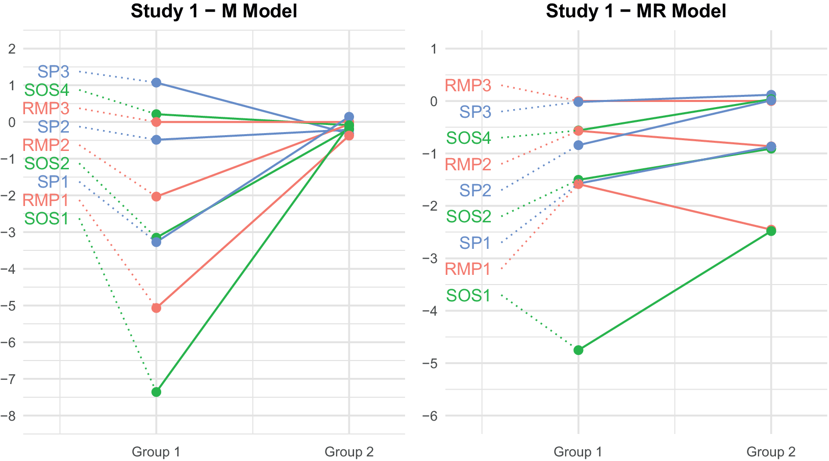
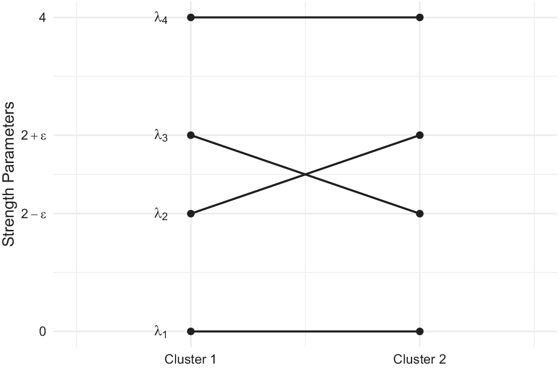


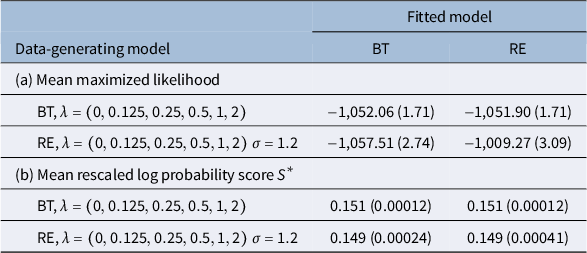

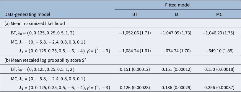

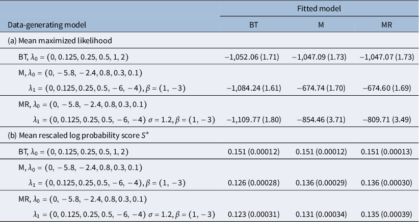

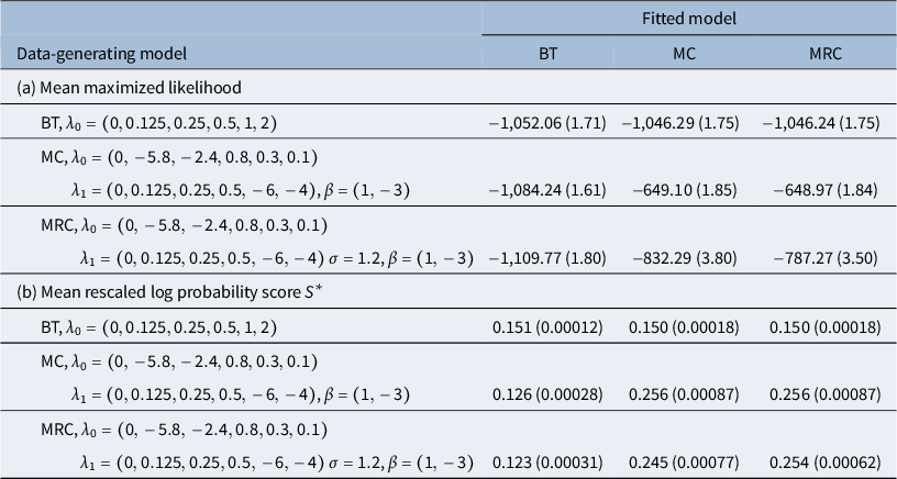



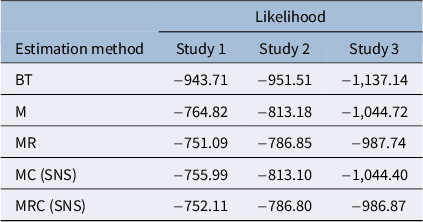

 Open access

