


Introduction
The degree to which ecological preferences are constrained by evolutionary history underpins the subdiscipline of phylogenetic community ecology. The prevailing paradigm is that evolutionary similarity can serve as a proxy for ecological similarity (Webb et al. Reference Webb, Ackerly, McPeek and Donoghue2002), but recent studies suggest this relationship is more complicated (Gerhold et al. Reference Gerhold, Cahill, Winter, Bartish and Prinzing2015; Cadotte et al. Reference Cadotte, Davies and Peres-Neto2017). The mechanism to explain the expected linear correlation between phylogenetic distance and ecological difference is evolution via competitive exclusion (MacArthur Reference MacArthur1958). Essentially, the idea is that speciation occurs as populations differentiate in order to coexist.
The assumption of a linear relationship based on competitive exclusion underlies studies of community phylogenetics and niche evolution; however, it is rarely tested. This assumption is problematic, for two main reasons. First, an apparent linear relationship between phylogeny and ecology can be produced by Brownian motion, especially over long timescales (Cadotte et al. Reference Cadotte, Davies and Peres-Neto2017). Second, there are ecological examples that counter competitive exclusion as the dominant assembly process (e.g., Hutchinson Reference Hutchinson1961), alternative hypotheses for community assembly (e.g., Hubbell Reference Hubbell2001), and suggestions that the processes of niche differentiation vary across spatial and temporal scales (e.g., Cardillo Reference Cardillo2011). Fossil phylogenies record evolution at large spatial and temporal scales, offering the opportunity to explore how ecological difference is related to evolutionary distance at scales at which evidence for competitive exclusion is not expected to be preserved. This is an important step toward placing constraints on possible models of niche evolution.
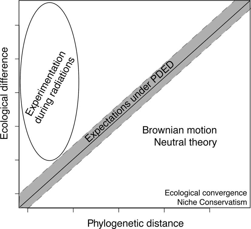
If phylogenetic distance and ecological difference do not covary linearly within a tree of fossil taxa, results can provide insight into other eco-evolutionary hypotheses (Fig. 1; see Hunt and Slater [Reference Hunt and Slater2016] for an overview of the applications of phylogenetics to macroevolution). If closely related taxa exhibit a wide range of ecologies, results would reflect a hypothesis of experimentation during times of radiation. Distantly related taxa with similar ecologies are examples of ecological convergence or niche conservatism. Finally, the region below the 1:1 linear correlation represents evolution via Brownian motion or neutral community assembly, suggesting that at larger scales, expected covariation might be obscured.
Expected phylogenetic distance, ecological difference relationship. Under the predictions of the phylogenetic distance/ecological difference (PDED), phylogenetic distance should be correlated with ecological difference. If species that are distantly related are ecologically similar, they would represent ecological convergence and/or niche conservatism. In contrast, if species that are closely related are ecologically different, they would represent high ecological plasticity such as what might be expected during an evolutionary radiation.

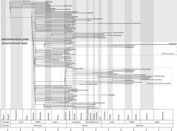
This paper explores the relationship between phylogenetic distance and ecological similarity across the Ordovician and Silurian for brachiopods from the order Strophomenida. This time period is important, because it contains the second largest Phanerozoic increase in diversity (the great Ordovician biodiversification event [GOBE]; Harper Reference Harper2006) and the second largest mass extinction (the Late Ordovician mass extinction [LOME]; Sheehan Reference Sheehan2001). We use recent evolutionary trees for this group (Congreve et al. Reference Congreve, Krug and Patzkowsky2015, Reference Congreve, Krug and Patzkowsky2019), synthesized into a composite tree (Fig. 2), to calculate phylogenetic distance. We combine this phylogenetic data with genus occurrence data from the Paleobiology Database to estimate environmental affinities. Comparing our results with modeled expectations (Fig. 1) provides insight into the evolution of ecology during intervals of increased origination and extinction rates.
Composite tree of Strophomenida scaled to stratigraphic range. This is a family-level phylogenetic analysis that contains 83 exemplar genera. Two main “groups” are identified within Strophomenida: a basal plectambonitoid grade (shaded region), which contains a clade of chonetids, and a clade of strophomenoids (unshaded region). Additionally, two important clades within the strophomenoid clade were identified (denoted by boxes with dashed lines): the rafinesquinids, which originated during the great Ordovician biodiversification event (GOBE) and survived the Late Ordovician mass extinction (LOME), and a recovery clade, which diversified during the aftermath of the LOME. Stratigraphic ranges (dark bars) are genus ranges from the Treatise on Invertebrate Paleontology (Cocks and Rong Reference Cocks, Rong and Kaesler2000).

Background
The Phylogenetic Distance/Ecological Difference Hypothesis
The phylogenetic distance/ecological difference (PDED; named in Cadotte et al. Reference Cadotte, Davies and Peres-Neto2017) hypothesis originates from Darwin (Reference Darwin1859) and was refined during the development of classical ecological theory (e.g., Mayr Reference Mayr1942; Brown and Wilson Reference Brown and Wilson1956; MacArthur Reference MacArthur1958). It states that the distance between species on a phylogenetic tree can serve as an estimate for the degree to which their ecological preferences differ. The utility of the PDED is in understanding species co-occurrence and community assembly, using the competitive exclusion principle (discussed in the following section).
However, there are many examples in modern ecology for which the competitive exclusion principle does not seem to apply. Perhaps the most well known is the “paradox of the plankton” (Hutchinson Reference Hutchinson1961), or the idea that phylogenetically distant plankton species coexist in pelagic environments despite limited resource availability, implying that competition does not control the distribution of plankton. Species in many other groups of organisms, such as plants (Shmida and Ellner Reference Shmida and Ellner1984), fish (Schlosser Reference Schlosser1982), deep-sea deposit feeders (Dayton and Hessler Reference Dayton and Hessler1972), and benthic mollusks (Stanley Reference Stanley2008), also appear to coexist with closely related species without much ecological differentiation and without one species driving others to extinction. Some explanations for a lack of competition are purely mathematical (Armstrong and McGehee Reference Armstrong and McGehee1980), but many invoke environments and species conditions that rapidly change over time and space (Hutchison Reference Hutchinson1961; Tilman et al. Reference Tilman, Kilham and Kilham1982; Chesson Reference Chesson1985; Huisman and Weissing Reference Huisman and Weissing1999), often employing stochastic biological models that simplify niche parameters (Chesson and Warner Reference Chesson and Warner1981; Cadotte et al. Reference Cadotte, Davies and Peres-Neto2017 and references therein). Ultimately, the role that competitive exclusion plays in community assembly is poorly understood.
The PDED hypothesis has been less explored in the fossil record. Several studies have used both phylogenetics and geometric morphometrics to draw upon the ideas behind the PDED to explain observed evolutionary patterns, using morphology as a proxy for ecology (e.g., Benton Reference Benton2009; Bapst et al. Reference Bapst, Bullock, Melchin, Sheets and Mitchell2011; Hopkins Reference Hopkins2014; Lamsdell et al. Reference Lamsdell, Congreve, Hopkins, Krug and Patzkowsky2017). However, none of these studies directly test whether morphology or phylogeny are actually correlated with ecology, as would be expected under the PDED. The pervasive nature of biofacies, or co-occurring groups of organisms with similar environmental affinities, throughout the geologic record (e.g., Ziegler Reference Ziegler1965; Ziegler et al. Reference Ziegler, Cocks and Bambach1968; Bretzky Reference Bretzky1969; Boucot Reference Boucot1983; Ludvigsen and Westrop Reference Ludvigsen and Westrop1983; Kammer et al. Reference Kammer, Brett, Boardman and Mapes1986; Brett and Baird Reference Brett, Baird, Erwin and Anstey1995; Patzkowsky and Holland Reference Patzkowsky and Holland2016) suggests that the data for unraveling the PDED for fossil species are available.
Community Assembly
The manner by which ecological communities assemble has been the subject of much debate. The two main hypotheses are niche-based and neutral-based assembly. Niche-based assembly is based on the classical competitive exclusion principle which states that species that rely on the same resource will not coexist in the same ecological community (Darwin Reference Darwin1859; Grinell Reference Grinell1922; Volterra Reference Volterra1926; Gause Reference Gause1934; Lack Reference Lack1947; MacArthur Reference MacArthur1958; Hardin Reference Hardin1960; see Whittaker et al. [Reference Whittaker, Levin and Root1973] for an overview of the evolution of the niche concept in classical ecology). The competitive exclusion principle is supported by some evidence (e.g., Lack Reference Lack1947; MacArthur Reference MacArthur1958; Chesson and Huntley Reference Chesson and Huntley1997; Violle et al. Reference Violle, Nemergut, Pu and Jiang2011), but there are many more examples of its effect on community structure being either more complicated than initially proposed (Dunson and Travis Reference Dunson and Travis1991; Goldberg and Barton Reference Goldberg and Barton1992; Tilman Reference Tilman1997; Huisman and Weissing Reference Huisman and Weissing1999; Mayfield and Levine Reference Mayfield and Levine2010; De Léon et al. Reference De Léon, Podos, Gardezi, Herrel and Hendry2014) or mostly negligible (Hutchinson Reference Hutchinson1961; Dayton and Hessler Reference Dayton and Hessler1972; Schlosser Reference Schlosser1982).
Despite these complications, niche-based assembly is often treated as the default assumption in ecological studies (e.g., Segre et al. Reference Segre, DeMalach, Henkin and Kadmon2016), with many efforts to increase the parameters of niche models (e.g., Soberon and Peterson Reference Soberon and Peterson2005; Godsoe Reference Godsoe2010; Wilson Reference Wilson2010), invoking the n-dimensional hypervolume (Hutchinson Reference Hutchinson1958) to explain the lack of competitive exclusion. Although these explanations appear to resolve the problems, they are often circumstantial and often lead to over-parameterized models, limiting their potential for broader theoretical application (Akaike Reference Akaike, Petrov and Csaki1973; see Johnson and Omland [Reference Johnson and Omland2004] and Warren and Seifert [Reference Warren and Seifert2011] for discussions of model selection criteria and model complexity in ecology).
Neutral theory is an alternative explanation for situations in which competitive exclusion does not apply (e.g., Hubbell Reference Hubbell2001, Reference Hubbell2005; Alonso et al. Reference Alonso, Etienne and McKane2006; Rosindell et al. Reference Rosindell, Hubbell and Etienne2010). Neutral theory is based on the island biogeography models of MacArthur and Wilson (Reference MacArthur and Wilson1967) and rests on the assumption that all species within a single trophic level of an ecological community are competitively equal. This assumption does not mean that all species have the same niches; rather, it is an extension of the concept of ecological functional groups (e.g., Grime Reference Grime1973; Walker Reference Walker1992; Wilson Reference Wilson1999; Bambach et al. Reference Bambach, Knoll and Sepkoski2002; Cadotte et al. Reference Cadotte, Carscadden and Mirotchnick2011) with the addition that any niche differences between members of a functional group are considered unimportant for assembling ecological communities.
Under neutral theory, the ability for any species to occupy space within a community is dependent on both its abundance within the community and dispersal ability. While many ecologists have criticized the simplicity of this model (e.g., Chesson and Huntley Reference Chesson and Huntley1997; Clark Reference Clark2009, Reference Clark2012; Purves and Turnbull Reference Purves and Turnbull2010), others have demonstrated its utility in explaining some of the complexity observed with purely niche-based models of community assembly (Tilman Reference Tilman2004; Leibold and McPeek Reference Leibold and McPeek2006), suggesting that communities are assembled via both competitive and stochastic processes (e.g., Adler et at. Reference Adler, HilleRisLambers and Levine2007; Cadotte Reference Cadotte2007).
Although they are often presented as opposing ideologies, it is perhaps more accurate to think of niche and neutral theory as end-member possibilities (McPeek Reference McPeek2007). It might be that both niche and neutral processes are important to structuring ecological communities, but their effects play out at different temporal or spatial scales (Leibold and McPeek Reference Leibold and McPeek2006; Chase and Myers Reference Chase and Myers2011). We liken this debate to whether biotic (Red Queen hypothesis; Van Valen Reference Van Valen1973) or abiotic (Court Jester; Barnosky Reference Barnosky2001) factors are more important for driving species evolution. A resolution to this dichotomy proposed a hierarchy of spatial and temporal scale where biotic factors are more important at small scales and abiotic factors are more important at regional scales and over a taxon's geologic range (Benton Reference Benton2009).
In community assembly, niche theory is a biotic perspective and neutral theory is a more abiotic perspective. If we place assembly processes in the same hierarchy, we can begin to resolve the current debate in a way that encourages more exchange of information between ecologists and paleoecologists working at different spatial and temporal scales. From this we can develop a broader, more comprehensive understanding of how ecological processes have changed throughout Earth's history.
Expectations for the Fossil Record
The question of how ecological processes change with spatial and temporal scale is especially important for understanding fossil ecological communities. Because of time averaging, or the accumulation of multiple ecological communities within a single lithologic bed, fossil assemblages generally represent the regional species pool (Kidwell Reference Kidwell2002). This means that the most appropriate theories for fossil community ecology are likely to be those that account for both time averaging and regional or metacommunity dynamics (see Patzkowsky [2017] for a discussion of the role of regional dynamics in paleoecology).
Additionally, several studies have used neutral dynamics to successfully explain observed spatial and temporal turnover of fossil ecological communities (Olszewski and Erwin Reference Olszewski and Erwin2004; Tomasovych and Kidwell Reference Tomasovych and Kidwell2010; Sclafani and Holland Reference Sclafani and Holland2013; Wang et al. Reference Wang, Chen, Fang and Pacala2013; Holland and Sclafani Reference Holland and Sclafani2015; Holland Reference Holland2018). A possible explanation for neutrality in fossil ecological communities is that at the long timescales preserved in the fossil record, competitive exclusion and other niche processes might be obscured by more neutral dynamics. Because the PDED hypothesis rests on an assumption of niche-based assembly rules, its effects might similarly be difficult to distinguish within (potentially) stochastically assembled fossil communities.
Biofacies, or assemblages of co-occurring fossil taxa with similar environmental affinities, are prevalent throughout the fossil record (e.g., Ziegler Reference Ziegler1965; Ziegler et al. Reference Ziegler, Cocks and Bambach1968; Bretzky Reference Bretzky1969; Boucot Reference Boucot1983; Ludvigsen and Westrop Reference Ludvigsen and Westrop1983; Kammer et al. Reference Kammer, Brett, Boardman and Mapes1986; Brett and Baird Reference Brett, Baird, Erwin and Anstey1995; Patzkowsky and Holland Reference Patzkowsky and Holland2016; for more complete reviews of ecological stability in the fossil record, see Morris [Reference Morris1996] and Schopf [Reference Schopf1996]). Biofacies are consistent assemblages, tied to certain depositional environments, and persist over long intervals of geologic time. In an ecological context, biofacies can be considered to represent the regional species pool, such that general stability through time suggests that the niches of constituent species are conserved. However, their long-term stability does not mean that biofacies were assembled by competitive exclusion. Random processes also can create a stable system, as in the mathematical stable-roommate problem in which a system can be stably assembled in any configuration of pairs as long as no member prefers a different partner (Irving Reference Irving1985). Ecologically, this suggests that if environmental affinity is weak, randomly assembled stable configurations exist because chances are low that a species would prefer something other than their random assignment.
Whether niches evolve on geologic timescales is a pressing question in paleobiology (e.g., Holland and Zaffos Reference Holland and Zaffos2011; Saupe et al. Reference Saupe, Hendricks, Portell, Dowsett, Haywood, Hunter and Lieberman2014; Qiao et al. Reference Qiao, Saupe, Soberón, Peterson and Myers2016). The idea that niches might shift or be conserved over geologic time and that this pattern should be detectable in the fossil record forms the basis of our exploration of how the ecology of strophomenide brachiopods evolved. Because of the resolution available in the fossil record, a substantial amount of data used in paleoecological studies is at the genus or family level, including many biofacies. This is operationally acceptable (Patzkowsky Reference Patzkowsky2017) and supported by studies that have demonstrated that genera have niches that are composed of the niches of their constituent species (e.g., Smith et al. Reference Smith, Brown, Haskell, Lyons, Alroy, Charnov, Dayan, Enquist, Ernest, Hadly, Jablonski, Jones, Kaufman, Marquet, Maurer, Niklas, Porter, Roy, Tiffney and Willig2004; Hadly et al. Reference Hadly, Spaeth and Li2009; Foote et al. Reference Foote, Ritterbush and Miller2016; Patzkowsky and Holland Reference Patzkowsky and Holland2016). Within this framework, ecological data can be derived from lithological parameters that serve as proxies for an organism's realized niche. Niche interpretations from environmental data preserved in the rock record contain limited parameters compared with modern environments but produce analogous results that have been successfully employed in numerous paleobiological studies (Holland and Zaffos Reference Holland and Zaffos2011; Saupe et al. Reference Saupe, Hendricks, Portell, Dowsett, Haywood, Hunter and Lieberman2014; Myers et al. Reference Myers, Stigall and Lieberman2015; Nawrot et al. Reference Nawrot, Scarponi, Azzarone, Dexter, Kusnerik, Wittmer, Amorosi and Kowalewski2018).
Note that although ecological data used in this study are at the genus level, phylogenetic data used in this study are at the species level, such that each tip of the phylogeny represents a single species within a genus. Despite this limitation of resolution, the fossil record is ripe with ecological data that inform and are informed by long-term evolutionary patterns. Although assemblages of fossil organisms are rarely equivalent to modern ecological communities, they do contain vital information about the regional species pool and offer insight into how biodiversity changes on timescales that would be otherwise unknowable.
Expectations for Strophomenida
We examined phylogenetic (Congreve et al. Reference Congreve, Krug and Patzkowsky2015, Reference Congreve, Krug and Patzkowsky2019) and ecological (Paleobiology Database) data from the same brachiopod genera within the order Strophomenida to identify correlations and gain insight into the evolutionary process. A correlation between phylogenetic distance and ecological difference would suggest that the competitive exclusion principle scales in an identifiable way and is responsible for diversification of strophomenides. If phylogenetic distance and ecological difference are not correlated, more neutral or stochastic processes were likely responsible for generating strophomenide diversity.
Methods
Phylogenetic Data
Phylogenetic data were gathered from recent revisions to the brachiopod order Strophomenida, which ranges from the Early Ordovician to the Carboniferous (Congreve et al. Reference Congreve, Krug and Patzkowsky2015, Reference Congreve, Krug and Patzkowsky2019). A composite tree of these two studies scaled to stratigraphic range (Fig. 2) contains 83 exemplar genera from all but one family (Foliomenidae, which was removed, because the analyses could not resolve its phylogenetic position within the order). This family-level phylogenetic analysis identified two “groups” within Strophomenida: a basal plectambonitoid grade, which contains a clade of chonetids, and a clade of strophomenoids. Additionally, two important clades within the strophomenoid clade were identified: the rafinesquinids, which originated during the GOBE and survived the LOME, and a recovery clade, which diversified during the aftermath of the LOME. Highlighting the PDED in these smaller groups will allow an assessment of whether the variability (eurytope vs. stenotope) in environmental affinity conferred any survival advantages during the LOME.
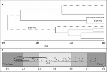
Pairwise phylogenetic distances between each taxon in the phylogeny were calculated using the cophenetic.phylo function in the ape package (Paradis and Schliep Reference Paradis and Schliep2018) of R (R Core Team 2018). This function calculates the distance between tips of the tree by measuring the branch length between them (see Fig. 3A for a visual depiction of how this works). Branch lengths were calculated using basic, minimum branch length (mbl), and equal branch length with the R package paleotree (Bapst Reference Bapst2012). The basic time calibration pulls the origin of groups back to the earliest possible time, whereas the mbl uses the latest possible time. The equal branch length method provides an estimate in the middle. To minimize biases introduced by favoring long or short branch lengths, results from the equal calibration are reported here; however, results were similar for all calibration methods (see Supplementary Material for results from basic and mbl). Because the composite tree (Fig. 2) is scaled to stratigraphic range, branch lengths here were calculated in units of millions of years, which represent the time since divergence for each taxon pair. Each distance was classified in terms of whether the measurements were within-group (pairs that are in the same evolutionary group) or between-group (pairs that are in different evolutionary groups).
Pairwise distance calculations. This is a hypothetical example of the methods used to calculate pairwise distances. A, Phylogenetic distance was calculated as branch length between each pair of tips on the tree. B, Ecological difference was calculated as distance between each pair of points along the binary environmental gradient (see “Methods”). Each “x” represents a taxon of interest.

Ecological Data
Environmental affinities are used here as a metric for ecology. This assessment of ecology is based on lithologic and locality data that co-occur with fossils. Brachiopod occurrence data were downloaded from the Paleobiology Database in February 2019. Environmental data available for fossil taxa in this download include the depositional environment relative to shoreline (a proxy for all of the variables that covary with water depth), substrate type (carbonate or siliciclastic), and paleolatitude (as determined by the Paleobiology Database Application Programming Interface using gplates).
Previous studies indicate that relative water depth (as determined by depositional environment) and substrate are the most important variables for explaining regional genus distributions (Holland and Patzkowsky Reference Holland and Patzkowsky2004, Reference Holland and Patzkowsky2007, Reference Holland and Patzkowsky2009; Nawrot et al. Reference Nawrot, Scarponi, Azzarone, Dexter, Kusnerik, Wittmer, Amorosi and Kowalewski2018), whereas environmental factors that vary with latitude, such as temperature, productivity, and ocean currents, control distribution at the global scale (Roy et al. Reference Roy, Jablonski and Martien2000; Jablonski et al. Reference Jablonski, Roy and Valentine2006, Reference Jablonski, Belanger, Berke, Huang, Krug, Roy, Tomasovych and Valentine2013; Valentine et al. Reference Valentine, Jablonski, Krug and Roy2008; Powell Reference Powell2009). These proxies can be evaluated in the geologic record and reflect a myriad of co-occurring physical and chemical factors that drive taxonomic distribution in the modern oceans. Combined, they are an approximation of the realized niche, proxies for the abiotic factors that these organisms require for survival.
Affinity calculations are based on a previous method developed by Simpson and Harnik (Reference Simpson and Harnik2009) and applied by Hopkins (Reference Hopkins2014). This study modifies the calculation from Simpson and Harnik (Reference Simpson and Harnik2009) to indicate the strength of environmental preference along a continuous environmental gradient. Early tests of the Simpson and Harnik (Reference Simpson and Harnik2009) method on brachiopod occurrence data discretized the environmental binary in a manner that did not reflect our understanding of marine environmental gradients in the fossil record (Holland and Patzkowsky Reference Holland and Patzkowsky2004, Reference Holland and Patzkowsky2007, Reference Holland and Patzkowsky2009). The modified equation presented in this study is an adjustment of the ideas behind previous affinity calculations that standardized Paleobiology Database occurrences against data available (e.g., Foote Reference Foote2006; Kiessling and Aberhan Reference Kiessling and Aberhan2007; Simpson and Harnik Reference Simpson and Harnik2009; Anderson et al. Reference Anderson, Pisani, Miller and Peterson2011; Thompson and Bottjer Reference Thompson and Bottjer2019). The method presented here differs from the others in that it calculates the strength of preference in a manner that allows study taxa to be arranged along an environmental gradient between two binary environmental states. See Hopkins (Reference Hopkins2014) and Thompson and Bottjer (Reference Thompson and Bottjer2019) for full comparative discussions of many of the other methods for calculating environmental affinity.
Environmental data (water depth, substrate, paleolatitude) associated with taxonomic occurrences from the Paleobiology Database download were used to calculate environmental affinities using the following equation:
 $$A_x = \displaystyle{{\mathop \sum \nolimits^ T_x} \over {\mathop \sum \nolimits^ T_x + \mathop \sum \nolimits^ T_y}}-\displaystyle{{\mathop \sum \nolimits^ O_x} \over {\mathop \sum \nolimits^ O_x + \mathop \sum \nolimits^ O_y}}\comma \;$$
where x and y represent each side of an environmental binary (e.g., deep/shallow-water environments, carbonate/siliciclastic substrate, tropical/extratropical latitudes). For example, if x is deep water, then this equation would calculate whether the proportion of deep-water occurrences of the taxon of interest (T) is greater than, equal to, or less than the proportion of deep-water occurrences of all taxa being evaluated (O).
Proportional occurrences of each strophomenide genus (T) are compared with the proportional occurrences of all Ordovician through Devonian brachiopod genera in the Paleobiology Database (O). Using the proportion of occurrences is necessary to control for variation in sampling between genera and environments. Comparing strophomenide genus occurrences with all brachiopod occurrences corrects for differences in sampling intensity between groups. Essentially, if a rock yielded brachiopods, it could have yielded strophomenide brachiopods, but whether it did depends on whether the rock was deposited under environmental conditions favorable to strophomenides.
The resulting value is the strength of the taxon of interest's preference for those environments, or its affinity, relative to all taxonomic occurrences considered in the dataset. If Ax is greater than zero, the taxon has more deep-water occurrences than expected within the dataset, or an affinity for deep water. If Ax is less than zero, the taxon has fewer deep-water occurrences than expected within the dataset, or an affinity for shallow water. If Ax equals zero, the taxon has the same number of deep-water occurrences as expected within the dataset, or no affinity for deep or shallow water. This affinity calculation generates an environmental affinity gradient for the phylogeny and provides a relative assessment of how each genus was distributed across benthic environments. Taxa at either end of the gradient have a strong preference, while taxa in the middle have a weak or no preference.
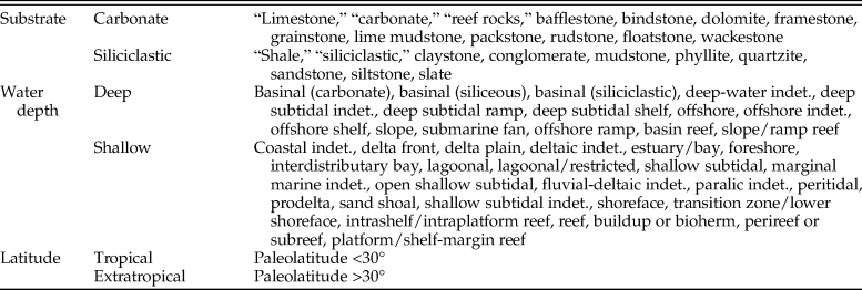
Environmental data from the Paleobiology Database were vetted before being included. Any genus without environmental data was necessarily excluded. Additionally, any genus with fewer than 15 occurrences was removed in order to minimize the weight of a single occurrence in the environmental binaries. Environmental data were culled according to the methods in Foote (Reference Foote2014), which used only the primary lithology field and removed anything that could not be assigned to either a carbonate or clastic category. Criteria for classification into relative water depth, lithologic, and paleolatitude binaries are outlined in Table 1 (based on Hopkins Reference Hopkins2014). Pairwise distances were calculated between the locations of each taxon along this modeled environmental affinity gradient (Fig. 3B).
Scheme for categorizing environmental variables. This scheme was applied to brachiopod data downloaded from the Paleobiology Database. Substrate names are from the “lithology1” field. Water-depth names are from the “environment” field. Latitude is from the “paleolat” field. Classification into these binary groups is based on the classification scheme used in Hopkins (Reference Hopkins2014).

Results
Environmental Affinities
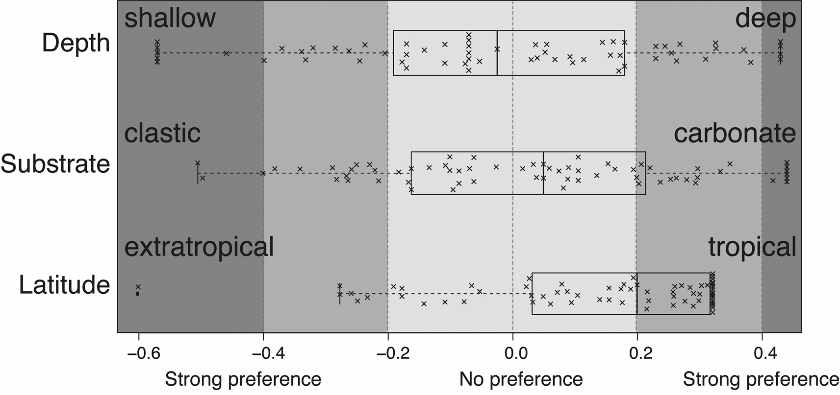
Environmental affinity calculations demonstrate that on average, Strophomenida as a group has no affinity for deep water and only weak affinity for carbonate substrates compared with all brachiopods. However, variability between genera is high (Fig. 4). Genus water-depth affinities have a median of −0.02 and range from −0.19 to 0.18 between the 1st and 3rd quartile. For substrate, genus affinities have a median of 0.05 and range from −0.17 to 0.21 between the 1st and 3rd quartile. Because of the large range in affinities, arranging values for each genus in a box-and-whisker plot as a simulated environmental gradient (Fig. 4) highlights that despite no overall ordinal preference for depth or lithology, almost half of all constituent genera display a moderate to strong preference for either extreme of the depth and lithology binary.
Environmental affinities of Strophomenida compared with distribution of all brachiopod occurrences. Results of the calculation of environmental affinity for each genus in the composite tree (Fig. 2). The line inside the box is the median, the edges are the first quartile, and the whiskers mark the extremes. Each “x” represents a Strophomenida genus. Vertical offset of points within each box plot is just to improve visualization of the data and has no scientific meaning.

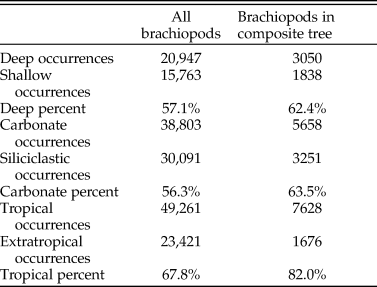
Strophomenida does occur more often in rocks classified as deep or carbonate (greater than 62%), compared to just over 56% of all Ordovician to Devonian brachiopod occurrences in the Paleobiology Database (Table 2). However, the occurrence percentages of the order are influenced by a few highly abundant genera such as Strophomena and Rafinesquina (1395 and 1519 occurrences, respectively). These two genera combined make up more than 30% of all Strophomenida occurrences and almost 60% of Strophomenida occurrences with depth data. Both genera have weak preferences for deep-water environments (0.07 for Strophomena and 0.09 for Rafinesquina) and weak to moderate preferences for carbonate environments (0.16 for Strophomena and 0.25 for Rafinesquina). The distribution of genus environmental affinities across the simulated environmental gradient can account for the weight that abundant genera give to occurrence percentages. Despite the slight preference for deep, carbonate environments of the two most abundant genera, as a whole, Strophomenida genera included in this study, do not prefer deep, carbonate environments more than the average for brachiopod occurrences in the Paleobiology Database.
Strophomenida environmental preferences. Occurrence values are reported for all brachiopod genera from the Ordovician to Devonian in the Paleobiology Database and for brachiopod genera in the composite tree used in this study. The majority of genus occurrences were in rocks that were classified as deep, carbonate, and tropical, indicating a preference for these environments.

In contrast, Strophomenida has a strong preference for tropical latitudes (between 30°N and 30°S). This is consistent with the percent occurrence of strophomenide genera in tropical latitudes (just over 80%) compared with 68% of all brachiopod occurrences (Table 2). While latitudinal occurrences might also be influenced by abundant genera, the spread of genus affinities is not as great. Along the environmental gradient (Fig. 4), about 75% of all genera fall on the tropical side of the binary and more than 50% have a strong preference for tropical environments. This means that for most genera, latitude preferences are consistent with that for the order as a whole. It also suggests that Strophomenida might be slightly more tropical than most brachiopods.
In summary, the disparity in environmental preference varies for genera within Strophomenida. Both relative water depth and substrate preferences are very disparate, resulting in an ordinal preference that averages out the extremes, whereas latitudinal preference is relatively conserved throughout Strophomenida genera. This suggests a strong biogeographic control on Strophomenida global distribution (consistent with Congreve et al. Reference Congreve, Krug and Patzkowsky2019), but weak niche differentiation at regional spatial scales.
Phylogenetic Distance/Ecological Difference
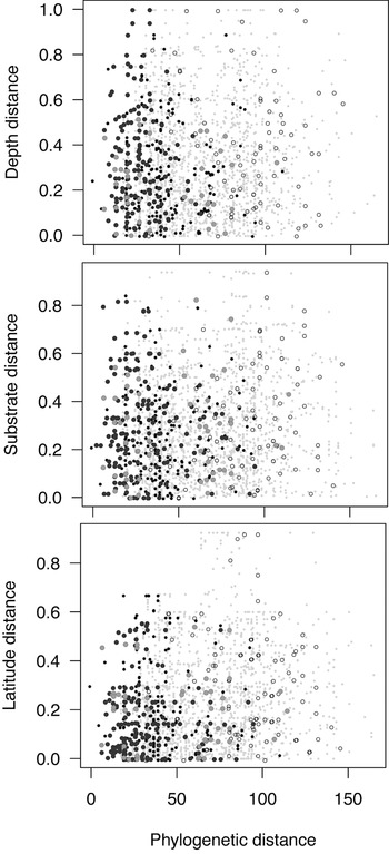
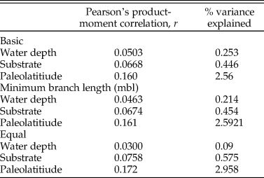
Phylogenetic distance is not correlated with environmental affinity distance (Fig. 5, Table 3). The correlation is equally poor for all three of the environmental variables and all three time-calibration methods. Although visualizations of these data (Fig. 5) appear to be correlated, no correlation explains more than 3% of the variation in the data. Given the large sample size (more than 1000 pairwise comparisons) and the known impact of effect size (Holland Reference Holland2019), it is necessary to ignore the apparent significance of the correlation and instead focus on the percent variance explained (the square of the correlation coefficient). Because the correlation coefficient is extremely low, other unexplored parameters are more important for the variation in ecological difference examined in this study. This means that for the environmental parameters explored here, there is no correlation between phylogenetic distance and ecological difference for strophomenide brachiopods.
Pairwise distances for Strophomenida composite tree. The equal time calibration method is shown here. Points are color coded based on evolutionary group membership of taxa in the pairwise comparison. Small black points indicate both taxa are in the basal grade. Dark gray indicates both taxa are in the strophomenoid clade. Light gray indicates both taxa are in the rafinesquinid clade. Open circles indicate both taxa are in the recovery strophomenoid clade. Light gray smaller points indicate taxa are in different groups.

Pearson correlation statistics. Values are for a correlation between phylogenetic distance and each variable listed. Calculations were made for all time calibration methods. The percent variance explained is less than 3% for all environmental variables.

Discussion
Results indicate that this group of strophomenide brachiopods shows no clear relationship between phylogenetic distance and ecological difference. In the following sections, we address methodological caveats that are important to recognize but do not invalidate the results.
One potential explanation for the lack of relationship between strophomenide phylogeny and ecology is the quality and quantity of environmental data in the Paleobiology Database. Of those data used here, the depositional environment data that form the water depth proxy are the most potentially problematic, because this interpretation was historically absent from fossil occurrences. In contrast, substrate and latitude are fairly robust, because a carbonate or siliciclastic substrate designation is inherent in rock type identification and the Paleobiology Database automatically calculates latitude based on collection locality and paleogeographic reconstructions. This means that every occurrence had usable latitude data, while only about 50% had usable depth data. The total number of occurrences for each environmental variable for strophomenide brachiopods can be found in Table 2.
If the lack of relationship between phylogeny and ecology was due simply to data quality, we might expect an improvement with the variables that are likely to be more accurate. As there is no improvement in the relationship for latitude and substrate, we conclude that the environmental variables available are not important for explaining evolutionary history within Strophomenida. However, the large spread in genus affinities for relative water depth and substrate suggest some environmentally related niche differentiation occurred along the marine shelf. This apparent disconnect between what drives spatial distribution of genera and what drives diversification for this order is an avenue for future research.
Another potential explanation for the lack of PDED correlation within these brachiopods is the coarse phylogenetic resolution of the study. That is, species included in the composite phylogeny are exemplars for genera. Because the PDED rests on an assumption of competitive exclusion, to truly see its effect, a phylogeny would need to include true sister species, that is, the two species that are the product of a single speciation event. However, it is extremely difficult to identify exact speciation events at macroevolutionary timescales (Mayr Reference Mayr1982; Rabosky Reference Rabosky2013). Additionally, in the fossil record, some sister species might not have been successful enough or abundant enough to be preserved. If taxonomic scale were the only factor influencing these results, that is, if remnants of divergence due to competitive exclusion could be identified from more distant relatives, we might expect a better correlation for within-clade pairs than for between-clade pairs. Instead, pairwise comparisons focusing only within clades do not improve the relationship (Fig. 5).
Despite these caveats, we argue that the lack of PDED correlation for Strophomenida highlights the need for further research into the conditions under which evolutionary history and ecological preference are correlated throughout geologic time. Additional studies quantifying the parameters of this model for other fossil groups are needed. In the following sections, we outline two possible explanations that we feel are particularly important for Strophomenida and that we hope will fuel larger research efforts to understand the relationship between evolution and ecology in the fossil record.
The Evolution of Ecologies during Radiations
The order Strophomenida was affected by two radiations: the GOBE during the Middle Ordovician (Harper Reference Harper2006; Congreve et al. Reference Congreve, Krug and Patzkowsky2019) and the Silurian recovery from the LOME (Sheehan Reference Sheehan2001; Congreve et al. Reference Congreve, Krug and Patzkowsky2015; Sclafani et al. Reference Sclafani, Congreve, Krug and Patzkowsky2018). Lineage diversification is mostly restricted to these two time intervals. It is possible that morphological and ecological experimentation during times of rapid evolution results in more disparity than would be expected for closely related species under the PDED expectation. This is because once a new clade originates, rates of diversification are rapid as new species evolve to fill available adaptive space (Van Valen Reference Van Valen1985; Sepkoski Reference Sepkoski1991; Patzkowsky Reference Patzkowsky1995; Jablonski Reference Jablonski2005). If a clade experiencing a radiation is more morphologically plastic, as some suggest, (Erwin Reference Erwin2007, Reference Erwin2015; Wood and Erwin Reference Wood and Erwin2017), members of the clade might explore a wider range of ecologies than predicted simply by phylogenetic distance.
There is significant debate in the fields of paleobiology and modern biology about the degree to which an organism's ecology is controlled by either contingent properties of an organism's evolutionary history (i.e., phylogenetic constraint) or as the result of adaptation to changing environments (i.e., morphological novelty) (Wood and Erwin Reference Wood and Erwin2017). Many of these questions are fundamental to understanding the adaptive potential of organisms during times of environmental crisis. The results of this study provide a more concrete picture of the complexity involved in untangling the effects of evolution and ecology on a radiating clade. More work is needed on potentially convergent and constrained strophomenide morphologies; specifically focusing on widespread convergence across this clade's geologic range and improving the understanding of ecologically meaningful morphologies will allow us to better understand potential links between ecology and phylogeny. From this foundation, rates of ecological character change during radiations can be compared with rates of change during background intervals.
Metacommunity Theory and Hierarchical Scaling in Paleoecology
Beginning with Darwin (Reference Darwin1859), evolutionary biologists and paleobiologists have cited incomplete sampling as an explanation for a lack of support for many evolutionary and ecological hypotheses in the fossil record. This has historically created a barrier to communication between these disciplines. There are certainly time intervals and geographic regions that are undersampled. While targeted sampling efforts can help fill some of the gaps, they are unlikely to provide support for microecological theories. Because of time averaging, the fossil record preserves biological data at a fundamentally larger temporal and spatial scale than that which is observable in modern ecological communities (e.g., Kidwell Reference Kidwell2002). Fossil assemblages represent the regional species pool quite well, but rarely preserve individuals that interacted in ecological time. In many cases, it is not that the data have not been sampled, it is that the data do not exist at the spatial and temporal resolution available in modern observational ecology. This does not mean fossil data are not useful, but that they are best suited for different types and scales of analyses.
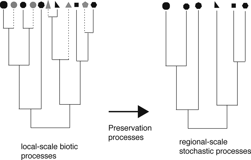
The inherent difference in scale between modern data and the fossil record means that fossil evolutionary trees are pruned by preservation such that ecological communities do not include many short-lived and rare taxa (Fig. 6). If they were preserved and sampled, these taxa could lend support for microevolutionary hypotheses of community assembly, such as the PDED, that are rooted in small spatial and short temporal scales. However, for much of the fossil record, processes emergent at the macroevolutionary and macroecological scales (e.g., species sorting, neutral community assembly) dominate the signal. This disconnect in scale is likely due to the nested hierarchical nature of ecological entities, where each level of the hierarchy (organisms, populations, communities, metacommunities, ecosystems) is composed of groups from the lower level (Vrba and Eldredge Reference Vrba and Eldredge1984). Complex interactions within this hierarchy form emergent properties at each hierarchical level, which in turn can act to diminish the impact that changes occurring in lower levels of the hierarchy have on higher hierarchical levels (Congreve et al. Reference Congreve, Falk and Lamsdell2018). Given the macroecological scale of these data and the nature of these nested hierarchical systems, it is perhaps expected that results did not support the PDED model. Similarly, modern studies conducted at macroecological scales also tend to not support the PDED (Cadotte et al. Reference Cadotte, Davies and Peres-Neto2017). Consistent with the compromise for the Red Queen and Court Jester hypotheses (Benton Reference Benton2009), scale affects whether biotic or abiotic factors primarily drive evolution. It is thus necessary to consider how processes scale through the dual hierarchy theory of evolution and ecology (Vrba and Eldredge Reference Vrba and Eldredge1984; Congreve et al. Reference Congreve, Falk and Lamsdell2018 and references therein).
The effect of preservation and sampling on fossil phylogenies. Preservation processes result in a phylogeny that does not preserve all of the evolutionary experimentation that might have occurred in local communities over short timescales. Instead, the phylogeny contains only those species that persisted long enough and at large enough abundance to be preserved. This fossil phylogeny reflects the larger species pool and allows for macroevolutionary and metacommunity analyses. However, species differ more than expected under competitive exclusion, which makes the fossil phylogeny unlikely to support the phylogenetic distance/ecological difference model.

This hierarchy of scale highlights a fundamental difference between paleoecology and modern ecology and illustrates a need for these disciplines to inform each other. Understanding the processes driving biodiversity under these two very different regimes requires an understanding of the differences in the type of data available to each discipline and an acceptance of the importance of spatial and temporal scaling. Ultimately, assessments of ecological communities in the fossil record should center on macroecology and neutral theory, both of which are connected to metacommunity theory. And yet, none of this discounts the observations at small scales that support niche-based assembly in modern datasets.
Instead, our results support arguments for the combined effect of both neutral and niche processes of community assembly and the importance of spatial and temporal scale in averaging out ecological processes. Perhaps neutral dynamics dominate at the metacommunity scale, and niche dynamics can only be observed at much smaller spatial and temporal scales. This would explain why there is no detectable PDED relationship for strophomenide brachiopods; any such relationship would be averaged out at the metacommunity scale. Moving forward, it is important to focus research efforts on understanding how ecological and evolutionary processes scale up so that we can better explain biodiversity patterns in the fossil record and make predictions for the present biodiversity crisis.
Conclusions
The results of this analysis demonstrate no correlation between phylogenetic distance and ecological difference for strophomenide brachiopods. This result is indicative of a fundamental difference in the ecological and evolutionary processes observable with fossil data as compared to that observable in the modern, reflecting a hierarchy of scale. The fossil record preserves organisms at the metacommunity scale. At this scale, neutral processes dominate over competitive exclusion. This interpretation is not intended to support either side of the neutral–niche debate. Instead, both processes are important, albeit at different spatial and temporal scales. Untangling the relationship between difference scales is an avenue for future research.
Acknowledgments
We thank G. Brown, M. Christie, S. M. Holland, A. Z. Krug, and J. C. Lamsdell for various comments, thoughts, and discussions during early stages of this project. We thank T. Bralower, D. Hughes, and P. Wilf for comments provided via service on J. A. Sclafani's dissertation committee. We thank the creators of the Paleobiology Database for making this resource available and the following people for contributing to the majority of the data used in this study: P. Wagner, M. Foote, P. Novack-Gottshall, B. Kröger, J. Ju, U. Merkel, T. Hanson, K. Layou, and P. Hearn (see Supplementary Material for full list of data authors and enterers). Thanks to B. Anderson and J. Bauer for their reviews, which improved the quality of this article. This research was partially funded by NASA Astrobiology grant 11-EXO11-0070. This is Paleobiology Database official publication number 375.