2. Evolution equations

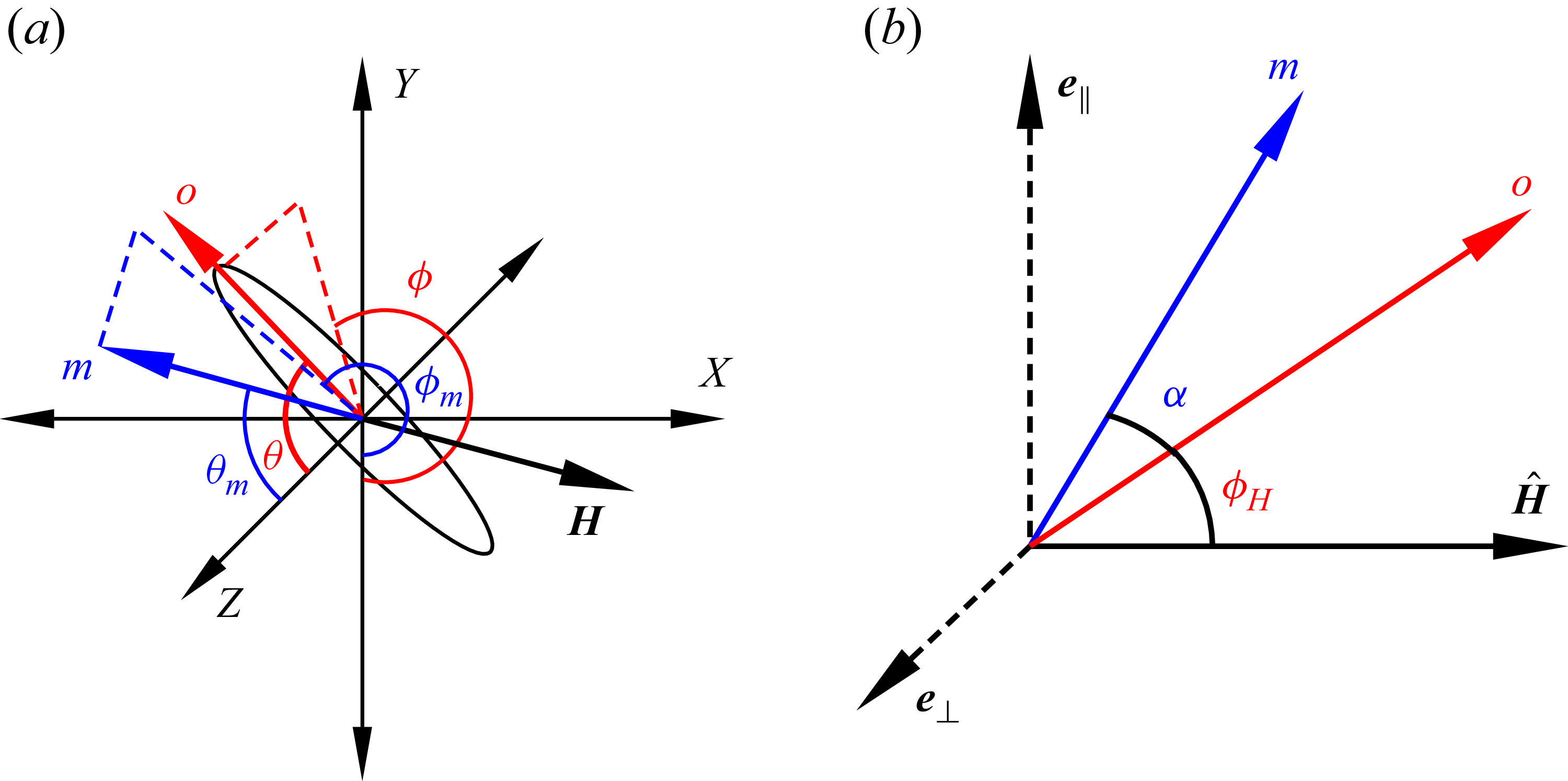
A magnetic field $\boldsymbol{H}$ rotating with an angular velocity $\boldsymbol{\omega } = \omega \boldsymbol{\hat {Z}}$ and magnitude $H$ acts on a magnetic spheroid with orientation unit vector $\boldsymbol{o}$ , as shown in figure 1(a). The plane of rotation of the magnetic field is the $X$ – $Y$ plane. The azimuthal angle $\theta$ is the angle between the orientation vector $\boldsymbol{o}$ and the $Z$ axis, and the meridional angle $\phi$ is the angle between the projection of the orientation vector in the $X$ – $Y$ plane and the – $Y$ axis in the fixed reference frame. The components of $\boldsymbol{o}$ and $\boldsymbol{H}$ are

(2.1) \begin{align} \boldsymbol{o} & = \sin {(\theta )} \sin {(\phi )} \boldsymbol{e}_X - \sin {(\theta )} \cos {(\phi )} \boldsymbol{e}_Y + \cos {(\theta )} \boldsymbol{e}_Z, \\[-12pt] \nonumber \end{align}

(2.2) \begin{align} \boldsymbol{H} & = H(\sin {(\omega t)} \boldsymbol{e}_X - \cos {(\omega t)} \boldsymbol{e}_Y). \\[9pt] \nonumber \end{align}

The dot product of $\boldsymbol{o}$ and $\boldsymbol{H}$ is

(2.3) \begin{eqnarray} \boldsymbol{o} \boldsymbol{\cdot } \boldsymbol{H} & = & H \sin {(\theta )} \cos {(\phi ')}, \end{eqnarray}

where $\phi ' = \phi - \omega t$ is the meridional angle in the reference frame rotating with the magnetic field. The magnetic moment of magnitude $|\boldsymbol{m}| = m$ makes an angle $\alpha$ with $\boldsymbol{o}$ in the plane containing $\boldsymbol{H}$ and $\boldsymbol{o}$ , as shown in figure 1(b).

Figure 1.

Configuration and coordinate system of a spheroid subjected to a rotating field $\boldsymbol{H}$ with axis of rotation in the $Z$ direction. Panel (a) shows the orientation vector of the spheroid $\boldsymbol{o}$ (red) defined by azimuthal angle $\theta$ with respect to $Z$ axis and meridional angle $\phi$ with respect to $-Y$ axis, and magnetic moment $\boldsymbol{m}$ (blue) defined by azimuthal angle $\theta _m$ with respect to $Z$ axis and meridional angle $\phi _m$ with respect to $-Y$ axis. Panel (b) shows the relative orientation of the magnetic field direction $\kern1pt \hat {\boldsymbol{\kern-1pt H}}$ , the orientation vector $\boldsymbol{o}$ and the magnetic moment $\boldsymbol{m}$ in the same plane. The unit vector $\boldsymbol{e}_\parallel$ is perpendicular to $\boldsymbol{\hat{H}}$ in the $\kern1pt \hat {\boldsymbol{\kern-1pt H}}\!-\!\boldsymbol{o}$ plane, and $\boldsymbol{e}_{\perp }$ perpendicular to the $\kern1pt \hat {\boldsymbol{\kern-1pt H}}{-}\boldsymbol{o}$ plane. The angle from the magnetic field to the orientation vector is $\phi _H$ and that from the orientation vector to the magnetic moment is $\alpha$ .

An orthogonal coordinate system shown in figure 1(b) is defined in the rotating reference frame, in which the unit vector $\kern1pt \hat {\boldsymbol{\kern-1pt H}}$ is along the magnetic field direction, the unit vector $\boldsymbol{e}_\parallel$ is perpendicular to $\kern1pt \hat {\boldsymbol{\kern-1pt H}}$ in the $\kern1pt \hat {\boldsymbol{\kern-1pt H}}{-}\boldsymbol{o}$ plane, and $\boldsymbol{e}_{\perp }$ is perpendicular to the $\kern1pt \hat {\boldsymbol{\kern-1pt H}}{-}\boldsymbol{o}$ plane,

(2.4) \begin{align} \kern1pt \hat {\boldsymbol{\kern-1pt H}} & = \sin {(\omega t)} \boldsymbol{e}_X - \cos {(\omega t)} \boldsymbol{e}_Y, \\[-12pt] \nonumber \end{align}

(2.5) \begin{align} \boldsymbol{e}_{\parallel } & = \frac {(\boldsymbol{I} - \kern1pt \hat {\boldsymbol{\kern-1pt H}} \kern1pt\! \hat {\boldsymbol{\kern-1pt H}}) \boldsymbol{\cdot } \boldsymbol{o}}{|(\boldsymbol{I} - \kern1pt \hat {\boldsymbol{\kern-1pt H}} \kern1pt\! \hat {\boldsymbol{\kern-1pt H}}) \boldsymbol{\cdot } \boldsymbol{o}|} \nonumber \\& = \frac {\sin {(\theta )} \sin {(\phi ')} \cos {(\omega t)} \boldsymbol{e}_X + \sin {(\theta )} \sin {(\phi ')} \sin {(\omega t)} \boldsymbol{e}_Y + \cos {(\theta )} \boldsymbol{e}_Z}{\sqrt { \sin {(\theta )}^2 \sin {(\phi ')}^2 + \cos {(\theta )}^2}}, \\[-12pt] \nonumber \end{align}

(2.6) \begin{align} \boldsymbol{e}_{\perp } & = \frac {\kern1pt \hat {\boldsymbol{\kern-1pt H}} \times \boldsymbol{o}}{|\kern1pt \hat {\boldsymbol{\kern-1pt H}} \times \boldsymbol{o}|} \nonumber \\& = \frac {\mbox{} -\!\cos {(\theta )} \cos {(\omega t)} \boldsymbol{e}_X - \cos {(\theta )} \sin {(\omega t)} \boldsymbol{e}_Y + \sin {(\theta )} \sin {(\phi ')} \boldsymbol{e}_Z}{\sqrt { \sin {(\theta )}^2 \sin {(\phi ')}^2 + \cos {(\theta )}^2}}. \\[9pt] \nonumber \end{align}

The scalar products of $\boldsymbol{o}$ with $\kern1pt \hat {\boldsymbol{\kern-1pt H}}$ and $\boldsymbol{e}_\parallel$ are

(2.7) \begin{align} \boldsymbol{o} \boldsymbol{\cdot } \kern1pt \hat {\boldsymbol{\kern-1pt H}} & = \sin {(\theta )} \cos {(\phi ')} = \cos {(\phi _H)}, \\[-12pt] \nonumber \end{align}

(2.8) \begin{align} \boldsymbol{o} \boldsymbol{\cdot } \boldsymbol{e}_{\parallel } & = \sqrt {\sin {(\theta )}^2 \sin {(\phi ')}^2 + \cos {(\theta )}^2} = \sin {(\phi _{H})}. \\[9pt] \nonumber \end{align}

Note that $\sin {(\phi _H)}$ is always positive, and therefore $0 \leqslant \phi _H \leqslant \pi$ .

The moment $\boldsymbol{m}$ makes an angle $\alpha$ with $\boldsymbol{o}$ , and an angle $\phi _H + \alpha$ with $\kern1pt \hat {\boldsymbol{\kern-1pt H}}$ . Here, we use the convention that the angle $\alpha$ from $\boldsymbol{o}$ to $\boldsymbol{m}$ is in the same direction of rotation as the angle $\phi _H$ from $\kern1pt \hat {\boldsymbol{\kern-1pt H}}$ to $\boldsymbol{o}$ , as shown in figure 1(b). From figure 1(b), $\boldsymbol{m}$ is

(2.9) \begin{eqnarray} \boldsymbol{m} = m \big(\cos {(\phi _H + \alpha )} \kern1pt \hat {\boldsymbol{\kern-1pt H}} + \sin {(\phi _H + \alpha )} \boldsymbol{e}_{\parallel }\big). \end{eqnarray}

The moment is expressed in the $XYZ$ coordinate system as

(2.10) \begin{align} \boldsymbol{m} & = m \left [ \boldsymbol{e}_X \left (\cos {(\phi _{H} + \alpha )} \sin {(\omega t)} + \frac {\sin {(\theta )} \sin {(\phi _{H} + \alpha )} \sin {(\phi ')} \cos {(\omega t)}}{\sqrt { \sin {(\theta )}^2 \sin {(\phi ')}^2 + \cos {(\theta )}^2}} \right ) \right . \nonumber \\& \quad + \boldsymbol{e}_Y \left ( -\! \cos {(\phi _{H} + \alpha )} \cos {(\omega t)} + \frac {\sin {(\phi _{H} + \alpha )} \sin {(\theta )} \sin {(\phi ')} \sin {(\omega t)}}{\sqrt { \sin {(\theta )}^2 \sin {(\phi ')}^2 + \cos {(\theta )}^2}} \right ) \nonumber \\& \quad \left . + \boldsymbol{e}_Z \left (\frac {\sin {(\phi _{H} + \alpha )} \cos {(\theta )}}{\sqrt { \sin {(\theta )}^2 \sin {(\phi ')}^2 + \cos {(\theta )}^2}} \right ) \right ]. \end{align}

Different models for the magnitude of the moment $m$ and the angle $\alpha$ are discussed in § 3.

The torque is proportional to the cross product of the moment and the magnetic field,

(2.11) \begin{align} \mu _0 \boldsymbol{m} \times \boldsymbol{H} & = \mu _0 m\! H \big((\cos {(\phi _H + \alpha )} \kern1pt \hat {\boldsymbol{\kern-1pt H}} + \sin {(\phi _H + \alpha )} \boldsymbol{e}_{\parallel }) \times \kern1pt \hat {\boldsymbol{\kern-1pt H}}\big) \nonumber \\[5pt]& = \mbox{} -\! \mu _0 m\! H \sin {(\phi _H + \alpha )} \boldsymbol{e}_{\perp } \nonumber \\[5pt]& = \mu _0 m\! H \sin {(\phi _H + \alpha )} \csc {(\phi _H)} \left [ \cos {(\theta )} \cos {(\omega t)} \boldsymbol{e}_X \right . \nonumber \\[5pt]& \quad \mbox{} + \cos {(\theta )} \sin {(\omega t)} \boldsymbol{e}_Y - \sin {(\theta )} \sin {(\phi ')} \boldsymbol{e}_Z ], \end{align}

where $\mu _0$ is the magnetic permeability. The expression (2.6) is used for $\boldsymbol{e}_{\perp }$ in the final step. In the low Reynolds number limit, the sum of the hydrodynamic and magnetic torques is zero,

(2.12) \begin{eqnarray} - A_{\perp } (\boldsymbol{I} - \boldsymbol{o o}) \boldsymbol{\cdot } \boldsymbol{\varOmega } - A_{\parallel } \boldsymbol{o} \boldsymbol{o} \boldsymbol{\cdot } \boldsymbol{\varOmega } + \mu _0 (\boldsymbol{m} \times \boldsymbol{H}) & = & 0. \end{eqnarray}

Here, $\boldsymbol{\varOmega }$ is the angular velocity of the particle, and it is assumed that there is no imposed flow, so the fluid vorticity is zero. The hydrodynamic torque is the sum of the first two terms on the left-hand side in (2.12), where $A_{\parallel }$ and $A_{\perp }$ are the rotational drag coefficients parallel and perpendicular to the orientation vector. These coefficients depend on the aspect ratio of the spheroid, $r$ , which is the ratio of the semidiameters of the spheroid along and perpendicular to the axis, and the radius $R$ in the equatorial plane (Brenner Reference Brenner1974).

The parameters $A_{\parallel }$ and $A_{\perp }$ are

(2.13) \begin{align} A_{\parallel } & = \frac {4 \eta V_p}{\beta _{\perp }}, \nonumber \\[5pt]A_{\perp } & = \frac {4 \eta V_p (r^2+1)}{(r^2 \beta _{\parallel } + \beta _{\perp })}, \end{align}

where the particle volume $V_p = 4 \pi R^3 r/3$ ,

(2.14) \begin{align} \beta _{\parallel } & = \frac {r^2 (1-\beta ')}{r^2-1}, \\[-12pt] \nonumber \end{align}

(2.15) \begin{align} \beta _{\perp } & = \frac {2 (r^2 \beta ' - 1)}{r^2-1}, \\[-12pt] \nonumber \end{align}

(2.16) \begin{align} \beta ' & = \frac {\mbox{cosh}^{-1}(r)}{r \sqrt {r^2-1}} \: \: \: \mbox{for} \: \: \: r\gt 1, \\[-12pt] \nonumber \end{align}

(2.17) \begin{align} & = \frac {\mbox{cos}^{-1}(r)}{r \sqrt {1-r^2}} \: \: \: \mbox{for} \: \: \: r\lt 1. \\[9pt] \nonumber \end{align}

For a sphere, $r=1$ , the rotational drag coefficient is isotropic, $A_{\parallel } = A_{\perp } = 8 \pi \eta R^3$ . The limiting values of the coefficients for the case of a thin rod $r \gg 1$ are

(2.18) \begin{align} A_{\parallel } & = 4 \eta V_p, \\[-12pt] \nonumber\end{align}

(2.19) \begin{align} A_{\perp } & = \frac {6 \eta V_p r^2}{3 \log {(2 r)} - 0.5}. \\[9pt] \nonumber\end{align}

For a slender rod, the coefficient $A_{\parallel }$ , when scaled by the particle volume, tends to a constant value. However, the coefficient $A_{\perp }$ , when scaled by the particle volume, increases proportional to $r^2/\log {(r)}$ . For a thin disk, $r \ll 1$ , the limiting values of the coefficients are

(2.20) \begin{eqnarray} A_{\parallel } & = & A_{\perp } = \frac {8 \eta V_p}{\pi r}. \end{eqnarray}

Since $V_p$ is proportional to $r R^3$ for a disk, where $R$ is the radius of the disk, $A_{\parallel }$ and $A_{\perp }$ tend to the same constant times $R^3$ for $r \ll 1$ .

The third term on the left-hand side of (2.12), $\mu _0 (\boldsymbol{m} \times \boldsymbol{H})$ , is the magnetic torque acting on the particle. The magnetic torque is always perpendicular to the plane containing $\boldsymbol{m}$ and $\boldsymbol{H}$ . Since $\boldsymbol{o}, \boldsymbol{H}$ and $\boldsymbol{m}$ are coplanar,

(2.21) \begin{eqnarray} (\boldsymbol{m} \times \boldsymbol{H}) \boldsymbol{\cdot } \boldsymbol{o} & = & 0. \end{eqnarray}

This implies that the component of the hydrodynamic torque along $\boldsymbol{o}$ is zero, and therefore, the component of the particle angular velocity along $\boldsymbol{o}$ is zero, $\boldsymbol{\varOmega } \boldsymbol{\cdot } \boldsymbol{o} = 0$ .

The rate of change of the orientation vector $\boldsymbol{o}$ is the cross product of the angular velocity and $\boldsymbol{o}$ ,

(2.22) \begin{eqnarray} \frac {\mathrm{d} \boldsymbol{o}}{\mathrm{d} t} & = & \boldsymbol{\varOmega } \times \boldsymbol{o} = \frac {\mu _0}{A_{\perp }} (\boldsymbol{m} \times \boldsymbol{H}) \times \boldsymbol{o}. \end{eqnarray}

Here, we have taken the cross product of (2.12) with $\boldsymbol{o}$ to obtain the rate of change of the orientation vector. The right-hand side of (2.22) is simplified using (2.1) and (2.11),

(2.23) \begin{eqnarray} (\boldsymbol{m} \times \boldsymbol{H}) \times \boldsymbol{o} & = & \mbox{} -\! m\! H \sin {(\phi _H + \alpha )} \boldsymbol{e}_{\perp } \times (\cos {(\phi _H)} \kern1pt \hat {\boldsymbol{\kern-1pt H}} + \sin {(\phi _H)} \boldsymbol{e}_{\parallel }) \nonumber \\ & = & -\! m\! H \sin {(\phi _H + \alpha )} (\cos {(\phi _H)} \boldsymbol{e}_{\parallel } - \sin {(\phi _H)} \kern1pt \hat {\boldsymbol{\kern-1pt H}}) . \end{eqnarray}

The evolution equations for the orientation angles are derived by substituting (2.7), (2.8) and (2.23) in (2.22),

(2.24) \begin{align} \frac {\mathrm{d} \theta }{\mathrm{d} t} & = \frac {\mu _0 m\! H}{A_{\perp }} \cos {(\phi ')} \cos {(\theta )} \sin {(\phi _{H} + \alpha )} \csc {(\phi _H)}, \\[-12pt] \nonumber \end{align}

(2.25) \begin{align} \frac {\mathrm{d} \phi }{\mathrm{d} t} & = \mbox{} -\! \frac {\mu _0 m\! H}{A_{\perp }} \csc {(\theta )} \sin {(\phi ')} \sin {(\phi _{H} + \alpha )} \csc {(\phi _H)}. \\[9pt] \nonumber \end{align}

The magnitude of the moment $m$ is a function of $(\boldsymbol{o} \boldsymbol{\cdot } \boldsymbol{H})$ ; different models for the magnetic moment are discussed in § 3.

Scaled evolution equations are defined by scaling the time variable and frequency by the characteristic magnetic relaxation time. For the permanent dipole ((3.1), Appendix A.1), signum model ((3.2), Appendix A.2), Langevin model ((3.4), § 5.1) and the SW model ((3.9)–(3.10), § 5.2), the saturation magnetic moment $m_s$ is used to define the characteristic time and frequency, $t^{\dagger} = t \mu _0 m_s\! H/A_{\perp }$ , ${\omega }^{\dagger} = \omega A_{\perp }/(\mu _0 m_s\! H)$ . For the induced dipole linear model ((3.3), Appendix A.3), the characteristic magnetic moment is $\chi\! H$ , where $\chi$ is the magnetic susceptibility. The scaled time and frequency are defined as, $t^{\dagger} = t \mu _0 \chi\! H^2/A_{\perp }$ , ${\omega }^{\dagger} = \omega A_{\perp }/(\mu _0 \chi\! H^2)$ . The scaled evolution equations are

(2.26) \begin{align} \frac {\mathrm{d} \theta }{\mathrm{d} t^{\dagger} } & = m^{\dagger } \cos {(\phi ')} \cos {(\theta )} \sin {(\phi _H + \alpha )} \csc {(\phi _H)}, \\[-12pt] \nonumber \end{align}

(2.27) \begin{align} \frac {\mathrm{d} \phi }{\mathrm{d} t^{\dagger} } & = - m^{\dagger }\csc {(\theta )} \sin {(\phi ')} \sin {(\phi _H + \alpha )} \csc {(\phi _H)}, \\[9pt] \nonumber \end{align}

where $m^{\dagger }$ is the dimensionless magnitude of the magnetic moment, scaled by the saturation magnetic moment for the permanent dipole, induced dipole signum model, Langevin model and SW model, and $\chi\! H$ for the linear model.

The evolution (2.26) and (2.27) are in the fixed reference frame. The transformation $\phi ' = \phi - \omega ^{\dagger} t^{\dagger}$ converts (2.26) and (2.27) from the fixed to the reference frame rotating with the magnetic field,

(2.28) \begin{align} \frac {\mathrm{d} \theta }{\mathrm{d} t^{\dagger} } & = m^{\dagger } \cos {(\phi ^{\prime} )} \cos {(\theta )} \sin {(\phi _H + \alpha )} \csc {(\phi _H)} \\[-12pt] \nonumber \end{align}

(2.29) \begin{align} \frac {\mathrm{d} \phi ^{\prime} }{\mathrm{d} t^{\dagger} } & = - m^{\dagger } \csc {(\theta )} \sin {(\phi ^{\prime} )} \sin {(\phi _H + \alpha )} \csc {(\phi _H)} - \omega ^{\dagger} . \\[9pt] \nonumber \end{align}

Equations (2.28) and (2.29) in the rotating frame form an autonomous system of equations, in contrast to (2.26) and (2.27) to the field reference frame, which are non-autonomous. This simplifies the solution of the problem.

The magnetic torque acting on the spheroid is $\mu _0 (\boldsymbol{m} \times \boldsymbol{H})$ where $\boldsymbol{m} \times \boldsymbol{H}$ is given in (2.11). The magnetic torque is perpendicular to the orientation vector, because the magnetic moment is in the plane containing the orientation vector and the magnetic field. From (2.12), $\boldsymbol{\varOmega } \boldsymbol{\cdot } \boldsymbol{o} = 0$ , and the hydrodynamic torque is also perpendicular to the orientation vector, $\boldsymbol{T}^{h} = - A_\perp (\boldsymbol{I} - \boldsymbol{o} \boldsymbol{o}) \boldsymbol{\cdot } \boldsymbol{\varOmega } = - A_{\perp } \boldsymbol{\varOmega }$ . Therefore, the angular velocity is the ratio of the magnetic torque and $A_{\perp }$ . The torque and angular velocity are scaled by $(\mu _0 m_s\! H)$ and $(\mu _0 m_s\! H/A_\perp )$ for the permanent dipole, signum, Langevin and SW models and by $(\mu _0 \chi\! H^2)$ and $(\mu _0 \chi\! H^2/A_\perp )$ for the induced dipole linear model, respectively, to obtain

(2.30) \begin{align} T_X^{\dagger} & = \varOmega _X^{\dagger} = m^{\dagger } \cos {(\theta )} \cos {(\omega ^{\dagger} t^{\dagger} )} \sin {(\phi _H + \alpha )} \csc {(\phi _H)}, \\[-12pt] \nonumber \end{align}

(2.31) \begin{align} T_Y^{\dagger} & = \varOmega _Y^{\dagger} = m^{\dagger } \cos {(\theta )} \sin {(\omega ^{\dagger} t^{\dagger} )} \sin {(\phi _H + \alpha )} \csc {(\phi _H)}, \\[-12pt] \nonumber \end{align}

(2.32) \begin{align} T_Z^{\dagger} & = \varOmega _Z^{\dagger} = - m^{\dagger } \sin {(\theta )} \sin {(\phi ')} \sin {(\phi _H + \alpha )} \csc {(\phi _H)}. \end{align}

The average torque and the root mean square of the torque fluctuations are given by

(2.33) \begin{align} \boldsymbol{T}_{\textit{a}v\textit{g}}^{\dagger } & = \frac {\omega ^{\dagger} }{2 \pi\! N} \int _0^{2 \pi\! N / \omega ^{\dagger} } \boldsymbol{T}^{\dagger} \mathrm{d}t^{\dagger} , \\[-12pt] \nonumber \end{align}

(2.34) \begin{align} \boldsymbol{T}_{\textit{rms}}^{\dagger} & = \left ( \frac {\omega ^{\dagger} }{2 \pi\! N} \int _0^{2 \pi\! N / \omega ^{\dagger} } (\boldsymbol{T}^{\dagger} - \boldsymbol{T}_{\textit{a}v\textit{g}}^{\dagger} )^2 \mathrm{d}t^{\dagger} \right )^{1/2}. \\[9pt] \nonumber \end{align}

Here $N$ is the number of field rotations over which the torque is averaged.

In §§ 4 and 5, the phase portraits are shown the $\theta {-}\phi ^{\prime}$ plane in the rotating coordinate system where $\theta$ is the azimuthal angle from the axis of rotation, and $\phi '$ is the meridional angle in the rotating reference frame (see figure 1 a). The plane of rotation is $\theta = \pi /2$ , and the axis of rotation is $\theta = 0, \pi$ .

3. Models for magnetic moment

The parameters in the magnetic models, the dipole moment $\boldsymbol{m}$ and the susceptibility $\chi$ , are usually defined per unit volume of particles. Here, we are considering the dynamics of one particle, so the parameters $\boldsymbol{m}$ and $\chi$ are defined per particle, in order to avoid carrying a factor of particle volume in all the calculations. The commonly used values in the literature are to be multiplied by the volume of one particle to obtain the parameters used here.

3.1. Non-hysteretic models

In the non-hysteretic models, the magnetic moment $\boldsymbol{m} = m \boldsymbol{o}$ is along the direction of the orientation vector $\boldsymbol{o}$ , and the angle $\alpha$ between the orientation vector and the magnetic moment (figure 1 b) is zero. The magnitude of the magnetic moment depends on the component of the magnetic field along the orientation, $\boldsymbol{o} \boldsymbol{\cdot } \boldsymbol{H}$ . The models are as follows:

(3.1) \begin{align} \text{permanent dipole} \quad \boldsymbol{m} & = m_s \boldsymbol{o}, m^{\dagger } = 1; \\[-12pt] \nonumber \end{align}

(3.2) \begin{align} \text{signum model} \quad \boldsymbol{m} & = m_s \boldsymbol{o} \: \mathrm{sign}(\boldsymbol{o} \boldsymbol{\cdot } \boldsymbol{H}), m^{\dagger } = \mathrm{sign}(\boldsymbol{o} \boldsymbol{\cdot } \kern1pt \hat {\boldsymbol{\kern-1pt H}}); \\[-12pt] \nonumber \end{align}

(3.3) \begin{align} \text{linear model}\quad \boldsymbol{m} & = \chi \boldsymbol{o}(\boldsymbol{o} \boldsymbol{\cdot } \boldsymbol{H}), m^{\dagger } = (\boldsymbol{o} \boldsymbol{\cdot } \boldsymbol{H}); \\[-12pt] \nonumber \end{align}

(3.4) \begin{align} \text{Langevin model} \quad \boldsymbol{m} & = m_s \boldsymbol{o} \left [\coth {\left ( \frac {3 \chi \boldsymbol{o} \boldsymbol{\cdot } \boldsymbol{H}}{m_s}\right )} - \frac {m_s}{3 \chi \boldsymbol{o} \boldsymbol{\cdot } \boldsymbol{H}} \right ]\!, \nonumber \\m^{\dagger } & = \left [\coth {\left ( \frac {3 \chi \boldsymbol{o} \boldsymbol{\cdot } \boldsymbol{H}}{m_s}\right )} - \frac {m_s}{3 \chi \boldsymbol{o} \boldsymbol{\cdot } \boldsymbol{H}} \right ]\!. \\[9pt] \nonumber \end{align}

Here, $m_s$ is the constant ‘saturation’ magnetic moment, $\chi$ is the magnetic susceptibility (Langevin susceptibility for a single domain particle in the Langevin model) and $m^{\dagger}$ is the scaled magnitude of the magnetic moment.

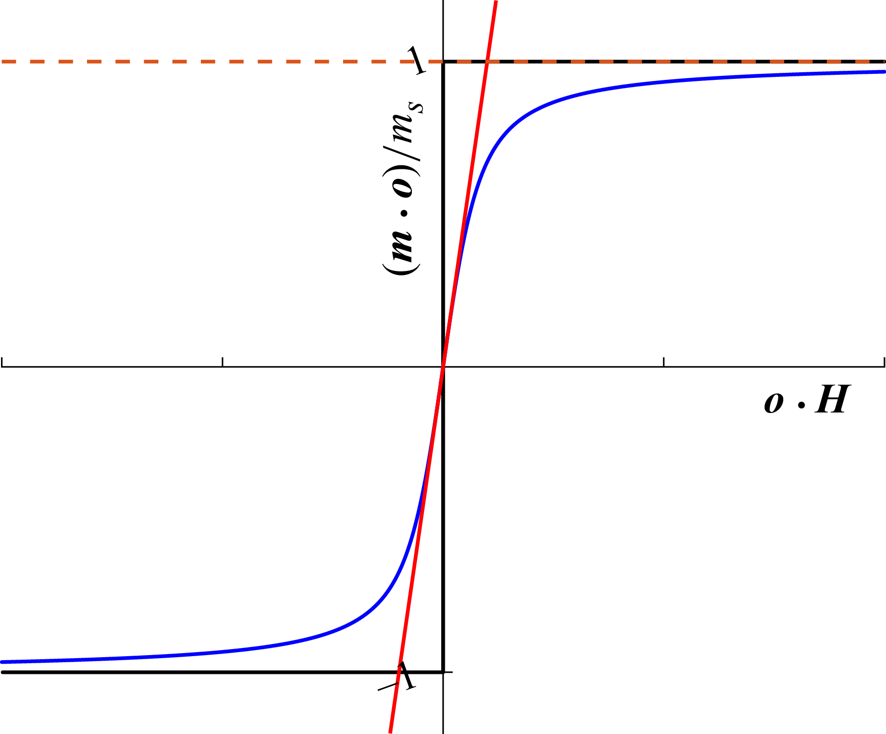
1. (i) In the permanent dipole model, $\boldsymbol{m}$ is along the orientation vector $\boldsymbol{o}$ , and the magnitude $m_s$ is a constant. This is shown by the brown dashed line in figure 2.

2. (ii) The magnitude of the moment is constant for signum model as well. The moment is along the pole of the orientation vector with positive $\boldsymbol{o} \boldsymbol{\cdot } \boldsymbol{H}$ , and there is a step change in the moment at $\boldsymbol{o} \boldsymbol{\cdot } \boldsymbol{H} = 0$ . The black line in figure 2 shows the magnetisation curve of the signum model.

3. (iii) In the linear model, $\boldsymbol{m}$ is along the orientation vector $\boldsymbol{o}$ , and the magnitude is a linear function of the component of the field along the orientation vector, $\boldsymbol{o} \boldsymbol{\cdot } \boldsymbol{H}$ , as shown by the red line in figure 2.

4. (iv) The blue line in figure 2 shows the magnitude of the moment of the Langevin model. The linear model is recovered in the limit of small magnetic field, $m_s/(\chi |\boldsymbol{H}|) \gg 1$ , and the signum model is recovered in the limit of high magnetic field, $m_s/(\chi |\boldsymbol{H}|) \ll 1$ .

Figure 2.

Magnetisation curve for non-hysteretic models: the brown dashed line - permanent dipole; black - signum; red - linear; blue - Langevin models.

For a uniform spheroidal particle, the polarisation is inclined relative to the orientation vector (Landau et al. Reference Landau, Lifshitz and Pitaevskii2014). There are components of the magnetic moment parallel and perpendicular to the orientation vector in the plane containing the orientation vector and the magnetic moment. Thus, the susceptibility has to be expressed as a tensor, containing one contribution due to the component of the magnetic field along the orientation vector which is expressed as $\chi _{\parallel } \boldsymbol{o} (\boldsymbol{o} \boldsymbol{\cdot } \boldsymbol{H})$ , and a second component due to the component of the magnetic moment perpendicular to the orientation vector, $\chi _{\perp } (\boldsymbol{I} - \boldsymbol{o} \boldsymbol{o}) \boldsymbol{\cdot } \boldsymbol{H}$ , where $\boldsymbol{I}$ is the isotropic tensor. The more general model for an anisotropic susceptibility tensor for axisymmetric particles (Samsami et al. Reference Samsami, Mirbagheri, Meshkati and Fu2020) is

(3.5) \begin{eqnarray} \boldsymbol{\chi } & = & \chi _{\parallel } \boldsymbol{o} \boldsymbol{o} + \chi _{\perp } (\boldsymbol{I} - \boldsymbol{o} \boldsymbol{o}). \end{eqnarray}

The magnetic moment is

(3.6) \begin{eqnarray} \boldsymbol{m} & = & \boldsymbol{\chi } \boldsymbol{\cdot } \boldsymbol{H} = \chi _{\parallel } \boldsymbol{o} (\boldsymbol{o} \boldsymbol{\cdot } \boldsymbol{H}) + \chi _{\perp } (\boldsymbol{I} - \boldsymbol{o} \boldsymbol{o}) \boldsymbol{\cdot } \boldsymbol{H}. \end{eqnarray}

In this model, the magnetic torque on the particle is

(3.7) \begin{eqnarray} \boldsymbol{T}^{\dagger} & = & \mu _0 (\boldsymbol{m} \times \boldsymbol{H}) = \mu _0 (\chi _{\parallel } - \chi _{\perp }) (\boldsymbol{o} \boldsymbol{\cdot } \boldsymbol{H}) (\boldsymbol{o} \times \boldsymbol{H}). \end{eqnarray}

Thus, the torque reduces to the same form as that for the scalar susceptibility in (3.3), but with an effective susceptibility $\chi _{\parallel } - \chi _{\perp }$ .

3.2. Hysteretic model

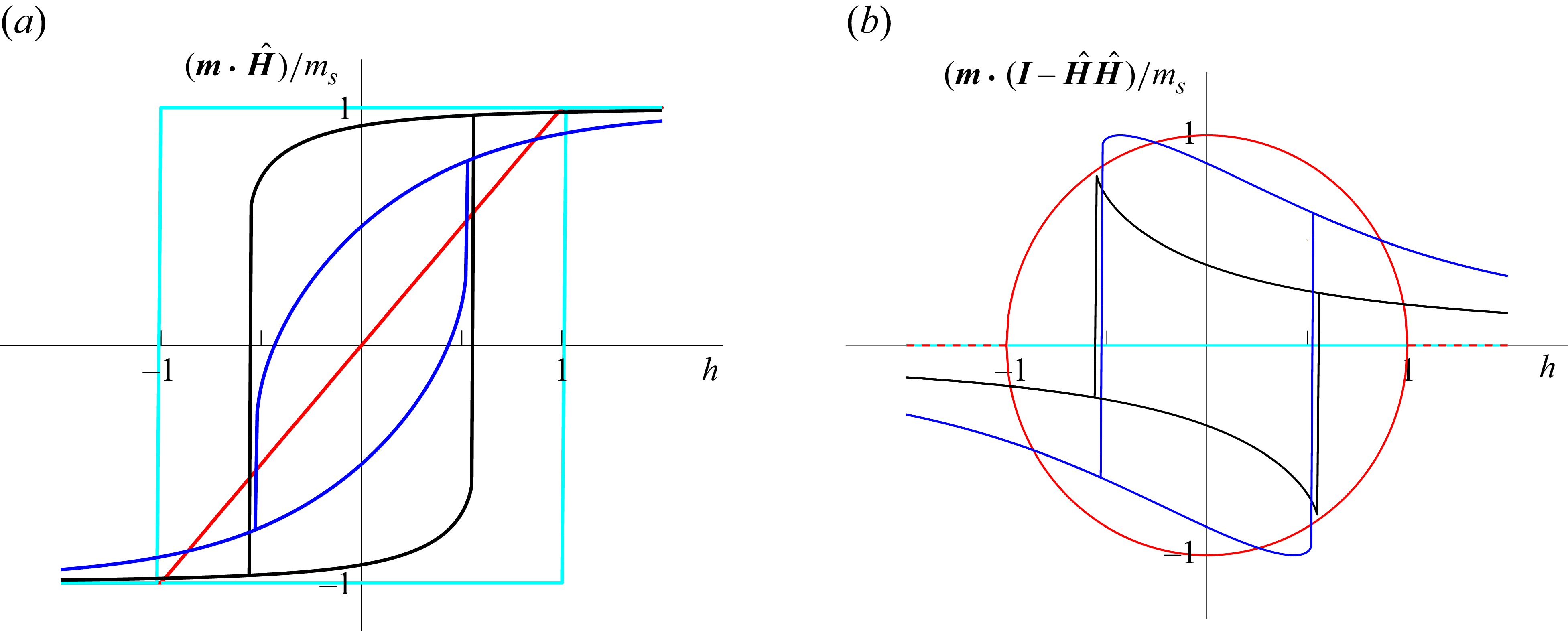
The magnetisation curve for the SW model is given by figure 3. The magnitude of the moment is a constant, $|\boldsymbol{m}| = m_s$ , but the moment orientation $\boldsymbol{m}$ makes an angle $\alpha$ with the orientation vector $\boldsymbol{o}$ in the $\boldsymbol{o} {-} \boldsymbol{H}$ plane. The angle $\alpha$ is determined from the energy minimisation conditions. The total energy is defined as

(3.8) \begin{eqnarray} E & = & - \mu _0 \boldsymbol{m} \boldsymbol{\cdot } \boldsymbol{H} + K \sin {(\alpha )}^2. \end{eqnarray}

Here, the first term is the Zeeman energy which is the potential energy of a magnetic particle in a magnetic field, and the second term is the energy penalty when the magnetic moment is not collinear with the particle orientation. The angle $\alpha$ is determined from the conditions that that the energy is a minimum with respect to variations in $\alpha$ ,

(3.9) \begin{align} \left (\frac {\partial E}{\partial \alpha } \right ) & = \sin {(\alpha )} \cos {(\alpha )} + h \sin {(\phi _H + \alpha )} = 0, \\[-12pt] \nonumber \end{align}

(3.10) \begin{align} \left (\frac {\partial ^2 E}{\partial \alpha ^2} \right ) & = \cos {(2 \alpha )} + h \cos {(\phi _H + \alpha )} \geqslant 0. \\[9pt] \nonumber \end{align}

Here, the dimensionless parameter $h = \mu _0 m_s\! H/(2K)$ is the ratio of the characteristic Zeeman and anisotropy energies.

Figure 3.

Component of particle moment parallel to field (a) and perpendicular to the field (b), obtained by solving (3.9) and (3.10), for different angles between the particle and the field for the SW model, $\phi _H = \pi /2$ (red), $\phi _H = \pi /3$ (blue), $\phi _H = \pi /8$ (black) and $\phi _H = 0$ (cyan).

Initially, the orientation angle is located at the lowest energy (i.e. (3.8)) and continues to stay at the same energy minimum. Switching takes place when there is a change in sign of the left-hand side of (3.10), the local minimum becomes a local maximum, and the system transitions to the other minimum. The switching field is the magnitude of the magnetic field at which the orientation of the magnetic moment transitions from one energy minimum to the other. Physically, it is associated with the discontinuous change of the moment orientation from close to one pole of the orientation vector to the other. Since the two energy minima correspond to orientations close to the two opposite poles of the orientation vector, the moment orientation can switch discontinuously from an orientation close to one pole of the orientation vector to the other. The value for the dimensionless switching field $h_s$ is found from (3.9) and (3.10) where the inequality is replaced by an equality,

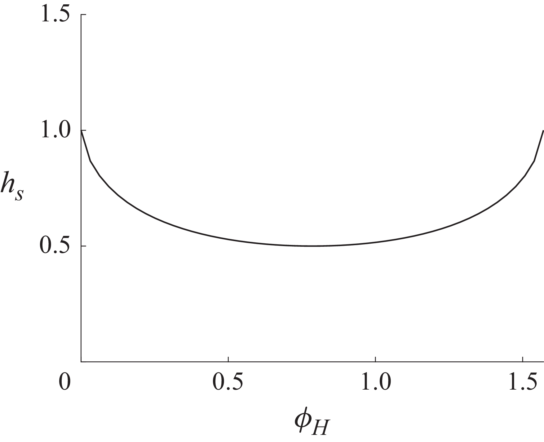
(3.11) \begin{eqnarray} h_s = \frac {1}{(\sin {(\phi _H)}^{2/3} + \cos {(\phi _H)}^{2/3})^{3/2}}. \end{eqnarray}

The variation of $h_s$ with $\phi _H$ (angle between the magnetic field and orientation) is shown in figure 4. The variations in the components of the magnetic moment parallel to the field, $\boldsymbol{m} \boldsymbol{\cdot } \kern1pt \hat {\boldsymbol{\kern-1pt H}}$ , and perpendicular to the field, $(\boldsymbol{I} - \kern1pt \hat {\boldsymbol{\kern-1pt H}} \kern1pt\! \hat {\boldsymbol{\kern-1pt H}}) \boldsymbol{\cdot } \boldsymbol{m}$ , are shown in figure 3 for different values of $\phi _H$ . Switching occurs along the vertical lines in figure 3. At these lines, one of the minima in the free energy (3.8) disappears, and the system transitions instantaneously to the other minimum. Figure 4 shows that there is no switching for $h\lt 0.5$ for any value of $\phi _H$ ; this is consistent with figure 3, where there are no vertical lines for $h\lt 0.5$ . For $0.5 \lt h \lt 1$ , switching occurs only if $\phi _H$ and $h$ are related by (3.11). For $h \gt 1$ , both figures 3 and 4 show that there is no switching. Further detail regarding the switching field is provided in Misra & Kumaran (Reference Misra and Kumaran2024a ).

Figure 4.

Variation of $h$ corresponding to switching $(h_s)$ with the angle between the orientation and the field $(\phi _H)$ .

The magnetic moments, (3.1)–(3.4), and the solution for $\alpha$ from (3.9)–(3.10), are substituted in the evolution (2.24)–(2.25) or (2.28)–(2.29), and solved to obtain the time evolution of the orientation angles.

4. One-parameter models

The only parameter in the one-parameter models is the ratio of the frequency of rotation of the magnetic field and the viscous relaxation rate of the particle, $\omega ^{\dagger}$ . For small field frequencies, the particle corotates with angular velocity equal to the field frequency, since the viscous relaxation time scale, $(A_\perp /(\mu _0 m\! H))$ or $(A_\perp /(\mu _0 \chi\! H^2))$ , is smaller than the field time period of the order $(\omega )^{-1}$ . When the field frequency increases, the viscous relaxation time scale becomes larger than the field time period. This causes the particle to ‘slip’, as the average particle angular velocity is smaller than the field angular velocity. The scaled breakdown frequency for the transition between corotating and slipping trajectories is denoted $\omega _b^{\dagger}$ .

The dynamics of a spheroid in a rotating magnetic field can be mapped onto the dynamics of a spherical particles in a steady magnetic field subject to a linear shear flow, discussed in Kumaran (Reference Kumaran2020). The equations for the azimuthal and meridional angles in a spherical coordinate are modifications of equations (3) and (4) in Kumaran (Reference Kumaran2020) when the steady magnetic field and the imposed linear shear are coplanar,

(4.1) \begin{align} \frac {\mathrm{d} \theta }{\mathrm{d} t} & = \frac {m\! H}{A_\perp } \cos {(\theta )} \cos {(\phi )}, \\[-12pt] \nonumber \end{align}

(4.2) \begin{align} \frac {\mathrm{d} \phi }{\mathrm{d} t} & = - \frac {\dot {\gamma }}{2} - \frac {m\! H}{A_\perp } \csc {(\theta )} \sin {(\phi )}, \\[9pt] \nonumber \end{align}

Here, $\dot {\gamma }$ is the imposed strain rate, and the shape factor $B$ in equations (3) and (4) in Kumaran (Reference Kumaran2020) is set equal to zero for spherical particles.

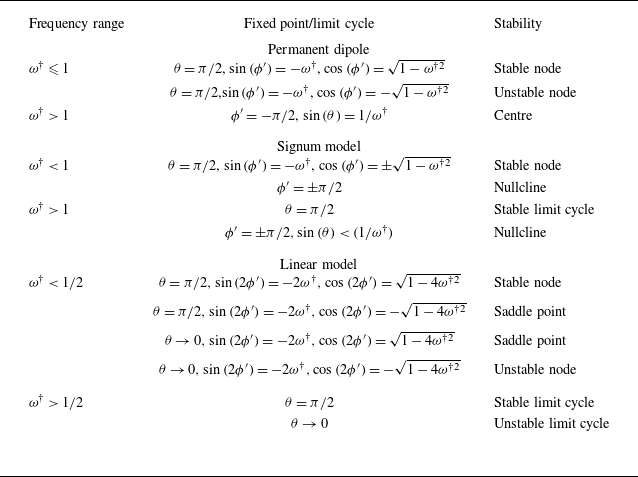
It is evident that (4.1)–(4.2) can be mapped onto the dimensional equivalents of (2.28)–(2.29) by the transformation $( {1}/{2} )\dot {\gamma } \rightarrow \omega$ . Therefore, the equations for a magnetic spheroid subject to a rotating magnetic field are identical in form to those of a spherical particle in a linear shear flow subject to a steady magnetic field in the plane of shear. Based on this transformation, the results for the present configuration can be directly obtained from those for a spherical magnetic particle in a linear shear flow and a steady magnetic field. Though the dynamics of one-parameter models have been examined in the latter configuration (Kumaran Reference Kumaran2020), the results for realistic two-parameter models are studied here. The orientation dynamics for the different one-parameter models in terms of the scaled frequency is summarised in table 1. The phase portraits and the analytical solutions for the fixed points and limit cycles are summarised in Appendix A.

Table 1.

The fixed points and the limit cycles for a magnetic particle in a rotating frame for the permanent dipole model, the induced dipole: signum model and linear model.

The particle torque is determined from (2.30)–(2.32), and the average and root mean square torque is evaluated using (2.33) and (2.34). There are three types of orientation trajectories observed in one-parameter models, parallel corotation, parallel slip and precessed slip/corotation. For the same type of trajectory, these are found to follow common relations across different models for the magnetic moment. For parallel corotation and parallel slip, only the $Z$ component of the torque and angular velocity are non-zero, and the other two components are zero. For precessed corotation/slip, the average angular velocity is in the $Z$ direction, but there are fluctuations in the $X$ and $Y$ directions.

4.1. Parallel corotation

This type of trajectory is observed when $\omega ^{\dagger}$ is less than the precession frequency or the breakdown frequency. The magnetic field and the particle rotate with equal angular velocity around the same axis. The particle orientation lags the magnetic field, but both have the same constant angular velocity in the fixed reference frame, as shown in Movie 1 (Supplementary movies are available at https://doi.org/10.1017/jfm.2026.11360). The torque along the axis of rotation is

(4.3) \begin{eqnarray} T_{Z}^{\dagger} & = & \omega ^{\dagger} . \end{eqnarray}

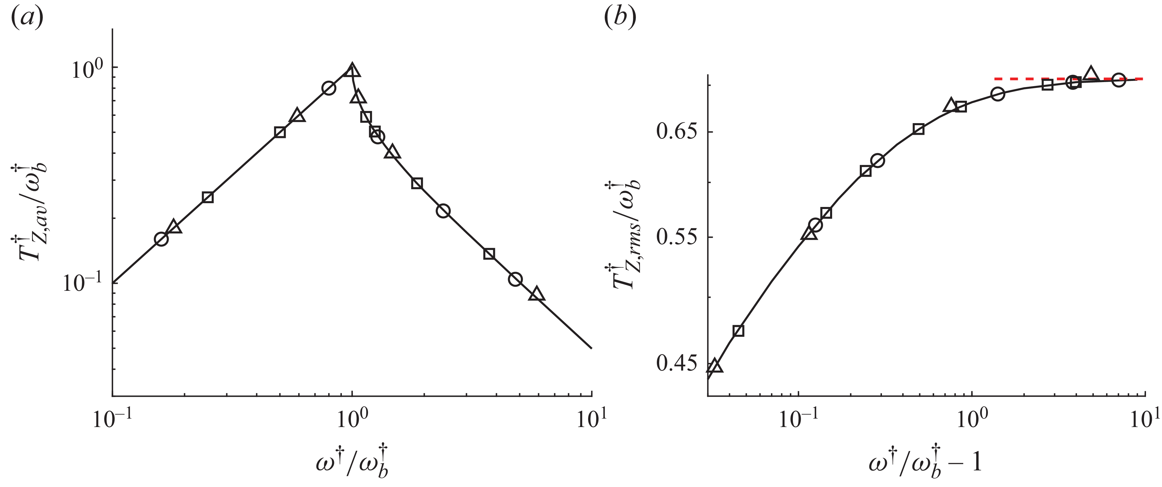
The plot of $(T_{Z,av}^{\dagger} / \omega _b^{\dagger} )$ versus $(\omega ^{\dagger} /\omega _b^{\dagger} )$ or $(T_{Z,av}^{\dagger} / \omega _p^{\dagger} )$ versus $(\omega ^{\dagger} /\omega _p^{\dagger} )$ is a straight line with slope $1$ , and $T_{Z,\textit{rms}}^{\dagger}$ is zero. This is shown by the black line with positive slope for $\omega ^{\dagger} \lt \omega _b^{\dagger}$ in figure 5(a).

Figure 5.

The scaled torques $T^{\dagger}_{Z,av}/\omega ^{\dagger} _b$ (a) and $T^{\dagger}_{Z,\textit{rms}}/\omega ^{\dagger} _b$ (b) as a function of $(\omega ^{\dagger} /\omega _b^{\dagger} )$ for the parallel corotation and parallel slip. The black line is for the linear and signum models and for the permanent dipole with parallel slip. The torque profile of SW model for $h\gt 1$ is also given by the black line. The symbols are for different values of $m_s/(\chi\! H)$ for the Langevin model, $m_s/(\chi\! H) = 8$ ( $\bigcirc$ ), $m_s/(\chi\! H) = 1$ ( $\Box$ ) and $m_s/(\chi\! H) = 0.1$ ( $\triangle$ ).

4.2. Parallel slip

For parallel slip, $\theta = \pi /2$ , the average angular velocity of the particle is smaller than that of the field, and the particle orientation has a negative angular velocity in the rotating reference frame, as shown in Movie 2. The results (A3) and (A5) for the signum and linear models can be expressed in common form when expressed in terms of the breakdown frequency $(\omega ^{\dagger} /\omega _b^{\dagger} )$ ,

(4.4) \begin{eqnarray} \frac {T^{\dagger} _{Z, av}}{\omega _b^{\dagger} } & = & \frac {\omega ^{\dagger} }{\omega _b^{\dagger} } - \sqrt { \left ( \frac {\omega ^{\dagger} }{\omega _b^{\dagger} } \right )^2 - 1}, \end{eqnarray}

where $\omega _b^{\dagger} = 1$ for the permanent dipole with $\theta = \pi /2$ and induced dipole signum model, and $\omega _b^{\dagger} = {1}/{2}$ for the induced dipole linear model. The relation (4.4) is shown by the black line with negative slope in figure 5(a).

The root mean square of the torque and angular velocity fluctuations, $T^{\dagger} _{Z,\textit{rms}}$ , are determined numerically from the solutions (A2) and (A4). The ratio $T^{\dagger} _{Z,\textit{rms}}/\omega _b^{\dagger}$ is shown as a function of $(\omega ^{\dagger} /\omega _b^{\dagger} )$ in figure 5(b). There is a common relationship for the permanent dipole and the induced dipole signum and linear models.

4.3. Precessed corotation

There is precessed corotation for the permanent dipole model when the magnetic field frequency exceeds the precession frequency $\omega _p^{\dagger} = 1$ , and the particle orientation is at the centre in figure 15(c). The particle orientation makes an oblique angle with the plane of rotation, that is, $\theta \neq \pi /2$ , but the relative angular velocity of the particle with respect to the field about the $Z$ axis is a constant, as shown in Movie 3.

The angular velocity and torque are determined by substituting (A1) for the orientation into (2.30)–(2.32),

(4.5) \begin{eqnarray} \frac {T_X^{\dagger} }{\omega _p^{\dagger} } & = & \mbox{} \pm \frac {\sqrt {\omega ^{\dagger 2} - \omega _p^{\dagger 2}} \cos {(\omega ^{\dagger} t^{\dagger} )}}{\omega ^{\dagger} }, \nonumber \\ \frac {T_Y^{\dagger} }{\omega _p^{\dagger} } & = & \mbox{} \pm \frac {\sqrt {\omega ^{\dagger 2} - \omega _p^{\dagger 2}} \sin {(\omega ^{\dagger} t^{\dagger} )}}{\omega ^{\dagger} }, \: \: \: \frac {T_Z^{\dagger} }{\omega _p^{\dagger} } = \frac {\omega _p^{\dagger} }{\omega ^{\dagger} }. \end{eqnarray}

Thus, the average torque in the $X$ and $Y$ directions are zero, and in the $Z$ direction is $(\omega _p^{\dagger 2}/\omega ^{\dagger} )$ , as shown by the black line and $ \times$ symbol in figure 6(a). The root mean square of the torque fluctuations in the $X$ and $Y$ directions is $\sqrt {(\omega ^{\dagger 2} - \omega _p^{\dagger 2})/2 \omega ^{\dagger 2}}$ , shown by the solid black lines in figure 6(b), and that in the $Z$ direction is zero.

Figure 6.

The scaled torques $T^{\dagger}_{Z,av}/\omega ^{\dagger} _p$ (a), $T_{X,rms}^{\dagger} / \omega ^{\dagger} _p = T_{Y,rms}^{\dagger} /\omega ^{\dagger} _p$ (b) and $T_{Z,\textit{rms}}^{\dagger}/\omega _p^{\dagger}$ (c) as a function of $(\omega ^{\dagger} /\omega _p^{\dagger} )$ . The black solid lines are for precessed corotation for permanent dipole where the initial orientation is at the centre in figure 15(c). The blue lines and symbols are for precessed slip for the permanent dipole with different initial conditions, $\theta _i = \pi /3, \phi _i = 3\pi /2$ $(\triangle )$ , $\theta _i = \pi /6, \phi _i = 3\pi /2$ $(\bigcirc )$ , $\theta _i = 1.5, \phi _i = \pi /3$ $(\bigtriangledown )$ , $\theta _i = 3\pi /7, \phi _i = \pi /4$ $(\diamondsuit )$ and in the plane of rotation, $\theta _i = \pi /2$ $(\Box )$ . The red dashed lines are the $(\omega ^{\dagger} /\omega _b^{\dagger} ) \gg 1$ asymptotic expressions, (4.6). The black lines with $ \times$ symbols also show the torque profiles of the SW model for $h \leqslant 1/2$ .

4.4. Precessed slip

There is precessed slip for the permanent dipole model when the particle orientation is not at the centre in the phase diagram, figure 15(c). Here, the orientation vector is not in the plane of rotation, $\theta \neq \pi /2$ , the angular velocity of the orientation vector is smaller than that of the field and the axis of rotation of the orientation vector is not collinear with that of the magnetic field. This is shown in Movie 4, where it is observed that the angular velocity of the orientation vector in the field frame is periodic, but that in the fixed frame is quasiperiodic.

The torque depends on the initial condition, that is, the specific initial orientation around the centre in figure 15(c). The torques for different initial conditions are shown by the blue lines in figure 6(a–c). In figure 6(c), the root mean square of the torque in the $Z$ direction becomes zero when the initial condition coincides with the centre (the black circle in figure 15 c), resulting in precessed corotation.

A perturbation analysis in the parameter $(\omega ^{\dagger })^{-1}$ can be used to estimate of the torque in the limit $\omega ^{\dagger} \gg 1$ , and the average torque and torque fluctuation can be found from (2.33) and (2.34),

(4.6) \begin{eqnarray} T^{\dagger }_{Z,\textit{a}v} & = & \frac {1 + \cos {(\theta _i)}^2}{{\omega }^{\dagger} }, \: \: \: T^{\dagger} _{X, \textit{rms}} = T^{\dagger} _{Y, \textit{rms}} = \frac {\cos {(\theta _i)}}{ \sqrt {2}}, \: \: \: T^{\dagger} _{Z, \textit{rms}} = \frac {\sin {(\theta _i)}}{ \sqrt {2}}. \end{eqnarray}

The above predictions, shown by the red lines on the right-hand sides of the panels in figure 6, and in good agreement with the numerical results for large $\omega ^{\dagger}$ .

5. Two-parameter models

5.1. Langevin model

The Langevin model is a non-hysteretic two-parameter model, where the parameters are the scaled frequency $\omega ^{\dagger}$ and the parameter $m_s/(\chi\! H)$ which is the ratio of the saturation moment and the susceptibility and the magnetic field. The evolution equations for the Langevin model in the rotating reference frame are (2.26), (2.27) and (3.4).

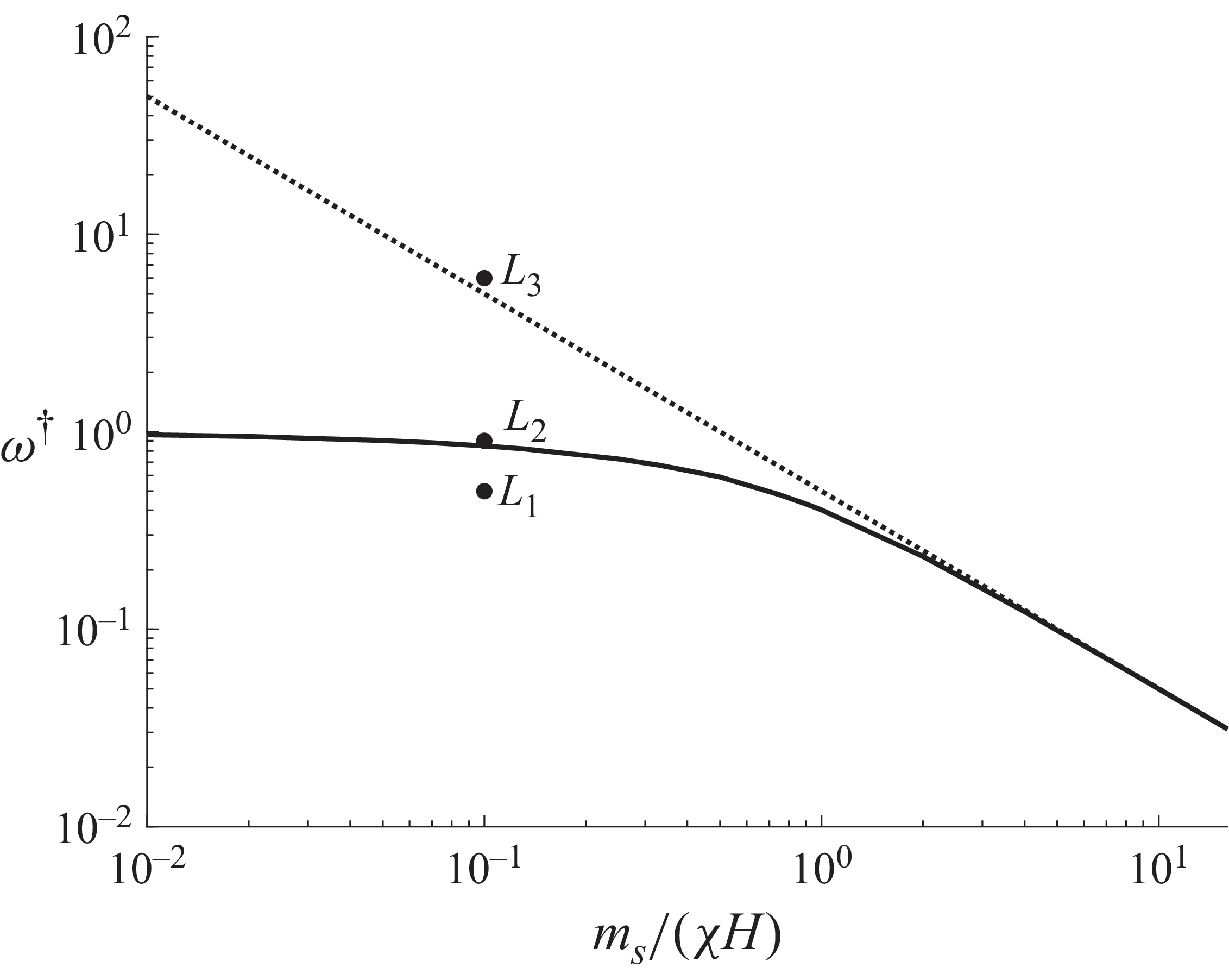
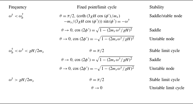
The bifurcation diagram is shown in the $m_s/(\chi\! H) {-} \omega ^{\dagger}$ plane in figure 7. There is a stable stationary point in the plane of rotation, $\theta = \pi /2$ , resulting in a parallel corotating trajectory, qualitatively similar to Movie 1, below the black line in figure 7. There is a stable rotating limit cycle, resulting in a parallel slipping trajectory qualitatively similar to Movie 2, above the black line. The fixed points and limit cycles are summarised in table 2.

Table 2.

Steady and periodic states for the Langevin model.

Figure 7.

The variation of $\omega ^{\dagger} _b$ with $(m_s/(\chi\! H))$ (solid black line), and the scaling relation $\omega ^{\dagger} = 0.5 (m_s/(\chi\! H))^{-1}$ (dashed black line).

The phase portraits at three locations in the bifurcation diagram are shown in figure 8. In this figure and the following figures, there is mirror symmetry about the vertical line $\theta = \pi /2$ between the left- and right-hand halves. Therefore, we show the standard vector plots on the left-hand sides, and the trajectories on the right-hand side, for a holistic picture of the orientation dynamics. At point $L_1$ , there is one stable node (blue circle) and one saddle point (brown circle) in the plane of rotation $\theta = \pi /2$ , and one unstable node (red circle) and a saddle (brown circle) for $\theta \rightarrow 0$ , as shown in figure 8(a). In the long time limit, there is a parallel corotating trajectory where the particle orientation tends to a fixed value shown by the blue circle in the rotating reference frame. At the black solid line in figure 7, the stable and saddle points in the plane of rotation $(\theta = \pi /2)$ merge, resulting in a stable limit cycle. At point $L_2$ above the black line in figure 7, there is one limit cycle in the plane of rotation, $\theta = \pi /2$ , resulting in a parallel slipping trajectory, as shown in figure 8(b).

Figure 8.

The particle trajectories in the $\theta {-}\phi ^{\prime}$ plane for points $L_1{-}L_3$ in figure 7 for $m_s/(\chi\! H) = 0.1$ and (a) $\omega ^{\dagger} = 0.5$ $(L_1)$ , (b) $\omega ^{\dagger} = 0.9$ $(L_2)$ and (c) $\omega ^{\dagger} = 6$ $(L_3)$ .

Since both the corotating and slipping trajectories are parallel, the breakdown frequency, which is the solid black line in figure 7, can be inferred by substituting $\theta = \pi /2$ in (2.27) and (3.4),

(5.1) \begin{eqnarray} \left [ \coth {\left ( \frac {3 \chi\! H \cos {(\phi ^{\prime} )}}{m_s} \right )} - \frac {m_s}{3 \chi\! H \cos {(\phi ^{\prime} )}} \right ] \sin {(\phi ^{\prime} )} & = & \mbox{} -\! \omega ^{\dagger} . \end{eqnarray}

Equation (5.1), which has to be solved numerically, has two solutions for $\omega ^{\dagger} \lt \omega ^{\dagger} _b$ , and no solution for $\omega ^{\dagger} \gt \omega ^{\dagger} _b$ , where $\omega ^{\dagger} _b$ is the breakdown frequency. Analytical expressions for $\omega ^{\dagger} _b$ can be derived in the limits of small and large $m_s/(\chi\! H)$ .

1. (i) For $m_s/(\chi\! H) \ll 1$ , the $\coth {}$ function in the square bracket on the left-hand side is approximately $1$ , and the second term in the square bracket is small. Equation (5.1) reduces to $\sin {(\phi ')} = \mbox{} -\! \omega ^{\dagger}$ . This approximation has a solution only for $\omega ^{\dagger} \lt 1$ . Therefore, the black boundary in figure 7 tends to $1$ for $m_s/(\chi\! H) \ll 1$ . In this limit, the Langevin model reduces to the signum model discussed in Appendix A.2, where the breakdown frequency is $\omega _b^{\dagger} = 1$ .

2. (ii) For $m_s/(\chi\! H) \gg 1$ , the term in the square bracket in (5.1) is approximately $(\chi\! H \cos {(\phi ^{\prime} )}/m_s)$ , and (5.1) reduces to $\cos {(\phi ^{\prime} )} \sin {(\phi ^{\prime} )} \chi\! H/m_s = \mbox{} -\! \omega ^{\dagger}$ . It is evident that a solution exists only for $2 \omega ^{\dagger} m_s/(\chi\! H) \lt 1$ , or $\omega ^{\dagger} \lt (\chi\! H/2 m_s)$ . This is shown by the dotted black line on the right-hand side. In this limit, the Langevin model reduces to the linear model discussed in Appendix A.3, where the breakdown frequency is $(\omega _b A_\perp /\mu _0 \chi\! H^2) = {1}/{2}$ , which is equivalent to the condition $\omega _b^{\dagger} = (\chi\! H/2 m_s)$ derived here.

A second bifurcation is observed on the black dotted line $(\omega ^{\dagger} = (\chi\! H)/(2 m_s))$ in figure 7. The saddle and unstable nodes for $\theta \rightarrow 0$ shown in figure 8(b) merge, resulting in an unstable limit cycle shown in figure 8(c) at point $L_3$ . This bifurcation does not affect the stable limit cycle in the long time limit in the plane of rotation, but it does alter the nature of the phase portrait. This bifurcation can be understood by taking the $\theta \rightarrow 0$ limit of (2.26), (2.27) and (3.4). Substituting $\cos {(\phi _H)} = \sin {(\theta )} \cos {(\phi ')} \approx \theta \cos {(\phi ')}$ (see (2.7)) in this limit, the term in the square bracket for the magnetic moment is approximated as

(5.2) \begin{eqnarray} \coth {\left (\frac {3 \chi\! H \cos {(\phi _H)}}{m_s} \right )} - \frac {m_s}{3 \chi\! H \cos {(\phi _H)}} & \approx & \frac {\chi\! H \cos {(\phi _H)}}{m_s} \nonumber \\ & \approx & \frac {\chi\! H \theta \cos {(\phi ^{\prime} )}}{m_s}. \end{eqnarray}

When this approximation is substituted into (2.26), (2.27) and (3.4), we obtain

(5.3) \begin{align} \frac {\mathrm{d} \theta }{\mathrm{d} t^{\dagger} } & = \frac {\chi\! H \theta \cos {(\phi ^{\prime} )}^2}{ m_s}, \\[-12pt] \nonumber \end{align}

(5.4) \begin{align} \frac {\mathrm{d} \phi^{\prime} }{\mathrm{d} t^{\dagger} } & = \mbox{} - \frac {\chi\! H \cos {(\phi ^{\prime} )} \sin {(\phi ^{\prime} )}}{m_s} - \omega ^{\dagger} . \\[9pt] \nonumber \end{align}

Here, we have approximated $\sin {(\theta )} \approx \theta$ and $\cos {(\theta )} \approx 1$ . Equation (5.3) indicates that $(\mathrm{d} \theta /\mathrm{d} t^{\dagger} )$ tends to zero for $\theta \rightarrow 0$ . The steady solution for $\phi '$ is $\cos {(\phi ^{\prime} )} \sin {(\phi ^{\prime} )} \chi\! H/m_s = \mbox{} -\! \omega ^{\dagger}$ . The condition for the existence of the steady solution is $\omega ^{\dagger} \lt (\chi\! H / 2 m_s)$ . When this condition is satisfied, there is one saddle point and one unstable point for orientation angles given in table 2, as explained after (5.1).

The scaled average torque ( $T^{\dagger} _{Z,av}/\omega ^{\dagger} _b$ ) and root mean square torque fluctuations ( $T^{\dagger} _{Z, \textit{rms}}/\omega ^{\dagger} _b$ ) are shown for three different values of $m_s/(\chi\! H)$ by the symbols in figures 5(a) and 5(b) for the Langevin model. These collapse onto the same curves as those for parallel corotation and slip for the permanent dipole, linear and signum models. It is important to note that though the relationship between the scaled torques and $\omega ^{\dagger} /\omega _b^{\dagger}$ is independent of $m_s/(\chi\! H)$ , the breakdown frequency $\omega _b^{\dagger}$ is a function of $m_s/(\chi\! H)$ .

5.2. The SW model

The SW model is a two-parameter model that exhibits hysteresis. The two parameters are the ratio of the magnetic field rotation rate and the viscous relaxation rate $\omega ^{\dagger}$ and the ratio of the Zeeman and anisotropy energies $h$ . Since the particle orientation and magnetic moment are not collinear in the SW model, there are different phase diagrams for the orientation and moment vectors. The physical significance of $h$ is as follows. For low $h$ , where the Zeeman energy is small compared with the anisotropy energy, the moment vector is expected to be close to the orientation vector due to the relatively large anisotropy energy penalty. For high $h$ , the anisotropy energy is relatively small; the angle between the orientation and moment vectors is expected to be large, and the phase diagrams for the orientation and moment vectors could differ.

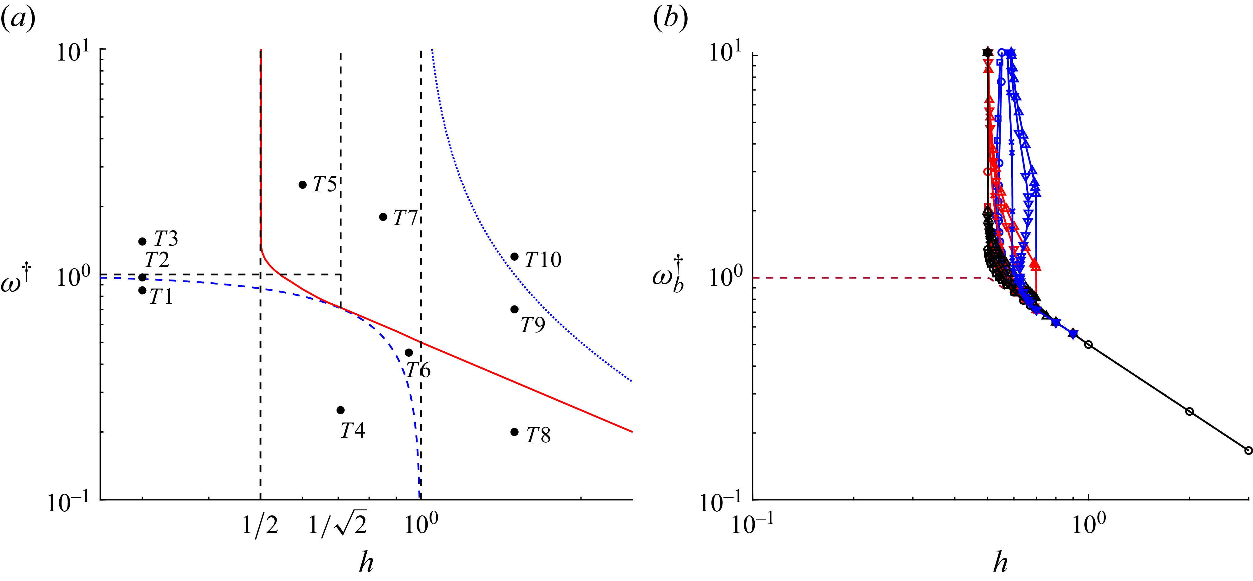
The demarcation between particle corotation and particle slip depends on the initial orientation, and there are different boundaries for different initial orientations, as shown in figure 9(b). The boundary for a particular initial condition, $\theta _i = 3\pi /8$ and $\phi ^{\prime} _i = \pi /6$ , is shown by the red line in figure 9(a). The particle corotates with the field to the left-hand side and below this line, because there is a stable fixed point for the particle orientation in the rotating reference frame. In contrast, there is a parallel slipping trajectory above and to the right-hand side of the boundary, due to a stable limit cycle for the particle orientation in the rotating reference frame. In some cases where there is slip between the particle orientation and the field, there is no slip between the magnetic field and the magnetic moment; the average angular velocity of the magnetic moment is the same as that of the magnetic field, but the moment oscillates in the plane of rotation. There is relative rotation between the magnetic moment and the orientation vector in accordance with the (3.9) and (3.10).

Figure 9.

The phase boundaries between particle corotation and particle slip in the $h{-}\omega ^{\dagger}$ plane for (a) initial condition $\theta _i = 3 \pi /8$ and $\phi _i = \pi /6$ (red line) and (b) for different initial conditions $\theta _i = 3 \pi /8$ (black lines), $\theta _i = \pi /4$ (red lines), $\theta _i = \pi /8$ (blue lines), and $\phi _i = \pi /6$ $(\bigcirc )$ , $\phi _i = \pi /3$ $(\Box )$ , $\phi _i = \pi /2$ $(\triangle )$ , $\phi _i = 2 \pi /3$ $(\bigtriangledown )$ and $\phi _i = 5 \pi /6$ $(\times )$ . Different kinds of phase portraits are observed in the regions demarcated by the dashed lines in (a), where the blue dashed line is $\omega ^{\dagger} = \sqrt {1 - h^2}$ , the dotted blue line is $\omega ^{\dagger} = 1/(2 h - 2)$ , the horizontal black dashed line is $\omega ^{\dagger} = 1$ , and the vertical black dashed lines are $h = 1/2$ , $h = 1/\sqrt {2}$ and $h = 1$ . The brown dashed line in (b) is for $\theta _i = \pi /2$ .

Though the boundary between particle corotation and slip is initial condition dependent in the region ${1}/{2} \lt h \leqslant 1/\sqrt {2}$ , the asymptotic limits of this line are $\omega ^{\dagger} _b \rightarrow \infty$ for $h = {1}/{2}$ , and $\omega ^{\dagger} _b = (1/2h)$ for $h \gt 1$ . Within these regions, there are demarcations for different types of phase portraits, labelled $T1{-}T10$ in figure 9(a). The black dashed horizontal line is the boundary $\omega ^{\dagger} = 1$ , and the black dashed vertical lines are the boundaries $h = {1}/{2}$ , $h ={1}/{\sqrt {2}}$ and $h=1$ . The blue dashed line is the boundary $\omega ^{\dagger} = \sqrt {1-h^2}$ , and the blue dotted line is the boundary $\omega ^{\dagger} = 1/(2(h-1))$ . The dependence of $\omega ^{\dagger} _b$ (equivalent of the red line in figure 9 a) for different initial conditions is shown in figure 9(b).

5.2.1. The region $h \leqslant {1}/{2}$

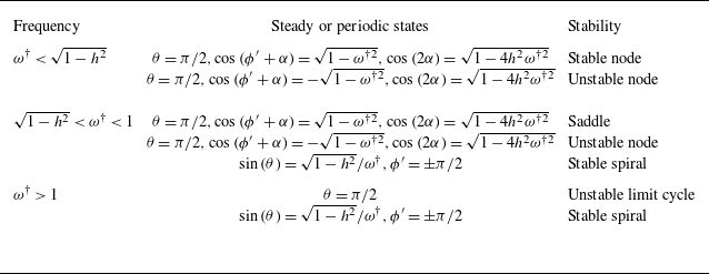
There is a transition from parallel corotation to precessed corotation for $h \leqslant {1}/{2}$ , and the precession frequency is $\omega _p^{\dagger} = \sqrt {1-h^2}$ . The phase portrait for the region $T1$ in figure 9(a), $\omega ^{\dagger} \lt \omega _p^{\dagger}$ , has one stable and one unstable node in the plane of rotation, $\theta = \pi /2$ , as shown in figure 10(a) for the particle orientation and figure 10(b) for the magnetic moment. The trajectory of the magnetic field, orientation vector and magnetic moment are shown in Movie 5. The difference from the trajectory for the one-parameter models (Movie 1) is that the particle orientation and magnetic moment are not collinear, and the magnetic moment leads the particle orientation. The solutions of (2.26), (2.27) and (3.9) are

(5.5) \begin{eqnarray} \theta & = & \pi /2, \: \: \: \sin {(\phi ' + \alpha )} = \mbox{} -\! \omega ^{\dagger} , \: \: \: \cos {(2 \alpha )} = \mbox{} \sqrt {1 - 4 h^2 {\omega ^{\dagger 2} }}. \end{eqnarray}

There is a stable node for $\cos {(\phi ' + \alpha )} = \sqrt {1 - \omega ^{\dagger 2}}$ , and an unstable node for $\cos {(\phi ' + \alpha )} = \mbox{} - \sqrt {1 - \omega ^{\dagger 2}}$ .

Figure 10.

The phase portraits for the particle orientation (a,c,e) and the magnetic moment (b,d,f) for $h=0.3$ and $\omega ^{\dagger} = 0.85$ in the region $T1$ in the $h{-}\omega ^{\dagger}$ plane in figure 9(a) (a,b); $h=0.3$ and $\omega ^{\dagger} = 0.85$ in the region $T2$ in the $h{-}\omega ^{\dagger}$ plane in figure 9(a) (c,d); $h=0.3$ and $\omega ^{\dagger} = 1.4$ in the region $T3$ in the $h{-}\omega ^{\dagger}$ plane in figure 9(a) (e,f).

At $\omega ^{\dagger} =\sqrt {1-h^2}$ , there is a crossover into region $T2$ . Here, the stable node of region $T1$ separates into a saddle point at $\theta = \pi /2$ and a stable spiral for $\theta \neq \pi /2$ in region $T2$ , as shown in figure 10(c,d). There is precession corotation for both the particle orientation and the magnetic moment, as shown in Movie 6. The two solutions of (2.26), (2.27) and (3.9) at $\theta = \pi /2$ are given by (5.5), with a saddle point for $\cos {(\phi ^{\prime} + \alpha )} = \sqrt {1 - \omega ^{\dagger 2}}$ , and an unstable node for $\cos {(\phi ^{\prime} + \alpha )} = - \sqrt {1 - \omega ^{\dagger 2}}$ . In addition, there is a stable spiral with precessed corotation for the orientation and the magnetic moment, with angles determined from (2.26), (2.27) and (3.9),

(5.6) \begin{eqnarray} \sin {(\theta )} & = & (\sqrt {1-h^2}/\omega ^{\dagger} ), \: \: \: \phi ' = - \pi /2, \: \: \: \sin {(\alpha )} = -h. \end{eqnarray}

At $\omega ^{\dagger} = 1$ , there is a crossover from region $T2$ to $T3$ , because the solutions for $\sin {(\phi ^{\prime} + \alpha )}$ in (5.5) do not exist for $\omega ^{\dagger} \gt 1$ . The saddle and unstable node at $\theta = \pi /2$ merge to form an unstable limit cycle, as shown in figure 10(e,f). There is no change in the nature of the stable spiral for $\theta \neq \pi /2$ .

The orientations of the steady and periodic states are summarised in table 3. The transitions between regions $T1$ , $T2$ and $T3$ for the SW model are modifications of the transition for a permanent dipole discussed in Appendix A.1. In the latter, the stable and unstable nodes at $\theta = \pi /2$ for $\omega ^{\dagger} \lt 1$ (figure 15 a) approach and merge at $\phi ' = - \pi /2$ for $\omega ^{\dagger} = 1$ (figure 15 b), and then separate into two centres for $\omega ^{\dagger} \gt 1$ (figure 15 c). Here, the stable node at $\theta = \pi /2$ for $\omega ^{\dagger} \lt \sqrt {1-h^2}$ first separates into a saddle point at $\theta = \pi /2$ and a stable spiral for $\theta \neq \pi /2$ for $\sqrt {1-h^2} \lt \omega ^{\dagger} \lt 1$ , and the saddle and unstable points merge to form an unstable limit cycle for $\omega ^{\dagger} \gt 1$ . This is a saddle-node bifurcation for the fixed points and an infinite period bifurcation for the limit cycle.

Table 3.

Steady and periodic states for $h \leqslant 0.5$ .

It can be shown that the SW model reduces to the permanent dipole model for $h \ll 1$ . In this limit, (3.9) is expanded in a Taylor series in $h$ to obtain

(5.7) \begin{eqnarray} \alpha & = & \mbox{} -\! h \sin {(\phi _H)} \: \: \: \mbox{or} \: \: \: \pi + h \sin {(\phi _H)}. \end{eqnarray}

There are two solutions for $\alpha$ close to the two poles of the same orientation vector, since the latter is apolar. Here, the first solution on the right-hand side is substituted into the term $\csc {(\phi _H)} \sin {(\phi _H + \alpha )}$ in (2.28) and (2.29) to obtain

(5.8) \begin{align} \csc {(\phi _H)} \sin {(\phi _H + \alpha )} & = \csc {(\phi _H)} (\sin {(\phi _H)} \cos {(\alpha )} + \cos {(\phi _H)} \sin {(\alpha )}) \nonumber \\[5pt]& = \csc {(\phi _H)}(\sin {(\phi _H)} - h \sin {(\phi _H)} \cos {(\phi _H)}) \nonumber \\[5pt]& = 1 - h \cos {(\phi _H)}. \end{align}

Therefore, in the limit $h \ll 1$ , (2.28) and (2.29) reduce to permanent dipole (2.26), (2.27), since $m^{\dagger} \rightarrow 1$ and $\alpha \rightarrow 0$ .

The stationary nodes are centres for the permanent dipole with imaginary eigenvalues $\pm \imath \sqrt {{{\omega }^{\dagger 2} } - 1}$ . There is a correction to the eigenvalues for SW model of $O(h)$ ,

(5.9) \begin{eqnarray} \lambda _1 & , & \lambda _2 = - h \pm \imath \sqrt {{{\omega }^{\dagger 2} } - 1}. \end{eqnarray}

Due to the $O(h)$ contribution to the eigenvalues, the stationary nodes are stable for the SW model for $\omega ^{\dagger} \gt 1$ .

The variation of the average and root mean square torques with $\omega ^{\dagger}$ for $h\lt {1}/{2}$ , calculated from (2.30)–(2.32). For $\omega ^{\dagger} \lt \omega _p^{\dagger}$ , where there is parallel corotation, the average torque is equal to the angular velocity of the magnetic field $\omega ^{\dagger }$ , and the root mean square of the torque fluctuations is zero. For $\omega ^{\dagger} \gt \omega _p^{\dagger}$ , there is precessed corotation, and the average torque $T_{Z,av}^{\dagger} = (1 - h^2)/\omega ^{\dagger}$ is determined from the orientation (5.6). Therefore, the scaled torque is expressed as $T_{Z,av}^{\dagger} /\omega _p^{\dagger} = (\omega _p^{\dagger} /\omega ^{\dagger} )$ , which is the same as the black line with $ \times$ symbol in figure 6(a) for precessed corotation for the permanent dipole.

Since the orientation and magnetic field corotate, there is no fluctuation in $T_Z^{\dagger}$ . In the $X$ and $Y$ directions, the average torque and mean square torque fluctuations are calculated by substituting the orientations, (5.6), into the expressions for the torque, (2.30) and (2.31), and then taking appropriate time averages. The average torques are zero, $T_{X,avg}^{\dagger } = T_{Y,avg}^{\dagger } = 0$ , and the root mean square of the torque fluctuations are $T^{\dagger} _{X, \textit{rms}} = T^{\dagger} _{Y, \textit{rms}} = \sqrt {(1 - h^2)({\omega ^{\dagger 2} } + h^2 -1)}/(\sqrt {2} \omega ^{\dagger} )$ . This can be expressed in terms of the scaled torque and the scaled rotation rate, $T^{\dagger} _{X, \textit{rms}}/\omega _p^{\dagger} = T^{\dagger} _{Y, \textit{rms}}/\omega _p^{\dagger} = \sqrt {({\omega ^{\dagger 2} } - \omega _p^{\dagger 2})}/(\sqrt {2} \omega ^{\dagger} )$ . This is the same as that for the permanent dipole with orientation at the centres, which is the black line with $ \times$ symbols in figure 6(b). Therefore, when appropriately scaled by the precession frequency, there is a common relation between the root mean square torque for the SW model for $h \leqslant {1}/{2}$ and for a permanent dipole with orientation at the centres shown by the black circle in figure 15(c). However, the precession frequency $\omega _p^{\dagger}$ does depend on the parameter $h$ .

For the special case where the initial orientation is in the plane of rotation, that is, $\theta = \pi /2$ , the final orientation is the saddle point in figures 10(c) and 10(d). In this case, there is only one transition from parallel corotation for $\omega ^{\dagger} \lt 1$ to parallel slip for $\omega ^{\dagger} \gt 1$ , that is, the breakdown frequency is $\omega ^{\dagger} _b =1$ . The orientation evolution for the magnetic field, particle and magnetic moment are shown in Movie 7. Here, the particle orientation and magnetic moment have the same angular velocity, which is lower than that of the magnetic field. In this case, the average and root mean square torques are the same as those for the one-parameter models shown by the black lines in figures 5(a) and 5(b). The average torque is $T_{Z,av}^{\dagger} = \omega ^{\dagger}$ and the root mean square of the torque fluctuations is zero for parallel corotation. For parallel slip, the average torque is $T^{\dagger} _{Z,av} = \omega ^{\dagger} - \sqrt {\omega ^{\dagger 2} - 1}$ , $T^{\dagger} _{X, \textit{rms}} = T^{\dagger} _{Y, \textit{rms}} = 0$ , and the root mean square torque is given by the black line in figure 5(b).

5.2.2. The region ${1}/{2} \lt h \lt 1$

There is the possibility of the magnetic moment switching between two minima in the free energy $E$ (see (3.8)) for ${1}/{2} \lt h \lt 1$ . This was discussed at the end of § 3.2, and this is qualitatively similar to the switching of the magnetic moment between the two poles of the orientation vector in the signum model, Appendix A.2.

The phase portraits for the region $T4$ ( ${1}/{2} \lt h \lt 1, \omega ^{\dagger } \lt \sqrt {1-h^2}$ ) are shown in figures 11(a) and 11(b) for the particle orientation and magnetic moment, respectively. The two horizontal red lines in figure 11(a) are the nullclines at $\phi ' = \pm \pi /2$ where there is a discontinuity in the angle between the orientation and magnetic moment due to switching. This is similar to the phase portrait for the signum model for $\omega ^{\dagger} \lt 1$ in figure 17(a). In addition to the nullclines, there are two stable nodes for the particle orientation with the orientation vector given by (5.5). In contrast to the phase portraits for $h\lt {1}/{2}$ in figure 10, both the nodes are stable due to the switching of the magnetic moment between the two poles of the orientation vector. There is only one stable fixed point for the magnetic moment, as shown in figure 11(b), and the two stable nodes correspond to the two poles of the same axis of the spheroid. Therefore, there is parallel corotation for the orientation vector and the magnetic moment.

Figure 11.

The phase portraits for the particle orientation (a,c,e) and the magnetic moment (b,d,f) for $h=1/\sqrt {2}$ and $\omega ^{\dagger} = 0.25$ in the region $T4$ in the $h{-}\omega ^{\dagger}$ plane in figure 9(a) (a,b); $h=0.95$ and $\omega ^{\dagger} = 0.45$ in the region $T6$ in the $h{-}\omega ^{\dagger}$ plane in figure 9(a) (c,d); $h=0.85$ and $\omega ^{\dagger} = 1.8$ in the region $T7$ in the $h{-}\omega ^{\dagger}$ plane in figure 9(a) (e,f). The blue and brown circles are stable nodes and saddles. The red dashed lines are nullclines.

The phase portraits for $\sqrt {1-h^2} \lt \omega ^{\dagger} \lt (1/2h)$ , region $T6$ in figure 9(a), are shown in figures 11(c) and 11(d). In figure 11(c) for the orientation vector, the nullclines are of finite extent, from $\sin {(\theta )} = \sqrt {1-h^2}/\omega ^{\dagger} , \phi ' = \pm \pi /2$ to $\theta = 0, \phi ' = \pm \pi /2$ , in a manner similar to that in figure 16(c) for the signum model. However, the stable node in figure 11(a) separates into a saddle and a stable node along the plane of rotation, $\theta = \pi /2$ , in figure 11(a). Here, $\cos {(2 \alpha )}$ in table 4 is positive for the stable node, and negative for the saddle node. This behaviour is in contrast to the signum model, where the transition is due to the approach of the stable node to the nullcline, as shown in figure 16(c). The magnetic moment tends towards a stable orientation in the plane of rotation, $\theta = \pi /2$ , as shown in figure 11(a). The phase portrait of the magnetic moment in this region is shown in figure 11(d), which is similar to figure 11(b). Thus, there is parallel corotation for the orientation vector and the magnetic moment, and the dynamics of the magnetic field, particle orientation and magnetic moments are qualitatively similar to those in Movie 5.

Table 4.

Steady states and limit cycles for $ {1}/{\sqrt {2}} \lt h \lt 1$ .

The phase portrait for the orientation vector for $1/\sqrt {2}\lt h\lt 1$ and $\omega ^{\dagger} \gt (1/2h)$ (region $T7$ in figure 9 a), figure 11(e), is qualitatively similar to that for the signum model for $\omega ^{\dagger} \gt 1$ (figure 16 c), where there is a nullcline of extending from $\sin {(\theta )} = \sqrt {1-h^2}/\omega ^{\dagger} , \phi ' = \pm \pi /2$ to $\theta = 0, \phi ' = \pm \pi /2$ , and there parallel slip, which is a stable limit cycle in the plane of rotation, for $\omega ^{\dagger} \gt (1/2h)$ . This is similar to that for the signum model for $\omega ^{\dagger} \gt 1$ (figure 16 c). The phase portrait for the magnetic moment, figure 11(f), is qualitatively different. In the long time limit, all initial conditions for the magnetic moment tend to a parallel oscillating state with amplitude $\sin ^{-1}{(1/(2h))}$ , as shown by the blue line in figure 11(f). The magnetic moment rotates at the same average angular velocity as the magnetic field, but there are oscillations in the moment relative to the field within one rotation. The amplitude of oscillation of the moment can be justified based on (3.9). The maximum absolute value of the first term on the left-hand side, $\sin {(\alpha )} \cos {(\alpha )}$ , is ${1}/{2}$ . As the higher order corrections for $\alpha$ increase in (5.7), the maximum value of $\sin {(2 \alpha )}$ is one. Therefore, from (3.9), the maximum magnitude of $\sin {(\phi ^{\prime} + \alpha )}$ , sine of the moment angle with the field, is $1/(2h)$ , as observed in figure 11(f). The movement of the orientation and the moment is as shown in Movie 8.

Thus, for $(1/\sqrt {2}) \lt h \lt 1$ , there is a transition between parallel corotation and parallel slip at the breakdown frequency $\omega _b^{\dagger} = (1/2h)$ . The orientation and moment angles are summarised in table 4.

For $1/2 \lt h \lt 1/\sqrt {2}$ , in the region labelled $T5$ , figure 9(b) shows that the boundary between corotating and slipping states depends on the initial orientation. This is because the nature of the final state depends on the initial condition, as shown in figures 12(a) and 12(b). For some initial conditions, the final state is the stable spiral (i.e. (5.6)) in the long time limit. Here, both the orientation and the magnetic moment corotate and precess relative to the plane of the magnetic field, as shown in figure 12(b). For other initial conditions, the orientation tends to a stable limit cycle at $\theta = \pi /2$ resulting in parallel slip, as shown in figure 12(a). The moment oscillates in the rotating reference frame, as shown in figure 12(b). The evolution of the orientation of the magnetic field, particle and magnetic moment for two different initial conditions are shown in Movie 9. Here, precessed corotation is observed for the particle orientation and magnetic field for the initial condition $\theta _i = \pi /6$ and $\phi _i = 2.18$ , but parallel slip is observed for $\theta _i = \pi /6$ and $\phi _i = 2.19$ . The switching of the magnetic moment vector between the two poles of the orientation axis is also clearly observed for parallel slip.

Figure 12.

The phase portraits for the particle orientation (a) and the magnetic moment (b) for $h=0.6$ and $\omega ^{\dagger} = 2.5$ in the region $T5$ in the $h{-}\omega ^{\dagger}$ plane in figure 9(a).

Figure 13.

Torque profile for $1/\sqrt {2}\lt h\lt 1$ and the initial conditions that lead to parallel slip for $ {1}/{2} \lt h \lt 1/\sqrt {2}$ for (a) average torque, (b) fluctuating torque. The red dotted line in (a) is the average torque profile of signum model, $(\vartriangleright )$ is for $h=0.55$ , $(\bigtriangledown )$ is for $h=0.65$ , $(\bigcirc )$ is for $h=0.75$ , $(\Box )$ is for $h=0.85$ and $(\triangle )$ is for $h=0.95$ . The red dashed line in (b) is the $T^{\dagger} _{Z, \textit{rms}}$ profile for signum model.

The maximum extent of the moment oscillation with respect to the field is $\sin ^{-1}{(1/(2h))}$ , as in the case of region $T7$ . However, the extent of moment oscillation is such that the orientation achieves the $\phi _H$ to make the moment switch for a given $h$ (figure 4).

The variation of the torque with $\omega ^{\dagger}$ for $1/2\lt h\lt 1$ is shown in figure 13. For the parallel corotating states for $\omega ^{\dagger} \lt (1/2h)$ (regions T4 and T6 in figure 9 a), the average torque $T_{Z,av}^{\dagger}$ is equal to $\omega ^{\dagger}$ , and the fluctuating torque is zero. For $\omega ^{\dagger} \gt (1/2h)$ there is coexistence of parallel slip and precessed corotation for ${1}/{2} \lt h \lt (1/\sqrt {2})$ , and parallel slip for $(1/\sqrt {2}) \lt h \lt 1$ , as shown in figures 11(e), 11(f) and 12. For parallel slip, $(T^{\dagger} _{Z,\textit{a}v}/\omega ^{\dagger} _b)$ and $T^{\dagger} _{Z,\textit{rms}}$ do depend on $h$ , as shown in figure 13. This can be attributed to the switching of the moment for the parallel slip occurring for ${1}/{2}\lt h\lt 1$ . The red lines in figures 13(a) and 13(b) are the scaled average and root mean square torques for one-parameter models (figure 5), respectively. It is observed that $T_{Z,av}^{\dagger}$ and $T_{Z,\textit{rms}}^{\dagger}$ tend to the corresponding values for the one-parameter models as $h$ is increased.

For the precessed corotating states in the region T5 in the phase diagram in figure 9(a), the orientation angles are given by (5.6), which are the same as those in region T3. Therefore, the torques are also the same as those in region T3, and the scaled torques are shown by the black lines with $ \times$ symbols in figures 6(a) and 6(b).

Table 5.

Steady states and limit cycles for $h\gt 1$ .

5.2.3. The region $h\gt 1$

The fixed points and limit cycles for $h \gt 1$ are listed in table 5, and figure 14 shows the phase portraits in the regions $T8 - T10$ for $h\gt 1$ in the phase diagram figure 9(a). The phase portrait for the orientation vector in the region $T8$ where $\omega ^{\dagger} \lt (1/2h)$ is similar to that for the induced dipole linear model in figure 17(a). The phase portrait for the orientation vector, figure 14(a) has four fixed points, one saddle and one stable node at $\theta = \pi /2$ , and one unstable node and saddle for $\theta \rightarrow 0$ . The saddle and stable node on $\theta = \pi /2$ are given in table 5. Here, $\cos {(2 \alpha )}$ is positive for the stable node, and negative for the saddle. In the limit $\theta \rightarrow 0$ , $\phi _H = \pi /2 - \cos {(\phi ^{\prime} )} \theta$ (see (2.8)). This is substituted in the energy (3.9) and (3.10) to obtain $\alpha = 3 \pi /2 + h \cos {(\phi ^{\prime} )} \theta /(h - 1)$ . The evolution (2.28) and (2.29) then become

(5.10) \begin{align} \frac {\mathrm{d} \theta }{\mathrm{d} t^{\dagger} } & = \cos {(\phi ^{\prime} )}^2 \theta /h \rightarrow 0, \\[-12pt] \nonumber \end{align}

(5.11) \begin{align} \frac {\mathrm{d} \phi ^{\prime} }{\mathrm{d} t^{\dagger} } & = -\! \sin {(2 \phi ^{\prime} )}/(2h - 2) - \omega ^{\dagger} . \\[9pt] \nonumber \end{align}

The fixed points are at $\cos {(2 \phi ^{\prime} )} = \pm \sqrt {1 - 4(h-1)^2{\omega ^{\dagger 2} }}$ , where the positive sign corresponds to a saddle, while the negative sign corresponds to an unstable node. The phase portrait of this is shown in figure 14(a). There is one stable fixed point for the magnetic moment in figure 14(b). Thus, there is parallel corotation for the orientation vector and the magnetic moment.

Figure 14.

The phase portraits for the particle orientation (a,c,e) and the magnetic moment (b,d,f) for $h=1.5$ and $\omega ^{\dagger} = 0.2$ in the region $T8$ in the $h{-}\omega ^{\dagger}$ plane in figure 9(a) (a,b); $h=1.5$ and $\omega ^{\dagger} = 0.8$ in the region $T9$ in the $h{-}\omega ^{\dagger}$ plane in figure 9(a) (c,d); $h=1.5$ and $\omega ^{\dagger} = 1.2$ in the region $T10$ in the $h{-}\omega ^{\dagger}$ plane in figure 9(a) (e, f).

The trajectories for $\omega ^{\dagger} \gt (1/2h)$ , in the regions $T9$ and $T10$ in figure 9(a), are shown in figure 14(c–f), and the time evolution of the orientation and moment vectors relative to the magnetic field vector are shown in Movie 10. In the latter, it is observed that there is corotation between magnetic moment and the magnetic field, and slip between the magnetic field and the particle orientation. This implies that the magnetic moment rotates relative to the particle orientation. However, there is no switching of the magnetic moment between the two poles of the orientation axis for $h\gt 1$ .

In figures 14(c) and 14(e), there is a stable limit cycle for the orientation vector in the plane of rotation $\theta = \pi /2$ , indicating parallel slip between the orientation vector and the magnetic field. This is similar to the phase portrait for the linear model for $\omega ^{\dagger} \gt {1}/{2}$ , figure 17(c). In figures 14(d) and 14(f), the magnetic moment tends to an oscillating trajectory along the blue lines at $\theta = \pi /2$ in the long-time limit, with an amplitude $\sin ^{-1}{(1/(2h))}$ . The average angular velocity of the magnetic moment is the same as that of the field, but there is an oscillating motion of the moment in the rotating reference frame. Though the final state of the orientation vector in the regions $T9$ and $T10$ is a stable limit cycle, there is a difference in the phase portraits. There is an unstable node and a saddle point in the phase portrait figure 14(c) for region $T9$ $(\omega ^{\dagger} \lt 1/(2h-2))$ at $\theta \rightarrow 0$ . For $\omega ^{\dagger} \gt 1/(2h - 2)$ , region $T10$ , there is an unstable limit cycle in the phase portrait figure 14(e) for $\theta \rightarrow 0$ . This is in contrast to the evolution of the phase portrait for the linear model in figure 17(b), where the stable/unstable nodes and saddle points merge simultaneously at $\omega ^{\dagger} = {1}/{2}$ .

It can be shown that the SW model reduces to the linear model in the limit $h \gg 1$ ( $\theta = \pi /2$ can be substituted without loss of generality as the stable stationary and periodic states are in $\theta = \pi /2$ plane). In this limit, the expansion $\alpha = \alpha _0 + h^{-1} \alpha _1$ is substituted into (3.9),

(5.12) \begin{eqnarray} \phi ' + \alpha _0 & = & 0 \: \: \: \mbox{or} \: \: \: \pi , \nonumber \\ \alpha _1 & = & \sin {(\phi ')} \cos {(\phi ')}\: \: \: \mbox{or} \: \: \: \mbox{} -\! \sin {(\phi ')} \cos {(\phi ')}. \end{eqnarray}

This is substituted into the term $\csc {(\phi _H)} \sin {(\phi _H + \alpha )}$ in (2.28) and (2.29),

(5.13) \begin{eqnarray} \csc {(\phi ')} \sin {(\phi ' + \alpha )} & = & \csc {(\phi ')} \sin {(h^{-1} \sin {(\phi ')} \cos {(\phi ')})} \nonumber \\ & & \: \: \: \mbox{or} \: \: \: \csc {(\phi ')} \sin {(\pi - h^{-1} \sin {(\phi ')} \cos {(\phi ')})} \nonumber \\ & = & h^{-1} \cos {(\phi ')}. \end{eqnarray}

When this is substituted into (2.28) and (2.29), the resulting equations reduce to those for the linear model, (2.28), (2.29) and (3.3), under the transformation $\omega ^{\dagger} \rightarrow (\omega ^{\dagger} /h)$ and $t^{\dagger} \rightarrow h t^{\dagger }$ . Due to this transformation, the transition from corotation to slip takes place at $\omega ^{\dagger} = (1/2h)$ for the SW model for $h \gg 1$ , instead of $\omega ^{\dagger} = {1}/{2}$ for the linear model.

Thus, for $h\gt 1$ , there is a transition between parallel corotation for $\omega ^{\dagger} \lt \omega _b^{\dagger}$ , and parallel slip for $\omega ^{\dagger} \gt \omega _b^{\dagger}$ , where $\omega _b^{\dagger} = (2 h)^{-1}$ . The scaled average and root mean square torques are same as that of the one-parameter model torques shown by the black solid lines in figures 5(a) and 5(b). These are independent of $h$ , though the breakdown frequency depends on $h$ .

6. Summary

The orientation dynamics of a spheroidal magnetic particle in a rotating magnetic field has been analysed for realistic non-hysteretic and hysteretic two-parameter models for the particle magnetic moment. In both cases, one of the parameters, $\omega ^{\dagger}$ , is the ratio of the rotation frequency of the magnetic field and the viscous relaxation rate of the particle. Superparamagnetic materials are modelled using the non-hysteretic Langevin model, where the second parameter $(m_s/\chi\! H)$ is the ratio of the saturation magnetic moment and the susceptibility times the magnetic field. Here, there is a transition from the linear variation of the moment at low magnetic field to a constant moment at high magnetic field. Ferromagnetic materials are modelled using the hysteretic SW model, where the second parameter is $h$ , the ratio of the Zeeman energy and the anisotropy energy due to the misalignment of the magnetic moment and the particle axis. In this model, there is the possibility of the moment changing discontinuously (switching) between the two poles of the orientation axis for ${1}/{2} \lt h \lt 1$ , resulting in a discontinuous change in the torque on the particle. Here, it is assumed that the dynamical time scales are much larger than the Neel relaxation time of the magnetic moment.

The results for the two parameter models are understood in the context of idealised one-parameter models, where $\omega ^{\dagger}$ is the only parameter. In the permanent dipole model, the magnetic moment is of constant magnitude and aligned towards one pole of the orientation axis independent of the magnetic field. In the linear induced dipole model, the magnitude of the magnetic moment is proportional to the component of the magnetic field along the orientation vector. In the signum induced dipole model, the magnetic moment is a constant, but the alignment is along the pole of the orientation vector which has a positive dot product with the magnetic field. In this case, there is a discontinuous switching of the magnetic moment when the orientation crosses the plane perpendicular to the magnetic field.

For the non-hysteretic Langevin model, there is a transition between two states. When $\omega ^{\dagger}$ is smaller than the breakdown frequency $\omega _b^{\dagger}$ , the angular velocity and axis of rotation of the particle is the same as that of the field – this is termed the parallel corotating state. For $\omega ^{\dagger} \gt \omega _b^{\dagger}$ , the particle angular velocity is lower than that of the field, but the axis of rotation is the same – this is termed the parallel slipping state. The breakdown frequency $\omega _b^{\dagger}$ depends on the parameter $(m_s/\chi\! H)$ ; for $(m_s/\chi\! H) \ll 1$ , the breakdown frequency tends to that for the signum model, $\omega _b^{\dagger} \rightarrow 1$ , and for $(m_s/\chi\! H) \gg 1$ , the breakdown frequency tends to that for the linear model, $\omega _b^{\dagger} \rightarrow ({1}/{2}) (m_s/\chi\! H)^{-1}$ .

Since the particle rotation axis is parallel to the $Z$ axis of rotation of the magnetic field, the components of the torque $T_X$ and $T_Y$ are zero. For the Langevin model, it is found that the average torque and the root mean square of the torque fluctuations can be mapped onto those for the linear and signum models, and the permanent dipole with $\theta _i = \pi /2$ . When $T_{Z,av}^{\dagger} /\omega _b^{\dagger}$ and $T_{Z,\textit{rms}}^{\dagger} /\omega _b^{\dagger}$ are plotted as function of $\omega ^{\dagger} /\omega _b^{\dagger}$ , these follow a universal relationship for the Langevin model, the signum model and the linear model, and the permanent dipole with $\theta _i = \pi /2$ . The expressions (4.3) and (4.4) apply for all three models.

Figure 15.

The particle trajectories in the $\theta$ and $\phi ^{\prime}$ plane for ${\omega }^{\dagger} =$ (a) $0.5$ , (b) $1$ and (c) $2$ . The blue and red $(\bigcirc )$ in (a) represent the stable and unstable nodes, respectively. The black $(\bigcirc )$ in (b) represents a higher-order fixed point and the black $(\bigcirc )$ in represent centres.

The phase portraits are more complex for the hysteretic SW model, due to the possibility of switching of the magnetic moment, as shown by previous work by Cımurs & Cēbers (Reference Cımurs and Cēbers2013) and Cēbers (Reference Cēbers2023). Here, we have used a dynamical systems approach to obtain phase portraits for the SW model for both the orientation vector and the magnetic moment. The different types of bifurcations have been identified, and these are understood in terms of the transitions for simpler one-parameter models, the linear and the signum models. The particle torque is also calculated, and it is shown that a universal relation exists between the scaled torque and the ratio of the frequency and breakdown frequency, with the exception of the parameter regime $1/2 \lt h \lt 1$ .

1. (i) For $h \gt 1$ , there is a transition at $\omega _b^{\dagger} = (2 h)^{-1}$ from parallel corotation for $\omega ^{\dagger} \lt \omega _b^{\dagger}$ to parallel slip for $\omega ^{\dagger} \gt \omega _b^{\dagger}$ . The average and root mean square torques have the same relationship as those for the signum, linear and Langevin models when both are scaled by $\omega _b^{\dagger}$ , and the relations (4.3) and (4.4) apply.

2. (ii) For $1/\sqrt {2} \lt h \lt 1$ , there is transition between parallel corotation for $\omega ^{\dagger} \lt \omega _b^{\dagger}$ to parallel slip for $\omega ^{\dagger} \gt \omega _b^{\dagger}$ , where $\omega _b^{\dagger} = (1/2h)$ . In contrast to the parallel slip for $h \gt 1$ in item (i), we find that the relation between scaled torque and $(\omega ^{\dagger} /\omega _b^{\dagger} )$ does depend on $h$ for $1/\sqrt {2} \lt h \lt 1$ .

3. (iii) For ${1}/{2} \lt h \lt (1/\sqrt {2})$ , there is parallel corotation for $\omega ^{\dagger} \lt \sqrt {1-h^2}$ , and coexistence between parallel slip and precessed corotation for $\omega ^{\dagger} \gt \sqrt {1-h^2}$ . For parallel slip, the relation between the scaled torques and the scaled frequency does depend on $h$ . For precessed corotation, there is a universal relation between the scaled torque and the scaled angular velocity, which is the same as that shown in figure 6 when the orientation is at the centre for a permanent dipole in the phase portrait in figure 15(c).

4. (iv) For $h \lt {1}/{2}$ , there is a transition at $\omega _p^{\dagger} = \sqrt {1-h^2}$ . There is parallel corotation of the orientation vector for $\omega ^{\dagger} \lt \omega _p^{\dagger}$ , and precessed corotation of the orientation vector for $\omega ^{\dagger} \gt \omega _p^{\dagger}$ . In the latter, the orientation vector is inclined relative to the plane of rotation of the magnetic field. This appears qualitatively similar to the transition for a permanent dipole, where there is a parallel corotating state for $\omega ^{\dagger} \lt 1$ and a precessed slipping state for $\omega ^{\dagger} \gt 1$ . However, there is an important difference – the centre for a permanent dipole (figure 15 c) becomes a stable spiral for the SW model (figure 10 c–e) due to the effect of hysteresis. This results in a solution for the orientation in the rotating reference frame that is independent of initial condition. The expression (4.3) applies for the parallel corotating state for the SW model for $\omega ^{\dagger} \lt \omega _p^{\dagger}$ . For the precessed corotating state, the average torque is in the $Z$ direction along the axis of the magnetic field, but there are torque fluctuations in the $X$ and $Y$ directions because the orientation is inclined relative to the plane of the field. The scaled average torque, $T_{Z,av}^{\dagger} /\omega _p^{\dagger}$ , and torque fluctuations $T_{X,rms}^{\dagger} /\omega _p^{\dagger} = T_{Y,rms}^{\dagger} /\omega _p^{\dagger}$ , collapse onto common curves when plotted against $\omega ^{\dagger} /\omega _p^{\dagger}$ . These curves are also the same as those for the permanent dipole model, when the particle orientation is located on the centre shown in figure 15(c), and the torques are given in (4.5).

It is difficult to make a quantitative comparison with experiments because not all the magnetic and hydrodynamic properties of the system are reported. In future experimental studies on rotating magnetic fields, it is necessary to determine all of the parameters that specify the magnetic properties, the fluid viscosity and the dimensions of the particle accurately, in order to make a quantitative comparison between theory and experiments. However, the qualitative nature of the dynamics determined here can be compared with previous experimental studies.

The qualitative nature of the orientation dynamics predicted here has been observed in some experimental studies. The distinction between parallel corotation and parallel slip is well known, and the torque profile shown in figure 5(a) ( $T^{\dagger} _{Z, av}/\omega ^{\dagger} _b$ versus $\omega ^{\dagger} /\omega ^{\dagger} _b$ ) is well established in the literature for different types of magnetic spheroids (McNaughton et al. Reference McNaughton, Kehbein, Anker and Kopelman2006, Janssen et al. Reference Janssen, Schellekens, van Ommering, van IJzendoorn and Prins2009). For the Langevin model, the breakdown frequency variation predicted in the limits of low and high frequency (figure 7) have been observed in experiments by Janssen et al. (Reference Janssen, Schellekens, van Ommering, van IJzendoorn and Prins2009). Here, they found that the breakdown frequency increases proportional to the field for low frequency, and proportional to the square of the field for high frequency. The low frequency limit corresponds to $(m_s/\chi\! H) \ll 1$ in figure 7, where the scaled frequency tends to a constant value, which implies that the dimensional frequency increases proportional to $H$ . The high frequency measurements correspond to $(m_s/\chi\! H) \gg 1$ , where figure 7 shows that $\omega _b^{\dagger} \propto (\chi\! H/m_s)$ , or $\omega _b \propto H^2$ . Thus, the difference in scaling of the breakdown frequency observed by Janssen et al. (Reference Janssen, Schellekens, van Ommering, van IJzendoorn and Prins2009) is predicted by the analysis of the Langevin model.

Precessed corotation and slip are reported for a particle with a finite coupling energy between the orientation and field by Cımurs & Cēbers (Reference Cımurs and Cēbers2013), and it is reported that precessed corotation is stable for field strengths below a critical value. Precessed corotation and precessed slip are known for a spherical particle subject to a steady magnetic field in shear flow in Kumaran (Reference Kumaran2020). Using the mapping between a particle in a rotating magnetic field and a sphere in a steady field subject to shear flow, this same behaviour is expected for a permanent dipole in a rotating magnetic field when the scaled rotation rate exceeds $1$ . This is discussed in Appendix A.1, where it is shown that there is a saddle-node bifurcation followed by a pitchfork bifurcation. Precessed rotation has also been seen in experiments by, for example, Ghosh et al. (Reference Ghosh, Mandal, Karmakar and Ghosh2013) and Palkar et al. (Reference Palkar, Aprelev, Salamatin, Brasovs, Kuksenok and Kornev2019). Figure 2 of Ghosh et al. (Reference Ghosh, Mandal, Karmakar and Ghosh2013) shows an experimental transition between parallel corotation (there called tumbling) and precessed corotation (there called precession). Similarly, Palkar et al. (Reference Palkar, Aprelev, Salamatin, Brasovs, Kuksenok and Kornev2019) report precessed corotation for magnetic nanorods in experiments, though there it is ascribed to a bias field.

The parameters in the two-parameter models have been determined experimentally in previous studies. Rehberg et al. (Reference Rehberg, Richter, Hartung, Lucht, Hankiewicz and Friedrich2019) measured the parameters in the Langevin model for polydisperse ferrofluids. Sampaio da Silva, Castro & de Campos (Reference Sampaio da Silva, Castro and de Campos2013) have measured the parameters in the SW model experimentally, and Durhuus, Beleggia & Frandsen (Reference Durhuus, Beleggia and Frandsen2024) have done theoretical and experimental studies on the branch-crossing in the SW model. Therefore, the parameters in these models can be measured experimentally. Using these model parameters, the present comprehensive analysis of the dynamics and torques in different regimes can be used for process design in mixing and microrheology applications. The frequency and the magnetic field magnitude can be selected so that there is parallel corotation, parallel slip or precessed corotation, and the particle angular velocities and torque can be predicted for each state. The analysis reveals a fundamental difference between superparamagnetic (Langevin model) and ferromagnetic (SW model) particles – whereas the former exhibits parallel corotating and parallel slip, the latter also has precessed corotating states for relatively small $h$ and large $\omega ^{\dagger}$ .

At the beginning of § 4, it was shown that the present configuration can be mapped onto that of a spherical magnetic particle in a shear flow and a steady magnetic field. Therefore, the present results can also be used for the latter configuration.

The analysis in § 5.2 reveals the existence of novel rotating states for $h\gt 1$ where the particle orientation slips relative to the field, but the magnetic moment corotates. This is observed in the regions T5, T7, T9 and T10 in the phase diagram figure 9(a). The possibility of different dynamics for the orientation and magnetic moment is important to consider when interpreting the results in, for example, microrheology measurements.

An important finding is the coexistence of corotating and slipping states for the SW model shown in figure 12(a). This implies that for the same magnetic field, particles with different initial orientations could exhibit different trajectories. This could provide new protocols for measurements in microrheology applications, for example, where different local rheological parameters could be simultaneously measured by following the trajectories of particles with different initial conditions driven by the same field.