1. Introduction
One of the fundamental problems in classical fluid dynamics is the Taylor–Couette flow. Even though it was formulated more than a century ago, it still intrigues researchers. The initial conception of the problem corresponds to the flow of a fluid that fills the gap between differentially rotating cylinders. The case of concentric spheres, referred to as the spherical Couette (SC) flow (Marcus & Tuckerman Reference Marcus and Tuckerman1987a,Reference Marcus and Tuckermanb), has received less attention. The main goal of investigations addressing the SC flow is to understand several aspects related to geophysical flows (Le Bars et al. Reference Le Bars, Barik, Burmann, Lathrop, Noir, Schaeffer and Triana2021), given its similarity to the Earth's geometry. In the simplest case, the SC flow is determined by the Reynolds number and the radius ratio.
The flow becomes magnetohydrodynamic (MHD) if the fluid is electrically conducting and the system is immersed in a magnetic field, which can be externally applied or auto-excited. The interaction of the shear-driven flow and the magnetic field induces electric currents. The interaction of these electric currents with the magnetic field gives rise to the Lorentz force (also referred to as the Laplace force; Avalos-Zúñiga & Rivero Reference Avalos-Zúñiga and Rivero2022), which affects the flow. Despite the non-magnetic nature of the fluid, this flow is commonly known as the magnetized spherical Couette (MSC) flow (Figueroa et al. Reference Figueroa, Schaeffer, Nataf and Schmitt2013), first addressed by Hollerbach (Reference Hollerbach1994). MHD-induced effects are possible only in working fluids of high electrical conductivity, for instance, liquid metals such as Galinstan or liquid sodium (Hollerbach et al. Reference Hollerbach, Wei, Noir and Jackson2013). The interplay of viscous, inertial and induced electromagnetic forces gives rise to a wide variety of phenomena, such as periodic rotating waves (Garcia & Stefani Reference Garcia and Stefani2018; Garcia et al. Reference Garcia, Seilmayer, Giesecke and Stefani2020; Ogbonna et al. Reference Ogbonna, Garcia, Gundrum, Seilmayer and Stefani2020), modulated rotating waves (Garcia et al. Reference Garcia, Seilmayer, Giesecke and Stefani2019, Reference Garcia, Seilmayer, Giesecke and Stefani2020), or super- and counter-rotating jets and vortices (Hollerbach Reference Hollerbach2001; Hollerbach, Canet & Fournier Reference Hollerbach, Canet and Fournier2007), depending on the explored conditions. Aiming to understand the dynamics in the interior of stars and planets, such as the dynamo effect (Adams et al. Reference Adams, Stone, Zimmerman and Lathrop2015), the MSC flow has been investigated numerically (Hollerbach Reference Hollerbach1994; Hollerbach & Skinner Reference Hollerbach and Skinner2001; Hollerbach et al. Reference Hollerbach, Canet and Fournier2007; Figueroa et al. Reference Figueroa, Schaeffer, Nataf and Schmitt2013; Kaplan, Nataf & Schaeffer Reference Kaplan, Nataf and Schaeffer2018), theoretically (Hollerbach Reference Hollerbach2009; Soward & Dormy Reference Soward and Dormy2010; Gissinger, Ji & Goodman Reference Gissinger, Ji and Goodman2011; Garcia et al. Reference Garcia, Seilmayer, Giesecke and Stefani2021) and experimentally (Sisan et al. Reference Sisan, Mujica, Tillotson, Huang, Dorland, Hassam, Antonsen and Lathrop2004; Schmitt et al. Reference Schmitt, Alboussière, Brito, Cardin, Gagnière, Jault and Nataf2008; Brito et al. Reference Brito, Alboussière, Cardin, Gagnière, Jault, La Rizza, Masson, Nataf and Schmitt2011; Kasprzyk et al. Reference Kasprzyk, Kaplan, Seilmayer and Stefani2017). A review of the theoretical and experimental works regarding the SC flow considering MHD effects can be found in Rüdiger, Kitchatinov & Hollerbach (Reference Rüdiger, Kitchatinov and Hollerbach2013).
Another approach to investigate electrically conductive fluid flows is the so-called electromagnetically driven (EMD) flow. The flow is driven by the Lorentz force produced by the interaction of externally applied magnetic fields and electric currents. This approach has been investigated in cylindrical configurations (Stelzer et al. Reference Stelzer, Cébron, Miralles, Vantieghem, Scarfe and Jackson2015a,Reference Stelzer, Miralles, Cébron, Noir, Vantieghem and Jacksonb) using liquid metal as the working fluid, and allows extending the investigation to other conducting liquids, such as electrolytes, in which induced MHD effects are weak and therefore usually disregarded. Thus the flow arises from the interplay of viscous force, inertial force and an imposed Lorentz force. Imposing a localized radial current also seems to fit geophysical applications. The interaction of solar winds with the magnetic field of a planet could lead to electric currents that start in the magnetosphere and flow to the planet's interior. Data from the robotic space probe Messenger, in the paper by Anderson et al. (Reference Anderson, Johnson, Korth, Slavin, Winslow, Phillips, McNutt and Solomon2014), report large-scale electric currents that may flow radially through the planet's crust, which is made of low-conductivity material, and then close laterally at depths where the electrical conductivity is much higher than at the surface. The possibility exists that these currents could travel radially to the planet's inner core as proposed in the present study, and play an important role in the dynamo action.
Investigation of EMD flows is limited. The rotational EMD flow of an electrolyte in the gap of concentric spheres has been studied experimentally and theoretically by Figueroa et al. (Reference Figueroa, Rojas, Rosales and Vázquez2016). In this configuration, the flow is driven by the interaction of a direct current (DC) injected radially at ring electrodes located at the equator and a dipolar magnetic field. The investigation focused on the steady-state flow. Nevertheless, it was concluded that the flow structure is quasi-axisymmetric for small electrical current densities, but becomes three-dimensional as the current increases. It was found that the basic laminar flow loses its stability and becomes time-dependent as the inner boundary layer oscillates. This time-dependent flow is investigated in Piedra et al. (Reference Piedra, Rojas, Rivera and Figueroa2022). The authors reported a vortex breakdown structure in the polar regions, validated by experiments and theoretical results. Another investigation by Figueroa et al. (Reference Figueroa, Rivero, Núñez, Rojas and Rivera2021) addressed the EMD oscillatory flow driven by a time-dependent electric current, in which the study considered theoretical and experimental results. It is essential to highlight that the spheres remained static in these three works (Figueroa et al. Reference Figueroa, Rojas, Rosales and Vázquez2016, Reference Figueroa, Rivero, Núñez, Rojas and Rivera2021; Piedra et al. Reference Piedra, Rojas, Rivera and Figueroa2022). In Proal et al. (Reference Proal, Segura, Domínguez, Rivero and Figueroa2022), the authors investigated theoretically and numerically the differential rotation of spheres with the simultaneous effect of the Lorentz force. This work considered different configurations, including differentially rotating spheres (SC flow), pure EMD flow (only Lorentz force), and ultimately both sources acting in opposite directions. In the latter case, the counteracting forces lead to a region with a high-velocity gradient (high shearing) in the bulk of the flow, but its stability was not investigated further, which is the main aim of this work. However, the flows were analysed in a limited range of parameters, and the study focused on temporally averaged flows. Thus the temporal dynamics was not observed. In the case of electromagnetic forcing with the outer sphere rotating, the counteracting forces lead to a region with a high-velocity gradient (high shearing) in the bulk of the flow, which may lead to flow instabilities that were not further investigated. This is the main aim of the present work.
Along the research line of the novel electromagnetically driven flow in non-conductive shells proposed by Figueroa et al. (Reference Figueroa, Rojas, Rosales and Vázquez2016), this work analyses experimentally and theoretically a hydrodynamic instability in a spherical annulus promoted by an electromagnetically driven anticyclonic rotation. To the best knowledge of the authors, there is scarce experimental and theoretical evidence regarding this type of flow, which is the main aim of this work. We follow a simple experimental device (Proal et al. Reference Proal, Segura, Domínguez, Rivero and Figueroa2022), which is very flexible in terms of the spatial structure of the forcing and keeps some fundamental aspects of the flow in planetary interiors, allowing particle image velocimetry (PIV) measurements in the fluid interior. As far as the authors are aware, this is the first time that this instability has been reported in an electromagnetically driven flow between a system of concentric rotating spheres.
2. Experimental procedure
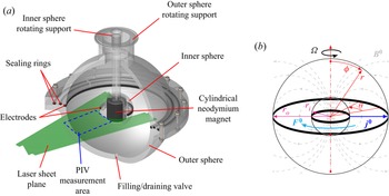
Only a brief account of the experimental set-up used in these experiments will be explained, given that there is a thorough description provided in Proal et al. (Reference Proal, Segura, Domínguez, Rivero and Figueroa2022). As seen in figure 1(a), the experiment consists of concentric Plexiglas spheres. The radii of the outer and inner spheres are  $r_o=0.105$ m and
 $r_i=0.035$ m, respectively. The radius ratio
 $r_o / r_i = 3$ matches the Earth's interior ratio. Additionally, the dimensionless gap is
 $\beta =(r_o-r_i)/r_i=2$. A weak electrolytic solution of sodium bicarbonate (NaHCO
 $_3$) at
 $8.6\,\%$ by weight fills the gap between the spheres. The mass density, kinematic viscosity and electrical conductivity of the electrolyte are
 $\rho =1090\,{\rm kg}\,{\rm m}^{-3}$,
 $\nu =10^{-6}\,{\rm m}^{2}\,{\rm s}^{-1}$ and
 $\sigma =6.36\,{\rm S}\,{\rm m}^{-1}$, respectively. A cylindrical neodymium magnet inside the hollow inner sphere generates a dipolar magnetic field. The
 $z$-axis of the magnet is aligned with the vertical gravity vector and coincides with the rotation axis. The value of the magnetic field at the equator of the inner sphere is
 $B^0_e=0.065$ T. A DC electric current is injected through two graphite ring-shaped electrodes. The width of the rings is
 $h=0.005$ m. The electrodes were located externally and internally on the equator of the internal and external spheres, respectively. The amplitude of the injected current was set to
 $I=50$ mA, which corresponds to an electric potential difference of
 $\Delta V=1.75$ V. Under these imposed conditions on the electrical variables, electrolysis did not affect the experiments. The outer sphere rotates at a constant angular velocity
 $\varOmega =0.251\,{\rm rad}\,{\rm s}^{-1}$. The electric current interacts with the non-uniform magnetic field distribution, generating a Lorentz force that sets the fluid in motion. After the transient, velocity fields were obtained experimentally with PIV. The measurements were performed 5 mm beneath the equatorial plane to prevent shadowing from the electrodes. The PIVlab software was used to perform the analysis (Thielicke & Stamhuis Reference Thielicke and Stamhuis2014). Adjusting a normal distribution to the data at the sampled points allowed us to obtain the error in the velocity data. Under these conditions, the maximum error in the experimental observations was 15 %.
An electrolytic solution fills the gap between the outer and inner spheres with radii  $r_o$ and
 $r_i$, respectively. The outer sphere rotates at constant angular speed
 $\boldsymbol {\varOmega }$. The inner sphere is at rest and encloses a cylindrical permanent magnet, which produces the imposed dipolar magnetic field
 $\boldsymbol {B}^{0}$. The DC electric current
 $\boldsymbol {j}^{0}$ is mainly radial and is injected through two copper ring electrodes located at the equator of the spheres. The main direction of the Lorentz force is denoted by
 $\boldsymbol {F}^0$. The flow is visualized in a section of the equatorial plane with PIV. (a) Three-dimensional model of the experimental set-up. (b) Physical model (not drawn to scale).

3. Statement of the problem
The simplified physical model of the present work consists of a system of two concentric spheres immersed in a dipolar magnetic field that interacts with a radial electric current density injected in the equatorial plane. This interaction generates an electromagnetic force in the azimuthal direction, as observed in figure 1(b). Additionally, the outer sphere rotates independently with a constant angular velocity around the vertical axis. The working fluid contained in the annular gap is an electrolyte. Mathematically, the continuity and Navier–Stokes equations with the Lorentz force as source term (Figueroa, Cuevas & Ramos Reference Figueroa, Cuevas and Ramos2011; Figueroa et al. Reference Figueroa, Rojas, Rosales and Vázquez2016, Reference Figueroa, Rivero, Núñez, Rojas and Rivera2021; Proal et al. Reference Proal, Segura, Domínguez, Rivero and Figueroa2022; Piedra et al. Reference Piedra, Rojas, Rivera and Figueroa2022) allow modelling electromagnetically driven flows of weak electrolytes. In this case, the low magnetic Reynolds number or quasi-static approximation is valid (Figueroa et al. Reference Figueroa, Rivero, Núñez, Rojas and Rivera2021). In the laboratory frame of reference, the dimensionless governing equations read
 \begin{gather} \boldsymbol{\nabla} \boldsymbol{\cdot} \boldsymbol{u} = 0 , \end{gather}
 \begin{gather} \dfrac{\partial \boldsymbol{u}}{\partial t} + (\boldsymbol{u} \boldsymbol{\cdot} \boldsymbol{\nabla}) \boldsymbol{u} ={-}\boldsymbol{\nabla} p + E_k'\,\nabla^2 \boldsymbol{u} + \varLambda_L' (\,\boldsymbol{j^0} \times\boldsymbol{B^0} ) , \end{gather}
with  $\boldsymbol {u}$ the velocity vector normalized by the total velocity
 $V$. The total velocity is the sum of the tangential velocity
 $U= \varOmega d$ of the rotating outer sphere with constant angular speed
 $\varOmega$ and the viscous velocity
 $u_0=\nu /d$, where
 $\nu$ is the kinematic viscosity of the fluid, and
 $d$ is the characteristic length, taken as the gap between spheres,
 $d=r_o-r_i$. The pressure field, denoted by
 $p$, is normalized by the dynamic pressure
 $\rho V^2$, where
 $\rho$ is the density of the fluid. Coordinates are normalized by
 $d$. In turn, time
 $t$ is normalized with
 $d/V$. The last term on the right-hand side of (3.2) represents the Lorentz force created by the applied electric current density
 $\boldsymbol {j}^{0}$ and magnetic field
 $\boldsymbol {B}^{0}$. The latter field distribution is modelled as a dipole:
 \begin{equation} \boldsymbol{B}^{0} = \frac{r_i^{3}}{r^{3}} (2 \cos \phi\,\hat{r} + \sin \phi\,\hat{\phi}) , \end{equation}
where the magnetic field  $\boldsymbol {B}^{0}$ is normalized by its magnitude at the equator of the inner sphere
 $B^0_e$. The co-latitude is
 $\phi$, whereas
 $\hat {r}$ and
 $\hat {\phi }$ are the unitary vectors in the radial and polar directions, respectively. Here,
 $r_i$ is the dimensionless radius of the inner sphere. As stated in Proal et al. (Reference Proal, Segura, Domínguez, Rivero and Figueroa2022), the dipolar magnetic field model, given by (3.3), is in good agreement with measurements of the magnetic field produced by the cylindrical magnet located inside the inner sphere. For ring electrodes situated at the equator, the electric current density is mainly radial, and its mathematical expression is (Figueroa et al. Reference Figueroa, Rojas, Rosales and Vázquez2016; Proal et al. Reference Proal, Segura, Domínguez, Rivero and Figueroa2022)
 \begin{equation} \boldsymbol{j}^0 = \frac{r_i^2}{r^{2}}\,\hat{r} , \end{equation}
which is normalized by the magnitude of the current density at the electrode of the inner sphere  $j^0=I/A_i$, where
 $A_i$ is the transverse area of the electrode (
 $A_i=2 {\rm \pi}r_i h$). Close to the electrode rings, there also exists a component
 $j_{\phi }$ in the polar direction with the same order of magnitude as the radial one,
 $j_r$ (Piedra et al. Reference Piedra, Rojas, Rivera and Figueroa2022). However, the electric current behaves mainly as
 $j_r \sim r^{-2}$, which allowed a good comparison with experimental velocity fields, as in previous studies (Figueroa et al. Reference Figueroa, Rojas, Rosales and Vázquez2016, Reference Figueroa, Rivero, Núñez, Rojas and Rivera2021; Proal et al. Reference Proal, Segura, Domínguez, Rivero and Figueroa2022). In this model, the spheres are electric insulators, and the electrodes are considered as perfect conductors. Thus (3.4) is valid in the domain
 $r_i \leq r \leq r_o$,
 $0 \leq \theta \leq 2{\rm \pi}$,
 $({\rm \pi} /2 -\epsilon ) \leq \phi \leq ({\rm \pi} /2 -\epsilon )$, where
 $\epsilon =h/2r_i$. The electric current outside the latter domain is set to zero. The flow dynamics are governed by two dimensionless parameters,
 $E_k'=\nu / V d$ and
 $\varLambda _L'=j^0 B^0_e d/ \rho V^{2}$. The choice for
 $V$ as the characteristic velocity arises from the fact that the system of equations (3.1)–(3.2) depicts a general model that considers the viscous, Coriolis and applied Lorentz forces. If
 $\varOmega d \ll \nu / d$, then we can obtain a previous dimensionless model where the spheres are at rest and the only forcing is the electromagnetic one (Piedra et al. Reference Piedra, Rojas, Rivera and Figueroa2022). In the present work, the rotation velocity is larger than the diffusive velocity
 $\varOmega d \gg \nu / d$; the difference is three orders of magnitude, thus
 $V \approx \varOmega d$. Under this estimate, the dimensionless numbers in (3.2) approximate the Ekman (
 $E_k' \approx E_k=\nu / \varOmega d^2$) and Elsasser (
 $\varLambda _L' \approx \varLambda _L=j^0 B^0_e / \rho \varOmega U$) numbers. Thus the flow dynamics can be described with
 $E_k$ and
 $\varLambda _L$, which denote the ratio of viscous to Coriolis forces and the ratio of Lorentz to Coriolis forces, respectively. Since the Hartmann number
 $Ha =B^0_e d \sqrt {\sigma / \rho \nu }=0.35$ is less than unity, induction effects are negligible. Equations (3.1)–(3.2), along with the expression for the magnetic field (3.3), and the current density (3.4), form a closed system for solving the electromagnetically driven flow in the gap between spheres, which was solved numerically with an in-house code, based on the finite difference method, previously described and validated with analytical and experimental data (Figueroa et al. Reference Figueroa, Rojas, Rosales and Vázquez2016, Reference Figueroa, Rivero, Núñez, Rojas and Rivera2021; Proal et al. Reference Proal, Segura, Domínguez, Rivero and Figueroa2022; Piedra et al. Reference Piedra, Rojas, Rivera and Figueroa2022). The numerical solution considers no-slip conditions on the spheres, whereas the initial conditions consider a quiescent fluid (
 $\boldsymbol {u}=0$) with no electric current (
 $\boldsymbol {j}^0=0$).
4. Main results
4.1. Mean flow
In the case of motionless spheres, the radial electric current interacts with the dipolar magnetic field generating an azimuthal Lorentz force that stirs the fluid. In the present configuration, the electromagnetically driven flow rotates in the negative  $\theta$-direction, with the maximum velocity region close to the inner sphere (Figueroa et al. Reference Figueroa, Rojas, Rosales and Vázquez2016; Proal et al. Reference Proal, Segura, Domínguez, Rivero and Figueroa2022), where both the magnetic field and the electric current are intense, and decay as
 $r^{-3}$ and
 $r^{-2}$, respectively. In turn, the Lorentz force decays as
 $r^{-5}$. Conversely, when the outer sphere rotates in the positive
 $\theta$-direction with a constant angular velocity and no current is injected, the no-slip condition directs the momentum transfer to the fluid. In this case, the flow is driven in the positive
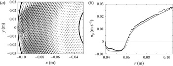
 $\theta$-direction, and the velocity reaches a maximum at the outer sphere and decays monotonically to zero at the inner sphere (Proal et al. Reference Proal, Segura, Domínguez, Rivero and Figueroa2022). When both effects are present, namely, the rotation of the outer sphere and the electromagnetic stirring, two counter-rotating flows can be observed, as seen in figure 2(a). This figure shows the time-averaged experimental observations at the equatorial plane (
 $\phi ={\rm \pi} / 2$) for current intensity
 $I=50$ mA and angular speed of the outer sphere
 $\varOmega =0.251\,{\rm rad}\,{\rm s}^{-1}$. The dynamics of the global flow depends on the interplay between the shearing due to the localized electromagnetic forcing and the rotation of the outer sphere. The interplay of the counteracting driving forces generates a stagnant region close to the inner sphere at
 $r \approx 0.06$ m, observed in figure 2(a). That is, the velocity profiles present regions with negative and positive velocities. The profile of the azimuthal velocity
 $u_{\theta }$, from the experimental velocity field, along with the three-dimensional numerical results, is shown in figure 2(b). We observe that the three-dimensional numerical solution with the experimental observations agrees quantitatively. The azimuthal velocity due to the rotation of the sphere is
 $u_{\theta } \approx 26.4\,{\rm mm}\,{\rm s}^{-1}$, and the maximum velocity due to the electromagnetic forcing is
 $u_{\theta, max} \approx 7.5\,{\rm mm}\,{\rm s}^{-1}$. Based on the Reynolds number definition, it is possible to determine the corresponding Reynolds numbers for the inner and outer flows,
 $ {\textit {Re}} _i= u_{\theta,max} r_i / \nu =260$ and
 $ {\textit {Re}} _o=\varOmega r_o^2 /\nu =2770$, respectively, which state that the flows under study are in the laminar regime.
Electromagnetic stirring and rotating external sphere. (a) Time-averaged velocity field of the flow at the equator ( $\phi ={\rm \pi} /2$); experimental PIV observation. (b) Radial profile of the azimuthal velocity
 $u_{\theta }$ as function of the
 $r$-coordinate at the equator. The markers and the continuous line denote experimental measurements and numerical results, respectively. Here,
 $E_k=8.12 \times 10^{-4}$ and
 $\varLambda _L=2.15 \times 10^{-2}$ (
 $I=50$ mA,
 $\varOmega =0.251\,{\rm rad}\,{\rm s}^{-1}$).

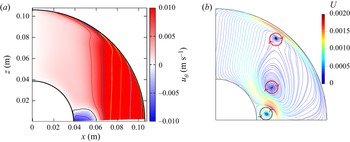
Since the numerical model is validated with the experimental data, we can use it to discern a major picture of the three-dimensional flow. Figure 3(a) shows the time-averaged azimuthal velocity ( $u_{\theta }$) map for the meridional plane. Under the time-averaged observation, the velocity map is axisymmetric and preserves symmetry with respect to the equator. Thus only a quadrant is shown for the meridian plane, where we observe the positive velocity region (cyclonic motion) in red and the negative (anticyclonic motion) region in blue. Due to the localized electromagnetic stirring, the anticyclonic motion is confined to the region close to the equator of the inner sphere. The vertical isolines in the positive velocity region denote a geostrophic motion in the cyclonic flow. Recalling the Rossby number
 $Ro=u_{\theta,max} / 2 \varOmega d=0.21$, the centrifugal force is negligible. Therefore, in this case, the balance is between the Coriolis and electromagnetic forces (or geostrophic balance). In another perspective, the Ekman number is
 $E_k=8.12 \times 10^{-4}$; thus the disturbances can propagate before decaying owing to viscous effects. Also, the Elsasser number is
 $\varLambda _L=2.15 \times 10^{-2}$, which means that the effects of rotation are large and the net accelerations small. This plot also shows that the velocity is close to zero in the polar region. Additionally, figure 3(b) shows the time-averaged meridional recirculation, where the streamlines are plotted. As in the hydrodynamic SC case in a wide gap (Tuckerman & Marcus Reference Tuckerman and Marcus1985; Hollerbach, Junk & Egbers Reference Hollerbach, Junk and Egbers2006), the total flow is symmetric to the equator and the rotation axis, and it is composed by the superposition of the azimuthal rotation and the meridional circulation. This poloidal flow is one order of magnitude smaller than the azimuthal flow. In contrast to the hydrodynamic SC case where the spheres counter-rotate (Gertsenshtein, Jilenko & Krivonosova Reference Gertsenshtein, Jilenko and Krivonosova2002) (
 $\beta =1$,
 $ {\textit {Re}} _i=500$,
 $ {\textit {Re}} _o=500$) and two poloidal vortices are observed, we can find three poloidal vortices in our case. In this case study, the electromagnetic forcing gives rise to the innermost vortex since the forcing is higher close to the equatorial region of the inner sphere. The latter is analogue to the magnetic obstacle case (Cuevas, Smolentsev & Abdou Reference Cuevas, Smolentsev and Abdou2006), where the inner vortices (or magnetic vortices) are caused by the localized magnetic field of the obstacle (Votyakov & Kassinos Reference Votyakov and Kassinos2010), creating a shear gradient in the mean flow.
Time-averaged plot at the meridional plane. The arrows denote the sense of rotation of the vortices for the streamlines. Here,  $E_k=8.12 \times 10^{-4}$ and
 $\varLambda _L=2.15 \times 10^{-2}$ (
 $I=50$ mA,
 $\varOmega =0.251\,{\rm rad}\,{\rm s}^{-1}$). Numerical simulations. (a) Azimuthal velocity
 $u_{\theta }$ map. (b) Poloidal streamlines.

4.2. Time-dependent flow
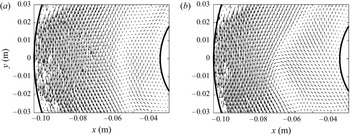
The flow dynamics turns out to be more complicated and exhibits a richer behaviour when the flow is not averaged in time. Figure 4 shows instantaneous velocity fields at the equatorial plane from the experimental PIV observations for two time instants. As discussed in § 4.1, the interplay between the rotation of the external sphere and the electromagnetically driven anticyclonic flow generates a strong shearing at the stagnant region ( $r \approx 0.06$ m under-explored conditions) that promotes an instability that triggers the appearance of translating vortices in this region, as presented in figures 4(a,b). In figure 4(a), we observe a cyclonic vortex whose centre is located at
 $x=-0.06$ m,
 $y=0$ m, and it is advected to follow a cyclonic motion, as seen in figure 4(b). However, visualization on this plane is insufficient to fully understand the flow.
Instantaneous velocity fields at the equatorial plane: (a)  $t=300$ s, (b)
 $t=307$ s. Cyclonic rotation of the instability. Here,
 $E_k=8.12 \times 10^{-4}$ and
 $\varLambda _L=2.15 \times 10^{-2}$ (
 $I=50$ mA,
 $\varOmega =0.251\,{\rm rad}\,{\rm s}^{-1}$). Experimental observations.

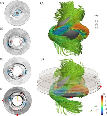
The complete structure of the instability can be visualized in figure 5, where the instantaneous streamlines are plotted for a given time instant. In figure 5(a), the streamlines are plotted in the equatorial plane. The vortex in the left part coincides with the experimental one shown in figure 4(a). We observe a total of four vortices in the high-shear region. It is noteworthy that the left and right vortices (highlighted in blue) are cyclonic, while the upper and lower vortices (highlighted in red) are anticyclonic. Figures 5(b–d) illustrate different planes parallel to the equator for  $z=0.01$,
 $0.02$ and
 $0.04$ m, respectively. These planes are shown in figures 5(e,f). From figures 5(a–d), it is possible to observe that the locations of vortices varied with the
 $z$-plane, and merge close to the poles to form a single cyclonic vortex.
Three-dimensional structure of the instability. Instantaneous streamlines plotted at the marked planes parallel to the equator: (a)  $z=0$ m, (b)
 $z=0.01$ m, (c)
 $z=0.02$ m, and (d)
 $z=0.04$ m. Instantaneous three-dimensional streamlines coloured by the angular velocity: (e) isometric view, ( f) side view. Cyclonic rotation of the instability. Here,
 $E_k=8.12 \times 10^{-4}$ and
 $\varLambda _L=2.15 \times 10^{-2}$ (
 $I=50$ mA,
 $\varOmega =0.251\,{\rm rad}\,{\rm s}^{-1}$). The arrows denote the directions of rotation of the vortices for the streamlines. The red triangle and disc are markers for mapping the position between two-dimensional and three-dimensional figures. The streamlines are coloured according to the angular velocity
 $\omega$. Numerical simulations.

Additionally, figures 5(e,f) present isometric and side views of a three-dimensional picture of the instability. The rotation of each vortex is coloured by the angular velocity, denoting that two tornado-like vortices rotate cyclonically (in blue), and two rotate anticyclonically (in red), while their intensity reduces in the polar direction. The tornadoes are equidistant from each other; they are inclined with respect to the equatorial plane (by approximately  $50^{\circ }$) and entangled in the polar direction. The anticyclonic tornadoes are more inclined,
 $-60^{\circ }$. Though not observed in figure 5, the whole flow structure propagates in the direction of rotation of the outer sphere; that is, the instability performs a cyclonic rotation, as seen in supplementary movie 1 available at https://doi.org/10.1017/jfm.2023.183. We can appreciate that the rotation of the instability is slower than the rotation of the outer sphere. Even though a similar system of helicons has been reported for the hydrodynamic SC case where the spheres counter-rotate for
 $\beta =1$,
 $ {\textit {Re}} _i=430$,
 $ {\textit {Re}} _o=900$ (Zhilenko, Krivonosova & Nikitin Reference Zhilenko, Krivonosova and Nikitin2007), only a sketch of the instability was provided by the authors. In contrast, the present work shows the full structure of the flow based on experimental and computational data.
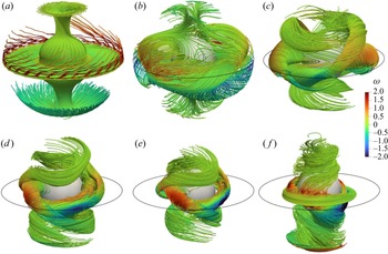
Figure 6 shows the instantaneous three-dimensional streamlines for different angular velocities of the outer sphere and a constant electromagnetic forcing. As can be observed in figure 6(a), for a low angular velocity, the flow is very similar to the basic state of the SC flow when the inner sphere rotates. As the angular velocity increases, the flow generated by the shear stress on the outer sphere becomes more intense. Its interaction with the electromagnetically driven flow close to the inner sphere triggers the instability. The four vortical structures develop close to the equatorial region and propagate vertically along the axis of rotation towards the poles (figures 6b,c). Notice that as the angular velocity of the outer sphere increases, the tornado-like vortices are reduced to the inner sphere region, as can be seen in figures 6(d–f).
Instantaneous three-dimensional streamlines: (a)  $Ro=1.7$,
 $E_k=6.5 \times 10^{-3}$,
 $\varLambda _L=1.38$ (
 $\varOmega =0.031\,{\rm rad}\,{\rm s}^{-1}$); (b)
 $Ro=0.85$,
 $E_k=3.25 \times 10^{-3}$,
 $\varLambda _L=0.345$ (
 $\varOmega =0.063\,{\rm rad}\,{\rm s}^{-1}$); (c)
 $Ro=0.426$,
 $E_k=1.62 \times 10^{-3}$,
 $\varLambda _L=8.62 \times 10^{-2}$ (
 $\varOmega =0.126\,{\rm rad}\,{\rm s}^{-1}$); (d)
 $Ro=0.284$,
 $E_k=1.08 \times 10^{-3}$,
 $\varLambda _L=3.83 \times 10^{-2}$ (
 $\varOmega =0.188\,{\rm rad}\,{\rm s}^{-1}$); (e)
 $Ro=0.213$,
 $E_k=8.12 \times 10^{-4}$,
 $\varLambda _L=2.15 \times 10^{-2}$ (
 $\varOmega =0.251\,{\rm rad}\,{\rm s}^{-1}$); ( f)
 $Ro=0.17$,
 $E_k=6.5 \times 10^{-4}$,
 $\varLambda _L=1.38 \times 10^{-2}$ (
 $\varOmega =0.314\,{\rm rad}\,{\rm s}^{-1}$). The streamlines are coloured according to the angular velocity
 $\omega$. For all cases,
 $I=50$ mA. Numerical simulations.

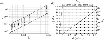
Therefore, with spheres of constant dimensions, the instability will develop at multiple thresholds, not just one, which depends on the magnitude of the electromagnetic forcing and the rotation of the external sphere. Figure 7(a) shows the flow transition map as a function of the dimensionless parameters  $E_k$ and
 $\varLambda _L$, which take into account the rotation effect, whereas figure 7(b) presents the transition map for the experimentally controlled parameters (
 $I$ and
 $\varOmega$) and their associated Reynolds numbers. For a fixed rotation
 $\varOmega =0.314$ (
 $ {\textit {Re}} _o=3460$) and an increasing electromagnetic forcing, the transition elapses from a stable flow (
 $\bullet$) to an anticyclonic rotation of the instability (
 $\square$), and finally to a cyclonic rotation (
 $\odot$). Along these phases, the flow undergoes a transition stage (
 ${_\bigtriangleup}$) in which the instability oscillates between cyclonic and anticyclonic rotation. In general, the stability map does not show a well-established pattern; however, the cyclonic and anticyclonic rotation of the instability are largely present. Additionally, a small oscillation in the flow close to the inner (
 $\blacksquare$) or outer (
 $\blacktriangle$) sphere is also observed, which could be associated with the multiple thresholds that trigger the instability.
Instability map (regime diagram). (a) Dimensionless parameters  $E_k$ and
 $\varLambda _L$. (b) Experimental parameters and their associated Reynolds numbers. Here,
 $\bullet$ indicates stable flow,
 $\odot$ indicates cyclonic rotation,
 ${_\bigtriangleup}$ indicates oscillation,
 $\square$ indicates anticyclonic rotation,
 $\blacksquare$ indicates internal vibration, and
 $\blacktriangle$ indicates external vibration. Numerical simulations.

Even though it is not within the scope of this work to disclose the entire instability mechanism, we analyse it briefly to acquire some insight into its dynamics. First, we examine the case where the flow is driven electromagnetically and the outer sphere is motionless. The basic state consists of a radial jet in the equatorial plane carrying fluid from the inner sphere to the outer sphere (Piedra et al. Reference Piedra, Rojas, Rivera and Figueroa2022). This characteristic is similar to the hydrodynamic SC in the simplest case, where the inner sphere rotates and the outer one is fixed. A meridional circulation that is induced by Ekman pumping at the poles is composed of one or two large vortices in each hemisphere. The flow field is unstable above a critical Reynolds number. The first instability consists of two Taylor vortices straddling the equator, where one of them is larger than the other.
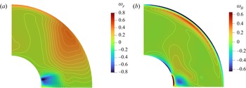
When the outer sphere also rotates, the innermost ring of the Taylor rings is displaced towards the equator, observed in the middle circulation as shown in figure 3. The radial jet interacts with the viscous layer due to the rotation of the outer sphere, and the instability develops in the equatorial region, as seen in figure 8, where the time-averaged radial and azimuthal components of the vorticity are plotted in a meridional plane for the case  $I=50$ mA,
 $\varOmega =0.2531\,{\rm rad}\,{\rm s}^{-1}$. The jet is constrained close to the inner sphere due to the rotation of the external sphere. Another significant difference of the observed jet is that it tends to be wider since it cannot fully propagate throughout the gap. The origin of the instability is in the equatorial region, where high shear is observed and extends in the polar direction as the inclined vortices twist following a helicoidal pattern. It is important to highlight that similarly to the SC case where the instabilities consist of a series of waves on the initially flat radial–azimuthal jet, Hollerbach et al. (Reference Hollerbach, Junk and Egbers2006) found that the azimuthal wavenumber is
 $m=2$, which coincides with the present work since four tornado-like vortices are observed. Finally, because induced effects are negligible, the magnetic field does not attenuate the flow in the regions where it is intense, therefore the instability is purely hydrodynamical even if the flow is electromagnetically driven.
Time-averaged meridional plane of the vorticity: (a)  $r$-component, (b)
 $\theta$-component. Here,
 $E_k=8.12 \times 10^{-4}$ and
 $\varLambda _L=2.15 \times 10^{-2}$ (
 $I=50$ mA,
 $\varOmega =0.251\,{\rm rad}\,{\rm s}^{-1}$). Numerical simulations.

5. Concluding remarks
In this work, we addressed numerically and experimentally the electromagnetically driven flow between two concentric spheres considering the rotation of the outer sphere in the laminar regime. The mainly azimuthal electromagnetic force is generated by the interaction of a direct current injected radially at the equatorial region and a dipolar magnetic field. This flow configuration is a modified version of one of the fundamental problems in fluid dynamics: the rotating spherical Couette flow. However, since electromagnetic stirring is present, the flow now depends on a larger number of parameters, giving rise to a broader set of flow structures. The very small values ( $O(10^{-1})$) of the Hartmann number
 $Ha$ in the present experiment lead to negligible induced effects, while viscous and imposed non-uniform Lorentz forces dominate the flow. Taking advantage of the optical access of the simple experimental set-up, the experimental characterization was performed with PIV in the equatorial plane. Three-dimensional numerical modelling was done using an in-house developed code, and the simulations were compared successfully with the experimental observations. In regions close to the outer sphere, its rotation dictates the motion; however, an anticyclonic flow is well-established close to the inner sphere. Meridional velocity maps show a geostrophic region close to the outer sphere, which agrees with the Proudman–Taylor theorem. Additionally, meridional streamlines exhibit three poloidal vortices, where the innermost vortex is caused by electromagnetic forcing. A hydrodynamic instability is also observed in the equatorial high-shear region. The three-dimensional picture of the instability was reconstructed, showing four helicoidal vortical structures that extend vertically from the equator towards the poles; they are tilted and entangled. The instability map was built for a wide variety of parameters. After analysis and comparison with the hydrodynamic SC flow, it is concluded that the symmetry of the flow is broken due to a shear instability promoted by the interaction between the wide radial–azimuthal jet close to the inner sphere and the azimuthal flow driven by the rotation of the external sphere at the equatorial region. To the best of our knowledge, theoretical and experimental evidence of the instability and the electromagnetically driven anticyclonic flow inside a system of concentrically rotating spheres was found for the first time in this work. Further studies to fully characterize the dynamics of this instability are ongoing work. Even though the investigation addressed in this study of a fundamental nature, we want to highlight the potential use of electromagnetic forcing as an alternative method to induce flows that might be considered relevant in geophysical and astrophysical phenomena.
Supplementary movie
A supplementary movie is available at https://doi.org/10.1017/jfm.2023.183.
Acknowledgements
A.F. and S.P. thank the Investigadoras e Investigadores por México programme from CONACYT. MEng. J. Olvera-Orozco is acknowledged for helping with the grammar and style revision of the manuscript.
Funding
This research was supported by CONACYT, México under project 258623.
Declaration of interests
The authors report no conflict of interest.