

Introduction
Seed germination experiments are conducted in many different biological disciplines. The diverse applications of this powerful tool include studies of physiological processes underlying germination, types and controls of dormancy, plant life histories, determinants of invasiveness in plants, genetic and environmentally induced differences between conspecific populations, seed storage or preparation methods that maximize germination percentage, and post-sowing physical and chemical environmental factors that maximize germination percentage. Baskin and Baskin (Reference Baskin and Baskin2001) provide a wealth of specific examples with references to the literature.
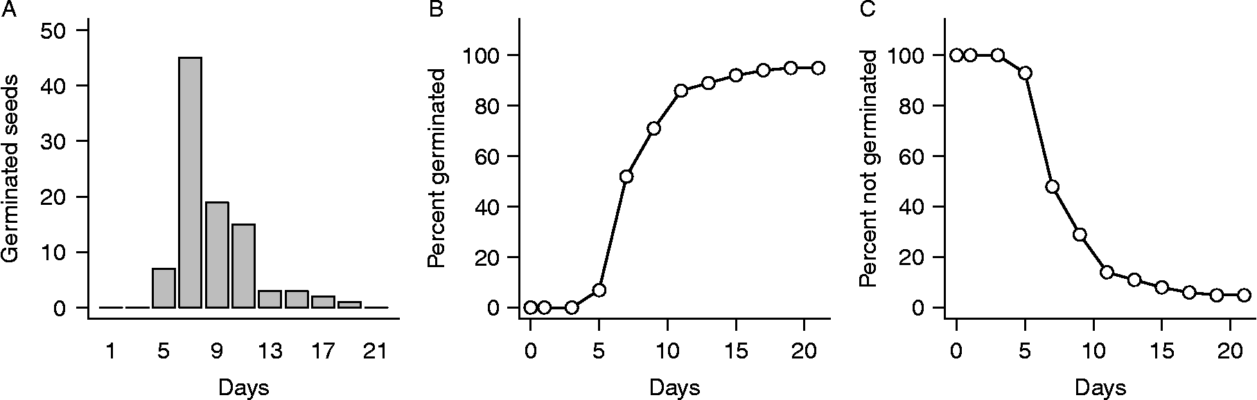
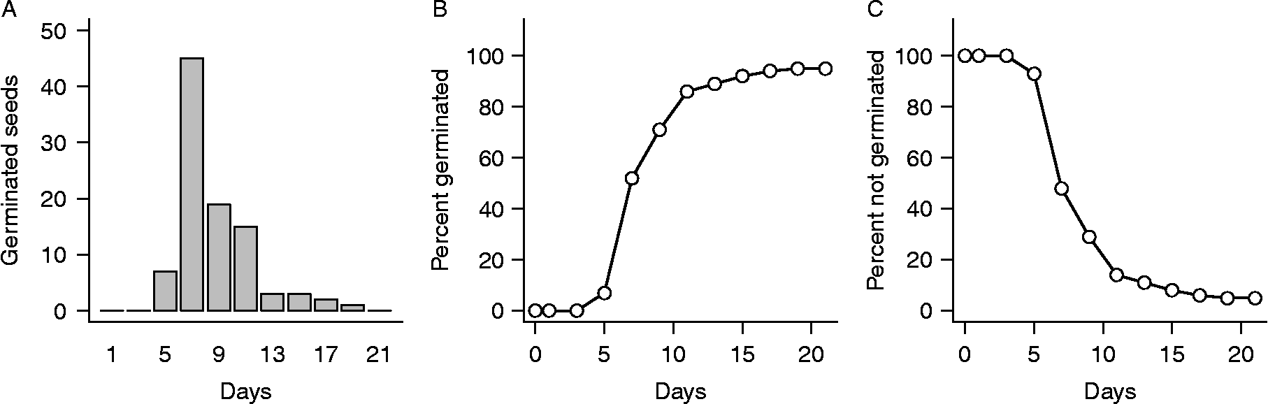
Germination experiments typically are conducted by placing groups of seeds on a moist substrate inside containers (e.g. filter paper or sand in Petri dishes), which are then placed randomly in an incubator under controlled temperature and light conditions. Seeds are checked for germination (operationally defined, usually as radicle emergence) on a sequence of observation days over a fixed period of time, typically chosen to be long enough so nearly all seeds germinate that are capable of doing so under the experimental conditions. On each observation day, seeds found to have germinated since the previous observation are counted and removed, yielding a temporal sequence of germination numbers. An example of such data for Japanese knotweed [Fallopia japonica (Houtt.) Ronse Decraene or Polygonum cuspidatum Sieb. and Zucc.] is shown in Fig. 1.
An example of germination data for seeds of Japanese knotweed. Data are from Bram and McNair (Reference Bram and McNair2004) and are described in the text. (A) Numbers of newly germinated seeds observed on days 1, 3, 5, …, 21 of the experiment. (B) The same data plotted as cumulative totals. This is the form in which data are usually viewed in the germination literature. (C) The same data plotted as percent seeds not yet germinated. This is the form in which data are usually viewed in statistical time-to-event analysis.
To be clear, the term ‘germination’ properly refers to the physiological and developmental processes that resume in mature, non-dormant seeds when they are exposed to appropriate conditions of water availability, temperature and other physicochemical factors. In germination experiments, it is actually the completion of germination that is observed. But to avoid awkward terminology, we will refer to the completion of germination simply as germination in this review. For example, we will refer to the median time at which seeds complete germination as the median germination time, and to the temporal pattern of completion of germination as the temporal pattern of germination. This convenient usage is common in the literature and should cause no confusion here, since we never refer to the actual process of germination.
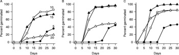
In many applications that employ germination experiments, it is not sufficient merely to determine the percentage of seeds that germinate by the end of the experiment. Nor are data plots such as those shown in Fig. 1 sufficient as a means of communicating results or as a basis for interpreting them. For example, Fig. 2 (based on data from Baskin and Baskin, Reference Baskin and Baskin1983) shows plots of cumulative germination versus time for seeds of Veronica arvensis L. incubated at several different temperatures following storage at 25°C for 2 months (panel A), 3 months (panel B) or 4 months (panel C). Are the curves for 10 and 15°C significantly different in any of the panels? Are the curves for 10 and 20°C significantly different in panel C? Which curves for a given temperature differ significantly between panels? It is simply not possible to answer questions like these by examining this figure, and few meaningful conclusions can therefore be drawn from it. At a minimum, we require rigorous statistical methods for testing hypotheses regarding potential differences in temporal patterns of germination between treatment groups. And methods for testing hypotheses regarding potential effects of quantitative covariates like storage duration and incubation temperature would be highly desirable, as well.
Cumulative germination of Veronica arvensis seeds at four different temperatures (5, 10, 15 and 20°C) after storage for 2 months (A), 3 months (B), or 4 months (C) at 25°C. Data were digitized from Fig. 3 of Baskin and Baskin (Reference Baskin and Baskin1983).

But what statistical methods should be used to test such hypotheses? The problem is complicated by the fact that germination data differ in important ways from types of data usually encountered in biology. For example, data typically are collected by following cohorts of seeds, so the cumulative percentage of seeds that have (or have not) germinated on successive days of observation exhibits serial autocorrelation. Also, ungerminated seeds typically remain when experiments are terminated, and there is no way to be certain when these seeds would have germinated if the experiment had been continued indefinitely. For such seeds, all that is certain is that the time to germination is greater than the duration of the experiment. How, then, can we validly estimate the mean or variance of the germination time? The presence of such right-censored observations violates assumptions of many classical statistical methods, and specialized methods are therefore required.
Numerous methods have been proposed for quantifying different characteristics of temporal patterns of germination like those in Figs 1 and 2. But as several previous authors have pointed out (Goodchild and Walker, Reference Goodchild and Walker1971; Scott et al., Reference Scott, Jones and Williams1984; Brown and Mayer, Reference Brown and Mayer1988a), many of these methods are flawed on conceptual or statistical grounds, or provide information that is inadequate for many applications (see below). An important exception is a relatively new class of statistical methods variously called time-to-event analysis, survival analysis, failure-time analysis and reliability analysis. We will refer to these methods as time-to-event analysis to avoid potentially confusing connotations of the alternative names. These methods are powerful, flexible and statistically sound, but they have only rarely been applied to germination data and are poorly documented in the biological literature.
We believe that the statistical theory and techniques of time-to-event analysis provide the most appropriate and powerful set of methods for analysing germination data. Several previous authors have noted the applicability of these methods (Scott and Jones, Reference Scott and Jones1982; Scott et al., Reference Scott, Jones and Williams1984; Gunjača and Šarčević, Reference Gunjača and Šarčević2000; Fox, Reference Fox, Scheiner and Gurevich2001; Onofri et al., Reference Onofri, Gresta and Tei2010), yet they continue to be underutilized. The main reason seems to be simply that most researchers who conduct germination experiments are not familiar with these methods or their advantages over statistical methods with which they are familiar, such as classical regression analysis and analysis of variance.
The goals of the present paper are to: (1) briefly review and assesses the various commonly used methods of analysing seed germination data; (2) provide a more-detailed review of the main non-parametric and semi-parametric methods of modern time-to-event analysis, including how to apply them specifically to germination data with standard statistical software; and (3) illustrate each method by applying it to real germination data. We restrict our detailed review to methods that are both appropriate for germination data and available in standard statistical software. The main consequence of this restriction is that we provide only a brief overview of fully parametric methods. For reasons we will explain, implementations of these methods currently available in standard statistical software are not appropriate for analysing germination data. But even in medical applications for which these implementations are appropriate, non-parametric and semi-parametric methods are by far the most widely used methods of time-to-event analysis and will suffice for most seed-germination studies.
Review of quantitative methods commonly applied to germination data
Historically, three main approaches have been used for quantitative analysis of seed germination data. The simplest and oldest approach employs intuition-based indexes intended to capture useful information about the temporal pattern of germination. An alternative approach was later developed that uses classical regression techniques to fit non-linear parametric functions to the temporal sequence of cumulative germination. More recently, various types of time-to-event analysis have been applied to germination data. All three of these approaches are currently in use. We briefly review each of them in this section, then review time-to-event methods in more detail in subsequent sections.
Germination indexes
Germination indexes have been reviewed by Scott et al. (Reference Scott, Jones and Williams1984), Brown and Mayer (Reference Brown and Mayer1988a) and Ranal and Santana (Reference Ranal and Santana2006). There is no shortage of such indexes; Ranal and Santana (Reference Ranal and Santana2006) discuss more than 20 of them. Since germination indexes are so numerous and have been thoroughly reviewed, we will content ourselves with a few examples to illustrate the approach.
A very commonly used index is Germinability, which is the cumulative percentage of seeds that have germinated by the end of an experiment. Another common index is Czabator's (Reference Czabator1962) Germination Value, which is the product of the ‘peak value’ and ‘mean daily germination’ for seeds that germinate during an experiment. The peak value is the maximum of the quotients, computed for all observation times, of cumulative germination percentage divided by time since the beginning of the experiment in days. Mean daily germination is the germination percentage at the end of the experiment divided by the duration of the experiment in days. Maguire's (Reference Maguire1962) Speed of Germination is the sum over all observation days of the same quotients used in determining the peak value. Baskin and Baskin (Reference Baskin and Baskin2001) suggest using a modified Timson (Reference Timson1965) index given by the sum of daily cumulative germination percentages observed during a germination experiment. These and other indexes are computed separately for each replicate, and potential differences between groups of seeds (e.g. different sources, different methods of storage or preparation) are assessed via analysis of variance.
Germination indexes are still widely used, but several authors have identified serious conceptual and statistical problems with them (Goodchild and Walker, Reference Goodchild and Walker1971; Scott et al., Reference Scott, Jones and Williams1984; Brown and Mayer, Reference Brown and Mayer1988a). The paper by Brown and Mayer (Reference Brown and Mayer1988a) is especially cogent. The fundamental problem derives from the fact that there are at least four conceptually distinct properties of the temporal pattern of germination that must be quantified in order to fully characterize it: (1) duration of the initial delay in onset of germination; (2) percentage of seeds that ultimately germinate; (3) average speed of germination following onset; and (4) the temporal pattern of change in germination speed following onset (Brown and Mayer, Reference Brown and Mayer1988a; Farmer, Reference Farmer1997). Paraphrasing Brown and Mayer (Reference Brown and Mayer1988a), we may call these properties the delay, extent, average speed and variation in speed of germination. As Brown and Mayer (Reference Brown and Mayer1988a) note, it is simply not possible to characterize all of these properties with a single index, and they will be confounded in any index that includes information about more than one of them. For example, Germinability includes information about only the extent of germination, Germination Value and Germination Speed confound extent and speed, and Timson's index confounds extent, speed and variation in speed (Brown and Mayer, Reference Brown and Mayer1988a).
A potentially serious statistical problem with germination indexes is that they make only limited use of the data from an experiment. An extreme case is Germinability, which utilizes data from only the final observation day, throwing away the rest. Thus, if two sets of germination data exhibit radically different temporal patterns but converge on the last observation day, this index would lead one to conclude that there was no difference between them. This is not a problem in seed technology, since the extent of germination is the main property of interest, and data waste is reduced by employing only two observation days (ISTA, 1985). But in most other applications, differences in temporal patterns of germination are important, as Brown and Mayer (Reference Brown and Mayer1988a) emphasize. Documenting these patterns requires numerous observation days, and most of the resulting data are wasted or poorly used when germination indexes are employed.
For these reasons, and because of their evident subjectivity, we concur with Scott et al. (Reference Scott, Jones and Williams1984) and Brown and Mayer (Reference Brown and Mayer1988a) that germination indexes do not provide an adequate basis for characterizing the temporal pattern of germination, comparing groups of seeds or assessing treatment effects, though Germinability certainly is appropriate for characterizing seed lots in seed technology.
Classical non-linear regression analysis of cumulative germination data
Beginning in the 1970s, an alternative to the use of germination indexes was developed in which generalized curve-fitting programs are used to fit non-linear parametric functions to the temporal sequence of cumulative germination (Goodchild and Walker, Reference Goodchild and Walker1971; Janssen, Reference Janssen1973; Bonner and Dell, Reference Bonner and Dell1976; Tipton, Reference Tipton1984; Brown, Reference Brown1987; Brown and Mayer, Reference Brown and Mayer1988b; Carneiro, Reference Carneiro1994). This approach typically yields estimates of two, three or four function parameters (depending on the specific function fitted), which are then used in place of intuition-based indexes to characterize key features of germination. It has been a common method of analysing germination data since the 1980s and is still widely used. Two examples will illustrate the key features of the approach.
Tipton (Reference Tipton1984) fitted three classical three-parameter growth functions (monomolecular, logistic and Gompertz; for definitions, see Draper and Smith, Reference Draper and Smith1998) to cumulative germination data for creosote bush (Larrea tridentata). Each function included a shape parameter, a temporal scale parameter and a germinability parameter. For example, the Gompertz growth function has the following form:

where F(t) is the proportion of seeds that have germinated by time t, p is the germinability parameter (proportion of seeds capable of germinating under the experimental conditions), λ is the temporal scale parameter, and α is the shape parameter. None of the functions included an initial delay in onset of germination. Brown (Reference Brown1987) fitted the following four-parameter Weibull cumulative distribution function to cumulative germination data for Aristida armata seeds:

where F(t), p, λ, and α are defined as in equation (1), τ is a delay parameter representing the initial delay in onset of germination, and we define F(t) = 0 for t < τ. The four parameters in this model characterize all four key properties of the temporal pattern of germination.
Researchers using this approach typically fit their growth or cumulative distribution functions to temporal sequences of observed cumulative germination using general-purpose non-linear regression software. Since parameters in the most commonly used growth or cumulative distribution models have reasonably clear biological meanings, they are often used in a manner similar to germination indexes. For example, parameters are commonly estimated separately for each of several replicates, and potential differences between treatment groups are assessed via analysis of variance.
A limitation of the classical non-linear regression approach is that cumulative germination data violate a basic requirement of standard non-linear regression models. Because seed germination experiments involve repeated observations on the same cohort of seeds, the cumulative number of seeds that have germinated by day t+1 is not independent of the number that have germinated by day t, resulting in positive autocorrelation of the residuals (deviations between observed and expected values) at successive values of t. But the statistical theory used to construct confidence intervals and test hypotheses in standard non-linear regression programs requires the residuals to be uncorrelated. Therefore, while these programs may be used to estimate model parameters (which is the usual practice, outlined above), all the other information these programs provide that normally would be of great importance – confidence intervals for parameters and the fitted function, hypothesis tests for parameter values, and comparisons of parameter values for fitted functions for two or more groups – must be disregarded. This problem reflects the fact that the regression program is being applied to data for which the underlying statistical model is inappropriate. Time-to-event analysis resolves this problem by focusing on the fates of individual seeds rather than cumulative germination.
Time-to-event analysis
As noted in the Introduction, there are three major types of time-to-event analysis: non-parametric, semi-parametric and fully parametric. Non-parametric time-to-event analysis comes in two main flavours: a traditional approach based on actuarial life-table methods and a more recent approach based on modern statistical theory. The semi-parametric approach consists of the Cox proportional hazards model and various extensions. The fully parametric approach includes so-called accelerated life (or accelerated failure-time) models, as well as many other parametric models. All three major types of time-to-event analysis are based on the distribution of germination times of individual seeds rather than on cumulative germination.
A few papers in the literature have applied non-parametric time-to-event analysis to germination data (Scott and Jones, Reference Scott and Jones1982; Scott et al., Reference Scott, Jones and Williams1984; Gunjača and Šarčević, Reference Gunjača and Šarčević2000). All of these employ only classical life-table methods, which were designed for use with census data and are rarely used in modern time-to-event analysis. More recent and more diverse methods designed for data where exact event times are assumed to be known have several theoretical advantages over life-table methods, and for this reason are now by far the most commonly applied non-parametric methods in medical applications of time-to-event analysis. To our knowledge, no review of these modern non-parametric methods as applied to germination data is currently available.
Scott et al. (Reference Scott, Jones and Williams1984) apply semi-parametric time-to-event analysis (Cox proportional hazards model) to germination data, while Fox (Reference Fox, Scheiner and Gurevich2001) briefly discusses the method but does not apply it. The descriptions provided by Scott et al. (Reference Scott, Jones and Williams1984) and Fox (Reference Fox, Scheiner and Gurevich2001) include some of the basic ideas behind the proportional hazards model but are too brief to be useful guides for applying them.
Fully parametric time-to-event analysis is the most natural and statistically sound way to implement the type of detailed analysis that previous investigators have attempted by fitting non-linear regression models to cumulative germination data. However, to our knowledge, all previous papers addressing applications of time-to-event analysis to germination data either do not discuss the fully parametric approach or else discuss special cases that, on close examination, turn out to be inappropriate for application to germination data. For example, Scott et al. (Reference Scott, Jones and Williams1984) and Onofri et al. (Reference Onofri, Gresta and Tei2010) apply the accelerated life model to data on time to germination, and Fox (Reference Fox1990, Reference Fox, Scheiner and Gurevich2001) applies the same model to data on time to seedling emergence, but the form of the model these authors discuss (which is the only form currently available in standard statistical software) actually is not appropriate for seed germination or seedling emergence data. The reason is that the standard version of the accelerated life model cannot accommodate either delays in the onset of germination or mixtures of germinable and non-germinable seeds, whereas germination data typically exhibit both of these properties.
Terminology, test data and statistical software
Before beginning our review of non-parametric and semi-parametric methods, we introduce some basic concepts and terminology that will be required. We also describe test data and statistical software that will be used to illustrate application of these methods to germination data.
Basic probability functions
Non-parametric and semi-parametric methods of time-to-event analysis are based mainly on two probability functions: the survivor function (or complementary cumulative distribution function) and the hazard function. Understanding the statistical methods requires a basic understanding of these functions, which we therefore briefly review.
The time required for a seed to germinate, or germination time, is a random variable. The associated survivor function S(t) is the probability that the germination time is greater than t. We assume the germination time is always greater than 0, so S(0) = 1. As t increases from 0, S(t) typically will remain constant at a value of 1 for small values of t (due to the initial delay in onset of germination) and then begin to decrease. As t becomes large, S(t) will approach a limiting value which is either 0 (if all seeds are capable of germinating under the experimental conditions) or somewhat greater than 0 (otherwise).
The hazard function h(t) is defined such that h(t)dt is the probability that the germination time lies in the infinitesimal interval (t, t+dt], given that it is greater than t. We have

where f(t) = − dS/dt is the probability density function, defined such that f(t)dt is the probability that the germination time lies in the infinitesimal interval (t, t+dt]. The hazard function tells us how likely it is that a seed which has not germinated by time t will germinate shortly after t. It has dimensions of 1/time and is often called the hazard rate.
The following relationship between the survivor function and the hazard function is important and will be used below:

Thus, increasing the hazard rate will decease the survivor function.
Observation schemes and data types
An observation scheme is a temporal pattern of seed monitoring. A variety of observation schemes are employed in different applications of time-to-event analysis (see Lawless, Reference Lawless2003), but two types are important to know about when analysing germination data. We call these periodic simultaneous observation and continuous observation, and we call the corresponding types of data interval data and exact data.
Periodic simultaneous observation and interval data
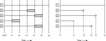
The observation scheme employed in standard germination experiments is illustrated in the left panel of Fig. 3 and can be described as follows. All seeds are placed in an incubator at the same time and are then observed at predetermined times 0 = a 0 < a 1 < a 2 < a 3 < … < a m < ∞. At each observation time a i, all seeds are examined, and those whose radicles are protruding are recorded as having germinated in the interval (a i − 1, a i] and are discarded. Care is taken to ensure that the amount of time required to check all seeds is negligible compared to the length of time a i − a i − 1 between successive observation times. If any seeds are lost or damaged between observations a i − 1 and a i, the number is recorded and assigned to interval (a i − 1, a i]. The number of ungerminated seeds remaining at the (predetermined) final observation time a m is also recorded. Germination times of these seeds are only known to exceed a m and so are right-censored.
Two types of observation scheme assumed in standard methods of time-to-event analysis. Both panels show the fates of five seeds during a germination experiment. A germination event is indicated by a circle, a censoring time by an ‘x’. The final censoring time (seed 1) occurs at the end of the experiment, indicating that the seed had not yet germinated. The other censoring time (seed 4) occurs during the experiment, indicating seed loss. In the left panel, observations are made only at planned times a i. When a germinated seed is observed at time a i, all that is known is that the germination event (grey circle) occurred sometime during the interval between observation times a i − 1 and a i (enclosed by a rectangle). Similarly, when a seed is found to be missing at observation time a i, all that is known is that the loss (grey ‘x’) occurred sometime between times a i − 1 and a i. This is the observation scheme for which life-table methods of time-to-event analysis were originally designed. In the right panel, all censoring times and uncensored germination times t i* are assumed to be known exactly, while censored germination times are only known to exceed the censoring time. This is the observation scheme assumed by the Kaplan–Meier estimator of the survivor function and by most other modern methods of time-to-event analysis.

We call this observation scheme ‘periodic simultaneous observation’ because seeds are observed periodically rather than continuously, and because all observations are, to a good approximation, simultaneous. We call the data that are produced ‘interval data’ because they represent the numbers of germination events (and sometimes, seed losses) occurring within the various time intervals.
Continuous observation and exact data
The continuous observation scheme is illustrated in the right panel of Fig. 3 and can be described as follows. As with periodic simultaneous observation, the germination experiment begins by placing all seeds in an incubator at the same time. Now, however, we assume that every seed is continuously monitored. If any seeds are lost during the experiment, we assume the exact loss times are known. For lost seeds, all we know regarding germination is that the germination time is greater than the loss time, so the germination time is right-censored. Of the seeds not lost, some might not germinate by the (predetermined) end of the experiment, so the time to germination will be right-censored for these seeds, as well. All the remaining seeds will germinate during the experiment, and we assume their germination times are known exactly.
For obvious reasons, we call this observation scheme ‘continuous observation’. And since the data for seeds that germinate during the experiment represent exact germination times, we call them ‘exact data’.
While data generated by standard germination experiments clearly are of the interval type, it is sometimes necessary or desirable to analyse them using statistical methods designed for exact data. The main reason is that most of the methods available in current statistical software assume exact data. But as we will explain below in our review, it is almost always safe and appropriate to apply methods designed for exact data to germination data.
Test data
We will illustrate all the main methods of non-parametric and semi-parametric time-to-event analysis by applying them to germination data for Japanese knotweed seeds. These data come from a study by Bram and McNair (Reference Bram and McNair2004), whose main purpose was to assess the potential for sexual reproduction by invasive Japanese knotweed populations growing along streams in south-eastern Pennsylvania, USA. Methods of seed collection, preparation and germination testing are described in detail by Bram and McNair (Reference Bram and McNair2004) but, for completeness, we provide a brief overview here.
Seeds from invasive Japanese knotweed populations were collected weekly from three riparian study sites (Carroll Park, Friends Hospital and Rising Sun) in urban forests of Philadelphia, Pennsylvania, USA from 11 September through 1 November 2000 (collection dates 1–8). Seeds were air-dried, then stratified in moist, sterile sand in a cold room at approximately 4°C for 30 d. Following stratification, 100 seeds from each site–date combination were planted in plug flats containing standard potting soil. One seed was planted in each well, just beneath the soil surface. Flats were placed in a growth chamber with alternating periods of light and dark, and high and low temperatures, simulating conditions in the field. Flats were surface-watered and monitored for germination (operationally defined as cotyledon emergence) on day 1, then every 2 d until day 21. The duration of the experiment was chosen based on pilot experiments, in which the cumulative number of germinated seeds from all collection dates and sites appeared to approach a plateau by day 21.
Statistical software
Each method of time-to-event analysis discussed below in our review will be illustrated using R or SAS software. In most, but not all, cases, both programs provide the required functionality with built-in functions or procedures specifically designed for time-to-event analysis. The examples were computed using R version 2.10.1 under the OpenSUSE 11.1 Linux operating system (R Development Core Team, 2009) and SAS version 9.1.3 under the Windows XP operating system (SAS Institute Inc., 2004). Most other widely used statistical programs have modules for time-to-event analysis that provide similar functionality.
Non-parametric time-to-event analysis of germination data
Two main problems can be addressed with non-parametric methods: characterizing the temporal pattern of germination within individual groups of seeds, and comparing patterns of germination in different groups. For each problem, two main classes of methods are available, according as the data are assumed to be of interval or exact type.
Characterizing the temporal pattern of germination
Non-parametric methods of time-to-event analysis allow one to obtain quantitative estimates of the survivor function without assuming a particular functional form. Information that can be obtained with standard statistical software includes, for example, the estimated survivor function and point-wise confidence intervals.
Interval data
Long before the emergence of time-to-event analysis as a statistical discipline in its own right, methods for estimating the survivor function for human populations were developed by actuaries as part of the procedure for constructing life tables. These methods employed census data and therefore assumed periodic simultaneous observation and interval data. Because of its origin, the most commonly used method of this type for estimating the survivor function is usually called the life-table or actuarial estimator, which we now describe.
The observation scheme for interval data is illustrated in the left panel of Fig. 3. Let the initial number of seeds be N. Given observation times 0 = a 0 < a 1 < a 2 < … < a m < ∞, let the intervals between observations be I j = (a j − 1, a j] for j = 1, 2, 3, …, m. We assume the I j are long enough relative to the rate at which germination events occur so that multiple events commonly occur within an interval. Let D j be the number of germination events occurring within interval I j. We assume D j is known but the exact event times are not. Finally, let N i be the number of seeds at risk of germination (i.e. not yet germinated or lost) at the beginning of interval I i, with N 1 = N.
If no seeds are lost before the end of the experiment, then the standard life-table estimator  of the survivor function at the observation times a i is given by

On the other hand, if seed losses do occur before the end of the experiment, it is necessary to adjust the N i to account for the fact that because lost seeds cannot contribute to the observed number of germination events during an interval, they effectively reduce the number of seeds at risk below N i. Letting N i′ denote the adjusted or effective number of seeds at risk, the resulting estimator of the survivor function is

where it remains to specify N i′. The traditional choice of N i′, and the one implemented in standard statistical software, is

where W i is the number of losses during interval I i. Derivations of the above formulas are straightforward and can be found in, for example, Elandt-Johnson and Johnson (Reference Elandt-Johnson and Johnson1980), Lawless (Reference Lawless2003), and Lee and Wang (Reference Lee and Wang2003).
Equations (5), (6) and (7) tell us how to estimate the survivor function at the observation times, but how do we estimate its value at intermediate times? Recalling that the observation times are chosen in such a way that multiple events will occur in many of the intervals between observations, it is most reasonable to assume events occur more or less uniformly during each interval I i and therefore to estimate S(t) for a i < t < a i+1 simply by linearly interpolating between  and
 . This is the result obtained by plotting the estimated survivor function
 versus observation times a i and choosing the graphics option to connect each pair of successive points with a straight line.
Methods are available in standard statistical software for estimating various other functions of interest, including the probability density function, hazard function and corresponding point-wise 95% confidence limits. Neither R nor SAS currently reports the median or other quantiles for the life-table estimate of the survivor function, but the required methods are straightforward (see Lee and Wang, Reference Lee and Wang2003).
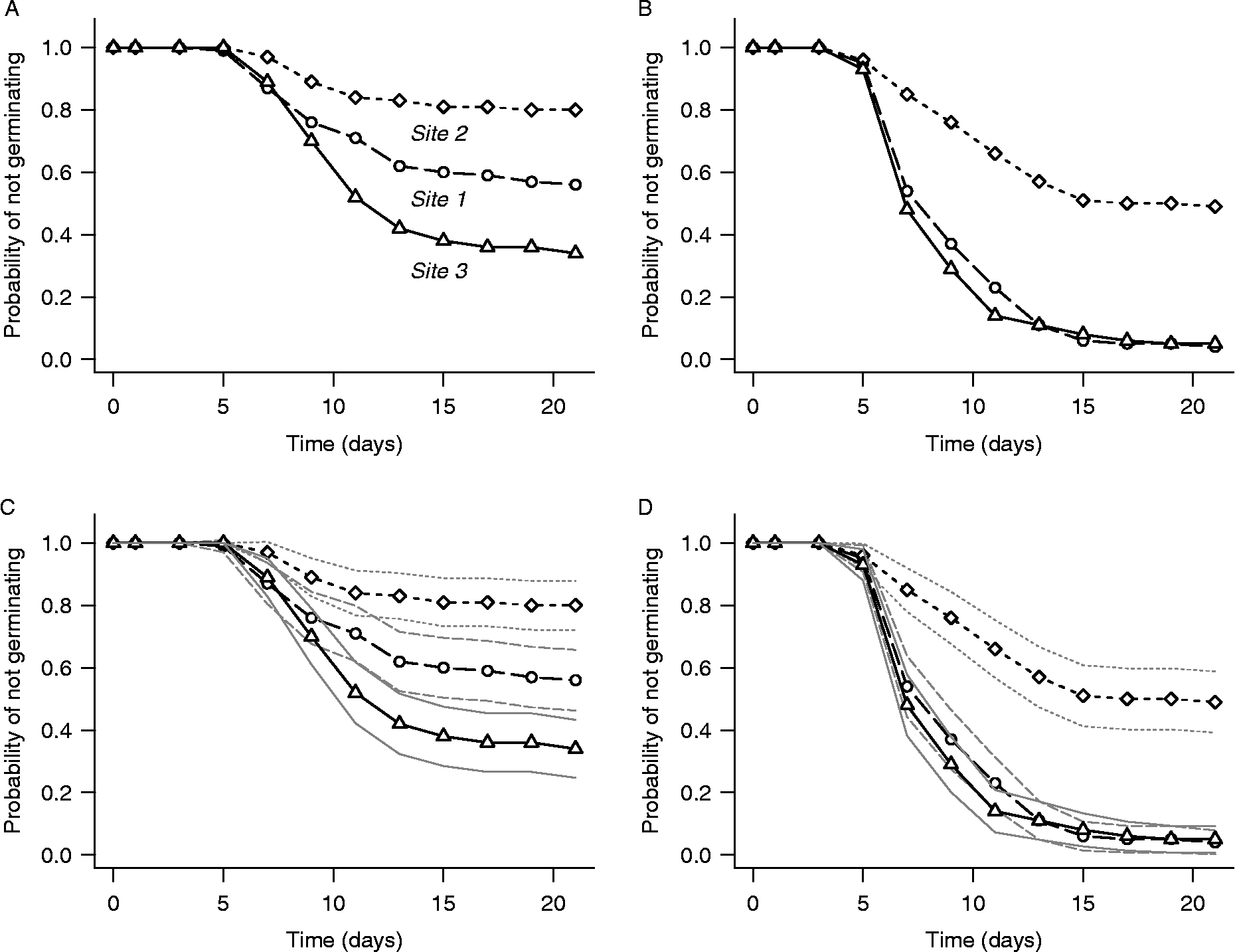
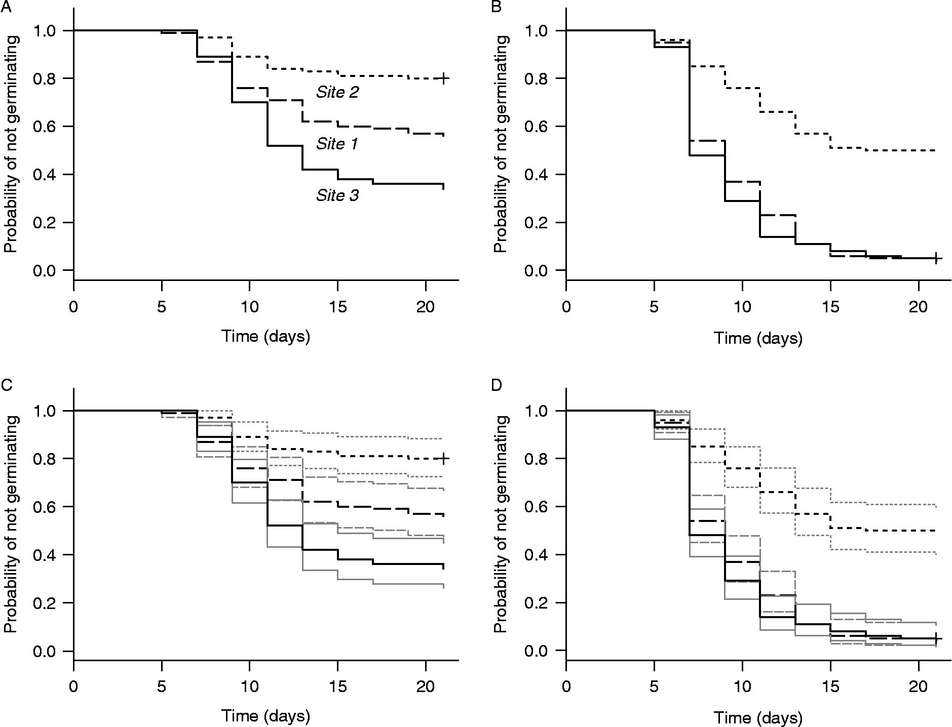
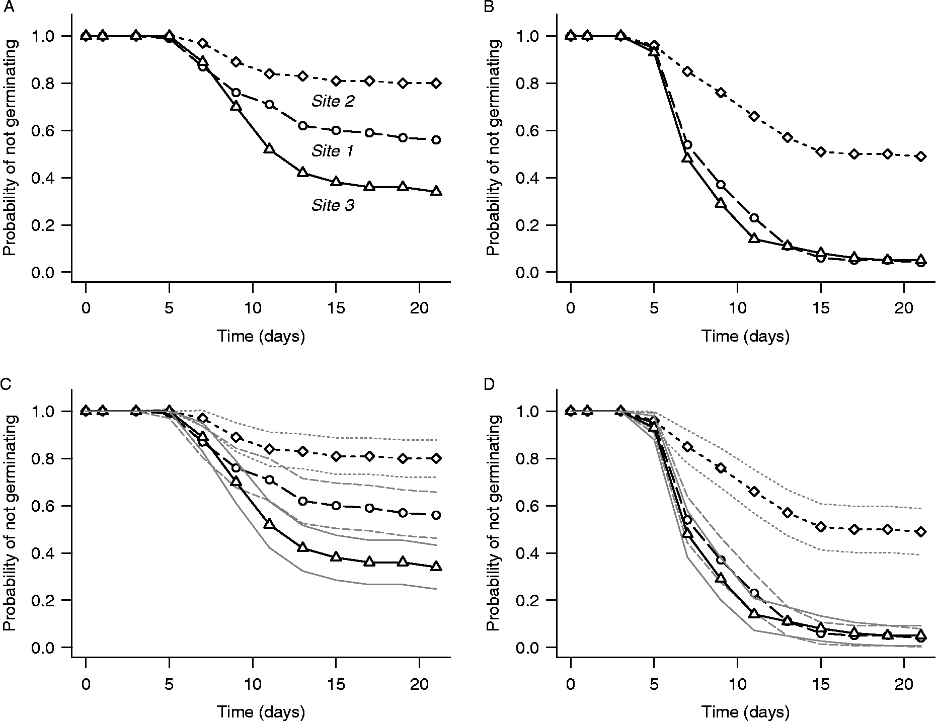
Figure 4 shows life-table estimates of survivor functions computed for the three study sites in the test data using R function lifetab() from the KMsurv package. Examples are plotted for collection dates 3 and 8, without (panels A and B) and with (panels C and D) point-wise 95% confidence intervals. lifetab() creates an object whose components include estimates and point-wise standard errors of the survivor function, probability density function and hazard function. Plots like those of Fig. 4 must be created from this object using the default R plot function. Various types of point-wise 95% confidence intervals can be constructed using the Greenwood standard errors created by lifetab(). Those in Fig. 4 assume a normal distribution of  :
 , where SEi is the standard error of
 .
Life-table estimates of survivor functions for Japanese knotweed seeds collected from three study sites on collection dates 3 (left panels) and 8 (right panels), computed by R function lifetab() from the KMSurv package. The lower panels are the same as the upper panels, except that point-wise 95% confidence intervals (thin lines) have been added. Confidence intervals are based on a normal approximation using Greenwood standard errors computed by lifetab(); see text for details.
The SAS procedure lifetest also allows one to estimate life-table survivor functions, but it is important to note that it does so incorrectly for interval data generated by periodic simultaneous observation unless the data or observation times are adjusted so that the values entered as event times are slightly less than the observation times (see the online supplementary material, available at http://journals.cambridge.org/).
Sample R and SAS code for estimating the survivor function using methods for interval data is provided in the supplementary material.
Exact data
Estimates of the survivor function when event times are assumed to be exact (but with ties permitted) are usually obtained with the Kaplan–Meier estimator. The origin of this estimator can be traced back to the product-limit estimator of Böhmer (Reference Böhmer1912) in the actuarial literature. It is sometimes called the product-limit estimator in the statistical literature, but Kaplan and Meier (Reference Kaplan and Meier1958) provided the first derivation based on modern statistical concepts.
The Kaplan–Meier estimator of the survivor function is designed for exact data produced by a continuous monitoring scheme, as illustrated in the right panel of Fig. 3. Let t 1*, t 2*, t 3*, …, t N* denote the times at which the N initial seeds either germinate or are censored (including censoring by termination of the experiment and seed loss), and let δ1, δ2, δ3, …, δN be status variables that tell us whether the corresponding t i* values are germination times (δi = 1) or censoring times (δi = 0). (Note: in data files used for analysing data that are treated as exact, every seed is represented by its pair of t i* and δi values.) We allow the possibility that some of the t i* are identical, in which case the data contain ties. Let t 1 < t 2 < t 3 < … < t k (k ≤ N) be the distinct times at which germination events occur, and let d j be the number of germination events that occur at t j. Finally, let n i be the number of seeds that were at risk of germination immediately prior to t i. Then the Kaplan–Meier estimator  of the survivor function is given by

where i is the index of the observed germination times. (For derivations, see Cox and Oakes, Reference Cox and Oakes1984; Lawless, Reference Lawless2003.) Note that  is a step function that changes (decreases) only at values of t at which germination events occur, and that the effect of seed loss is to reduce n j.
How do the Kaplan–Meier and life-table estimates of the survivor function compare when they are applied to the same germination data? For standard germination experiments, the data will be of interval rather than exact type, so we apply the Kaplan–Meier estimator by treating the actual observation times a i as if they were infinitesimally greater than the unknown germination times t i for intervals in which germination events occurred. We also treat the known number D i of germination events in interval I i as if it were the number d i of (tied) events occurring at distinct event time t i, and we treat the known number N i of seeds at risk at the beginning of interval I i as the number n i at risk immediately prior to event time t i. At the actual observation times, then, the Kaplan–Meier estimator is

Comparing equation (9) with equation (8), we see that the values of the Kaplan–Meier and life-table survivor functions will be identical at the observation times when there are no seed losses. When seed losses occur, the two estimators will differ (because they account for losses differently), but numerical examples suggest that they will be very similar at the observation times if the proportion of seeds lost is less than roughly 5%. This is not much of a restriction, since 5% seed loss would normally be considered unacceptable for other reasons and the experiment would be repeated.
Standard statistical software also provides methods for estimating various other quantities and functions associated with the distribution of germination time, such as the median, probability density function and hazard functions, plus corresponding confidence intervals. Since the Kaplan–Meier estimator produces a step function, there typically will not be an estimated value that exactly corresponds to the median (or other quantile). The usual estimate of the median is the smallest event time t i such that  .
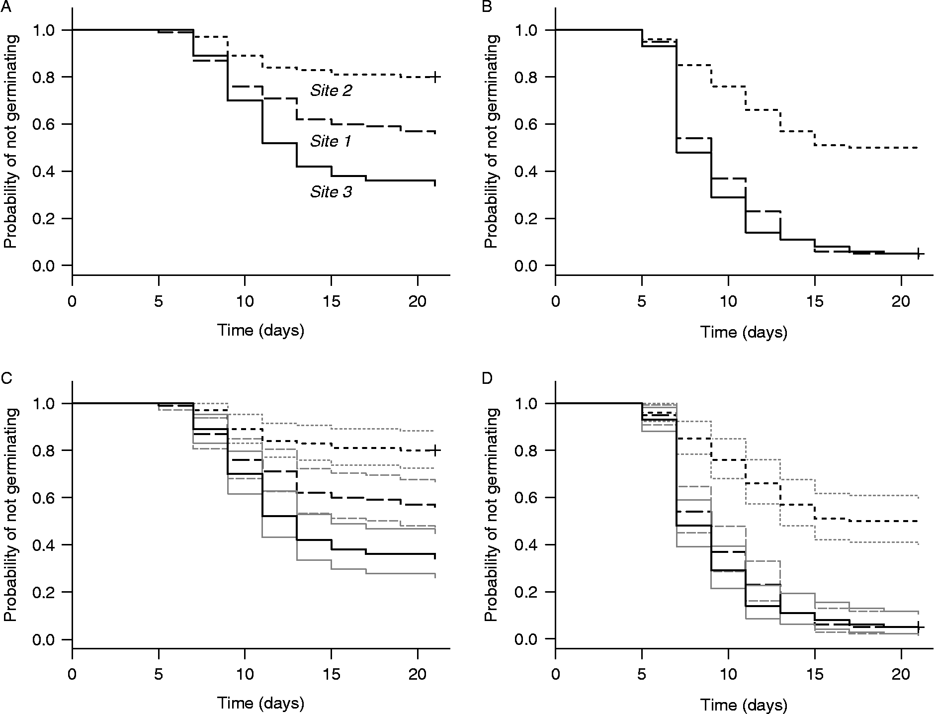
Figure 5 shows Kaplan–Meier survivor functions computed for the three study sites in the test data using R function survfit() from the survival package. These functions are shown for collection dates 3 and 8 without (panels A and B) and with (panels C and D) point-wise 95% confidence intervals. The survfit() function also creates tabular output that is stored in an object whose fields include estimates of the median and 95% confidence limits of the time to germination, as well as the survivor function and its point-wise standard errors and 95% confidence limits. SAS procedure lifetest also can be used to plot Kaplan–Meier survivor functions and to create corresponding tabular output.
Kaplan–Meier estimates of survivor functions for the same data as in Fig. 4, computed by R function survfit() from the survival package. The lower panels are the same as the upper panels, except that point-wise 95% confidence intervals (thin lines) computed by survfit() have been added.
Sample R and SAS code for estimating the survivor function using methods for exact data is provided in the online supplementary material.
Comparing groups
The estimated survivor functions with point-wise confidence intervals in Figs 4 and 5 suggest that the temporal pattern of germination is different for all three study sites for seeds collected on date 3. For seeds collected on date 8, however, the figures suggest that the pattern is the same for sites 1 and 3 but different for site 2. Time-to-event analysis provides several non-parametric techniques for rigorously testing such hypotheses regarding potential group differences in the temporal pattern of germination. One can test for homogeneity of a set of three or more groups, or conduct pairwise tests to determine whether specific pairs of groups are statistically significantly different, all without assuming a parametric form for the survivor function.
Interval data
At the time of this writing, neither R nor SAS provides interval-data methods for comparing life-table survivor functions. For this reason, we relegate discussion of these methods to the supplementary material. We note, however, that both R and SAS include an exact-data version of the Mantel–Haenszel test (the main interval-data test; see the supplementary material) that is usually called the log-rank test. When applied to standard germination data, the log-rank test will give the same results as the Mantel–Haenszel test if there are no seed losses. When a small proportion of seeds are randomly lost, the values of the test statistics usually will remain very similar. Therefore, provided seed loss is absent or rare (e.g. roughly 5% or less), the R or SAS log-rank test can be used for comparing groups in germination experiments, even though the data are of interval rather than exact type.
Several other common methods for comparing groups with exact data are straightforward extensions of the log-rank test. Because of their fundamental similarity to the log-rank test, we argue that it is also appropriate to analyse germination data using these other exact-data tests, which we describe next.
Exact data
A good discussion of methods for comparing groups when the data are assumed to be exact is provided by Klein and Moeschberger (Reference Klein and Moeschberger2003). To keep our review reasonably non-technical, we confine our presentation to a brief summary of the basic ideas behind these tests and a brief discussion of specific tests available in R and SAS.
Suppose there are K ≥ 2 groups, and let t 1 < t 2 < t 3 < … < t D be the distinct event times when data from all groups are combined. Let O ij be the observed number of germination events at time t i in group j, and let E ij be the corresponding expected number of germination events under the null hypothesis that the groups do not differ at any of the event times. The most commonly used non-parametric tests for comparing groups in time-to-event analysis are based on statistics Z j(t′) given by

where j = 1, 2, 3, …, K are the K groups being compared, t′ is the largest time at which there is at least one seed at risk in every group, and w(t i) is a weight function that can be chosen to place equal, increasing or decreasing emphasis on successive event times. The actual test statistic Q that is used to assess the null hypothesis is a quadratic form constructed from any K − 1 of the Z j(t′) (the full set sums to zero, so only K − 1 of them are independent). Two facts about Q are important. First, Q increases as the weighted differences w(t i)(O ij − E ij) between observed and expected numbers of germination events increase. And second, the distribution of Q in large samples is approximately chi-squared with K − 1 degrees of freedom, so the null hypothesis will be rejected if Q is sufficiently large (for additional details, see Klein and Moeschberger, Reference Klein and Moeschberger2003).
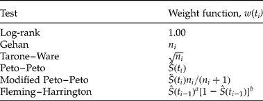
The various tests based on quadratic form Q differ only in the choice of weight function w(t′i). The most common tests and associated weight functions are listed in Table 1. Note that the log-rank test weights all event times equally, while all other tests except Fleming–Harrington place heavier weight on early event times (for which there are the most data) than on late event times. The Fleming–Harrington test is very flexible and is the only test capable of weighting late event times more heavily than early event times. It is convenient to refer to all these tests as generalized log-rank tests. They are best viewed as tests for differences in hazard rate, since the number of seeds at risk in each group at each event time is regarded as fixed.
Common non-parametric tests for determining whether two or more survival functions are statistically significantly different (modified from Table 7.3 of Klein and Moeschberger, Reference Klein and Moeschberger2003). The associated weight function is shown for each test. Notation: n i is the total number of seeds at risk immediately prior to distinct event time t i,  is Kaplan–Meier estimator (equation 8) of the text,
 is the same except that product terms 1−d i/n i are replaced by 1−d i/(n i +1) where d i is the total number of observed germination events at t i, and a and b are non-negative parameters

Methods for comparing the survival patterns for two or more groups with data assumed to be exact (but with ties allowed) are available in both R (function survdiff() in package survival) and SAS (procedure lifetest), and sample code for both software programs is provided in the supplementary material. At the time of this writing, R function survdiff() provides only the Fleming–Harrington test with b = 0, which specializes to the log-rank test when a = 0 and is similar (but not identical) to the Peto–Peto test when a = 1. (Parameters a and b are defined in Table 1.) SAS procedure lifetest currently provides all the tests listed in Table 1.
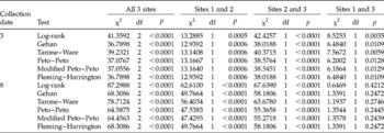
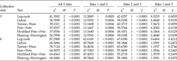
Table 2 shows examples of results computed with SAS procedure lifetest for collection dates 3 and 8 in the test data. For each collection date, results are shown for tests of homogeneity of the three sites, followed by results of the three possible pair-wise tests. Note that, as suggested by Fig. 5, and regardless of which test is employed, the three sites are statistically significantly different from each other on collection date 3, whereas sites 1 and 3 differ from site 2 but not from each other on collection date 8.
Results of group (site) comparisons for seeds collected on dates 3 and 8, illustrating the six tests listed in Table 1. Tests were performed with SAS procedure lifetest using the default parameter values for the Fleming–Harrington test (a=b=1). The three p values for each pairwise test are Holm-adjusted for multiple comparisons
The issue of replicates
It will be noted that we did not mention experimental replicates in connection with any of the non-parametric methods discussed above. The reason is that replication is not necessary for rigorous time-to-event analysis and, indeed, is almost never used in medical applications. If replicates are employed, the data normally would be combined within treatments when using non-parametric methods of time-to-event analysis. An extension to semi-parametric and fully parametric methods allows one to assess random variation among replicates using so-called frailty models (discussed below), but these models are parametric and thus incompatible with non-parametric methods.
Semi-parametric time-to-event analysis of germination data
The main benefit of semi-parametric methods of time-to-event analysis is that they allow one to assess potential effects of multiple covariates, including both categorical and quantitative covariates, while still not requiring one to assume a fully parametric form for the survivor function. In medical applications of time-to-event analysis, the semi-parametric Cox model ‘has become by a wide margin the most used procedure for modeling the relationship of covariates to a survival or other censored outcome’ (Therneau and Grambsch, Reference Therneau and Grambsch2000, p. 39), and it is the only semi-parametric approach that is well supported by standard statistical software. For these reasons, the Cox model is the only semi-parametric method we will discuss.
The Cox model is robust, flexible, extensible and reasonably powerful; it can accommodate categorical and quantitative covariates with fixed effects, it can accommodate random effects and it requires few parametric assumptions. We therefore think it has great potential as a tool for statistical analysis of germination data. We treat this method at greater length than the others, because applying the Cox model requires more steps, and the manner in which results of the analysis are interpreted will be unfamiliar to most biologists.
The Cox proportional hazards model
The Cox model is based on the hazard function rather than the survivor function. The basic idea behind the model is that the hazard function h(t|x) at time t, given a vector x = [x i] of covariates, can be expressed as the product of a baseline hazard function that depends only on time, and a modifier function that depends only on the covariates. That is,

where h 0(t) is the baseline hazard function (whose form need not be specified; see below), x i is the i-th covariate, βi is the slope coefficient for the i-th covariate, β and x are the vectors [βi] and [x i], and ψ is a function that typically is taken to be the exponential function, as in equation (11). An important advantage of the Cox model over non-parametric methods is that it permits quantitative covariates. Categorical covariates are also permitted, and these are coded using indicator (or ‘dummy’) variables, as in ordinary least-squares regression.
The βi coefficients in equation (11) capture information about the relationship between the corresponding covariates and the hazard function. One can see that this model has a feel similar to an ordinary regression model. It is called semi-parametric because no parametric assumptions are made about the baseline hazard function, while the covariate portion does depend on parameters. In this most basic form of the Cox model, it is assumed that none of the βi or x i depends on time, though this assumption can be relaxed in extensions of the model (see Cox and Oakes, Reference Cox and Oakes1984; Therneau and Grambsch, Reference Therneau and Grambsch2000; Klein and Moeschberger, Reference Klein and Moeschberger2003; Lawless, Reference Lawless2003).
Just as in ordinary regression, the goal is to estimate the βi and then test to see if they are significantly different from 0. Estimation of the βi is done through a process called partial likelihood, which is similar to the more traditional likelihood approaches seen in other contexts. In its pure form, this process assumes strict continuous observation and exact data and therefore does not accommodate tied event times. However, even in medical applications for which the Cox model was originally developed, tied event times are very common, and modifications of partial likelihood estimation have therefore been developed to accommodate them. Standard statistical software typically includes at least two such modifications: the Breslow method and the Efron method (see Therneau and Grambsch, Reference Therneau and Grambsch2000). For germination data, where ties are created by the observation scheme, we recommend the Efron method, which provides a good combination of accuracy and computational speed.
A highly desirable feature of the Cox model is that the βi have an easily understood interpretation. They are related to what is commonly called the hazard ratio. To understand the interpretation, consider a categorical covariate x 1 with two levels, coded as 1 and 0. Suppose we have an estimate of the corresponding slope coefficient β1, denoted by  . Then the hazard ratio (HR) for one group relative to the other is

Suppose that  . This means that the hazard function for the first group is twice as large as that for the second group. Therefore, a seed that has not germinated by time t is twice as likely to germinate in the next short interval of time if it comes from group 1 than if it comes from group 2.
Note that the baseline hazard function cancels from the hazard ratio in equation (12). The hazard ratio therefore is constant with respect to time, which is why the Cox model is called the proportional hazards model. This is an important assumption of the Cox model and should be checked. There are a variety of ways to do so, including graphical methods as well as formal tests (e.g. see Andersen et al., Reference Andersen, Borgan, Gill and Keiding1993; Therneau and Grambsch, Reference Therneau and Grambsch2000; Klein and Moeschberger, Reference Klein and Moeschberger2003; Lawless, Reference Lawless2003). We prefer graphical methods for several reasons. Most importantly, because the proportional hazards (PH) assumption will always be a simple approximation to a pattern that is more complex in reality, it is virtually certain that this assumption will be rejected by a formal test if the sample size is sufficiently large, even if it provides a reasonable approximation (as Klein and Moeschberger, Reference Klein and Moeschberger2003, point out). On the other hand, a formal test can easily accept the PH assumption if the sample size is small, even if it provides a poor approximation, since the null hypothesis is that the assumption is met.
A common graphical method of testing the PH assumption, available in both R and SAS, is to plot  versus t or log(t) for different values of covariate vector x (restricted to values of t such that 0 < S(t) < 1), where S(t) is a life-table or Kaplan–Meier survivor function. Under the PH assumption, different covariate values will produce functions with the same shape but different elevations (see the supplementary material). The Cox model is reasonably robust, so it is only necessary to worry about clear departures from proportionality, as indicated by decisive crossing of the functions for two or more covariates in the diagnostic plot.
When clear violations of the PH assumption are detected, various remedies are available in standard statistical software that may resolve the problem and still permit use of the Cox model. These include converting covariates with non-proportional effects into stratification factors or time-dependent covariates, and dividing the time axis into discrete segments and analysing data for one or more of the segments separately (see Therneau and Grambsch, Reference Therneau and Grambsch2000).
In applications of the Cox model, there typically will be several covariates that are viewed as potentially important prior to analysing the data. But how do we rigorously assess the actual importance of these covariates? In other words, how do we determine which covariates should be included in the Cox model and which should be excluded?
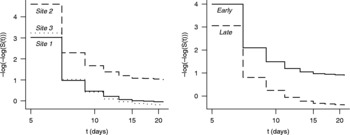
We suggest a model-building procedure similar to ones employed with ordinary multivariable regression models. As an initial exploratory technique, we suggest using a non-parametric method (e.g. Kaplan–Meier) to estimate and plot survivor functions for different values of the covariates, as shown in Figs 4 and 5 for three study sites and two collection dates in the Japanese knotweed data. Next, the PH assumption should be assessed for different values of the covariates, and any remedies required by clear violations should be applied. An example for the Japanese knotweed test data is shown in Fig. 6, where  versus log(t) is plotted for different study sites (left panel) and for early versus late collection dates (right panel), based on Kaplan–Meier survivor functions. These plots show no evidence of decisive crossing of the transformed survivor functions, so the PH assumption is plausible for all covariates. Potential multicollinearity of the covariates should also be assessed in the initial phase of analysis, using the same methods (e.g. variance inflation factor) that are used in standard multiple regression analysis (Ryan, Reference Ryan1997; Draper and Smith, Reference Draper and Smith1998; Montgomery et al., Reference Montgomery, Peck and Vining2001; Belsley et al., Reference Belsley, Kuh and Welsch2004; Kutner et al., Reference Kutner, Nachtsheim, Neter and Li2004).
Diagnostic plots for assessing the proportional-hazards assumption of the Cox model. Both panels show plots of  versus t, with t on a logarithmic scale. The left panel shows Kaplan–Meier curves for the three study sites, with data for all eight collection dates combined. The right panel shows curves for early and late collection dates (dates 1–4 and 5–8), with data for all sites combined.

For the model-building process, categorical covariates are coded using indicator variables, while quantitative covariates are used unchanged. For example, in the Japanese knotweed data, study site is categorical with three categories, so we may define two indicator variables, x 1 and x 2, as follows:

(Note that x 1 = x 2 = 0 implies that site = Carroll.) Collection date is a quantitative variable and therefore can be inserted in the Cox model as a single covariate, x 3. Model building begins by putting one covariate at a time into the Cox model and checking the reported p value for the null hypothesis that βi = 0. Covariates for which p is sufficiently small (e.g. p < 0.05) are candidates for use in building up a multivariable model. This is done in exactly the same manner as in ordinary multivariable regression, using an automatic selection procedure (though we do not advocate using these by themselves), the Akaike Information Criterion (AIC), p values and so forth. Interaction terms can also be added to the model, provided there is a meaningful basis for them. Ultimately, one arrives at a Cox model that may have multiple covariates in it, and the hazard ratios can be interpreted.
For the Japanese knotweed test data, a forward-selection procedure based on p values produces a final Cox model that includes all three covariates (x 1, x 2, x 3) but no pair-wise interactions. Table 3 summarizes the model, including the estimated values of coefficients β1, β2 and β3. The hazard function has the form

where covariates x 1 and x 2 are indicator variables for study sites Friends and Rising Sun, and x 3 is collection date.
Summary table of the final Cox model for the Japanese knotweed test data, as produced by R function coxph() in package survival. SE denotes the standard error

We illustrate interpretation of this model by considering the effect of study site Friends. (A complete interpretation of the model is provided in the supplementary material.) To assess the effect of study site Friends on germination time while controlling for (or removing) effects of collection date, we consider the ratio of the hazard function with x 1 = 1, x 2 = 0 and x 3 taking on any admissible value (in the numerator), to the hazard function with x 1 = x 2 = 0 and x 3 constrained to the same value as in the numerator (in the denominator). The resulting hazard ratio is

Choosing x 1 = 1 and x 2 = 0 for any x 3 implies that the numerator applies to the Friends site for any chosen collection date, while choosing x 1 = 0 and x 2 = 0 with the same value of x 3 implies that the denominator applies to the Carroll site for the same collection date. Thus, the hazard ratio in equation (15) indicates that for any given collection date, seeds from the Friends site have a hazard function for germination that is 0.28 times (28%) as large as the hazard function for seeds from the Carroll site. This shows that the slope coefficient for Friends implicitly specifies the effect of Friends relative to Carroll. Recalling equation (4), this result indicates that for any given collection date, the survivor function for seeds from Friends will be greater than the survivor function for seeds from Carroll, and therefore seeds from Friends will tend to germinate later than seeds from Carroll.
Both R and SAS include dedicated modules for implementing the Cox model. The main function in R is coxph() in the survival package; the main procedure in SAS is phreg. Code examples for R and SAS are provided in the supplementary material, along with an example illustrating all the steps in building a multivariate Cox model for the Japanese knotweed test data.
Including random effects
The non-parametric and semi-parametric methods we have considered until now assume that covariates have fixed effects. But just as in ordinary least-squares regression, it is often desirable to include a random effect in the Cox model. For reasons that are somewhat arcane, random effects are called frailty effects in time-to-event analysis.
The most common situation in germination studies where inclusion of a frailty effect may be desirable is where there are subgroups within treatment groups, such that seeds within a subgroup have approximately the same hazard function while seeds in different subgroups of a treatment group may have slightly different hazard functions. An example is experiments with replicates, where conditions experienced by seeds in the same replicate (e.g. the same Petri dish) may be more similar than those experienced by seeds in different replicates, resulting in random differences in germination properties among replicates. Another example is experiments in which the subgroups within treatment groups consist of seeds from the same individual plant, which might be more similar than seeds from different individual plants. This type of frailty is often called shared frailty, because all individuals in the same subgroup share the same level of frailty.
The most common method of including frailty in the Cox model is the same, regardless of the number of covariates. In the case of shared frailty with a single quantitative covariate, the Cox model for the i-th subgroup can be written as

where αi is the (random, unobserved) level of the frailty for the i-th subgroup. We assume that αi is sampled from some probability distribution but is constant over time.
Unlike the case in ordinary least-squares regression, the frailty effect is assumed to be multiplicative rather than additive, as equation (16) shows. This means that among individuals with the same value of covariate x, those in subgroups with αi > 1 are at increased risk of experiencing the event relative to those in subgroups with αi < 1. We therefore choose a distribution for the frailty effect that has a mean of 1 rather than 0, so that αi = 1 corresponds to ‘average frailty’. The most common choice is a gamma distribution, though any distribution defined on (0, ∞) and having mean 1 can be used if it is supported by software.
Frailty levels for subgroups or individuals are assumed to be sampled from a probability distribution and therefore typically are not estimated. Instead, we take the variance of the frailty distribution to be an unknown parameter to be estimated, and we test the null hypothesis that the variance parameter is equal to zero. If the null hypothesis is not rejected, then there is no strong evidence of variability in frailty levels and the frailty effect is not retained in the model.
As when building a multivariable Cox model without frailty, there is no single ‘best’ procedure for building a multivariable model that addresses frailty. We suggest the following modification of the above procedure for models without frailty. In the initial stage of model building, where fixed-effect covariates are included one at a time, a frailty term should be included along with each individual covariate. If the frailty term is found to be statistically significant in any of these cases, then there is evidence that it is important and it should be included in all further steps of the model-building process, regardless of the subsequent p values reported for the frailty term. On the other hand, if the frailty term is not found to be significant with any of the individual covariates, then it should no longer be considered in further steps of the model-building process.
Extra care must be taken with interpretation of hazard ratios in models that include a frailty effect. To see this, consider a shared-frailty Cox model with a single quantitative covariate x, and let αi denote the frailty level for subgroup i (e.g. a replicate). Then the hazard ratio HR for covariate value x+1 in subgroup i relative to covariate value x in subgroup j is

Clearly the hazard ratio depends on the frailty effects unless αi = αj. But as noted above, we typically will not have estimates of αi and αj. Therefore, we must work with the hazard ratio by assuming αi = αj (so the frailty effects disappear) and interpret it as the effect of a unit increase in the covariate based on two subgroups with the same level of frailty.
At the time of this writing, SAS does not provide built-in procedures or options for including frailty terms in Cox models. In contrast, the process is simple in R and is accomplished by using the frailty() function to specify a frailty term in the model formula of the coxph() function.
We will use the Japanese knotweed test data to illustrate the process of building a multivariable Cox model that includes a frailty term. (Additional details and code examples can be found in the supplementary material.) The Japanese knotweed data do not include replicates, but for purposes of illustration, we created artificial replicates as follows. Using an R script, we randomly assigned the 100 seeds in each of the 24 treatment groups (8 collection dates × 3 study sites) to 5 subgroups of 20 seeds each. These 120 subgroups (24 groups × 5 subgroups per group) were then uniquely labelled and treated as replicates.
Applying the modified model-building procedure outlined above to these data, the first step is to include the fixed-effect covariates in a Cox model one at a time, while also including a gamma-distributed shared-frailty term along with each individual fixed-effect covariate. Each of the 120 replicates is assumed to be subject to a separate gamma-distributed random effect that applies to all 20 seeds. We find that all three covariates have significant effects (p < 0.01 in all three cases), and that the frailty effect is highly significant (p < 0.000001 in all three cases). We therefore include the frailty term in all remaining steps of building the model. We then build a multivariable Cox model in the same manner as before. The final model is summarized in Table 4. The main difference from the model summarized in Table 3 is that the covariate representing the Rising Sun site is no longer included. Recall that the germination pattern for this site is similar to that at the Carroll Park site for later collection dates, and that the site slope coefficients in the model represent effects relative to Carroll Park. Thus, random variation among replicates results in a loss of ability to detect a difference between the Rising Sun and Carroll Park sites.
Summary table of the final shared-frailty Cox model for the Japanese knotweed test data, as produced by R function coxph() in package survival. SE denotes the standard error, Chisq denotes chi-squared (χ2), and df denotes degrees of freedom

Summary and discussion
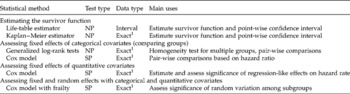
The various non-parametric and semi-parametric methods we have reviewed are summarized in Table 5. As can be seen by perusing this table, the most appropriate method depends on the questions of interest. If one is mainly interested in comparing groups of seeds, then non-parametric methods are an appropriate choice. In exchange for reduced statistical power, these methods have the advantage of avoiding any dependence on parametric assumptions. If one is interested in assessing effects of quantitative covariates on germination, such as temperature, duration of seed storage or duration of stratification (and possibly comparing groups, as well), then the semi-parametric Cox model is appropriate. Semi-parametric methods retain part of the advantage of non-parameteric methods by avoiding dependence on a fully parametric germination–time distribution, but the inclusion of covariates requires parametric regression-like assumptions about the form and strength of their effects. Fully parametric methods (not included in Table 5) are required only if one needs additional statistical power to detect small effects or wishes to quantify the shape of the survivor function in detail.
Summary of the major non-parametric and semi-parametric methods of time-to-event analysis supported by R and SAS
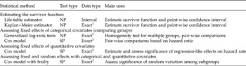
1 Ties are permitted; NP, non-parametric; SP, semi-parametric.
We have noted that data from germination experiments typically have two properties that differ from the norm in medical applications of time-to-event analysis for which most of the modern statistical methods were developed: a non-negligible initial delay in the onset of germination and an unknown mixture of germinable and non-germinable seeds. Implications of these properties regarding the validity or interpretation of the various methods of time-to-event analysis vary, as we now discuss briefly.
Neither of these properties of germination data affects the validity of non-parametric methods. They do, however, constrain the interpretation of any significant between-group differences that are detected, since the statistical methods do not indicate whether the detected differences are due to differences in initial delay, proportion of non-germinable seeds, some other aspect of the survivor function's shape or some combination of these properties.
Presence of an unknown proportion of non-germinable seeds does not affect the validity of the Cox model (Maller and Zhou, Reference Maller and Zhou1996), but in the same way as for non-parametric methods, it constrains the interpretation of any statistically significant covariate effects. The delay in onset of germination is potentially a more serious problem. The PH assumption cannot be strictly true in cases where the germination delay differs among experimental treatments. But as long as graphical assessment of the PH assumption does not indicate a clear violation, the Cox model will provide an acceptable approximation. The Japanese knotweed example illustrates this point well (see the supplementary material). If a clear violation of the PH assumption is evident, one can resolve the problem by simply removing the delay from the recorded germination times for each treatment before applying the Cox model. Otherwise, the delay should be retained.
In principle, neither the initial delay in onset of germination nor the presence of an unknown proportion of non-germinable seeds is problematic for fully parametric methods. As in the non-linear regression approach, these properties are represented by model parameters whose values must be estimated. But these properties are fatal problems if one wishes to analyse germination data with built-in functions or procedures of standard statistical software, because each implies a distribution of germination time that is not a member of the family of distributions permitted by current software (i.e. distributions that are members of the location-scale family for some differentiable and invertible transformation of germination time, such as log(T)). It is not difficult to construct appropriate distributions that include an initial delay and an unknown proportion of non-germinable seeds, but because such distributions are not accommodated by standard software, it is necessary to write custom code in order to estimate model parameters, construct confidence intervals and test hypotheses. Working within a statistical programming environment such as R makes these tasks reasonably straightforward, but the technical details are beyond the scope of this review.
Acknowledgements
The study from which our test data were taken was funded by a grant to J.N.M. from the William Penn Foundation; Margot Bram conducted the germination experiments. A.S. was supported by a D.J. Angus-Scientech Educational Foundation Internship at the Annis Water Resources Institute. Thanks to Roger Latham and the reviewers for helpful comments.