2.1. Governing equation

We consider a linearly stratified incompressible fluid and the corresponding Navier–Stokes equation under the Boussinesq approximation:

(2.1)$$\begin{gather} \partial_{t} \boldsymbol{u}+ \boldsymbol{\omega} \times \boldsymbol{u} + \boldsymbol{\nabla} p -\nu \nabla^{2} \boldsymbol{u}={b} \boldsymbol{z} + \boldsymbol{F}_{\boldsymbol{u}} \end{gather}$$

(2.2)$$\begin{gather}\partial_{t} b+\boldsymbol{u}\boldsymbol{\cdot}\boldsymbol{\nabla} b -\mathcal{X} \nabla^{2}b={-}N^{2} {u_z} . \end{gather}$$

The velocity vector is $\boldsymbol {u}=(u_x,u_y,u_z)$ with vorticity $\boldsymbol {\omega }=\boldsymbol {\nabla } \times \boldsymbol {u}$, and $p$ is the modified pressure field. The kinematic viscosity is $\nu$ and the thermal diffusivity $\mathcal {X}$. The Brunt–Väisälä frequency is $N$ so that the buoyancy field $b$ is the negative fluctuation of density around the mean constant gradient $N^2$. Here $\boldsymbol {z}$ is the unit vector of polar direction, also vertical. The flow can be set in motion via the body force $\boldsymbol {F}_{\boldsymbol {u}}$. All equations and parameters are dimensionless by reference to length and scale.

Our method for extracting the IGW from the full flow is based on the characteristics of IGWs. Indeed, classical IGWs are plane-wave solutions of the inviscid equations, obtained by removing the nonlinear terms of (2.1)–(2.2) and identifying their dispersion relation $\omega _r(\boldsymbol {k})$. However, in the presence of large-scale advection (such as the VSHF), this dispersion relation $\omega _r(\boldsymbol {k})$ is modified. If one only takes into account the sweeping effect by large structures on an IGW, assimilated to an advecting velocity field $\boldsymbol {c}$, the modification of the IGW characteristics can be modelled by the following linearized equations:

(2.3)\begin{equation} \left.\begin{gathered} \partial_{t} \boldsymbol{u}_G+ \boldsymbol{c} \boldsymbol{\cdot} \boldsymbol{\nabla}{\boldsymbol{u}_G} + \boldsymbol{\nabla} p_G -\nu_G \nabla^{2} \boldsymbol{u}_G=b_G \boldsymbol{z}\\ \partial_{t} b_G+\boldsymbol{c} \boldsymbol{\cdot}\boldsymbol{\nabla} b_G -\mathcal{X}_G \nabla^{2}b_G={-}N^{2} {u_{z,G}} + F_b \end{gathered}\right\} \end{equation}

and we shall use density forcing via $F_b$ with new variables named $\boldsymbol {u}_G, b_{G}, \nu _G$, $\mathcal {X}_G$ associated to (2.3). In our modelling of the modification of an IGW's characteristics, we do not take into account the refraction of waves by the vertical shear (i.e. $u_z{\partial _z c}$) as it does not significantly change our results: our DNS show that ${\partial _z c}\sim 0.04\ll N$, and the corresponding analytical evaluation and preliminary numerical tests show that the dispersion relation is not significantly modified in that case with respect to the sweeping effect.

The characteristics of the IGW are obtained by solving (2.3) and are used to extract the wave part from the full velocity obtained by (2.2). In both cases, it is useful to use the same basis of description for (2.2) and (2.3). In Fourier space, since incompressibility imposes that the velocity vector be perpendicular to the associated wave vector, we introduce polar-spherical coordinates, where the unit vectors of the so-called Craya–Herring frame are ($\boldsymbol {e}^t,\boldsymbol {e}^p,\boldsymbol {e}^k$) defined with respect to the vertical axis $\boldsymbol {z}$ as

(2.4a–c)\begin{equation} \boldsymbol{e}^t=\frac{\boldsymbol{k} \times \boldsymbol{z}}{|\boldsymbol{k} \times \boldsymbol{z}|}, \quad \boldsymbol{e}^p=\frac{\boldsymbol{k} \times (\boldsymbol{k} \times \boldsymbol{z})}{|\boldsymbol{k} \times (\boldsymbol{k} \times \boldsymbol{z})|}, \quad \boldsymbol{e}^k=\boldsymbol{k}/k . \end{equation}

Therefore, in this basis, the Fourier-transformed velocity writes $\hat {\boldsymbol {u}}(\boldsymbol {k},t)=\hat {u}^{t}(\boldsymbol {k},t)\boldsymbol {e}^t+\hat {u}^{p}(\boldsymbol {k},t)\boldsymbol {e}^p+\hat {\boldsymbol {u}}^{s}(k_z,t)$, where $\hat {\ }$ represents the Fourier transform in space (details in Lam et al. Reference Lam, Delache and Godeferd2020). The toroidal part $\hat {u}^{t}$ is horizontal and corresponds to a horizontal wave vector $k_h\ne 0$ with $k_h=(k_x^2+k_y^2)^{1/2}$, and the poloidal part $\hat {u}^{p}$ contains both horizontal and vertical velocity and thus corresponds to an IGW motion. In physical space, the corresponding velocity fields are $u^t$ and $u^p$. This decomposition excludes the VSHF mode– noted in Fourier space $\hat {\boldsymbol {u}}^{s}(k_z,t)=\hat {\boldsymbol {u}}(k_h=0,k_z,t)$ – which corresponds to the horizontal velocity field at an exactly vertical wave vector such that $k_h=0$. This results from the mathematical definition of polar-spherical coordinates based on an axis of symmetry borne by $\boldsymbol {z}$.

2.2. Method of extraction

In the original decomposition by Riley et al. (Reference Riley, Metcalfe and Weissman1981), the Craya–Herring decomposition is applied on velocity fields of stratified turbulence in the limit of small Froude number. The poloidal part $u^p$ is clearly the velocity of the IGW and the toroidal part $u^t$ is the non-wave part which coincides with a two-dimensional horizontally rotational velocity associated to eddy dynamics, and often called the ‘vortical mode’. This decomposition appears to be relevant at low-buoyancy Reynolds number $\textit {Re}_b \ll 1$ and at low Froude number $\textit {Fr} \ll 1$, where the flow consists of an interaction between vortical modes at large scale and an IGW (see Lelong & Riley Reference Lelong and Riley1991). At larger $\textit {Re}_b$, a part of vertical velocity $u^{p}$ and of density $b$ is linked to vertical mixing, and therefore not to waves. To account for this, Lam et al. (Reference Lam, Delache and Godeferd2020) extended Riley's decomposition to explicitly include the space–time properties of waves and their transport by a constant advecting velocity $\boldsymbol {c}$ estimated from the energy of the VSHF.

In the case of a constant advection velocity $\boldsymbol {c}$, homogeneous in time and space, Riley's decomposition applied to (2.3) is rigorous. Indeed, an analytical solution of Green's function of the IGW can be obtained from the linearized equations (2.3) forced by Dirac functions in time and space $F_b=\delta (t)\delta (x)$. Solved in the 4-D Fourier domain in space and time $(\boldsymbol {k},\omega )$, and denoted $\tilde {\ }$, Green's function of IGWs is composed only by the poloidal part denoted $\tilde {u}^p_{G,a}$ and by the density denoted $\tilde {b}_{G,a}$:

(2.5)\begin{equation} \left.\begin{gathered} \tilde{b}_{G,a}(\boldsymbol{k},\omega)=\frac{{1}}{2} \left\{ \left[{\mathcal{X} k^2+ \mathrm{i}(\omega+\omega_{c}^{+}(\boldsymbol{k}))}\right]^{{-}1} + \left[{\mathcal{X} k^2+ \mathrm{i}(\omega-\omega_{c}^{-}(\boldsymbol{k}))}\right]^{{-}1} \right \} \\ \tilde{u}^p_{G,a}(\boldsymbol{k},\omega)=\frac{\mathrm{i}}{2N} \left\{ \left[{\nu k^2+ \mathrm{i}(\omega+\omega_{c}^{+}(\boldsymbol{k}))}\right]^{{-}1} - \left[{\nu k^2+ \mathrm{i}(\omega-\omega_{c}^{-}(\boldsymbol{k}))}\right]^{{-}1} \right \} \end{gathered}\right\} \end{equation}

where the analytical dispersion relation $\omega _{c}^{\pm }(\boldsymbol {k}) = \boldsymbol {c} \boldsymbol {\cdot } \boldsymbol {k} \pm \omega _{r}(\boldsymbol {k})$ is $\omega _r$ modified to include $\boldsymbol {c} \boldsymbol {\cdot } \boldsymbol {k}$ that represents the sweeping effect, similar to Doppler shift. The toroidal part $\tilde {u}^t_{G,a}(\boldsymbol {k},\omega )$ is constant in time, i.e. with a zero frequency, and it is the vortical mode which is the rotational horizontal flow i.e. $k_h\ne 0$ (see note 14 in Smith & Waleffe Reference Smith and Waleffe1999). Our new technique is based on a filter $\zeta (\boldsymbol {k},\omega )$ in 4-D space $(\boldsymbol {k},\omega )$ applied on the density field $\tilde {b}$ and velocity field $\tilde {\boldsymbol {u}}$ from DNS. The wave part is obtained from the $\tilde {b}$ and $\tilde {\boldsymbol {u}}$ fields, and by filtering the frequencies $\omega$ associated with each wave vector $\boldsymbol {k}$ for the velocity component $\tilde {u}^{p}$ and density component $\tilde {b}$. In Lam et al. (Reference Lam, Delache and Godeferd2020), this filter is based on the analytical dispersion relation: $\zeta (\boldsymbol {k},\omega )=1$ when $\omega =\omega ^{\pm }_c(\boldsymbol {k})$, where $\boldsymbol {c}$ is horizontal and its amplitude $c$ varies in the range of $[-c_V,c_V]$, $c_V$ being the r.m.s. of VSHF amplitude. This supposes that at the large scale, such VSHF is modelled as a homogeneous flow that transports velocity fluctuations. In practice, the velocity of VSHF varies along the $z$-axis with time, i.e. $\boldsymbol {c}(z,t)$, and it is not possible to derive an analytical solution such as (2.5). More generally, no theoretical dispersion relation can easily be found when $\boldsymbol {c}$ is inhomogeneous. To overcome this difficulty we simulate numerically the Green function.

For an inhomogeneous advecting velocity $\boldsymbol {c}(z,t)$, we generalize a property that appears in the analytical wave solution (2.5): when the frequency $\omega \rightarrow \omega ^\pm _c(\boldsymbol {k})$, the density energy $|\tilde {b}_G|^2$ peaks, only damped by viscosity. This enables computation of the Green function relevant for the linearized equations (2.3), where $\boldsymbol {c}(z,t)$ is the inhomogeneous VSHF, numerically extracted from DNS i.e. $\hat {\boldsymbol {c}}(k_z,t)=\hat {\boldsymbol {u}}(k_h=0,k_z,t)$, and $F_b=\sum _{\boldsymbol {x},t} \delta (\boldsymbol {x}) \delta (t)$ is an inhomogeneous distribution of Dirac functions in space and time. The extended filter is obtained simply by computing the energy of $|\tilde {b}_G|^2$ with respect to the space variable $\boldsymbol {k}$ and time variable $\omega$. When the energy ${\tilde {b}}_G$ peaks, for $(\boldsymbol {k}_0,\omega _0)$, one defines the corresponding spectral region as characteristic of a wave, so we set $\zeta (\boldsymbol {k}_0,\omega _0)=1$. In practice, to reach the peak, the extended filter is therefore defined as

(2.6)\begin{equation} \text{if } |\tilde{b}_G(\boldsymbol{k},\omega)|^2 \geqslant \beta^{{-}1} \max_{\omega} |\tilde{b}_G(\boldsymbol{k},\omega)|^2 \text{ then } \zeta(\boldsymbol{k},\omega) = 1 \text{ else } \zeta(\boldsymbol{k},\omega) = 0 \end{equation}

where the real parameter $\beta =100$ is selected in order to capture all peaks of energy on a range of frequencies and take into account not only the spread of peak over frequencies due to diffusivity but inaccuracy due to spatial and temporal discretization (see § 3). The filter $\zeta (\boldsymbol {k},\omega )$ implicitly defines a new dispersion relation $\omega _G(\boldsymbol {k})$ that accounts for the inhomogeneity of $\boldsymbol {c}(z,t)$. It can be applied on the DNS fields to separate the wave part ($\zeta =1$, label ‘$w$’) from eddy part ($\zeta =0$, label ‘$e$’):

(2.7)\begin{equation} \left.\begin{gathered} {\tilde{\boldsymbol{u}}}^{w}(\boldsymbol{k},\omega)=\zeta(\boldsymbol{k},\omega) \tilde{u}^p(\boldsymbol{k},\omega)\boldsymbol{e}^p \\ {\tilde{\boldsymbol{u}}}^{e}(\boldsymbol{k},\omega)= \tilde{u}^t(\boldsymbol{k},\omega) \boldsymbol{e}^t + \left( 1 - \zeta(\boldsymbol{k},\omega) \right) \tilde{u}^p(\boldsymbol{k},\omega) \boldsymbol{e}^p \\ {\tilde{b}}^{w}(\boldsymbol{k},\omega)=\zeta(\boldsymbol{k},\omega)\tilde{b}(\boldsymbol{k},\omega) \quad \textrm{and} \quad {\tilde{b}}^{e}(\boldsymbol{k},\omega)=\left( 1- \zeta(\boldsymbol{k},\omega) \right) \tilde{b}(\boldsymbol{k},\omega) . \end{gathered}\right\} \end{equation}

In this decomposition IGWs are defined as being the poloidal and buoyancy components close to the dispersion relation. Eddies are defined here as elements that are not a wave like an IGW and that are not the VSHF either. In this article, we employ the term ‘eddy part’ for convenience, admitting that it is initially defined by what it is not. Nevertheless, the eddy part mostly contains large-scale vortical modes, which are exactly toroidal components, but also small-scale 3-D structures, which are a mixture of poloidal and toroidal components.

The decomposition of ${\tilde {\boldsymbol {u}}}^{w}$ agrees with the observations of Maffioli et al. (Reference Maffioli, Delache and Godeferd2020) that only the poloidal components recover the waves dispersion relation. The wave part in (2.7) contains only frequencies corresponding to the dispersion relation and the eddy part contains a part of vertical velocity and the density. Applying the inverse 4-D Fourier transform from frequency space $(\boldsymbol {k},\omega )$ to physical space $(\boldsymbol {x},t)$ yields $\boldsymbol {u}^a(\boldsymbol {x},t)=\sum _{\boldsymbol {k},\omega }\tilde {\boldsymbol {u}}^a(\boldsymbol {k},\omega ) \exp ({-\mathrm {i}\boldsymbol {k}\boldsymbol {\cdot }\boldsymbol {x}-\mathrm {i}\omega t})$, $b^a(\boldsymbol {x},t)=\sum _{\boldsymbol {k},\omega }\tilde {b}^a(\boldsymbol {k},\omega ) \exp ({-\mathrm {i}\boldsymbol {k}\boldsymbol {\cdot }\boldsymbol {x}-\mathrm {i}\omega t})$ ($a$ stands for $w$, $e$ and remaining part $s$), and one obtains the decomposition of velocity and density:

(2.8a,b)\begin{equation} \boldsymbol{u}(\boldsymbol{x},t)=\boldsymbol{u}^w(\boldsymbol{x},t)+\boldsymbol{u}^e(\boldsymbol{x},t)+\boldsymbol{u}^s(\boldsymbol{x},t) \quad \textrm{and} \quad b(\boldsymbol{x},t)=b^w(\boldsymbol{x},t)+b^e(\boldsymbol{x},t), \end{equation}

where the VSHF has been identified as a mean flow in physical space $\boldsymbol {u}^s(\boldsymbol {x},t)$ coming from its definition in Fourier space as $\hat {\boldsymbol {u}}^{s}(\boldsymbol {k},t)=\hat {\boldsymbol {u}}(k_h=0,k_z,t)$.

This decomposition enables defining an orthogonal basis and an inner product in vector function space, by using the complete set of unit vector functions $\textrm {e}^{\mathrm {i}\boldsymbol {k} \boldsymbol {\cdot } \boldsymbol {x}}$ and $\textrm {e}^{\mathrm {i}\omega t}$. For two functions $\hat {f}$ and $\hat {g}$, we thus define an inner product in terms of wavevector $\boldsymbol {k}$ and time $t$, as $[\,\hat {f}(\boldsymbol {k},t),\hat {g}(\boldsymbol {k}',t)] \equiv ({1}/{T}) \int _{T} \hat {f}(\boldsymbol {k},t) \overline {\hat {g}(\boldsymbol {k}',t)} \delta _{\boldsymbol {k}-\boldsymbol {k}'} \,\mathrm {d}t$, where $T$ is the considered time span and $\bar {\phantom {t}}$ is the complex conjugate. Due to the orthogonality of vector space functions and orthogonality of Fourier velocity with wavevector space $\boldsymbol {k}$ from incompressibility, one shows the orthogonality between wave, eddy and shear parts: $[\hat {b}^i(\boldsymbol {k},t),\hat {b}^j(\boldsymbol {k}',t)] \ne 0$ and $[\hat {u}^i_m(\boldsymbol {k},t),\hat {u}^j_n(\boldsymbol {k}',t)] \ne 0$ only if $i = j$ and $\boldsymbol {k}=\boldsymbol {k}'$ (where $i$, $j$ stand for $w$, $e$ or $s$; and $m$, $n$ stand for space direction $x$, $y$ or $z$). Moreover, the overall energetic content is $\langle \,\hat {f},\hat {g}\rangle =\sum _{\boldsymbol {k}} \textrm {Re}[\,\hat {f}(\boldsymbol {k},t),\hat {g}(\boldsymbol {k},t)]$.

3.1. Parameters space

In a first kind of DNS we run, (2.1) and (2.2) are solved using a standard pseudo-spectral algorithm in a 2${\rm \pi}$-periodic 3-D spatial domain. A phase shifting method is used to treat aliasing in the nonlinear term (see Lam et al. Reference Lam, Delache and Godeferd2020 for details). The Prandtl number is $Pr={\nu }/{\mathcal {X}}=1$. Ten numerical simulations have been run with the parameters shown in table 1 at resolutions of $256^3$ and $512^3$. The exploration of parameters is mainly based on $512^3$ points, the lower resolution of $256^3$ points is used to confirm and explore trends. We have plotted in figure 1 the exploration points in the parameter space $(\textit {Fr},\textit {Re}_b)$, along with data from Maffioli et al. (Reference Maffioli, Brethouwer and Lindborg2016) and Garanaik & Venayagamoorthy (Reference Garanaik and Venayagamoorthy2019). According to Brethouwer et al. (Reference Brethouwer, Billant, Lindborg and Chomaz2007), our parameters explore a VASF regime, which contains weak IGW interactions, where wave anisotropy extends to small scales ($\textit {Fr} \ll 1$ and $\textit {Re}_b\ll 1$), as well as a SST regime where the scale of wave anisotropy is distinct from small dissipative scales ($\textit {Fr} \ll 1$ and $\textit {Re}_b\gg 1$). The exploration of these two regimes also induce a modification of the Taylor-length-based Reynolds number $\textit {Re}_\lambda = u_{rms} \lambda / \nu$ with $\lambda$ the Taylor scale and $u_{{rms}}$ the r.m.s. velocity. The regimes studied in our numerical simulations and in other numerical simulations are shown in figure 1(a). The figure shows that the two resolutions of $256^3$ and $512^3$ explore different regions of parameters space $(\textit {Fr},\textit {Re}_b)$ and we expect this to change the characteristics of the transition regime between the VASF and SST regimes. Additional few points in parameter space at $256^3$ resolution enables exploration of a slight variation of $\textit {Re}_b$ and $\textit {Fr}$. The two parameters $\textit {Fr}$ and $\textit {Re}_b$ are of course dependent on one another since $\textit {Re}_b=Fr^2 Re_h$, via the horizontal Reynolds number $Re_h={u_h^4 / (\varepsilon _u \nu )}$, defined by Maffioli et al. (Reference Maffioli, Brethouwer and Lindborg2016), which accounts for the horizontal turbulence intensity. The $256^3$ simulations have almost one order of magnitude lower $\textit {Re}_h$ than the $512^3$ simulations (see table 1) for similar $(\textit {Re}_b,Fr)$. By adjusting the resolution, one can therefore study the variation of the dynamical system either by setting $\textit {Fr}$ and weakly increasing $\textit {Re}_b$ (from low to high resolution), or by setting $\textit {Re}_b$ and weakly increasing $\textit {Fr}$ (from high to low resolution) in the parameter map.

Table 1.

List of parameters in the seven DNS runs. Here $Re_h={u_h^4 / (\varepsilon _u \nu )}$ is the horizontal Reynolds number, $S_E$ is the ratio of energy of shear flow over the total kinetic energy, $D_E$ is the ratio of density of shear energy per point against the total kinetic energy per point, and $\omega _{{max}}={{\rm \pi} }/{ \Delta t'}$ and $\omega _{{min}}={2{\rm \pi} }/{T}$ are the maximum and minimum pulsation solved.

Figure 1.

(a) Our parameters of the numerical simulations (open circle for $512^3$ points and filled circle for $256^3$ points). For reference, the DNS of Maffioli, Brethouwer & Lindborg (Reference Maffioli, Brethouwer and Lindborg2016) (from $96^3$ points to more than $1024^3$ points) and Garanaik & Venayagamoorthy (Reference Garanaik and Venayagamoorthy2019) ($512^3$ points) are shown. (b) Total kinetic energy $E_u^T(t)$ and VSHF energy $E_{u}(k_h=0,t)$ for $\alpha =1$ and $\alpha =0$ for $\textit {Re}_b=5$ and $Fr=0.023$.

3.2. Numerical parameters

The time step $\Delta t$ varies with the stratification $N$ to agree with the Courant–Friedrichs– Lewy (CFL) condition. For the spatial resolution of $512^3$ points, the maximum wavenumber is $k_{max}=241$ such that $k_{max} \eta \sim 1.1$, $\eta$ being the Kolmogorov scale (see table 1). This moderate number of points is necessary because our wave/eddy decomposition requires many 3-D fields in time. Turbulence reaches a statistically stationary state due to the added body force $F_u$ in (2.1), as in Maffioli et al. (Reference Maffioli, Delache and Godeferd2020) who injected a constant power $P=\int \boldsymbol {F}_{\boldsymbol {u}}\boldsymbol {\cdot }\boldsymbol {u}\,\mathrm {d}v=10$. Here $\boldsymbol {F}_{\boldsymbol {u}}$ is spectrally localized on a cylindrical spectral surface of horizontal wavenumber $k_h=4$ and vertical wavenumber $1\leqslant k_z \leqslant 3$, away from the VSHF at $\hat {\boldsymbol {u}}(k_h=0,k_z)$. It forces the poloidal and toroidal parts of the velocity equally. Thus this choice allows on average the wave and vortex components of the flow (in the sense of Riley's decomposition) to be excited in equal proportions. The forced wavenumbers are at an angle $\theta _f$ between the wavevector $\boldsymbol {k}$ and the horizontal plane, in the range $0.72 \leqslant \theta _f \leqslant 1.31$, meaning that high frequencies close to $N$ are forced and a wave turbulence cascade may develop with lower frequency. To delay the emergence of VSHF at the large scale, we add a friction term $\hat {\boldsymbol {F}}_u-\alpha \hat {\boldsymbol {u}}({k}_h=0,k_z)$ (with $\alpha =1$) as proposed by Le Reun et al. (Reference Le Reun, Favier, Barker and Le Bars2017) to stabilize the geostrophic mode in rotating turbulence. The latter authors also note that this term mimics the effect of a horizontal wall. It also helps the numerical simulation to reach a stationary state, as shown in figure 1(b). This figure shows the total kinetic energy $E_u^T(t)$ and the kinetic energy of VSHF $E_u^T(k_h=0,t)$ for $\alpha =1$ and $\alpha =0$. Both energies diverge when $\alpha =0$ but stay bounded when $\alpha =1$. This statistical stationarity allows computation of time Fourier transforms with less truncation-related spurious effects. Furthermore the divergence of the kinetic energy $E_u^T(t)$ for $\alpha =0$ is approximately the same as that of VSHF energy $E_u^T(k_h=0,t)$, which means that roughly the same amount of energy is advected by the VSHF. The main difference between the two cases with and without friction is that the flow is significantly advected by VSHF in the first case ($\alpha =0$), whereas this advection is much less in the case with friction ($\alpha =1$).

Our simulations contrast with those of Maffioli et al. (Reference Maffioli, Delache and Godeferd2020) in that we apply a friction term to quench VSHF to less than a few percent of the total kinetic energy, though still active enough to contribute to the flow structuration. We show in table 1 that the percentage of shear energy over the total kinetic energy ($S_E=E_u^T(k_h=0,t)/E_u^T(t)$) is very low. However, we still consider the VSHF to be the main advecting flow.

We consider that all wavevectors $k_x$, $k_y$, $k_z$ ($512^3$ points) are ‘active’ – i.e. they are prone to contributing significantly – in the total kinetic energy, whereas in the kinetic energy of the VSHF, we only consider wavevectors with $k_h=0$ as active, at whatever $k_z$ ($512$ points). Then, from these total kinetic energy $E_u^T$ and kinetic energy of VSHF $E_u^T(k_h=0)$, it is possible to define the following average energy densities: $e_{{K}}={E_u^T}/{512^3}$ and $e_{{shear}}={E_u^T(k_h=0)}/{512}$. These average densities explicitly take into account the number of active wavenumbers they involve. Finally, we can define the average density ratio per wavevector by $D_E=e_{{shear}}/{e_K}$. The value $D_E$ is given in table 1 and shows the relative importance of the VSHF compared with the number of points in the DNS involved. Here $D_E\sim 1000$ shows that the VSHF importance per point is strong for weaker stratification, but decreases while still intense for higher stratification.

In a second kind of DNS we run in order to build the $\zeta$ function, in preparation for the DNS with $512^3$ points, Green's function is simulated during $T=10\,000\Delta t$ by using (2.3) with the forcing term $F_b=\sum _{\boldsymbol {x},t} \delta (\boldsymbol {x}) \delta (t)$, where each Dirac function is set at a random position and enforced at each time step $\Delta t$ during the first $100 \Delta t$. The initial condition of this calculation is zero. The velocity $\boldsymbol {c}$ comes from the VSHF $\hat {\boldsymbol {u}}(k_h=0,kz)$ extracted every $\Delta t'=10 \Delta t$ from the DNS, after it has reached statistical stationarity. To ensure that IGWs are not dissipated, we use very small viscosity $\nu _G=\mathcal {X}_G=10^{-8}$ and we check that only the poloidal part $\hat {u}^p$ and the density $\hat {b}$ are active with respect to the toroidal part $\hat {u}^t$ that is close to machine-precision zero. We apply the fast Fourier transform (FFT) in time on $1000$ fields of $\hat {b}_G$ extracted every $\Delta t'$. For DNS with $256^3$ points the time step $\Delta t$ can be taken as larger and results in a DNS with less iterations ($T={4000}$ or ${5000} \Delta t$) but with statistics written on the same time step $\Delta t'=0.002$ as in numerical simulations with $512^3$ points. The time step is chosen as very small in order to capture the sweeping effect from the full r.m.s. velocity $u_{rms}$ on the highest frequency of eddies $u_{rms}k_{{max}}$, as validated in homogeneous and isotropic DNS by Di Leoni, Cobelli & Mininni (Reference Di Leoni, Cobelli and Mininni2015). The highest frequency of eddies $u_{{rms}}k_{{max}}$ must be compared with the maximum frequency $\omega _{{max}}$ and minimum frequency $\omega _{min}$ resolved by the numerical algorithm. The fields are not extracted at every $\Delta t$ both to reduce the memory cost and because in the DNS this time step comes mainly from the CFL constraint.

The value $\beta =100$ is based on the simulation of Green's function under conditions similar to the analytical solution (2.5) for buoyancy $\tilde {b}_{G,a}$, which is a benchmark for our method. As explained after (2.6), $\beta$ is the cutoff parameter for identifying the spectral peaks. Two reasons render imprecise the capture of peaks in the simulation of Green's functions. First, even if very low (e.g. $\nu _G=\mathcal {X}_G=10^{-8}$), viscosity tends to smear the peaks around the resonance frequencies $\omega _c^{\pm }$. Spectral discretization also adds to this smearing: for each wavevector $\boldsymbol {k}$, 100 % of energy is localized in a single frequency $\omega _c^{\pm }({\boldsymbol {k}})$ when analytically computed, whereas it is distributed over a bandwidth of frequencies in simulations. The second reason is due to time discretization: the frequency $\omega _c^{\pm }$ is not exactly measured, but is approximated by the two closest discrete frequencies. These two mechanisms lead to a search for the set of points closest to the peak. When trying to capture the peak in a configuration similar to the analytical solution (2.5), we observe that the peaks span several orders of magnitude in amplitude over a bandwidth of frequencies. In simulations, even if 100 % of the energy is distributed over all frequencies, in practice a large percentage is still located in a small frequency range. In numerical simulations in the exact configuration of the analytical solution $\tilde {b}_{G,a}$, we adjust $\beta$ to $100$ because we observe that $95\,\%$ of the total potential energy is selected as waves around a small bandwidth of frequencies. This $95\,\%$ value is retained for all the simulations of Green's function from (2.3). Choosing lower $\beta$ means that less potential energy from (2.3) would be considered as waves, which means that some eddies would be assigned as waves. Conversely, choosing a higher $\beta$ would not change the wave energy in (2.3) much and might increase the number of eddies associated to the IGW. In configurations other than the analytical solution, simulations of Green's functions also show that more or less $95\,\%$ of the total potential energy is preserved as waves.

Eventually, the $\zeta$ filter is applied to the $\hat {u}^t,\hat {u}^p,\hat {b}$ fields extracted every $\Delta t '$ from the stationary part of the first type of DNS, i.e. over the same period $T$ of extraction of VSHF. The inverse FFT then yields the decomposition (2.8a,b). No Hann window is used to avoid modifying the signal and energy, except for the creation of $\zeta$. All following statistics are averaged over $T_0=600 \Delta t'$ in the middle of the time domain $T$. They do not change significantly if $T_0$ is halved, which ensures they are converged. All frequencies are adequately resolved since the minimum frequency is $\omega _{min}=2 {\rm \pi}/T$ and the maximum frequency is $\omega _{max}= {\rm \pi}/\Delta t'$. In the supplementary movie available at https://doi.org/10.1017/jfm.2021.589, the video compares the fields $b,b^w,b^e$ for $N=70$.

4.1. Energy of waves and eddies

The total mechanical energy $E^T=E_{u}^T+E_{b}^T$ is the sum of kinetic energy $E_{u}^T$ and potential energy $E_b^T$. Based on our orthogonal decomposition, we split these energies into their wave and eddy parts as $E^T=E^w+E^e$ and $E^l=E_{u}^l+E_{b}^l$, with $E_{u}^{l}= 0.5\langle \hat {\boldsymbol {u}}^l,\hat {\boldsymbol {u}}^l\rangle$ and $E_{b}^{l}=0.5 N^{-2} \langle \hat {b}^l,\hat {b}^l\rangle$, where $l$ stands for $w$ (wave), $e$ (eddy) or $T$ (total) and $\langle ,\rangle$ is defined in § 2. The eddy part of the poloidal kinetic energy is defined as $E^{p,e}=0.5\langle \hat {\boldsymbol {u}}^{p,e},\hat {\boldsymbol {u}}^{p,e}\rangle$.

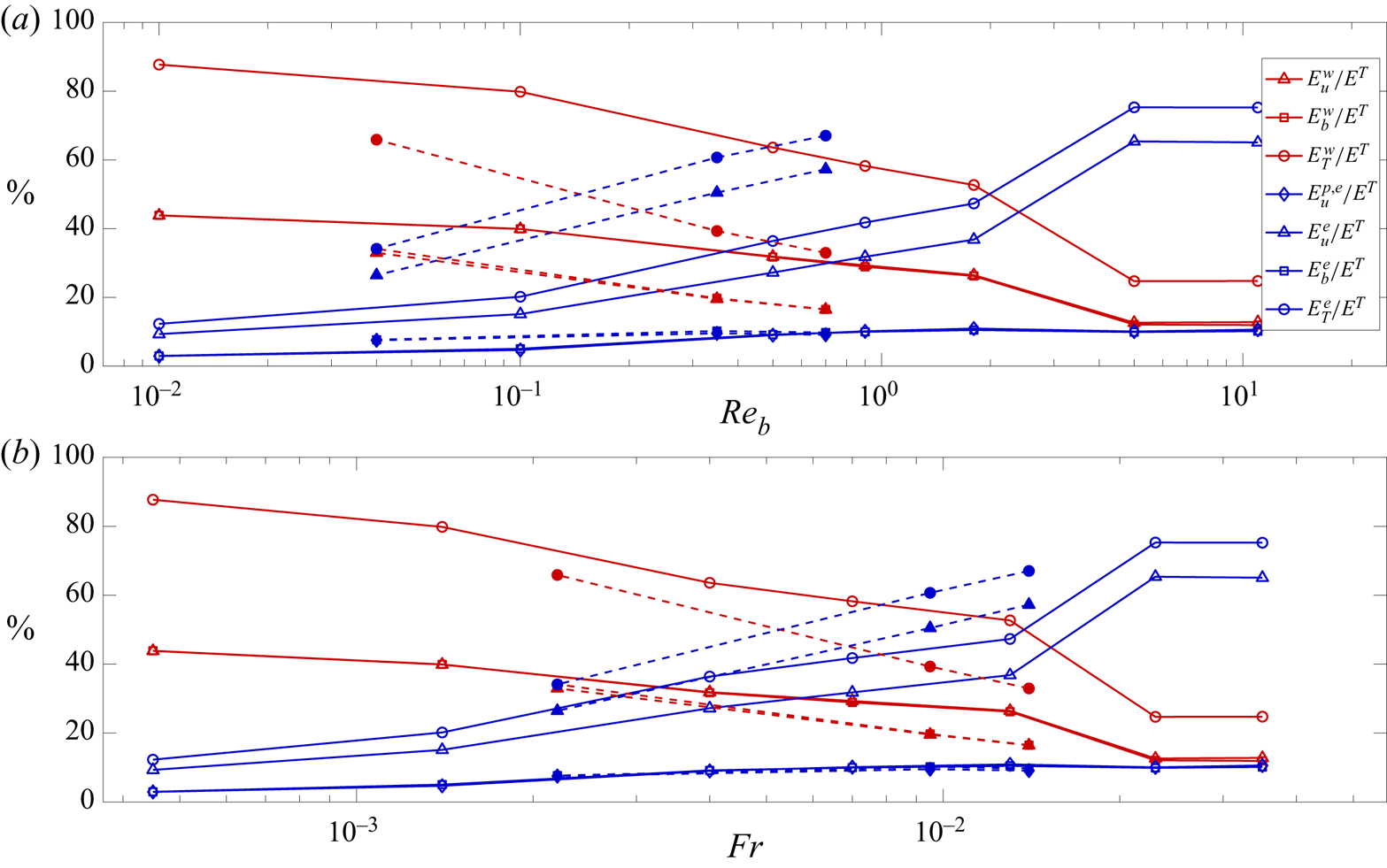
Figures 2(a) and 2(b) show for both resolutions, the energy distribution between waves and eddies, $E^e$ and $E^w$ compared with total energy $E^T$. Since two parameters $\textit {Fr}$ and $\textit {Re}_b$ appear to be strongly correlated (recall that $\textit {Re}_b=\textit {Re}_h \textit {Fr}^2$), we plot the distribution against $\textit {Fr}$ and $\textit {Re}_b$ separately. Moreover, we can observe the evolution of these energies either at constant $\textit {Re}_b$ and weakly increasing $\textit {Fr}$ (from high to low resolution on figure 2a), or at constant $\textit {Fr}$ and weakly decreasing $\textit {Re}_b$ (from high to low resolution on figure 2b). As expected, in figure 2 we observe that the eddy part of any form of energy $E^e$ increases and the wave part $E^w$ decreases, both when $\textit {Re}_b$ increases (figure 2a) and when $\textit {Fr}$ increases (figure 2b). Staquet & Godeferd (Reference Staquet and Godeferd1998) found a similar distribution of kinetic energy ($60\,\%$ to eddies and $40\,\%$ to waves) at $\textit {Fr} \simeq 0.006$ for decaying turbulence. Moreover, at fixed $\textit {Re}_b$ (figure 2a), when $\textit {Fr}$ increases, there is more energy in the eddy part than in the wave part, as expected by the meaning of $\textit {Fr}$ (inertial effects are more important than gravity effects). By increasing $\textit {Fr}$, the evolution of $E^w,E^e$ as a function of $\textit {Re}_b$ seems to be shifted to smaller values of $\textit {Re}_b$ as well as towards the equilibrium point where $E^w=E^e$. Nevertheless, at fixed $\textit {Fr}$ (figure 2b), when $\textit {Re}_b$ decreases, there is more energy in the eddy part than in the wave part, which is not obvious. Once again, this evolution seems to be shifted towards a smaller value of $\textit {Fr}$.

Figure 2.

Evolution of the percentage of energy in waves and eddies $(E_{i}^e/E^T,E_i^w/E^T)$ for kinetic, potential and total energy ($i=b,u,T$, respectively) against (a) $\textit {Re}_b$; (b) $\textit {Fr}$. Numerical simulations with $512^3$ points are shown with open symbols and solid lines, and numerical simulations with $256^3$ points are shown with filled symbols and dotted lines.

To analyse this result, we must analyse the composition of each type of energy. Figures 2(a) and 2(b) show the ratio of potential and kinetic energy distribution of waves $(E_b^w, E_u^w)$ and eddies $(E_b^e, E_u^e)$ to total energy $E^T$. First, we observe that the buoyancy energy $E_b^w$ and kinetic energy $E_u^w$ contain the same percentage of total energy of waves, i.e. $E_b^w \sim E_u^w$ for any $\textit {Re}_b$ or any $\textit {Fr}$, as generally expected for gravity waves. Second, we observe that the buoyancy energy of eddies is less than the kinetic energy of eddies i.e. $E_u^e > E_b^e$ for any $\textit {Fr}$ or $\textit {Re}_b$. Nevertheless, at fixed $\textit {Fr}$, for instance at $\textit {Fr} \sim 0.014$, when $\textit {Re}_b$ decreases there is more kinetic energy in the eddy for lower $\textit {Re}_b$ i.e. $E_u^e(Fr=0.014,\textit {Re}_b=0.7) > E_u^e(Fr=0.013,\textit {Re}_b=1.8)$.

This non-obvious result can be analysed by decomposing the kinetic energy of eddies into poloidal and toroidal parts. By following the decomposition (2.7) and (2.8a,b), the eddy part can be decomposed into poloidal and toroidal components: $E_u^e=E_u^{p,e}+E_u^{t,e}$ where $E_{u}^{p,e}=0.5\langle \hat {\boldsymbol {u}}^e \boldsymbol {\cdot } \boldsymbol {e}^{\boldsymbol {p}},\hat {\boldsymbol {u}}^e \boldsymbol {\cdot } \boldsymbol {e}^{\boldsymbol {p}}\rangle$ and $E_{u}^{t,e}=0.5\langle \hat {\boldsymbol {u}}^e \boldsymbol {\cdot } \boldsymbol {e}^{\boldsymbol {t}}, \hat {\boldsymbol {u}}^e \boldsymbol {\cdot } \boldsymbol {e}^{\boldsymbol {t}}\rangle$. In figures 2(a) and 2(b), we have only plotted $E_{u}^{p,e}$, from which the value of $E_{u}^{t,e}=E_u^e-E_u^{p,e}$ can be deduced. We observe the same percentage of total energy in the poloidal and buoyancy eddy energy, i.e. $E_b^e \sim E_u^{p,e}$ independently of $\textit {Fr}$ or $\textit {Re}_b$. This percentage increases slowly with $\textit {Re}_b$ or with $\textit {Fr}$. Note that the total potential energy $E_b^T=E_b^w+E_b^e$ is linked to the available potential energy (see § 14.1 in Davidson Reference Davidson2013). The available potential energy is a mechanical form of gravitational potential energy that stores the energy of an unstable density pattern i.e. the low- and high-density fluid parcels are not in equilibrium. While a part of this unstable configuration is related to the IGW ($E_b^w$), as the waves induce spatial variations of density fluctuation, the other part ($E_b^e$) contains, among other things, a density overturn (high density over low density). It seems that the equality $E_b^e \sim E_u^{p,e}$ reflects the effect of eddies in the vertical plane, which is directly related to the poloidal part of the velocity field. Since $E_b^e \sim E_u^{p,e}$ is more or less constant with $\textit {Re}_b$ at fixed $\textit {Fr}$, this means that only the toroidal part $E_u^{t,e}$ increases when $\textit {Re}_b$ decreases. The increase of $E_u^{t,e}$ leads to an increase of the total kinetic energy of the eddy part $E_u^e$. We remind that the toroidal part ($k_h\ne 0$) does not include the VSHF ($k_h=0$). Generally, large scales contain more kinetic energy than small scales dominated by the dissipation, so that the large-scale vortical modes are well represented by the toroidal part of the energy. We therefore argue that the relative increase – with respect to total energy – of the part of kinetic energy in the vortical modes can be associated with an increase in large, smooth and stable horizontal layers as the flow is increasingly more in the VASF regime by decreasing $\textit {Re}_b$, as in the nomenclature of Brethouwer et al. (Reference Brethouwer, Billant, Lindborg and Chomaz2007). This observation could explain the shift of the distribution of energy $E^w$, $E^e$ towards smaller $\textit {Fr}$ as $\textit {Re}_b$ decreases.

Note that at very large $\textit {Re}_b$, it seems that $E_u^{p,e} \sim E_b^e \sim E_b^w \sim E_u^w$. In the original decomposition by Riley, at large $\textit {Re}_b$ all the potential energy of eddies $E_b^e$ and the poloidal part of kinetic energy of eddies $E_u^{p,e}$ are wrongly assigned to the wave part (i.e. ${\sim }10\,\%$ for each part), thus inducing a departure by $40\,\%$ in comparison to our results: $+20\,\%$ of energy in IGWs and $-20\,\%$ of energy in eddies.

4.2. Flux of waves and eddies

The evolution of total energy in stratified turbulence is driven by the flux of energy as $\textrm {d} E^T / \textrm {d}t = P-\varepsilon _T$, where the total dissipation $\varepsilon _T=\varepsilon _u+\varepsilon _b$ with $\varepsilon _u=\nu \langle k^2\hat {\boldsymbol {u}},\hat {\boldsymbol {u}}\rangle$ and $\varepsilon _b=\mathcal {X} N^{-2} \langle k^2\hat {b},\hat {b}\rangle$. During the statistically stationary regime, the total energy stored is constant, so that $\textrm {d} E^T / \textrm {d}t =0$ and, for all stratification intensities, the output flux balances the input flux as $P \simeq \varepsilon _T$. The wave and eddy decomposition now allows one to address the question: how do wave- and eddy-related fluxes evolve with stratification?

We consider the equation of evolution of wave and eddy parts described by Verma (Reference Verma2019) as Lin-type equations, and hence that for total energy. We start with $\widehat {\text {2.1}}$ and $\widehat {\text {2.2}}$ as space Fourier-transformed equations (2.1) and (2.2). We also use the space Fourier-transformed decomposition of velocity and density (2.8a,b), and we project both $\widehat {\text {2.1}}$ and $\widehat {\text {2.2}}$ on the wave part using the inner products $[\widehat {\text {2.1}},{\hat {\boldsymbol {u}}^w(\boldsymbol {k},t)} ]$ and $[\widehat {\text {2.2}},{\hat {b}^w(\boldsymbol {k},t)}]$, and on the eddy part using $[\widehat {\text {2.1}},\hat {\boldsymbol {u}}^e(\boldsymbol {k},t)]$ and $[\widehat {\text {2.2}},\hat {b}^e(\boldsymbol {k},t)]$, relying on orthogonality properties noted in § 2. This yields four $(\boldsymbol {k},t)$-dependent equations for potential/kinetic energy and for the wave/eddy part. Balance equations are finally obtained by summing the potential and kinetic energies and using the spectral integration $\langle ,\rangle$:

(4.1)\begin{equation} \left. \begin{gathered} \textrm{d} E^{w} / \textrm{d}t = T_{ee}^{w}+T_{we}^{w} -\varepsilon_T^{w} +P^{w}\\ \textrm{d} E^{e} / \textrm{d}t = T_{ww}^{e}+T_{ew}^{e} -\varepsilon_T^{e} +P^{e} \end{gathered}\right\} \end{equation}

where $\varepsilon _T^{l}=\varepsilon _{u}^{l}+\varepsilon _{b}^{l}$, with $\varepsilon _{u}^{l}=\nu \langle k^2\hat {\boldsymbol {u}}^l,\hat {\boldsymbol {u}}^l\rangle$ and $\varepsilon _{b}^{l}=\mathcal {X} N^{-2}\langle k^2\hat {b}^l,\hat {b}^l\rangle$, is the total dissipation rate for each part $l=w,e$, the exchange term $T_{ij}^l=\langle \widehat {\boldsymbol {u}^{i} \times \boldsymbol {\omega }^{j} },\hat {\boldsymbol {u}}^{l}\rangle -N^{-2}\langle \widehat {\boldsymbol {u}^{i} \boldsymbol {\cdot } \boldsymbol {\nabla } b^{j}},\hat {b}^{l}\rangle$ and the injected power $P=P^w+P^e=10$ for each part $P^l=\langle \hat {\boldsymbol {F}}_{\boldsymbol {u}},\hat {\boldsymbol {u}}^l\rangle$. In (4.1), one neglects the interactions $T_{sj}^l$ of waves and eddies with VSHF because in our simulations these terms are small compared with others (for $N=100$, $T_{sj}^l\sim O (10^{-7} T_{ij}^l)$). As discussed by Verma (Reference Verma2019), triadic transfers are such that $T_{ij}^l=-T_{il}^j$ so that $T_{we}^w=-T_{ww}^e$ and $T_{ew}^e=-T_{ee}^w$. Here $T_{ij}^l$ is an energy exchange term between $l$ and $j$ parts, due to the interaction between the part $j$ ‘convected’ by part $i$ that exchanges energy with part $l$. Thus, $T_{ij}^j=0$ so that such terms are not net exchange terms, but are dynamically similar to convection terms, since they convey the modification of part $j$ by part $i$ that acts onto part $j$. For instance, $T_{ee}^{e}=0$ and $T_{ww}^{w}=0$ are respectively similar to a classical nonlinear transfer between eddies and to a nonlinear transfer between waves. In the statistically stationary regime, $\textrm {d} E^{w,e} / \textrm {d}t =0$ and the equilibrium of the fluxes is reached since all terms compensate one another.

Figures 3(a) and 3(b) show, for both resolutions, the evolution with $\textit {Re}_b$ and with $\textit {Fr}$ of the amount of the different terms in (4.1). Again, we can estimate the evolution of these values either at fixed $\textit {Re}_b$ and weakly increasing $\textit {Fr}$ (from high to low resolution) or at fixed $\textit {Fr}$ and weakly decreasing $\textit {Re}_b$ (from high to low resolution). In order to facilitate physical interpretation, we show a corresponding flux diagram (as known as Sankey's diagram) in figure 4 for $\textit {Re}_b=1.8$ and $\textit {Fr}=0.013$ to visualize quantitatively the energy flux from the injection $P$ to the two dissipations $\varepsilon ^w_T$ and $\varepsilon ^e_T$, either directly or indirectly by wave/eddy exchange terms $T_{ij}^l$. Each band represents a component of the balance of energy, with a width proportional to the energy flux it involves. Red, blue and cyan respectively indicate the wave, eddy and exchange parts.

Figure 3.

Evolution with (a) $\textit {Re}_b$ and (b) $\textit {Fr}$ of the contributions of forcing $P^l$, dissipation $\varepsilon ^l$ and transfer $T_{iw}^{e}$ from waves to eddies. The transfer from eddies to waves is easily computed as the inverse of the transfer from waves to eddies $T_{ie}^{w}=-T_{iw}^{e}$. Numerical simulations with $512^3$ points correspond to open symbols and solid lines, and numerical simulations with $256^3$ points to filled symbols and dotted lines.

Figure 4.

Sankey's diagram of energy flux at $\textit {Re}_b =1.8$ and $\textit {Fr}=0.013$ (see text).

Figures 3(a) and 3(b) show that at $\textit {Re}_b > \textit {Re}_b^T\simeq 2$ and $Fr>Fr^T\simeq 0.02$, the input power for waves and eddies is in balance exclusively with the dissipation, i.e. $P^e \simeq \varepsilon ^e_T$ and $P^w \simeq \varepsilon ^w_T$, and there is no exchange between waves and eddies. This does not mean that there is no transfer between waves and eddies, it only means that, overall, no net transfer occurs, but a scale-by-scale transfer (a ‘cascade’) is still possible between them. Moreover, injected energy is mainly pumped by eddies since $P^e > P^w$. This changes completely when $\textit {Re}_b$ decreases or $\textit {Fr}$ decreases as $\textit {Re}_b<\textit {Re}_b^T$ or $Fr< Fr^T$. Indeed, in the most stratified case $Fr=0.00045$ at low $\textit {Re}_b =0.01$, the input power and dissipation are more important for the wave part than for the eddy part ($P^w>P^e$ and $\varepsilon ^w_T > \varepsilon ^e_T$) and the exchange terms $T_{we}^w$ and $T_{ee}^w$ remove energy from waves ($P^w > \varepsilon ^w_T$) and redistribute it to eddies ($P^e < \varepsilon ^e_T$). As $\textit {Re}_b$ increases and $\textit {Fr}$ increases close to the transition $\textit {Re}_b \sim \textit {Re}_b^T$ and $Fr=Fr^T$, the dissipation associated with eddies gets larger ($\varepsilon ^e_T > \varepsilon ^w_T$) as expected but, surprisingly, the input power for waves remains large and there is a significant transfer from the wave part to the eddy part, which amounts to a total of up to 50 % of the eddy dissipation. During this transition, the exchange between wave and eddy is dominant. Similarly, Godeferd & Cambon (Reference Godeferd and Cambon1994) showed a lot of the energy appears to be pumped from the waves by the exchange term $T_{we}^{w}$. In this transition zone, at fixed $\textit {Re}_b$, when $\textit {Fr}$ increases, as expected, the eddy part takes more importance and the evolution seems to be shifted to a lower $\textit {Re}_b^T$. Nevertheless, by comparing the numerical simulations with $512^3$ points and $256^3$ points, it appears that the transfer mostly depends on the Froude number, although its amplitude varies slightly between the two resolutions. Moreover, the way the forcing and the dissipation is distributed between waves and eddies seems relatively invariant against the Froude number.

These observations result in a global analysis of transfers between waves and eddies: the global exchange is zero for the exchange terms, i.e. $T_{ee}^e= T_{ww}^w=T_{ew}^w=T_{we}^e=0$, but these terms are associated to ‘cascades’ and therefore influence indirectly the transfers between wave and eddies. For example, the global term $T_{ew}^w=0$, which means there is no global exchange, but there is still a scale-by-scale transfer between waves aided by an eddy that acts as a mediator (Verma Reference Verma2019).