


1. Introduction
The interaction between a vortex and the surface of an aerodynamic body is a ubiquitous phenomenon in unsteady and high-angle-of-attack aerodynamics, and is observed in a wide range of aerodynamic structures, including aggressively manoeuvring aircraft, blades on helicopter rotors and gas turbine engines and wind turbines (Ol & Gharib Reference Ol and Gharib2003; Bridges Reference Bridges2010; Mulleners, Kindler & Raffel Reference Mulleners, Kindler and Raffel2012; Yilmaz & Rockwell Reference Yilmaz and Rockwell2012). Robust models for prediction of aerodynamic loads or the application of flow control in massively separated flows require a better understanding of the underlying nonlinear dynamics and transport processes, which are currently not well understood. A vorticity transport framework provides a useful conceptual framework to understand and quantify some of the factors governing vortex growth. In the present work, the evolution of a leading-edge vortex (LEV) is investigated on a flat, rectangular plate of aspect ratio 2 that is articulated in a pure roll motion in the presence of a free stream. Volumetric particle image velocimetry (PIV) is employed, using a novel plenoptic imaging approach with a single high-resolution camera (plenoptic PIV), to provide quantitative measurements of the complex, three-dimensional flow fields. Vorticity fluxes contributing to the development and decay of the vortex are examined in the non-inertial frame, while varying advance ratio and the radius of gyration of the wing, to provide insight into the fundamental mechanisms governing vortex development.
2. Background
Leading-edge vortices are prevalent across a broad range of geometries and applications, from engineered aerodynamic bodies to natural swimmers and fliers. For an impulsively started airfoil at high angle of attack, Pitt Ford & Babinsky (Reference Pitt Ford and Babinsky2013) demonstrated that the LEV constituted the vast majority of the circulation around the body. Furthermore, Wojcik & Buchholz (Reference Wojcik and Buchholz2014a) showed that the circulation associated with the LEV on a low-aspect-ratio wing revolving in quiescent flow was significantly greater than that predicted by thin airfoil theory for equivalent translating sections corresponding to specific spanwise positions on the wing. (In the present context, the term revolving is used to describe a wing undergoing a starting rotation, in contrast to continuous spinning.) These observations support the common understanding that LEVs are a significant and often dominant repository of circulation in separated flows. In the latter case, cross-cancelation of LEV vorticity by entrainment of the secondary vortex was found to be a principal mechanism constraining LEV growth, and thus contributing to its stability on the wing (Wojcik & Buchholz Reference Wojcik and Buchholz2014b).
While not necessarily sufficient for achieving an attached vortex, cross-cancelation of LEV vorticity, due to entrainment of secondary (opposite-sign) vorticity into the vortex, is a robust phenomenon, and the diffusive flux of secondary vorticity from the surface of an airfoil has been shown to correlate directly with important events in the flow (Visbal & Shang Reference Visbal and Shang1989; Acharya & Metwally Reference Acharya and Metwally1992; Shih & Ho Reference Shih and Ho1994; Kuo & Hsieh Reference Kuo and Hsieh2001; Eslam Panah, Akkala & Buchholz Reference Eslam Panah, Akkala and Buchholz2015; Akkala & Buchholz Reference Akkala and Buchholz2017). For an airfoil in dynamic stall, Shih & Ho (Reference Shih and Ho1994) conducted an order-of-magnitude analysis of the vorticity balance on the suction surface, and demonstrated that the diffusive contributions are of the same order of magnitude as the convective contributions during the formation of the dynamic stall vortex. Indeed, Eslam Panah et al. (Reference Eslam Panah, Akkala and Buchholz2015) conducted measurements of the diffusive flux of secondary vorticity on a periodically plunging plate, and showed that it was approximately 50 % of that of the shear layer. They used time-resolved PIV measurements to reveal that the secondary vorticity was intermittently entrained by the leading-edge shear layer, resulting in cross-cancelation with the primary vortex. Onoue & Breuer (Reference Onoue and Breuer2017) used measurements of similar, entrained regions of secondary vorticity to estimate the rate of vorticity cross-cancelation on pitching swept and unswept wings, and found it also to be comparable to the shear-layer flux late in the formation of the LEV; much more significant than contributions due to axial flow in the vortex. Akkala & Buchholz (Reference Akkala and Buchholz2017) extended the analyses of Eslam Panah et al. (Reference Eslam Panah, Akkala and Buchholz2015) to explore the effects of three-dimensionality on a periodically plunging rectangular plate of aspect ratio 2, and showed that both spanwise convective fluxes and surface-diffusive fluxes were important to the regulation of vortex growth. In some instances, the combination of fluxes could actually reverse the vortex formation process at a given spanwise position.
The spanwise convective flux of vorticity, due to axial flow in the vortex, has also been surmised to drain vortex circulation and promote stability in several other studies (e.g. Ellington et al. Reference Ellington, van den Berg, Willmott and Thomas1996; Maxworthy Reference Maxworthy1981; Lentink & Dickinson Reference Lentink and Dickinson2009b). Jardin & David (Reference Jardin and David2014) showed that, for a revolving wing, axial flow in the LEV was primarily driven by spanwise gradients in the velocity of the wing. However, the role of spanwise flow on LEV stability, for revolving wings, is complex and does not appear to be well understood. For example, Birch & Dickinson (Reference Birch and Dickinson2001) found that blocking spanwise flow by applying chordwise fences to a revolving wing had little effect on vortex development. Lim et al. (Reference Lim, Teo, Lue and Yeo2009) showed that spanwise flow was usually observed on a swept wing, but it did not enhance LEV attachment. Rather, vortex stretching on a wing with curved leading-edge planform was found to delay LEV detachment. Similarly, Wong, Kriegseis & Rival (Reference Wong, Kriegseis and Rival2013) also observed little effect of spanwise flow on large-aspect-ratio swept wings (in which spanwise gradients were not present). However, Wong, laBastide & Rival (Reference Wong, laBastide and Rival2017) conducted a comparison of rotor-blade gust vs flapping-wing kinematics to show that spanwise flow on the wing could either strengthen or weaken the vortex, depending on the sign of the spanwise vorticity gradient. Chen, Wu & Cheng (Reference Chen, Wu and Cheng2019) investigated the starting rotation of an aspect-ratio 4 wing at  $Re=1500$, and observed that spanwise convection of vorticity was only significant relatively early in the rotation, and suggested that it may not be important for steadily revolving wings.
It is well established that wing rotation – as in the flapping motion of biological wings, or the spinning of compressor or propeller blades – can have a substantial effect on the development and stability of the flow over the body (Himmelskamp Reference Himmelskamp1947). In particular, the case of a wing revolving in a quiescent flow has been extensively investigated by several authors (Lentink & Dickinson Reference Lentink and Dickinson2009a; Kim & Gharib Reference Kim and Gharib2010; Carr, Chen & Ringuette Reference Carr, Chen and Ringuette2012; Ozen & Rockwell Reference Ozen and Rockwell2012; Bross, Ozen & Rockwell Reference Bross, Ozen and Rockwell2013; Garmann, Visbal & Orkwis Reference Garmann, Visbal and Orkwis2013; Wojcik & Buchholz Reference Wojcik and Buchholz2014b; Wolfinger & Rockwell Reference Wolfinger and Rockwell2015; Wong et al. Reference Wong, laBastide and Rival2017; Eldredge & Jones Reference Eldredge and Jones2019). Lentink & Dickinson (Reference Lentink and Dickinson2009b) argued that the Coriolis acceleration acted to increase spanwise flow, thus regulating the size and strength of the vortex by transporting vorticity to the wing tip and into the wake. Alternatively, Garmann et al. (Reference Garmann, Visbal and Orkwis2013) focused on the Coriolis force applied to the vortex, and found cases in which the direction of the force acted away from the wing surface, presumably aiding detachment, and was an order of magnitude less than that due to the pressure gradient.
The studies by Jardin & David (Reference Jardin and David2014, Reference Jardin and David2015) and Jardin (Reference Jardin2017) have greatly elucidated the role of Coriolis accelerations and other non-inertial phenomena. In a comparison between simulations of wings translating in uniform and revolving-wing-like shear flows, as well as a revolving wing in quiescent fluid, Jardin & David (Reference Jardin and David2014) showed that the spanwise flow was primarily driven by the shear-induced spanwise pressure gradient in the latter two cases, leading to prolonged attachment of the vortex. However, the revolving case – the only case including Coriolis and centripetal accelerations – yielded a more compact vortex positioned closer to the surface, and significantly greater forces than the other two cases, despite having slower circulation growth. Further analysis by Jardin & David (Reference Jardin and David2015) demonstrated that the non-inertial effects were, indeed, dominated by the Coriolis acceleration, and not centrifugal effects. Jardin (Reference Jardin2017) used a systematic sequence of simulations of a high-aspect-ratio revolving wing to demonstrate that the Coriolis acceleration contributes to both pressure gradients and spanwise flow, so that the phenomena are extensively connected and it is impossible to separate their specific effects. It should be noted that these studies focus primarily on Reynolds numbers of 500 or less, and Jardin (Reference Jardin2017) showed that the Coriolis effects may be somewhat weaker at higher Reynolds numbers.
In a recent review of the literature, Eldredge & Jones (Reference Eldredge and Jones2019) observed that LEV growth on revolving wings is stabilized primarily by a combination of Coriolis accelerations and vorticity annihilation over limited spanwise ranges. In an analysis of the vorticity budget, they also showed that, mathematically, the Coriolis acceleration makes a contribution to the vorticity transport equation analogous to tilting – which they dubbed, Coriolis tilting, and suggested that this non-inertial tilting effect contributed to a net weakening of the vortex by tilting surface-generated vorticity into a spanwise orientation with opposite sign to that of the primary vortex.
The radius of gyration  $R_g$ of a revolving wing affects the degree to which these rotational effects govern the flow. For example, Wolfinger & Rockwell (Reference Wolfinger and Rockwell2015) investigated the impact of varying radius of gyration of a wing revolving in quiescent fluid. A conical, coherent LEV was observed for
 $R_g / c = 1.7$ (where
 $c$ is the chord length of the wing); however, at larger radii of gyration, the LEV exhibited an arch structure over the outboard portion of the wing and eventually shed.
In contrast with the investigation of revolving wings in quiescent flow, and despite the broad application in turbomachinery, the development of LEVs on high-incidence revolving wings in the presence of a coaxial free stream has been largely unexplored. In addition to the investigation by Wong et al. (Reference Wong, laBastide and Rival2017) discussed above, a notable contribution was made by Bross et al. (Reference Bross, Ozen and Rockwell2013), who compared relatively rapidly revolving wings in a free stream with that in quiescent fluid. They showed that LEV development was not significantly affected by advance ratio (the ratio of streamwise progression to circumferential progression of the blade), over the range of values considered in their study, but the parameter did significantly affect the shedding of vorticity from the trailing edge. In a prior publication by the present authors (Johnson et al. Reference Johnson, Thurow, Wabick, Berdon and Buchholz2020), plenoptic PIV was employed to characterize LEV behaviour on a wing revolving in the presence of a free stream. For sufficiently small advance ratios (i.e. fast rotation), and low wing radius of gyration, an attached LEV was observed on the inboard portion of the wing. A vortex bifurcation was observed further outboard, which was located at a spanwise location dependent on advance ratio.
In the present work, we further examine the formation of LEVs on a wing revolving in a free stream using the same configuration investigated by Johnson et al. (Reference Johnson, Thurow, Wabick, Berdon and Buchholz2020). A detailed vorticity transport framework is used, which is formulated as a budget within a planar control region in a non-inertial reference frame attached to the wing. As with the model of Eldredge & Jones (Reference Eldredge and Jones2019), a Coriolis contribution is observed that bears resemblance to the vorticity tilting term, and its role in the transport framework is examined. Advance ratio and radius of gyration are varied – extending the range of advance ratios investigated by Bross et al. (Reference Bross, Ozen and Rockwell2013) – and the effects on vorticity fluxes governing the growth of the LEV are investigated.
3. Methods
A flat-plate wing was articulated in a pure rolling motion, at fixed pitch angle, within an oncoming uniform flow. Particle image velocimetry was conducted, using a novel plenoptic imaging system, to characterize the evolution of the LEV.
Experiments were conducted in the University of Iowa's free-surface water channel with test section width of 0.61 m, and water depth of 0.33 m. The water channel has flow conditioning consisting of an 8 : 1 contraction ratio, honeycomb and five screens to maintain free-stream turbulence intensity below 0.3 %. Free-stream velocity,  $U_{\infty}$, was held constant for all experiments, producing a chord-based Reynolds number of
 $Re_{c} = 10\,000$.
3.1. Wing configuration and parameters
The flat-plate wing was manufactured from acrylic to minimize laser reflections, and had a chord length,  $c= 76.3$ mm, span
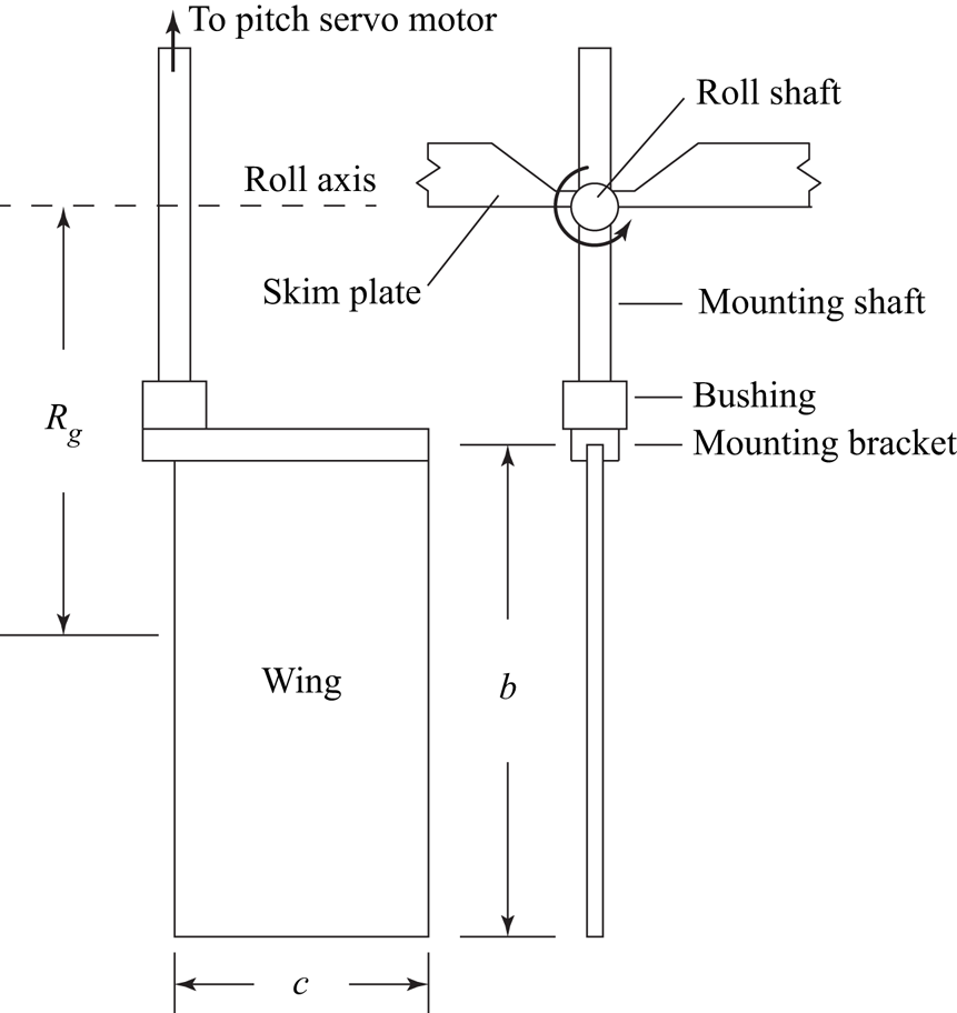
 $b= 152.6$ mm and thickness of 3.3 % of the chord, with both the leading and trailing edges rounded with a constant radius of half the plate thickness. A schematic of the wing is shown in figure 1. To ensure negligible deflection, the root of the wing was inserted into a stainless steel bracket extending the full chord length, and supported by an 8 mm diameter stainless steel mounting shaft at the leading edge. The shaft was attached to the bracket using a 19 mm outside diameter bushing, which facilitated the use of mounting shafts of different lengths in order to modify wing radius of gyration.
Schematic of the wing.

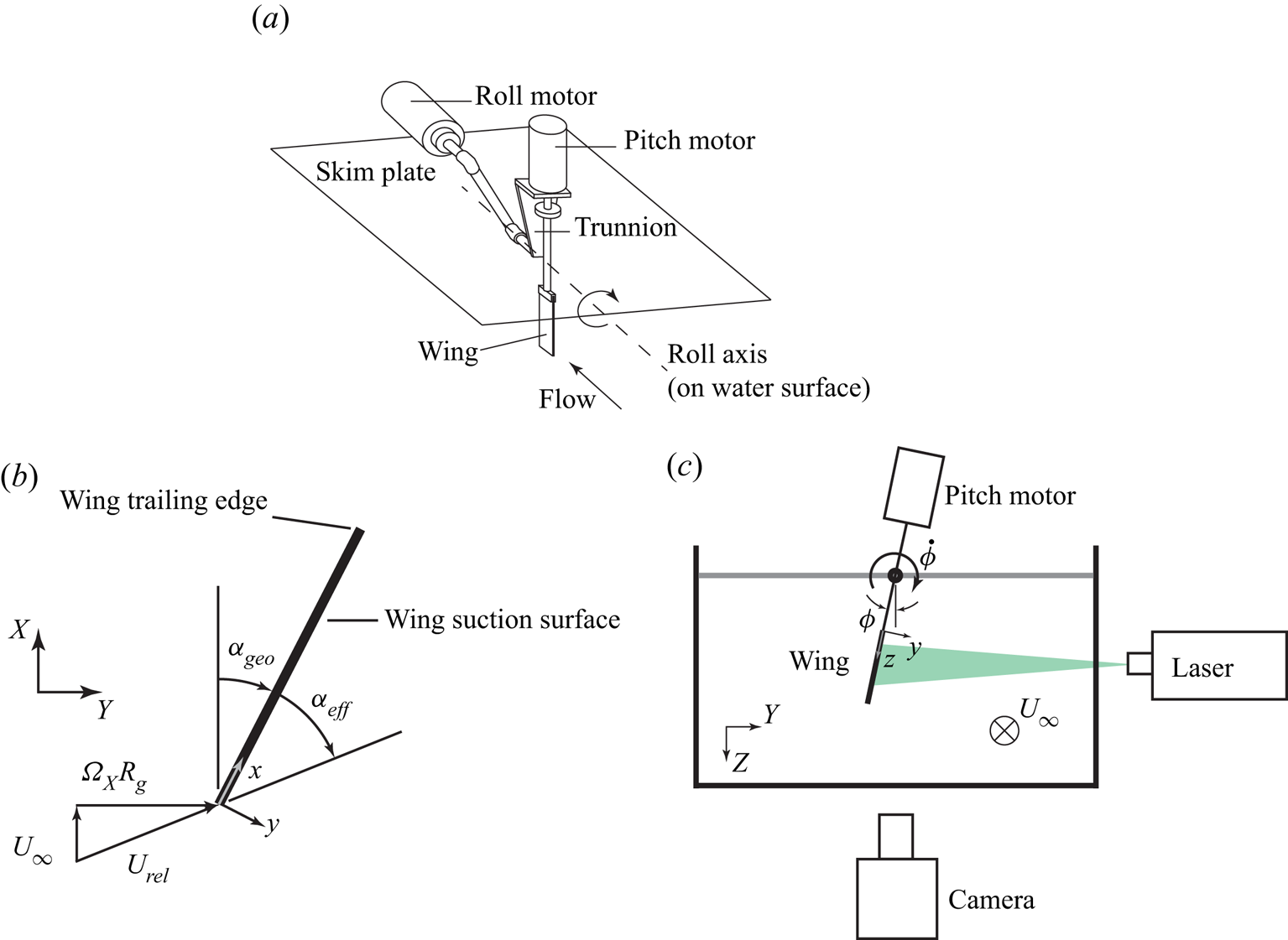
The wing was articulated in a roll manoeuvre about a roll axis aligned with the free stream, and coincident with the surface of a skim plate extending approximately 0.45 m upstream and 0.78 m downstream of the wing mid-chord. The roll motion was achieved using an Emerson XVM-8020-TONS-000 DC servo motor driven by an Emerson EP-204B servo drive and Galil DMC-4040 motion controller. A second servo motor, capable of articulating the wing in pitch, was installed on a rolling trunnion and was used in the present study only to maintain static pitch angles during experiments. The motion mechanism is shown in figure 2(a).
Experimental configuration and coordinate systems. (a) The motion mechanism; (b) angle and coordinate definitions (top view); (c) streamwise view of the experiment showing the orientation of the camera and laser illumination.

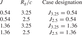
Four different combinations of kinematics and geometry were investigated by choosing two different values of advance coefficient,  $J=U_{\infty }/\dot {\phi }R_g = 0.54$ and 1.36, and two dimensionless radii of gyration,
 $R_g/c=3.25$ and 2.5 – a subset of the parameter values investigated by Johnson et al. (Reference Johnson, Thurow, Wabick, Berdon and Buchholz2020). Here,
 $R_g$ is the radius of gyration of the wing, and
 $\dot {\phi }$ is the roll rate. The wing was given a pitch angle
 $\alpha _{geo}$, specific to the roll rate and radius of gyration, such as to achieve an effective angle of attack
 $\alpha _{eff}=\alpha _{geo} + \arctan (\dot {\phi } R_g / U_{\infty })=33^{\circ }$. at the radius of gyration, as shown in figure 2(b). The wing was fixed at pitch angle
 $\alpha _{geo}$ prior to and during the roll motion. The roll displacement was prescribed as a linear ramp, smoothed using the Eldredge function (Eldredge, Wang & Ol Reference Eldredge, Wang and Ol2009) with a smoothing parameter of 1.2 and maximum roll angle
 $\phi _{max}=50^{\circ }$. The case in which
 $J=0.54$ and
 $R_g/c=3.25$ is considered the baseline case, and designated (
 $J_{3.25}=0.54$). The other combinations of
 $J$ and
 $R_g/c$ are similarly designated
 $J_{2.5}=0.54$,
 $J_{3.25}=1.36$ and
 $J_{2.5}=1.36$, as summarized in table 1.
Summary of rolling-wing cases considered in this paper, and their designations;  $J_{3.25}=0.54$ is referred to as the baseline case.

3.2. Plenoptic PIV
Three-dimensional velocity measurements were made using plenoptic PIV, which utilizes a light-field, or plenoptic, camera. Through the addition of a microlens array in between the main lens and the image sensor, a plenoptic camera gathers both spatial and angular information of a scene. This information, stored in the two-dimensional plenoptic image, is reconstructed into three-dimensional volumes. Akin to tomographic PIV, plenoptic PIV uses the multiplicative algebraic reconstruction technique (MART) to reconstruct the plenoptic images to volumes. The details of this process can be found in Fahringer, Lynch & Thurow (Reference Fahringer, Lynch and Thurow2015). Specific application of the method to the present data is detailed in Johnson et al. (Reference Johnson, Thurow, Wabick, Berdon and Buchholz2020), and summarized below.
Ensemble-averaged measurements were obtained at multiple angles. In order to simplify the imaging configuration, the wing was imaged with the spanwise axis in the vertical orientation for each case, requiring that the initial roll position of the plate was varied for each measurement angle. A modified 29 megapixel Imperx Bobcat B6620 CCD camera was used to record plenoptic images of the particle-laden flow field. The flow was illuminated using a  $200\ {\rm mJ}\ {\rm pulse}^{-1}$ dual-cavity Nd:YAG laser, which illuminated from the side of the water channel, pointing slightly upstream. The beam was spread into a volume using spherical and cylindrical lenses. The arrangement can be seen in figure 2(c). The right-handed non-inertial coordinate system for the measurement volume has its origin at the intersection of the wing root, leading edge and suction surface. The
 $+x$ direction is along the chord,
 $+y$ is normal to the wing and
 $+z$ is along the span towards the tip. A fixed (
 $X,Y,Z$) coordinate system is also defined, as shown in figure 2 such that the roll axis is parallel to the
 $X$-axis. Nearly the entire span of the wing was studied using 3 distinct measurement volumes, each centred at 20 %, 55 % and 89 % span, respectively. These planes are the nominal focal planes for each individual measurement volume. Each laser volume was masked in the
 $z$-direction before entering the water tunnel to extend
 $\pm 34$ mm from the nominal focal plane of and was clipped by the field of the view of the camera in the
 $x$ and
 $y$ directions, resulting in a volume with dimensions of
 $102\ {\rm mm} \times 68\ {\rm mm} \times 68\ {\rm mm}$ in
 $x$,
 $y$ and
 $z$, respectively.
To isolate the particle image data, reflections from the plate and other sources were removed through a proper orthogonal decomposition background subtraction method, described by Mendez et al. (Reference Mendez, Raiola, Masullo, Discetti, Ianiro, Theunissen and Buchlin2017). Each image was projected onto a basis where the most energetic modes from the larger data set were removed, representing repeatedly occurring light sources (Mendez et al. Reference Mendez, Raiola, Masullo, Discetti, Ianiro, Theunissen and Buchlin2017). For this study, the number of modes to remove was selected such that the change in normalized modal energy was less than the inverse of the total number of images in the phase data set. This resulted in approximately the 20 most energetic modes – corresponding to the most repeatable intensity patterns – being subtracted for each image.
Using 3 iterations of MART and a relaxation parameter of  $\mu = 1.0$, particle volumes were reconstructed onto a discretized grid of 527 voxels
 $\times$ 357 voxels
 $\times$ 357 voxels. An in-house three-dimensional cross-correlation algorithm was used (Fahringer et al. Reference Fahringer, Lynch and Thurow2015) with 5 passes of decreasing correlation volumes (64 , 48, 32, 16, 16 voxels and 50 % overlap) to produce vector fields of 63 vectors
 $\times$ 42 vectors
 $\times$ 42 vectors, with spatial resolution of 1.5 mm in each direction. Each vector field was then interpolated onto a grid such that the previously defined origin was located at the leading edge of the plate. The uncertainty of the measurements was quantified by measuring a free-stream flow, finding the uncertainty in velocity measurements as 2.3 %, 1.8 % and 4.0 % of the free-stream velocity for the velocities in the
 $x$,
 $y$ and
 $z$ directions (denoted
 $u_x$,
 $u_y$ and
 $u_z$), respectively.
4. Vorticity transport analysis
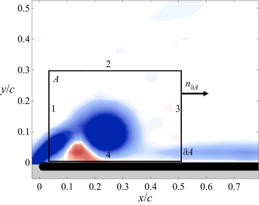
A circulation budget was constructed to track the sources and sinks of vorticity governing the strength of the LEV within a plane rectangular control region, as shown in figure 3. The control region extended from  $0.015 \leqslant x/c \leqslant 0.52$ and
 $0 \leqslant y/c \leqslant 0.30$, with the analysis conducted at multiple spanwise positions. The position and size of the control region were selected in order to closely encapsulate the LEV during its early development. However, it is important to note that the intention is not to characterize only evolution of the LEV, but also the growth of secondary vorticity within this very active region on the wing, in the interest of elucidating and quantifying the mechanisms that contribute to the overall circulation budget relevant to the LEV system. Therefore, the control region must be fixed to the wing surface and cannot conform to the shape of the LEV such that, in cases in which the LEV is shed, a significant quantity of circulation will cross the downstream boundary. Our approach is, therefore, to first characterize the integral contributions to the budget, then generate insight into the underlying physics by investigating the spatial distributions of the integrands and their constituent quantities.
Planar control volume in which the vorticity transport analysis was conducted. The plane area of the control region is designated  $A$, and has boundary
 $\partial A$, with outward-pointing normal
 $n_{\partial A}$.

Extending the analysis of Eslam Panah et al. (Reference Eslam Panah, Akkala and Buchholz2015) to include non-inertial accelerations due to rotation of the reference frame, the rate of change of circulation, with constant reference-frame angular velocity  $\boldsymbol {\varOmega }=( \varOmega _x, \varOmega _y, \varOmega _z)$, is given by
 \begin{align} \dfrac{{\rm d}\varGamma}{{\rm d}t} &={-}\int_{A_z}\left(u_z\dfrac{\partial {\omega_z}}{\partial {z}} \right) {\rm d}A - \oint \left({\boldsymbol{u}} \boldsymbol{\cdot} {\boldsymbol{n_{\partial A}}}\right)\omega_z \, {\rm d}s \nonumber\\ &\quad+ \dfrac{1}{\rho}\int_{bound~4} \dfrac{\partial {p}}{\partial {x}} \, {{\rm d}\kern0.06em x} + \int_{A_z}\left(\omega_x\dfrac{\partial {u_z}}{\partial {x}}+\omega_y\dfrac{\partial {u_z}}{\partial {y}} \right) {\rm d}A\nonumber\\ &\quad - \oint \left({\boldsymbol{u}} \boldsymbol{\cdot} {\boldsymbol{n_{\partial A}}}\right) 2\varOmega_z \, {\rm d}s + 2\oint_{\partial A} \left(-\varOmega_yu_z\,{{\rm d}\kern0.06em x} + \varOmega_x u_z\,{{\rm d} y} \right). \end{align}
The velocity and vorticity values presented in (4.1) are all represented in the non-inertial frame fixed to the rotating wing. The integrals are evaluated over the control-region area  $A_z$ or its boundary
 $\partial A$, which are illustrated in figure 3. The surface normal of
 $A_z$ is in the positive
 $z$-direction, which points to the root of the wing, and the in-plane normal to the boundary
 $n_{\partial A}$ is outward pointing, as illustrated in figure 3. The linear segments of
 $\partial A$ are numbered 1 through 4, with distinct behaviours of the transport terms expected on each. Boundary 1 tracks the shear-layer flux of vorticity into the control region, which is the primary source of negative vorticity feeding the LEV. Boundary 2 is placed above the vortex system such that it contributes little to the circulation budget. Boundary 3 captures fluxes due to convection of the boundary layer or a detached LEV structure, and is generally small in planes where an attached LEV is present. Finally, boundary 4 is adjacent to the surface of the wing, and captures the diffusive flux of vorticity due to pressure gradients created by the vortex system.
The non-inertial terms, which appear on the third line of (4.1), are derived in Appendix A. The first three terms on the right-hand side of (4.1) are readily interpreted in terms of physical convective and diffusive mechanisms. The first term describes the contribution due to the spanwise convective flux (i.e. convection of vorticity in the direction normal to the plane of the control region), and the second term describes the in-plane convection across the control region boundaries. The third term, which is only evaluated on boundary 4 (the surface of the wing), approximates the diffusive flux of vorticity from the surface. Diffusive and turbulent transport are neglected in this analysis, except on the surface of the wing (boundary 4), where diffusive transport dominates. The fourth term describes the contribution due to vortex tilting. Although vorticity tilting cannot affect the strength of a vortex tube surrounded by inviscid fluid, it can make a finite net contribution here due to the continuous distribution of vorticity and finite extent of the control region.
As noted in Appendix A, angular acceleration is absent during the measurements in this study, and centripetal accelerations make no direct contribution to the circulation budget. The two integrals in the third row of (4.1) represent the contributions due to Coriolis accelerations within the non-inertial frame. These terms are interpreted as corrections to the in-plane convection, and tilting contributions, respectively. For example, since the vorticity represented in the non-inertial frame comprises the actual vorticity present in the inertial ground reference frame, as well as the apparent solid body rotation corresponding to the rotational component of the non-inertial reference frame (the  $\omega _z$-component is relevant here, since the control-region normal is in the
 $z$-direction), the contribution to the second term of (4.1) made by the vorticity measured in an inertial reference frame would be
 \begin{equation} - \oint \left({\boldsymbol{u}} \boldsymbol{\cdot} {\boldsymbol{n_{\partial A}}}\right)\omega_z \, {\rm d}s - \oint \left({\boldsymbol{u}} \boldsymbol{\cdot} {\boldsymbol{n_{\partial A}}}\right) 2\varOmega_z \, {\rm d}s ={-} \oint \left({\boldsymbol{u}} \boldsymbol{\cdot} {\boldsymbol{n_{\partial A}}} \right)(\omega_z + 2\varOmega_z) \, {\rm d}s . \end{equation}
In accord with Eldredge & Jones (Reference Eldredge and Jones2019), application of Green's theorem to the second Coriolis integral yields a form analogous to the vorticity tilting term
 \begin{equation} 2\oint_{\partial A} \left(-\varOmega_yu_z\,{{\rm d}\kern0.06em x} + \varOmega_x u_z\, {{\rm d} y} \right) ={-}\int_{A_z} \left( 2\varOmega_x \dfrac{\partial {u_z}}{\partial {x}} + 2\varOmega_y \dfrac{\partial {u_z}}{\partial {y}} \right) {\rm d}A, \end{equation}
so that the net tilting contribution must take into account both the measured and Coriolis-tilting terms. It is noted that, while the physical tilting term represents actual tilting of free vorticity  $\boldsymbol {\omega }$, the Coriolis tilting term acts on the apparent vorticity induced by the rotation of the non-inertial frame,
 $2\boldsymbol {\varOmega }$, which is not amenable to reorientation by velocity gradients in the flow. With the interpretation of Coriolis accelerations as corrections to the measured fluxes in the non-inertial frame, they may be combined with the free-vorticity terms to represent net contributions to the circulation as observed in an inertial frame instantaneously coincident with the control region attached to the revolving wing
 \begin{align} &\int_{A_z}\left(\omega_x\dfrac{\partial {u_z}}{\partial {x}}+\omega_y\dfrac{\partial {u_z}}{\partial {y}} \right) {\rm d}A + 2\oint_{\partial A} \left(-\varOmega_yu_z\,{{\rm d}\kern0.06em x} + \varOmega_x u_z\, {{\rm d} y} \right) \nonumber\\ &\quad = \int_{A_z}\left((\omega_x + 2 \varOmega_x)\dfrac{\partial {u_z}}{\partial {x}}+(\omega_y + 2\varOmega_y)\dfrac{\partial {u_z}}{\partial {y}} \right) {\rm d}A, \end{align}
where the Coriolis-tilting term on the right-hand side is expressed using (4.3). For the purpose of elucidating the magnitudes of Coriolis-tilting contributions in the present framework, they will be presented separately, as given in (4.3).
In the present case of a pure rolling wing,  $\varOmega _z = 0$. Since the wing has a finite pitch angle, the non-inertial coordinate system is rolling about both the local
 $x$- and
 $y$-axes with roll rates
 $\varOmega _x = \dot {\phi } \cos \theta$ and
 $\varOmega _y = \dot {\phi } \sin \theta$.
5. Results
5.1. Flow structure
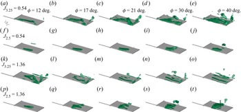
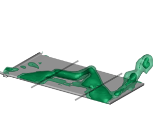
Figure 4 shows the evolution of the LEV for the four cases summarized in table 1, using the  $\lambda _{ci}$ (swirling strength) criterion (Zhou et al. Reference Zhou, Adrian, Balachandar and Kendall1999). The phase-averaged flows are visualized using isosurfaces of normalized swirling strength (
 ${\lambda ^2_{ci}}/{\textrm {max}\lambda ^2_{ci}}$) at values of 10 % and 15 %, following the guidelines given by Zhou et al. (Reference Zhou, Adrian, Balachandar and Kendall1999). Plenoptic PIV data were acquired over the entire span for the
 $J_{3.25}=0.54$ case, and subsets of the span for the others, to provide the breadth of parameter space presented here. The
 $J_{3.25}=0.54$ case is hereafter referred to as the baseline case.
The LEV formation shown with isosurfaces of normalized swirling strength levels of 0.10 and 0.25, for combinations of  $J=0.54$ and 1.36 and
 $R_g/c$=3.25 and 2.5, with
 $\alpha _{eff} = 33^{\circ }$. Each row depicts a different case; (a–e)
 $J_{3.25}=0.54$, (f–j)
 $J_{2.5}=0.54$, (k–o)
 $J_{3.25}=1.36$ and (p–t)
 $J_{2.5}=1.36$. Each column represents a specific roll angle comprising, from left to right,
 $\phi =12^{\circ }$,
 $17^{\circ }$,
 $21^{\circ }$,
 $30^{\circ }$ and
 $40^{\circ }$.

It should be noted that the wing mounting bracket, which thickens the wing along the root, will have some influence on the development of the LEV system. However, based on the visualization of the baseline case, it appears that the bracket has not substantially interfered with the formation of a conical LEV on the inboard portion of the wing.
Both of the  $J=0.54$ cases (
 $R_g/c=3.25$ and 2.5) exhibit an attached LEV on the inboard region of the wing, for the duration of the measurements, consistent with the observations of Bross et al. (Reference Bross, Ozen and Rockwell2013), for a similar advance ratio. The highest advance ratio investigated in that study was
 $J=0.537$, and the authors noted similar LEV development for lower advance ratios. For the baseline case, shown in figures 4(a) through 4(e), the inboard region is captured within the plenoptic imaging domain; whereas, for the wing with
 $R_g/c=2.5$, it is inferred because the most inboard portion of the imaged vortex remains stationary. This observation was also supported by dye visualizations (not shown).
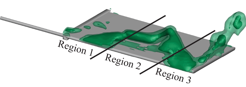
Furthermore, for the baseline case, three distinct behaviours can be observed across the span, as shown in figure 5. Region 1 ( $z/b\lessapprox 0.37$) is characterized by the attached, and essentially stationary LEV for the duration of the starting roll manoeuvre. In region 2 (
 $0.37 \lessapprox z/b \lessapprox 0.74$), the LEV separates from the wing, forming an arch structure, which sheds and is followed by the creation of subsequent vortices. By
 $\phi =30^{\circ }$, a second LEV structure is apparent, and a third is evident by
 $\phi =40^{\circ }$. In region 3 (
 $z/b \gtrapprox 0.74$), tip effects dominate, and the LEV structure reattaches and is pinned to the leading edge of the wing. A tip vortex is also formed.
Three distinct topological regions shown in the baseline case.

For the cases with  $R_g/c=2.5$ (figures 4f through 4j and 4p through 4t), data were acquired only along the central region of the wing (
 $0.35\leqslant z/b \leqslant 0.75$). The recorded region of the
 $J_{2.5}=0.54$ case also appears to support the existence of the two inboard regions (region 3 is not captured in the domain); however, unlike the baseline case, which exhibits sharp transitions between the three spanwise regions, the LEV structure transitions smoothly from the inboard attached structure to the separating structure at the mid-span (which is presumed to be a portion of an arch vortex displaced somewhat further outboard in comparison with the baseline case). The transition to a separating structure is most evident at
 $\phi =30^{\circ }$; whereas, it appears that, by
 $\phi =40^{\circ }$ the first LEV structure has advected downstream and dissipated as it is replaced by a second structure.
At  $\phi =12^{\circ }$, the
 $J=1.36$ cases exhibit structures similar to the
 $J=0.54$ cases at later times in their evolution. The measured flow structure for
 $J_{3.25}=1.36$ in figure 4(k) exhibits strong similarities to the
 $J_{3.25}=0.54$ case at
 $\phi =21^{\circ }$ (figure 4c). Similarly, the central region of the
 $J_{2.5}=1.36$ case, visible in figure 4(p), bears a strong resemblance to the
 $J_{2.5}=0.54$ case at
 $\phi =21^{\circ }$. Such observations of vortex-evolution delays governed by advance ratio have previously been made by Bross et al. (Reference Bross, Ozen and Rockwell2013) and Johnson et al. (Reference Johnson, Thurow, Wabick, Berdon and Buchholz2020).
5.2. Circulation distributions
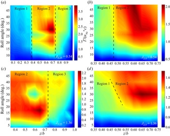
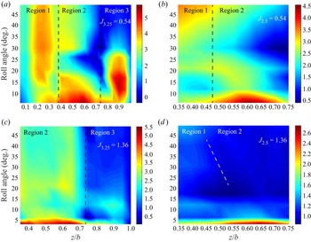
Figure 6 shows the variation in LEV circulation – measured within the control region illustrated in figure 3 – for the four rolling-wing cases. Circulation values were measured at  $\phi =6^{\circ }$,
 $12^{\circ }$,
 $17^{\circ }$,
 $21^{\circ }$,
 $26^{\circ }$,
 $30^{\circ }$,
 $40^{\circ }$ and
 $49^{\circ }$. at spanwise increments of 0.066
 $c$, and interpolated by a cubic spline using MATLAB's interp2 function on each spanwise plane. Approximate boundaries between regions 1, 2 and 3 – to the extent that they are included within the domains visualized in figure 6 – are depicted as dashed lines. All three regions are shown for
 $J_{3.25}=0.54$, whereas only regions 1 and 2 are evident for
 $J_{2.5}=0.54$ and
 $J_{2.5}=1.36$. Regions 2 and 3 are depicted for
 $J_{3.25}=1.36$. The boundary appears to move inboard for
 $J_{2.5}=1.36$; hence the sloped line in figure 6(d).
Spatial and temporal distribution of dimensionless circulation ( $\varGamma /(U_{\infty } c)$). The approximate boundaries between the regions defined in figure 5 are depicted here using dashed lines. In (a)
 $J_{3.25}=0.54$, all three regions are shown; in (b)
 $J_{2.5}=0.54$, regions 1 and 2 are shown; in (c)
 $J{3.25}=1.36$, regions 2 and 3 are shown; and in (d)
 $J{2.5}=1.36$, regions 1 and 2 are shown. Note the different spatial and circulation scales in each plot.

The three regions defined in § 5.1 exhibit distinct patterns of circulation growth tied to the disparate patterns of flow evolution found in these regions. For the baseline case, the circulation within region 1 grows slowly throughout the stroke (figure 6a). A striking transition in circulation is observed at the boundary between regions 1 and 2. In region 2, the maximum circulation observed is approximately double that in region 1, and exhibits two notable peaks at approximately  $\phi = 21^{\circ }$ and
 $30^{\circ }$, associated with the development of the second and third vortices. In contrast, in region 3, the circulation grows monotonically and remains relatively constant after approximately
 $\phi =25^\circ$.
It is not unexpected that the vortex strength within region 1 should be less than that further outboard, due to the lower velocity of the wing at inboard locations, and three-dimensional effects, which are further examined in § 5.4. Also, as discussed in § 2, it has been widely hypothesized, and demonstrated in some cases, that the conical vortex structure is stabilized by transport mechanisms that act to limit the circulation. Indeed, Jardin (Reference Jardin2017) observed, for a large-aspect-ratio revolving wing in quiescent flow, that the evolution in normal force was well represented by the sectional normal force at around 80 % span, demonstrating that a conical LEV attached to the inboard portion of the wing does not necessarily contribute a significant fraction of the lift.
Consistent with the observed flow structure behaviour, reducing the radius of gyration appears to decrease unsteadiness in the circulation, as the  $J_{2.5}=0.54$ case (figure 6b) exhibits more uniform circulation growth in time within the mid-span region of the wing. Similarly, figures 4(f) through 4(j) suggest that the vortex growth and shedding events occur over greater roll displacements. As with the baseline case, a sharp increase in circulation develops at approximately
 $z/b=0.47$, suggesting the transition from region 1 to region 2 delineated by the dashed line in figure 6(b), despite an apparently continuous variation in flow structure. It is also noteworthy that the location of this transition is further outboard on the wing than for the baseline case, consistent with the spanwise shift of LEV features observed in figure 4. While the tip region is not included in the
 $J_{2.5}=0.54$ measurement domain, it appears that the transition to region 3 would also occur further outboard.
For the  $J=1.36$ cases, the circulation distribution is aliased in time due to the rapid shedding of vortices from the leading edge. However, the data suggest spanwise variation in circulation that is roughly consistent with the fast-roll cases, despite that the measured values are somewhat arbitrary in these cases due to the advection of vorticity out of the downstream boundary. The spatial and temporal evolution of circulation for the
 $J_{2.5}=1.36$ case bears a strong qualitative similarity to
 $J_{2.5}=0.54$. However, an important distinction between the
 $J_{2.5}=0.54$ and
 $J_{2.5}=1.36$ cases is that, whereas the boundary dividing the low- and high-circulation regions (ostensibly regions 1 and 2) is stationary in the former, it moves inboard for the slow-roll (
 $J=1.36$) case as the motion progresses, as indicated by the slanted dashed line in figure 6(d). This indicates a destabilization of the inboard LEV in the slow-roll case, as would be expected for a translating wing in contrast to the fast-roll cases, where the LEV remains attached over the inboard region of the wing. This suggests that the existence of region 1 and its associated characteristics may not be caused by rotational effects, but merely prolonged by them. Data for the
 $J_{3.25}=1.36$ case are acquired to the tip of the wing, revealing a transition from region 2 to region 3 at approximately
 $R_g/c=0.7$, marked by the rapid drop in circulation. The location of this boundary is comparable to the baseline case, which indicates that the transition from region 2 to region 3 is due, primarily to tip effects, and not rotational effects.
5.3. Circulation budget closure and non-inertial contributions
Closure of the circulation budget described by (4.1) implies that the salient transport processes are adequately modelled, and that the measurements and derived quantities are sufficiently accurate. To assess the implementation of (4.1), spatial derivatives were evaluated using second-order central differencing of the plenoptic PIV velocity fields, and integrations were performed using the trapezoidal rule. The integral on boundary 4 of the control region was evaluated using pressure measurements acquired at  $z/b=0.5$ and chordwise positions of
 $x/c=0.015$ and
 $x/c=0.65$, employing the fundamental theorem of calculus.
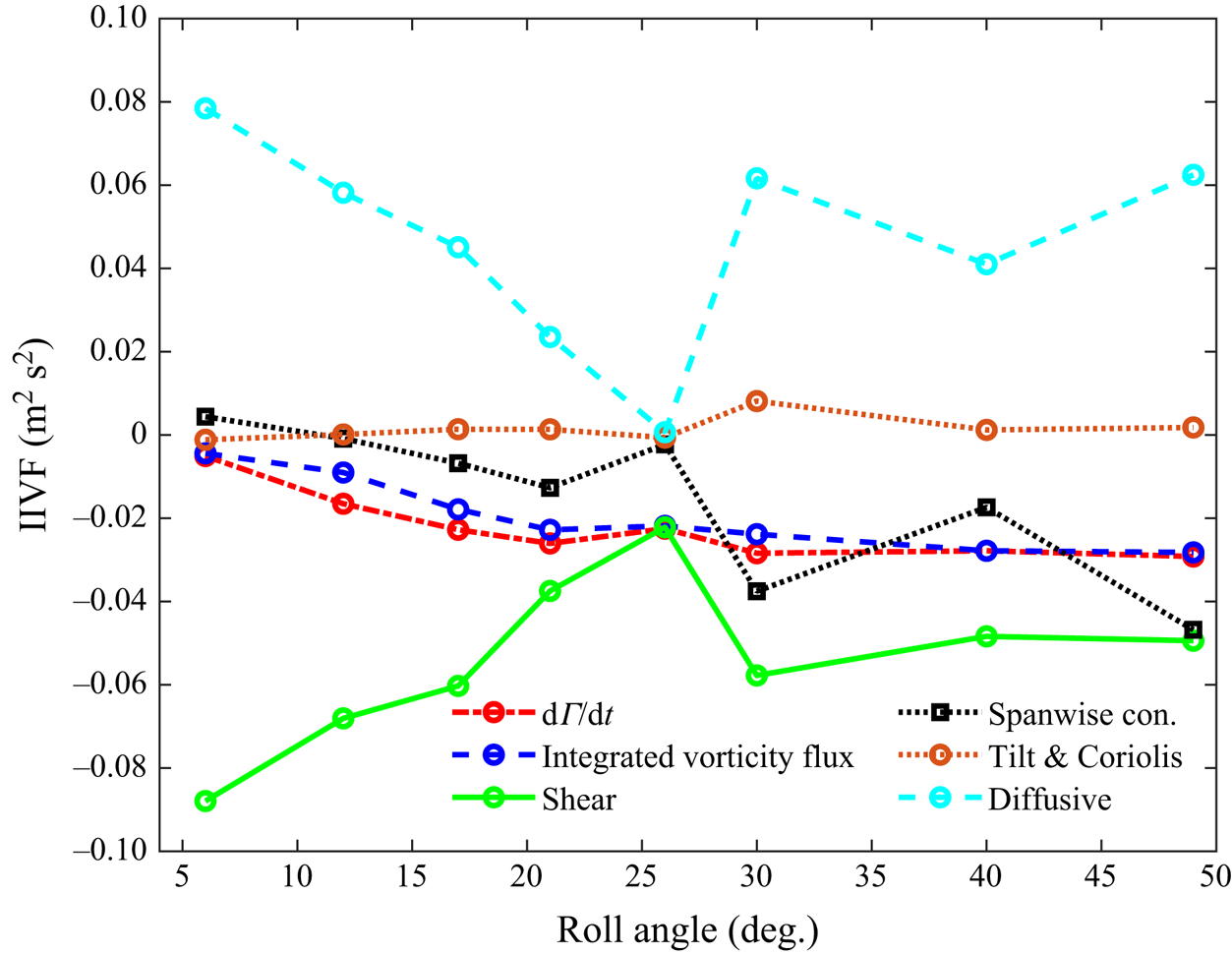
The terms on the right and left sides of (4.1), are plotted in figure 7 for  $J_{3.25}=0.54$ at the mid-span (
 $z/b=0.50$). The left side,
 $\mathrm {d}\varGamma /\mathrm {d}t$, is compared with the sum of the terms on the right side (designated ‘integrated vorticity flux’ in figure 7. Each of the terms on the right side of (4.1) are designated, generally, as instantaneous integrated vorticity fluxes (IIVF). The shear-layer flux through boundary 1 of the control region is labelled ‘shear’; whereas the combined contributions of tilting and Coriolis tilting are designated, ‘tilt and Coriolis’. The other terms on the right side of (4.1) include the spanwise convective flux and the diffusive flux through boundary 4. The computed rate of change of circulation (
 $\mathrm {d}\varGamma /\mathrm {d}t$) agrees well with the sum of the terms on the right-hand side of (4.1), indicating that the transport mechanisms governing control-region circulation are adequately described by (4.1). Based on this agreement, for other planes and cases, the diffusive flux on boundary 4 will be computed directly from (4.1), using plenoptic PIV data to obtain the remaining terms, and assuming equality.
Vorticity flux distribution for  $J_{3.25}=0.54$ at
 $z/b=0.5$.

Figure 7 shows that the dominant contributions to the circulation within the control region at  $z/b=0.5$ are the leading-edge shear layer and the surface diffusive flux on the surface of the plate. The shear-layer contributions in all cases are composed solely of measurements of the velocity field in the non-inertial frame, and do not include the Coriolis contributions. However, the distinction is practically unimportant in this case since the Coriolis contribution to the in-plane convective flux is negligible (i.e.
 $2\varOmega \ll \text {typical}$ values of
 $\omega _z$ in the shear layer). It should be noted that the sign of the vorticity in the shear layer and LEV is primarily negative; hence the negative circulation contribution of the shear layer.
The diffusive flux is opposite in sign, and thus strongly regulates the total circulation as the shear-layer contribution continues throughout the stroke. Notably, the contributions due to the tilting and Coriolis terms remain small in comparison with those of the dominant fluxes. Their negligible contribution to the circulation budget will later be shown to be robust across other spanwise locations and kinematic cases.
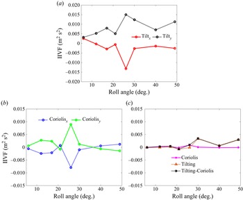
Figure 8 further examines the  $x$- and
 $y$-components of the physical and Coriolis-tilting contributions. Figure 8(a) shows that the spatial integral of
 $x$- and
 $y$-tilting terms (i.e. the separate integrals of
 $\omega _x \partial u_z/\partial x$ and
 $\omega _y \partial u_z/\partial y$, respectively) within the control region exhibit a highly symmetric behaviour as the roll angle progresses, resulting in substantial cancellation of their contributions to the circulation within the control region. This was also observed by Wojcik & Buchholz (Reference Wojcik and Buchholz2014b) for a wing revolving in quiescent fluid. The Coriolis tilting, shown in figure 8(b), behaves similarly. The net contributions of each of the tilting and Coriolis terms, as well as their sum is presented in figure 8(c). It is evident that the magnitudes of the net Coriolis and physical tilting contributions are indistinguishable within the measurement uncertainties.
Coriolis and tilting fluxes, integrated over the control region, for  $J_{3.25}=0.54$ at
 $z/b=0.5$; (a)
 $x$- and
 $y$-tilting terms (
 $\omega _x \partial u_z/\partial x$, and
 $\omega _y \partial u_z/\partial y$), (b) corresponding Coriolis terms (
 $2\varOmega _x \partial u_z/\partial x$, and
 $2\varOmega _y \partial u_z/\partial y$) and (c) a comparison between tilting and Coriolis contributions, as well as the net values of combined tilting and Coriolis contributions.

5.4. Vorticity transport analysis on the baseline ( $J_{3.25}=0.54$) case

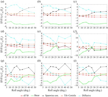
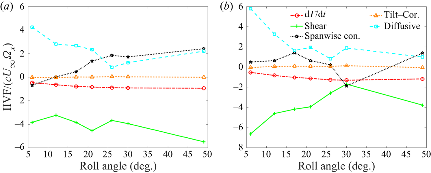
In this section, we will develop an understanding of the transport mechanisms governing the evolution of the LEV system circulation by considering the baseline case in detail. Figure 9 presents the contributions to the circulation budgets at nine spanwise locations on the wing. The data for  $z/b=0.20$ to 0.30 (figure 9a–c) reside in region 1;
 $z/b=0.40$ to 0.60 (figure 9d–f) reside in region 2; and those for
 $z/b=0.80$ to 0.90 (figure 9g–i) reside in region 3. Note that figure 9(e) contains data presented in figure 7. Data are presented as dimensionless vorticity fluxes (
 $IIVF/c U_{\infty }\varOmega _x$).
Vorticity transport budget for  $J_{3.25}=0.54$. Data are shown for region 1 (top row; (a)
 $z/b=0.20$, (b)
 $z/b=0.25$ and (c)
 $z/b=0.30$), region 2 (middle row; (d)
 $z/b=0.40$, (e)
 $z/b=0.50$ and (f)
 $z/b=0.60$) and region 3 (bottom row; (g)
 $z/b=0.80$, (h)
 $z/b=0.85$ and (i)
 $z/b=0.90$).

Justified by the circulation budget closure demonstrated in § 5.3, the diffusive-flux contribution, from the surface of the wing is inferred from (4.1) after computing the values of the other terms. Since the in-plane convective fluxes through control-region boundaries 2 (top) and 3 (downstream) are negligible in the present case, the shear-layer flux through boundary 1 is the main contribution to the in-plane convective term, and is labelled, shear layer. The tilting term is computed according to (4.4), and combines the physical and Coriolis tilting contributions.
At each of the spanwise locations represented in figure 9, the rate of circulation growth  $\mathrm {d} \varGamma / \mathrm {d}t$ is generally negative (LEV strength increasing in time) and significantly smaller than the magnitudes of the dominant flux contributions in each case, reflecting that circulation growth within the control region is the result of competing sources and sinks of vorticity. However, the transport processes exhibit striking differences in each of the three regions. The distinct transport characteristics of each region are examined in detail below.
5.4.1. Region 1
The shear-layer flux is the source that drives the growth of the LEV. In region 1 (figure 9a–c), the shear-layer contribution is substantially balanced by the diffusive flux from the wing surface early in the rotation. However, with increasing roll angle, the diffusive flux diminishes, and is replaced by a monotonically growing spanwise convective flux as centrifugal pumping on the wing surface begins to develop. As noted in § 2, some prior studies have measured a significant spanwise convective flux on revolving wings (e.g. Wong et al. Reference Wong, laBastide and Rival2017) while others have not (Wojcik & Buchholz Reference Wojcik and Buchholz2014b; Onoue & Breuer Reference Onoue and Breuer2017).
Thus, the region 1 data illustrate that the importance of the spanwise convective flux is time dependent. For a wing of aspect ratio 3 and root cut-out of 1 chord length, rotating in quiescent fluid, Chen et al. (Reference Chen, Wu and Cheng2019) found that spanwise convection was not significant until after approximately  $22^{\circ }$ of rotation, but diminished again after about
 $90^{\circ }$ of rotation. In the present experiments, the growth of the spanwise convective flux appears to have similar timing; however, there was not sufficient displacement to investigate whether spanwise convection diminished in the longer term. It should be noted that Chen et al. (Reference Chen, Wang, Zhou, Wu and Cheng2022) found that the importance of spanwise convective flux diminished significantly when Reynolds number reduced from
 $Re_c=1500$ to 100.
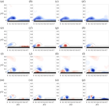
To understand the physical processes that govern the growth of the spanwise convective flux in region 1, figure 10 shows the distribution of spanwise vorticity, as well as the integrand of spanwise convective flux ( $u_z \partial \omega _z / \partial z$) and its constituent quantities. These include spanwise velocity (
 $u_z$) and the derivative of the vorticity in the spanwise direction (
 $\partial \omega _z / \partial z$), for
 $z/b=0.3$. With increasing progression in time, figures 10(a) through 10(d) show that the vortex becomes more diffuse, and its development begins to regress; descending toward the surface, reattaching to the downstream boundary layer, and decreasing in size. The start of this regression is concurrent with appearance of a strong outboard flow in the core of the vortex, evident in figures 10(f) and 10(g), and concomitant growth of the integrated spanwise convective flux observed in figure 9(c).
The LEV formation and components of the spanwise convective flux (spcf) at  $z/b=0.3$. Panels (a) to (d) depict the LEV evolution of the vorticity field. Panels (e) to (h) show the spanwise velocity distributions. Panels (i) to (l) show distributions of
 $\partial \omega _z / \partial z$. Finally, panels (m) to (p) show the spanwise convective flux distributions (
 $u_z \partial \omega _z / \partial z$). The columns represent roll angles of
 $\phi =17^{\circ }$,
 $21^{\circ }$,
 $26^{\circ }$ and
 $30^{\circ }$ from left to right.

Notably, the spanwise flow in the LEV core also diminishes abruptly between  $\phi =26^{\circ }$ and
 $30^{\circ }$ (figure 10g,h). However, as figure 9(c) shows, the integral contribution of the spanwise convective flux does not diminish, but merely persists with a modest growth rate. This is understood by considering the evolution of the vorticity gradient in figures 10(i) through 10(l), which grows monotonically, within the LEV, throughout the manoeuvre. Significant values of
 $\partial \omega _z / \partial z$ develop not only in the core of the LEV, but also in the attached boundary layer downstream of the control region (
 $x>0.52$). Despite the complex variability of the spanwise velocity, the spanwise vorticity gradient is correspondingly modulated in order to maintain a smoothly varying spanwise convective flux that mitigates the decline of the diffusive flux. This suggests that the transport features observed here are driven by constraints imposed by the global flow dynamics.
5.4.2. Region 2
In contrast to region 1, the spanwise convective flux is relatively insignificant throughout the roll motion in region 2 (figure 9d–f), and the circulation budget is dominated by a balance between the shear-layer and surface-diffusive fluxes. This behaviour is characteristic of planar motion of a nominally two-dimensional wing (e.g. Shih & Ho Reference Shih and Ho1994; Eslam Panah et al. Reference Eslam Panah, Akkala and Buchholz2015).
A brief reduction in the magnitudes of both the shear-layer and diffusive fluxes occurs around  $\phi =26^{\circ }$. To better understand the cause of this fluctuation, figure 11 shows the corresponding evolution of the spanwise vorticity field at
 $z/b=0.5$. At
 $\phi =26^{\circ }$ (figure 11c), the phase-averaged LEV begins to become diffuse, and the region of secondary vorticity, which has grown in size during the manoeuvre, starts to weaken and atrophy. The atrophy is likely due to entrainment of the secondary vorticity layer into the shear layer, as observed by Eslam Panah et al. (Reference Eslam Panah, Akkala and Buchholz2015). The existence of a significant accumulation of secondary vorticity is in distinct contrast to region 1 where, as figure 10 shows, it is essentially non-existent. A second LEV is forming at
 $\phi =30^{\circ }$ and
 $z/b=0.50$ (figure 11d) where figure 9(e) shows that the shear-layer flux has recovered.
Spanwise vorticity ( $\omega _z$) at
 $z/b=0.5$, (a)
 $\phi =17^{\circ }$, (b)
 $\phi =21^{\circ }$, (c)
 $\phi =26^{\circ }$, (d)
 $\phi =30^{\circ }$, (e)
 $\phi =40^{\circ }$ and (f)
 $\phi =49^{\circ }$.

5.4.3. Region 3
The flow field is highly three-dimensional in region 3, and exhibits flow evolution and flux contributions that are very different from regions 1 and 2. As noted in § 5.2, region 3 is characterized by tip effects and appears to be relatively insensitive to rotation. As figures 12(a) through 12(d) show, over time, the vortex evolves into a rapidly reattaching shear layer, suggesting that a strong favourable pressure gradient develops late in the manoeuvre. This is supported by the vorticity transport budgets for region 3, illustrated in figures 9(g) through 9(i), which show a strong diffusive contribution of negative vorticity by approximately  $\phi =40^{\circ }$. Until approximately
 $\phi = 25^{\circ }$, the shear layer is the primary source of LEV circulation. Its eventual weakening and concomitant favourable pressure gradient are plausibly connected with the development of the tip vortex.
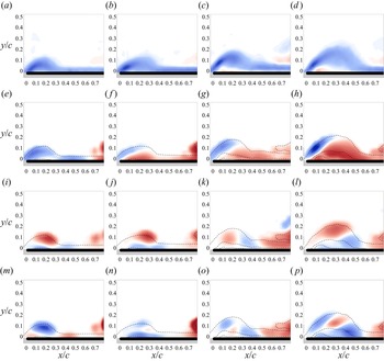
The LEV formation and components of the spanwise convective flux (spcf) at  $z/b=0.9$. Panels (a) to (d) depict the evolution of the vorticity field. Panels (e) to (h) show the spanwise velocity distributions. Panels (i) to (l) show distributions of
 $\partial \omega _z / \partial z$. Finally, panels (m) to (p), show the spanwise convective flux distributions (
 $u_z \partial \omega _z / \partial z$). The columns represent roll angles of
 $\phi =21^{\circ }$,
 $26^{\circ }$,
 $30^{\circ }$ and
 $40^{\circ }$ from left to right.

The spanwise convective flux also evolves concurrently with the shear-layer and diffusive fluxes. There is a characteristic drop in its magnitude around  $\phi =25$ to
 $30^{\circ }$, which corresponds to the drop in diffusive flux observed in region 2 during the formation of the second LEV, again suggesting that the three regions do not evolve independently. Similarly to the diffusive contribution in region 2, the spanwise convective contribution in region 3 subsequently recovers.
As with region 1, the persistent contribution of the spanwise convective flux can be further understood by examining its spatial distribution, as well as that of its constituents, as shown in figure 12 for  $z/b=0.90$. At
 $\phi =21^{\circ }$ (figure 12e), the spanwise flow in the vicinity of the LEV and adjacent boundary layer is inboard (blue). An inboard flow persists in the shear layer near the leading edge, throughout the manoeuvre, whereas a region of outboard spanwise flow is apparent at
 $\phi =26^{\circ }$, and grows in size with increasing roll angle. The outboard flow is predominantly located near the wing surface, and is likely driven, in part, by the tip vortex. Interestingly, the distribution of spanwise vorticity gradient is roughly complementary to the spanwise flow (i.e. positive values of
 $\partial \omega _z / \partial z$ are approximately coincident with negative values of
 $u_z$, and vice versa), such that the spanwise convective flux produces positive contributions to the net circulation within the shear layer, and adjacent to the wing surface. Similar to region 1, the patterns of spanwise flow and vorticity gradient are quite complex.
5.5. The role of radius of gyration and advance ratio
The previous section established characteristic patterns of vorticity transport in region 1, where an attached LEV was observed and rotational accelerations were important, and in region 2, where rotational accelerations appeared to be relatively unimportant. Lentink & Dickinson (Reference Lentink and Dickinson2009a) showed that the influence of rotational accelerations is inversely related to the Rossby number, which they expressed as  $Ro=U^2/(\varOmega ^2 R_g c)$ for a wing or blade spinning in a free stream. In terms of the advance ratio, this may be expressed as
 $Ro = [(R_g/c)(1 + J^2)]^{-1}$, such that the effects of rotational accelerations are reduced when both radius of gyration (
 $R_g/c$) and advance ratio are increased. Thus, as either parameter increases, we might expect the vorticity transport characteristics to tend toward region 2 behaviour and, conversely, with decreasing parameter values, transport flux behaviours characteristic of region 1 might become more prominent. In this section, we test this hypothesis by considering the three additional cases listed in table 1, in which
 $J$ and
 $R_g/c$ are varied.
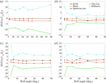
Figure 13 shows the vorticity transport budget for the  $J_{2.5}=0.54$ case at
 $z/b=0.35$ and 0.60. These spanwise locations are ostensibly within regions 1 and 2, respectively, considering the outboard shift of LEV features in comparison with the baseline case. Figure 13(a) shows that the primary transport attributes of region 1 are robust as radius of gyration is reduced. Specifically, the diffusive flux forms a significant contribution to the overall budget early in the manoeuvre, but is diminished later, as the spanwise convective flux increases. Again, tilting fluxes (physical and Coriolis) are negligible. The visualizations in figure 4 indicate diminished unsteadiness and complexity in the mid-span region, for the
 $J_{2.5}=0.54$ case, in comparison with the baseline case. Similarly, the evolution of the vorticity fluxes at
 $z/b=0.60$ (figure 13b) lacks the significant fluctuations in shear-layer and diffusive fluxes that are evident in the baseline case (figure 9d–f). A notable difference for
 $J_{2.5}=0.54$ is that, with the exception of the early part of the motion (i.e.
 $\phi <15^{\circ }$), the spanwise convective flux – while exhibiting oscillations, as in the baseline case – is generally of similar magnitude to the diffusive flux in the mid-span region of the wing (figure 13b). While this was also observed in the outboard portion of region 2 for the baseline case (figure 9f), the shear-layer and diffusive fluxes were generally dominant over the majority of region 2. Thus, with reduction of the radius of gyration, the distinction between regions 1 and 2 appears to be somewhat obscured, as spanwise transport remains significant in the mid-span region for
 $J_{2.5}=0.54$, supporting our hypothesis on the effect of reducing radius of gyration. Furthermore, the correlation between spanwise convective transport and the relative stability of the LEV persists in this region.
The vorticity transport budget for  $J_{2.5}=0.54$, at (a)
 $z/b=0.35$, and (b)
 $z/b=0.60$.

The effects of advance ratio can be observed by comparing these data with figure 14, which depicts the temporal evolution of the flux contributions in the slow-roll cases at the same spanwise locations ( $z/b=0.35$ and 0.60). Figures 14(a) and 14(b) contain data for the
 $J_{2.5}=1.36$ case, and figures 14(c) and 14(d) contain data for the
 $J_{3.25}=1.36$ case.
The vorticity transport budgets for  $J_{2.5}=1.36$, at (a)
 $z/b=0.35$, and (b)
 $z/b=0.60$, and for
 $J_{3.25}=1.36$ and (c)
 $z/b=0.35$ and (d)
 $z/b=0.60$.

In all slow-roll cases, the vorticity transport budget is dominated by the shear-layer flux and the surface-diffusive flux which, unsurprisingly, resembles region 2 of the baseline case, for the spanwise locations shown in figure 14. In particular, the spanwise convective flux is typically negligible at  $z/b=0.35$ and exhibits only modest fluctuations at
 $z/b=0.60$. However, the effects of advance ratio, as well as radius of gyration and spanwise location, on the magnitudes of the shear-layer and diffusive fluxes are quite significant. The dimensionless vorticity fluxes are, in general, significantly larger at
 $J=1.36$ than for
 $J=0.54$, with the exception of the
 $J_{2.5}=1.36$ case at
 $z/b=0.60$. It is not clear why the flux values are lower in that case.
Figure 15 shows the spatial and temporal evolution of the shear-layer contribution over the spanwise regions measured for each of the four cases listed in table 1. Again, the temporal resolution of the measurements is not sufficient to resolve all of the events in the evolution of the LEV (especially for the  $J=1.36$ cases, which exhibit rapid shedding from the leading edge). However, the data are adequate to elucidate important spanwise variations in the shear-layer flux.
Spatial and temporal evolution of the shear-layer flux contributions ( $IIVF/U_{\infty }^2$). Dashed lines, representing boundaries between regions 1, 2 and 3, are copied from figure 6. Note the different spatial and flux-contribution scales in each panel; (a)
 $J_{3.25}=0.54$, (b)
 $J_{2.5}=0.54$, (c)
 $J_{3.25}=1.36$, (d)
 $J_{2.5}=1.36$.

Notably, all four cases exhibit maximum shear-layer flux at approximately  $z/b=0.60$ around the initiation of the roll motion, despite having highly varied shear-layer flux distributions later in the manoeuvre. It is particularly noteworthy that the region of initially strong shear-layer contribution appears to reside exclusively in region 2 for the
 $J_{3.25}=0.54$,
 $J_{2.5}=0.54$ and
 $J_{3.25}=1.36$ cases, and possibly also the
 $J_{2.5}=1.36$ case. The shear-layer evolution for the baseline case, shown in figure 15(a), displays strong vertical banding, with sharp spanwise gradients evident at the boundaries between regions 1, 2 and 3, throughout much of the manoeuvre. In contrast, the boundaries are not as evident for the cases with
 $R_g/c=2.5$. This is consistent with earlier observations of flow structure, and that the vorticity flux behaviours are not as distinct at
 $z/b=0.35$ and 0.60 for the
 $J_{2.5}=0.54$ case and, as noted above, the shear-layer flux is significantly lower for the
 $J_{2.5}=1.36$ case than for the others. A strong transition is evident for the
 $J_{3.25}=1.36$ case at
 $z/b=0.70$, which coincides with the boundary between regions 2 and 3, and persists throughout the motion. The boundary between regions 2 and 3 is ostensibly outside the measurement volume for the
 $J_{2.5}=1.36$ case.
The difference in shear-layer strength between figures 15(c) and 15(d) is somewhat surprising because, for the larger  $J$ value, rotational effects otherwise appear to be minimal, suggesting that radius of gyration would be relatively unimportant. Since, as discussed above, we expect stronger rotational effects for the
 $R_g/c=2.5$ cases, we expect that the shear-layer flux distribution for the
 $J_{3.25}=1.36$ case is more representative of a translating wing, and with further increases in
 $J$, the shear-layer flux patterns for
 $R_g/c=2.5$ might begin to look more like the
 $J_{3.25}=1.36$ case.
6. Discussion and conclusions
Mechanisms of vorticity transport were quantified for a wing of aspect ratio 2 revolving in a uniform flow in order to elucidate the physical mechanisms responsible for the growth of the vortex system as it develops. The transport framework, defined by (4.1), was cast in the non-inertial reference frame attached to the wing, and accounted for the rotational accelerations associated with the rolling motion of the wing. For the constant roll rate, the effect of centripetal accelerations vanishes, and only Coriolis accelerations were represented, affecting the in-plane convective fluxes as well as the tilting fluxes. These Coriolis terms were interpreted simply as corrections to the fluxes measured in the non-inertial reference frame. Nevertheless, the influence of the Coriolis terms on the overall circulation budget was shown to be negligible since the magnitude of the roll angular velocity was much less than typical values of vorticity in the LEV system. This consideration of rotational accelerations is distinct from the more general perspective in which the rotational accelerations are known to modify the flow field (in comparison with translational wing motion), thereby affecting the velocities that are used to compute the transport terms in (4.1). Indeed, variations in  $J$ and
 $R_g/c$ were shown to yield substantial changes to the behaviour of the LEV system and the corresponding flux contributions.
The baseline case,  $J_{3.25}=0.54$, exhibited three distinct spanwise regions with disparate patterns of flow evolution and corresponding vorticity transport characteristics. A conical LEV was observed over the inboard region of the wing. Early in the rotation, the growth of the LEV system within the control region was regulated through dominant contributions by the shear-layer convecting across the upstream boundary, and the surface-diffusive flux of opposite-sign vorticity generated by pressure gradients on the wing surface, due to its interaction with the vortex system. Later in the rotation, the diffusive contribution diminished, and was replaced by a growing spanwise convective flux as the centrifugal pumping mechanism grew, drawing vorticity in the conical LEV outboard.
This observation appears to address some of the disparate conclusions in the literature about the importance of spanwise flow and, in particular, spanwise convective flux, in regulating vortex strength. Since the development of spanwise flow is time dependent for a starting rotation, the magnitude of the spanwise convective flux also depends on the stage of vortex development. It is also noteworthy that the spanwise convective flux is often the result of spatially averaged patterns of outboard and inboard flow coupled with complex patterns of vorticity gradient within the control-region plane, which can also be positive and negative. Thus, the notion of a spiralling vortex carrying vorticity from the root toward the tip appears to be overly simplistic.
Vorticity transport by the spanwise convective flux was insignificant over the mid-span region of the wing, for the baseline case, such that the growth of the LEV was governed primarily by the opposite contributions of shear-layer convection and the surface diffusive flux. Although rotational effects are still evident in this region – as evidenced by the asymmetric radial dependence of the flow structure and transport processes – the lack of three-dimensional transport mechanisms gives this region a behaviour more representative of translational wings (e.g. Eslam Panah et al. Reference Eslam Panah, Akkala and Buchholz2015). The outboard region of the wing is, again highly three-dimensional with a correspondingly significant role of spanwise convective flux weakening the vortex. Interestingly, within the tip region, the contribution of the shear layer was found to be substantially diminished by  $\phi =30^{\circ }$, again demonstrating an important transient in transport processes during the early stages of wing rotation. A concomitant change in the sign of the surface-diffusive flux actually resulted in the diffusive flux becoming a strengthening source to the LEV.
Reducing the dimensionless radius of gyration from 3.25 to 2.5 resulted in the inboard region of the flow extending over a larger portion of the wing, and steadier flow in the mid-span region. In contrast, increasing the advance ratio (i.e. reducing the roll rate of the wing) led to an unsteady shedding of vorticity from the leading edge. While the circulation within the control region was generally reduced for the higher-advance-ratio cases (a quantity that is sensitive to the size of the control region for the  $J=1.36$ cases since vortices generated at the leading edge rapidly shed and pass through the control region), the shear-layer and diffusive fluxes are typically larger than for corresponding spanwise locations at
 $J=0.54$.
A comprehensive understanding of the physics of vortex development must also take into account the dynamics of the vorticity in addition to the conservation analysis presented here. Nevertheless, to the authors’ knowledge, this is the first time that the sources and sinks of vorticity governing the strength of the LEV system has been examined for a revolving wing advancing in a flow, despite the numerous applications of the problem archetype to applications such as turbine blades, propellers and rotors. The insights provided by the analysis have highlighted some important and striking shifts in the relevant transport processes with variations in spanwise position on the wing, and wing kinematics that will provide a basis for further investigation to better understand and control rotational effects on forming vortices.
Funding
We gratefully acknowledge support from the Air Force Office of Scientific Research under Grant FA9550-16-1-0107.
Declaration of interests
The authors report no conflict of interest.
Appendix A. Derivation of non-inertial terms in the vorticity transport budget
For a fluid with constant properties, the rate of change of circulation within a control region can be expressed as in (A1) by substitution of the Navier–Stokes equation (Potter & Foss Reference Potter and Foss1982)
 \begin{align} \dfrac{\mathrm{d}\varGamma}{\mathrm{d}t} &= \oint \dfrac{\partial{\boldsymbol{u}}}{\partial t} \boldsymbol{\cdot} \mathrm{d}{\boldsymbol{s}} \nonumber\\ &={-}\int_A\left[\boldsymbol{\nabla}\times\left({\boldsymbol{\omega}}\times {\boldsymbol{u}}\right)\right]\boldsymbol{\cdot} {\boldsymbol{n}}_A \, \mathrm{d}A -\oint_{\partial A} \dfrac{\mathrm{d}p}{\rho} - \oint_{\partial A} {\boldsymbol{a}}_I \boldsymbol{\cdot} \mathrm{d}{\boldsymbol{s}} + \oint_{\partial A} \nu \nabla^2 {\boldsymbol{u}} \boldsymbol{\cdot} \mathrm{d}{\boldsymbol{s}}, \end{align}
where, for the planar control region shown in figure 3,  ${\boldsymbol {n}}_A = {\boldsymbol {e}}_z$ is the surface normal to the plane of the control region, and
 ${\boldsymbol {a}}_I$ is the local acceleration in the inertial frame, which can be written as
 \begin{equation} \boldsymbol{a}_I ={-}2\boldsymbol{\varOmega}\times{\boldsymbol{u}} - \dfrac{{\rm d}\boldsymbol{\varOmega}}{{\rm d}t}\times{\boldsymbol{r}}- \boldsymbol{\varOmega}\times\left(\boldsymbol{\varOmega}\times{\boldsymbol{r}}\right). \end{equation}
The terms on the right side of (A2) are the Coriolis, angular and centripetal accelerations, respectively.
Following Eslam Panah et al. (Reference Eslam Panah, Akkala and Buchholz2015), who derived the transport equation in a non-rotating reference frame, (A1) can be represented in terms of interpretable convective, diffusive and tilting fluxes
 \begin{align} \dfrac{{\rm d}\varGamma}{{\rm d}t} &={-}\int_{A_z}\left(u_z\dfrac{\partial {\omega_z}}{\partial {z}} \right) {\rm d}A - \oint \left({\boldsymbol{u}} \boldsymbol{\cdot} {\boldsymbol{n_{\partial A}}}\right)\omega_z \, {\rm d}s + \dfrac{1}{\rho}\int_{bound~4} \dfrac{\partial {p}}{\partial {x}} \, {{\rm d}\kern0.06em x} \nonumber\\ &\quad + \int_{A_z}\left(\omega_x\dfrac{\partial {u_z}}{\partial {x}}+\omega_y\dfrac{\partial {u_z}}{\partial {y}} \right) {\rm d}A - \oint_{\partial A} {\boldsymbol{a}}_I \boldsymbol{\cdot} \mathrm{d}{\boldsymbol{s}}. \end{align}
With the exception of tangential accelerations of the boundary (not relevant to the present study), linear accelerations do not affect the representation or transport of vorticity in the control region. Thus, they are not represented in (A2). The terms in (A2) can be expressed, for the control region of figure 3, in terms of rotations about the three principal axes in the non-inertial frame  $(\varOmega _x, \varOmega _y, \varOmega _z)$ and their accelerations
 $(\dot {\varOmega }_x, \dot {\varOmega }_y, \dot {\varOmega }_z)$.
The angular acceleration term can be expressed, in non-inertial coordinates, in terms of the components of the rotational acceleration of the non-inertial system  $\boldsymbol {\varOmega } = (\varOmega _x, \varOmega _y, \varOmega _z)$:
 \begin{equation} -\oint_{\partial A} {\boldsymbol{a}}_{I,ang} \boldsymbol{\cdot} \mathrm{d}{\boldsymbol{s}} = \oint_{\partial A} (\dot{\boldsymbol{\varOmega}} \times {\boldsymbol{r}}) \boldsymbol{\cdot} \mathrm{d}{\boldsymbol{s}} = \iint_A \left[ 2 \dot{\varOmega}_z - \left( \dot{\varOmega}_x \frac{\partial r_z}{\partial x} + \dot{\varOmega}_y \frac{\partial r_z}{\partial y} \right) \right] \mathrm{d}A, \end{equation}
where the final expression is obtained with the use of Green's theorem. Although we will retain this term in the present derivation, it is important to note that in the present work, we analyse only constant-rate roll rotations (i.e. rotation only about a single axis) such that  $\dot {\boldsymbol {\varOmega }}=0$, and thus angular accelerations do not contribute to the circulation in the control region.
The centripetal acceleration can be examined by application of a vector identity to yield
 \begin{align} -\oint_{\partial A} {\boldsymbol{a}}_{I,cen} \boldsymbol{\cdot} \mathrm{d}{\boldsymbol{s}} &= \oint_{\partial A} \boldsymbol{\varOmega}\times\left(\boldsymbol{\varOmega}\times{\boldsymbol{r}}\right) \boldsymbol{\cdot} \mathrm{d}{\boldsymbol{s}} \nonumber\\ &= \oint_{\partial A} \left[ \boldsymbol{\varOmega} (\boldsymbol{\varOmega} \boldsymbol{\cdot} {\boldsymbol{r}}) - {\boldsymbol{r}}(\boldsymbol{\varOmega} \boldsymbol{\cdot} \boldsymbol{\varOmega}) \right] \boldsymbol{\cdot} \mathrm{d}{\boldsymbol{s}}. \end{align}
Expressing (A6) in Cartesian coordinates for the planar control region where  $\mathrm {d}{\boldsymbol {s}} = \mathrm {d}\kern0.06em x \hat {e}_x + \mathrm {d} y \hat {e}_y$, and expanding the scalar products yields
 \begin{align} -\oint_{\partial A} {\boldsymbol{a}}_{I,cen} \boldsymbol{\cdot} \mathrm{d}{\boldsymbol{s}} & = \oint_{\partial A} \left\{ \left[ (\varOmega_x r_x + \varOmega_y r_y + \varOmega_z r_z)\varOmega_x - \varOmega^2 r_x \right] \mathrm {d}\kern0.06em x \right.\nonumber\\ &\quad + \left. \left[ (\varOmega_x r_x + \varOmega_y r_y + \varOmega_z r_z)\varOmega_y - \varOmega^2 r_y \right] \mathrm{d} y \right\}. \end{align}
Applying Green's theorem to convert (A6) to an area integral reveals that the centripetal acceleration makes no contribution to the rate of change of circulation within the control region
 \begin{equation} -\oint_{\partial A} {\boldsymbol{a}}_{I,cen} \boldsymbol{\cdot} \mathrm{d}{\boldsymbol{s}} = \iint_A \left( \varOmega_y \varOmega_x - \varOmega_x \varOmega_y \right) \mathrm {d}\kern0.06em x \, \mathrm{d}y = 0. \end{equation}
Evaluating the closed contour integral of the Coriolis acceleration about the control region depicted in figure 3 yields
 \begin{align} -\oint_{\partial A} {\boldsymbol{a}}_{I,{Cor}} \boldsymbol{\cdot} \mathrm{d}{\boldsymbol{s}} &={-}\oint_{\partial A} \left( 2 \boldsymbol{\varOmega}\times {\boldsymbol{u}} \right) \boldsymbol{\cdot} \mathrm{d}{\boldsymbol{s}}\nonumber\\ &={-} \oint_{\partial A} \left\{ 2(\varOmega_y u_z - \varOmega_z u_y)\,\mathrm {d}\kern0.06em x + 2(\varOmega_z u_x - \varOmega_x u_z)\,\mathrm{d} y \right\}\nonumber\\ &={-}\oint_{\partial A} 2\varOmega_z({-}u_y \,\mathrm {d}\kern0.06em x + u_x \,\mathrm{d} y) - \oint_{\partial A} 2\left( \varOmega_y u_z \,\mathrm {d}\kern0.06em x - \varOmega_x u_z \,\mathrm{d} y \right)\nonumber\\ &={-}\oint_{\partial A} 2 \varOmega_z ({\boldsymbol{u}}\boldsymbol{\cdot}{\boldsymbol{n}}) \, \mathrm{d}s - \oint_{\partial A} \left( \varOmega_y u_z \,\mathrm {d}\kern0.06em x - \varOmega_x u_z \,\mathrm{d} y \right). \end{align}
The first term is the integrated convective flux of apparent  $z$-vorticity (
 $2\varOmega _z$) due to the perceived solid body rotation of fluid within the rotating reference frame as a result of a pitch rotation (which does not exist in the present case). Thus it is a correction to the augmented
 $\omega _z$ measured in the rotating frame. The second term can be further manipulated, using Green's theorem
 \begin{equation} - \oint_{\partial A} \left( \varOmega_y u_z \,\mathrm {d}\kern0.06em x - \varOmega_x u_z \,\mathrm{d} y \right) = \iint_{A} \left( 2 \varOmega_x \frac{\partial u_z}{\partial x} + 2 \varOmega_y \frac{\partial u_z}{\partial y} \right) \mathrm{d}A. \end{equation}
The resulting expression is identical in structure to the tilting term in (A1), with the exception that the vorticity components  $\omega _x$ and
 $\omega _y$ in (A1) are replaced by the apparent vorticity components
 $2\varOmega _x$ and
 $2\varOmega _y$ in (A9). Whereas the measured vorticity vector
 $\boldsymbol {\omega } = (\omega _x, \omega _y, \omega _z)$ is free to tilt, the apparent vorticity components,
 $2\varOmega _x$ and
 $2\varOmega _y$ are determined by the kinematics of the reference frame, and thus cannot provide any real contribution to the vorticity dynamics. Thus, this apparent tilting is, as with the
 $2 \varOmega _z$ term, a correction to fictitious contributions to the tilting term of (A1) manifest in the measurement of
 $\omega _x$ and
 $\omega _y$ within the rotating frame.
Combining all the terms, and assuming we only have pitch ( $\varOmega _x$) and roll (
 $\varOmega _z$)
 \begin{align} \dfrac{{\rm d}\varGamma}{{\rm d}t} &= \int_A\left(\omega_x\dfrac{\partial {u_z}}{\partial {x}}+\omega_y\dfrac{\partial {u_z}}{\partial {y}} -u_z\dfrac{\partial {\omega_z}}{\partial {z}}\right){\rm d}A -\oint \left({\boldsymbol{u}} \boldsymbol{\cdot} {\boldsymbol{n_{\partial A}}}\right)\omega_z\,{\rm d}s + \dfrac{1}{\rho}\int_{bound~4} \dfrac{\partial {p}}{\partial {x}}{{\rm d}\kern0.06em x}\nonumber\\ &\quad -2 \oint_{\partial A} \varOmega_z\left({\boldsymbol{u}} \boldsymbol{\cdot} {\boldsymbol{n_{\partial A}}}\right){\rm d}s+ 2\oint_{\partial A}\varOmega_xw{\cdot} {\rm d}s + \iint_A \left[ 2 \dot{\varOmega}_z - \left( \dot{\varOmega}_x \frac{\partial r_z}{\partial x} + \dot{\varOmega}_y \frac{\partial r_z}{\partial y} \right) \right]\mathrm{d}A. \end{align}