








Introduction
Alaska and neighboring Canada are home to 27 509 mountain glaciers that are collectively contributing a disproportionately large and globally significant amount to sea level rise (Zemp and others, Reference Zemp2019). Within that region, over seven thousand of those glaciers lie wholly or partially within the boundaries of nine United States National Park Service (‘NPS’) units. Because these ‘NPS glaciers’ include most of the largest glaciers in the state—and indeed 3 of the 10 largest glaciers in the world (Windnagel and others, Reference Windnagel2022)—national parks therefore protect nearly half of Alaska’s total glacier-covered landscape (Loso and others, Reference Loso, Arendt, Larsen, Rich and Murphy2014).
Global consequences of Alaskan glacier change (e.g., sea level rise) notwithstanding, the more local impacts of glacier retreat are uniquely important within Alaskan national parks. Because national parks draw strong visitation, and because glaciers are highly prized destinations for visitors to Alaska and elsewhere (Wang and Zhou, Reference Wang and Zhou2019; Kizzia, Reference Kizzia2022), glacier changes within national parks are often highly visible to the public and present exceptional opportunities for outreach and education. Infrastructure built by NPS and by private companies to support such visitation, such as trails, roads and visitor centers, is in a similar way concentrated in or adjacent to national parks and potentially vulnerable to glacier change. Impacts of glacier retreat on surrounding ecosystems are also possibly of greater consequence in national parks than in other less protected areas. The ecosystem impacts of glacier retreat are well documented (e.g., O’Neel and others, Reference O’Neel2015; Pitman and others, Reference Pitman2021), and in national parks those impacts are concentrated on proximal ecosystems which are themselves protected and hence of great value as repositories of species diversity, abundance and resilience (Cantú-Salazar and Gaston, Reference Cantú-Salazar and Gaston2010; Cauvy-Fraunie and Dangles, Reference Cauvy-Fraunie and Dangles2019).
Glaciers in national parks are therefore not only scientifically important but also unusually well-observed by visitors, which creates an important overlap between scientific observations of, and public exposure to, glacier change. The NPS has little ability, by itself, to alter the trajectory of glacier change, but a detailed understanding of that trajectory can help scientists and park leadership to manage the consequences of such changes. Here we present results from a quarter century of repeat airborne laser altimetry measurements of Alaskan glaciers. Our measurements, conducted by multiple investigators from the University of Alaska Fairbanks (‘UAF’), were conducted on 205 glaciers both inside and outside the parks (Fig. 1). They depict the detailed evolution of surface elevations for glaciers that collectively cover 48 886 square kilometers: 56% of the glacier surface area in Randolph Glacier Inventory v7.0 Region 1 (hereafter ‘RGI Region 1’ encompassing Alaska and adjacent Canada; RGI Consortium, 2023). Earlier epochs from this archive have been summarized in prior publications (Echelmeyer and others, Reference Echelmeyer1996; Arendt and others, Reference Arendt, Echelmeyer, Harrison, Lingle and Valentine2002; Johnson and others, Reference Johnson, Larsen, Murphy, Arendt and Zirnheld2013; Loso and others, Reference Loso, Arendt, Larsen, Rich and Murphy2014; Larsen and others, Reference Larsen, Burgess, Arendt, O’Neel, Johnson and Kienholz2015). We build on those prior efforts by A) including in our analysis the entire UAF laser altimetry record from 1994 to the conclusion of the campaign in 2021; B) using a novel technique for inclusion and comparison of repeat measurements that do not precisely overlap one another; and C) emphasizing in our analysis the importance and implications for land managers and visitors of glacier change on NPS glaciers specifically (which comprise nearly 2/3 of the collective glacier coverage in this dataset).
Glaciers of RGI Region 1 (Alaska and neighboring Canada), distinguishing the glaciers surveyed by UAF laser altimetry and analyzed in this paper (pink polygons) from unsurveyed glaciers (blue). Green polygons outline the glacierized National Park units of Alaska. Inset map shows the entire glaciated scope of RGI Region 1 with glacier cover in red.

Figure 1 Long description
A geographic map showing the locations of mountain glaciers across Alaska and adjacent parts of Canada (RGI Region 1). Glaciers surveyed by the University of Alaska Fairbanks (UAF) airborne laser altimetry campaign are highlighted in pink, while unsurveyed glaciers are colored blue. Green outlines depict the nine glaciated National Park units of Alaska. An inset map shows the glaciated scope of RGI Region 1 with all glacier cover in red.
Methods
Regional setting
The most recent comprehensive inventory of glacier cover in RGI Region 1 was finished in 2014 for ingestion into RGI 6.0 (Loso and others, Reference Loso, Arendt, Larsen, Rich and Murphy2014; Kienholz and others, Reference Kienholz, Herreid, Rich, Arendt, Hock and Burgess2015; RGI Consortium, 2017). Here we utilize RGI version 7.0 (RGI Consortium, 2023), which updated some glacier outlines but overall differs minimally from RGI 6.0 in having 1.5% more glaciers and  $ \lt 0.1\%$ less glacier cover regionwide. RGI 7.0 Region 1 includes 27 509 glaciers collectively covering 86 707.6 km2 (Table 1). Most glaciers, including all of the large glaciers surveyed by UAF laser altimetry and analyzed here, are concentrated in the southern portion of the state within 300 km of the Gulf of Alaska. None of the 700 small (
 $ \lt 13.3\,\mathrm{km}^{2}$) glaciers further north in the cold and arid Brooks Range (Geck and others, Reference Geck, Hock and Nolan2013) were included in the laser altimetry surveys. The 205 surveyed glaciers include most of the largest Alaskan glaciers (mean surveyed glacier area 238.2 km2 compared with a mean statewide glacier area of 3.2 km2) and range in elevation from tidewater to nearly the top of Mount McKinley (6190 m), North America’s tallest mountain.
Glacier numbers and areal coverage in RGI Region 1, in the state of Alaska (excluding adjacent Canada), and only in Alaska’s National Park units (‘AK Nat’l Parks’). The latter two groups include the entire areal coverage of any glacier wholly or partially within the state/park boundary. All three groups are subdivided to distinguish glaciers surveyed by UAF laser altimetry (‘Surveyed’) from unsurveyed glaciers. Glacier numbers (‘n’) are based on RGI 7.0.

Table 1 Long description
A data table partitioning glacier numbers (n) and total area (square kilometers) into surveyed and unsurveyed categories across three regional scales: RGI Region 1, Alaska only, and Alaska National Parks only. For Region 1, 205 glaciers covering 48,886.9 square kilometers are surveyed (56.4% of total area). For Alaska only, 191 glaciers covering 45,782.8 square kilometers are surveyed (63.0% of area). For Alaska National Parks, 92 glaciers covering 30,224.5 square kilometers are surveyed (70.7% of area), demonstrating that over 70% of park ice area is represented in the dataset.
Existing research documents a broad pattern of glacier retreat throughout Alaska. Glacier-covered area within the AK National Parks declined by 8% over the 50 year period from the mid-1950s to the mid-2000s (Loso and others, Reference Loso, Arendt, Larsen, Rich and Murphy2014). A more recent study of all Alaskan glaciers (excluding adjacent Canada) documented acceleration of glacier retreat with an overall loss of 13% glacierized area over the 35 year period from 1985 to 2020 (Roberts-Pierel and others, Reference Roberts-Pierel, Kirchner, Kilbride and Kennedy2022), an epoch similar to the timing of the UAF measurements presented here. Spatial patterns of glacier retreat are broadly consistent statewide, driven by negative mass balances documented in many local and sub-regional studies (Geck and others, Reference Geck, Hock and Nolan2013; Johnson and others, Reference Johnson, Larsen, Murphy, Arendt and Zirnheld2013; Das and others, Reference Das, Hock, Berthier and Lingle2014; Sass and others, Reference Sass, Loso, Geck, Thoms and McGrath2017; O’Neel and others, Reference O’Neel2019; Yang and others, Reference Yang, Hock, Kang, Shangguan and Guo2020; Davies and others, Reference Davies2024). Recent global assessments of glacier mass balance confirm this pattern for the Alaska region overall. Hugonnet and others (Reference Hugonnet2021a) found evidence of accelerating mass loss in RGI Region 1 glaciers over the period 2000–19, with a time-averaged thinning rate of  $-0.77 \pm\ 0.07$ m w.e.
 $\text{a}^{-1}$, while The GlaMBIE Team (2025) documented a similar rate of
 $-0.72 \pm 0.08$ m w.e.
 $\text{a}^{-1}$ from 2000 to 2023. Statewide, exceptions to these trends of terminus retreat and negative mass balance are mostly limited to terminus advances by some surging glaciers (e.g., Turner Glacier,
Liu and others, Reference Liu, Enderlin, Bartholomaus, Terleth, Mikesell and Beaud2024) and positive mass balances for a handful of tidewater glaciers that have advanced in recent decades (e.g., Yahtse Glacier,
Durkin and others, Reference Durkin, Bartholomaus, Willis and Pritchard2017).
Glacier surface elevation change
Data collection
Glacier surface elevations were measured by the UAF using laser airborne altimetry systems that evolved during collection of this dataset. From 1994, when the project was initiated by Keith Echelmeyer, through 2008 and early 2009, a laser profiler system (‘profiler’) was used to estimate surface elevations along a single track at intervals of approximately 1.2 m on the glacier surface. Since 2009, when the laser altimetry program became a part of NASA’s Operation IceBridge (MacGregor and others, Reference MacGregor2021), a laser scanning system (‘scanner’) was used to measure surface elevations with a typical swath width of 500 m and measurement spacing of approximately 1 m. Both systems have a laser with a 905 nm wavelength that yields a footprint diameter of about 20 cm. Although the two systems differ in swath width and sampling density, they share well-validated vertical accuracies, allowing the combined 27 year record to be treated as a consistent elevation time series. The profiler (Echelmeyer and others, Reference Echelmeyer1996), scanner (Johnson and others, Reference Johnson, Larsen, Murphy, Arendt and Zirnheld2013) and an upgraded scanner used for some flights beginning in 2020 (MacGregor and others, Reference MacGregor2021) have been described in prior publications.
Glaciers were typically surveyed along their longitudinal centerline from the terminus to the highest elevation safely possible when flying a fixed-wing aircraft at  $ \lt 500\,\mathrm{m}$ above the glacier surface. Steep terrain often precluded measurement of a glacier’s highest elevations. Glaciers were typically remeasured every 3–4 years at either the approximate seasonal mass maximum (nominally the ‘May measurement’) or the seasonal mass minimum (‘August measurement’), and rarely in March. The mean difference—in day of year—between sequential surveys on the same glacier was only 1.0 day, so that despite considerable variability
 $(\sigma = 13.3)$ there is no evidence that our survey timing introduces a consistent seasonal bias to the balance calculations. The maximum difference was 53 days (later), and the minimum was
 $-$71 days (earlier). Even with these larger differences, given poor or non-existent constraints on glacier-specific snowfall and melt rates, we chose not to correct for unknown seasonal changes in surface elevation. On some occasions, particularly in the last 2 years of the project (2020 and 2021), additional tracks outside the centerline profile were measured to add spatial coverage over broader regions of some glaciers. After laser and aircraft position data were processed to derive glacier surface elevations using methods described in Johnson and others (Reference Johnson, Larsen, Murphy, Arendt and Zirnheld2013), the derived glacier surface elevation measurements were archived as LAS/LAZ point cloud files with the National Snow and Ice Data Center (NSIDC;
Larsen, Reference Larsen2010). That archive provides the fundamental data for our work and, like this study, includes all UAF laser altimetry data collected both before and after Operation Icebridge began supporting data acquisition in 2009. Here, we use ‘UAF glaciers’ in that inclusive sense to refer to all UAF laser altimetry measurements since 1994.
Processing
We converted LAS/LAZ files to raster files before performing change calculations. For each surveyed glacier we first combined all the point measurements from a given year and season (nominally ‘March’, ‘May’ or ‘August’, usually from a single day of flying but sometimes combining flights over 2 or more days as a single ‘laser flight’) and used Point Data Abstraction Library (PDAL; PDAL Contributors, 2025) to rasterize those measurements into 2.5 m pixel digital elevation models (DEMs). We used the median laser elevation when more than one measurement occurred in the same pixel, and referenced the resulting DEMs to the WGS84 ellipsoid on a common pixel center. This process resulted in a unique DEM, in Geotiff format, for each of a glacier’s laser flights. These geotiffs and other project data are publicly available in the data repository at Loso and others (Reference Loso, Fahnestock, Larsen and Tober2026).
For each glacier, we also generated a reference DEM by resampling the Copernicus global 30 m DEM (‘COP30 DEM’,
The European Space Agency, 2025) to the same 2.5 m grid as the laser flight records, using bilinear interpolation and cropping the COP30 DEM to the extent of the static RGI 7.0 glacier outline. We note that use of static outlines during a period when the vast majority of glaciers are retreating introduces some potential bias into our analysis. The relatively small number of surveys that occurred before a given glacier’s RGI outline date would have a small amount of the surveyed terminus cropped out in this approach, causing us to ignore elevation changes in that area and underestimate subsequent volume change. Conversely, the large number of surveys that post-date the RGI outline would include measurements of unglaciated terrain near the terminus centerline that show no elevation change and hence do not impact our volume change estimates. We acknowledge that such glaciers would also have small amounts of unglaciated terrain along the lateral margins that, because these areas are generally not measured using our approach, are mistakenly assumed to be thinning at the same rate as the centerline. We used Geospatial Data Abstraction Library (GDAL;
GDAL/OGR contributors, 2025) to convert the COP30 DEM to a local UTM projection and added back the EGM2008 geoid to convert to WGS84 ellipsoidal heights. For each glacier, this DEM was used as a fixed reference surface from which to difference each of the laser flight DEMs. This allows us to compare a more complete subset of the lidar measurements than previous researchers (e.g.,
Johnson and others, Reference Johnson, Larsen, Murphy, Arendt and Zirnheld2013), though we note that a similar approach has been applied in analysis of ICEsat data (Kääb and others, Reference Kääb, Berthier, Nuth, Gardelle and Arnaud2012; Gardner and others, Reference Gardner2013). This approach provides results even where sequential flightlines did not perfectly overlap. To do so, we first subtract COP30 DEM elevations from measured elevations for all surveyed pixels in a given laser flight. We then use the COP30 DEM to define 10 m elevation bins within which these elevation differences (‘offsets’) can be statistically aggregated–noting that these bins, once identified, are fixed in  $x$–
 $y$ space even as the glacier surface evolves over the measurement period. The median offset within each bin is calculated, and then each laser flight’s binned offsets are differenced from one another to calculate elevation changes over the interval between flights. This ‘double differencing’ approach effectively subtracts out COP30 DEM elevations, and so is insensitive to some issues that might arise from trying to use the COP30 DEM as a baseline measurement for glacier change. Examples of such issues are that it is a compilation of measurements over multiple acquisition dates between 2011 and 2015, and also that X-band radar penetration into cold dry snow may cause the COP30 DEM to underestimate upper glacier elevations (Abdullahi and others, Reference Abdullahi, Burgess, Wessel, Copland and Roth2023).
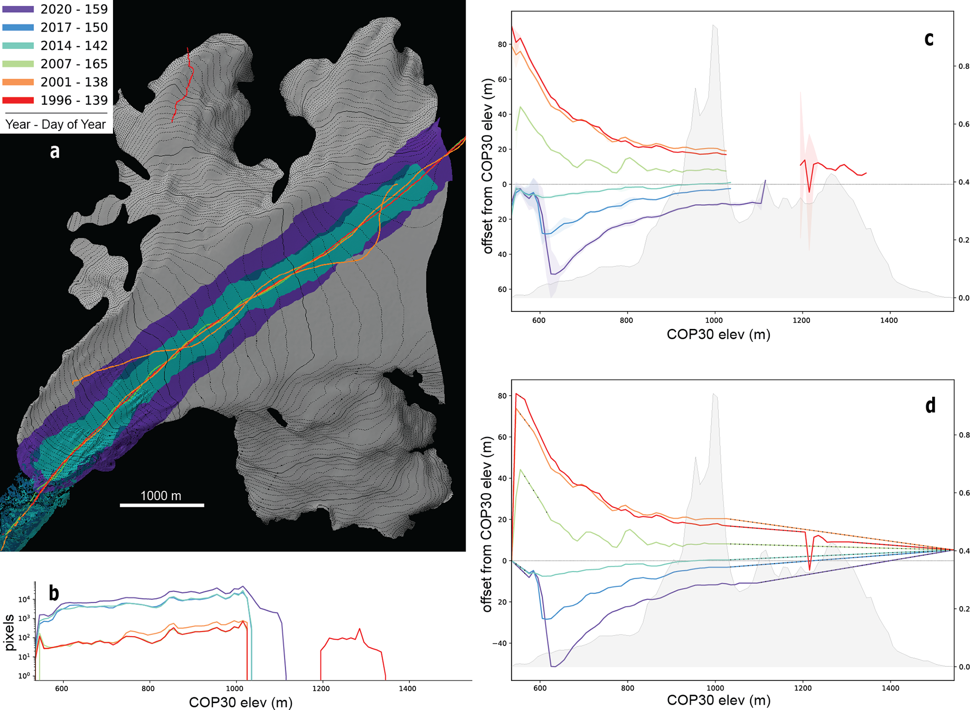
Relative glacier surface elevations at each measurement interval (the offsets from COP30 DEM as described above) can be visually compared as shown in Fig. 2b but require filtering and gap filling for glacier-wide mass-balance calculations. Most outliers in each glacier’s median offsets occur in bins with very few laser measurements, presumably due to off-nadir returns captured from otherwise unmeasured glacier areas during aircraft maneuvering. To filter out these anomalous values, for every laser flight we calculate the frequency distribution of pixel counts per bin and discard measurements from the bottom 10% of the distribution. We then fill gaps in the filtered data with ‘synthetic’ data as described below.
Example of survey/processing workflow. (a) Hillshade of Kachemak Glacier with 10 m contour lines and terminus at lower left. Colored swaths are profiler (narrow) and scanner (wider) survey tracks, identified in the inset legend. (b) Number of 2.5 m pixels surveyed per 10 m elevation bin. Note logarithmic  $y$-axis. (c) Raw offsets of survey elevations from the COP30 DEM, in meters. Shading around lines indicates the binned interquartile range of elevation offsets. (d) Same data after filtering, as described in text. Black dots on lines indicate synthetic data where the offset has been interpolated or extrapolated. Gray histograms in (c) and (d) are the distribution of glacier area by elevation, with the binned areas (in km2) indicated on the secondary
 $y$-axis. Analogous figures for all survey epochs are available in the data repository at Loso and others (Reference Loso, Fahnestock, Larsen and Tober2026).

Figure 2 Long description
Four panels (a through d) detail the data processing workflow on Kachemak Glacier: a) Hillshade map showing narrow profiler and wider scanner airborne survey tracks along the centerline across multiple years; b) Semi-logarithmic plot showing the number of 2.5 m pixels surveyed per 10 m elevation bin; c) Elevation offsets between raw laser survey heights and the COP30 reference DEM across elevation bins, with shaded interquartile ranges and hypsometry histograms; d) Elevation offsets after filtering out the lowest 10% sample bins and applying linear interpolation and high-elevation extrapolation (synthetic data indicated by black dots).
At the glacier terminus, offsets of any unsurveyed bins are linearly extrapolated from the value of the lowest surveyed bin to 0 m offset at the terminus. Gaps between surveyed bins are linearly interpolated from the values of next lowest and highest surveyed bins. Extrapolation to the offset of the highest glacier elevation, where gaps are usually the largest, requires more steps. First, because offsets in the highest measured elevations, even after filtering, are typically quite noisy, we smooth them by replacing the values of the five highest measured bins with their collective median value. Previous investigators would commonly then extrapolate to zero offset at the highest glacier elevation based on the assumption that glacier change is typically minimal near the mountain summits. Offsets of the higher-elevation UAF measurements from the COP30 DEM do not trend towards zero, however. Close inspection of the highest elevation offsets reveals a distinct seasonal pattern to these offsets (Fig. 3), with larger offsets in March measurements and the smallest offsets in August. We attribute these non-zero offsets to two factors: 1) X-band radar penetration depressing evident surface elevations in the highest elevations of the COP30 DEM, and 2) seasonal snowpack variability, typically near a maximum in March and a minimum in August, elevating evident surface elevations in the highest observed terrain. For any given glacier measurement, we therefore fill high-elevation gaps by extrapolating from the highest measured observation to an offset, at the highest glacier elevation, equal to the median offset of the highest surveyed bins from all measurements during that season, as shown in Fig. 3.
Observed offsets of the COP30 DEM from the highest observation on each UAF glacier at each survey epoch, grouped by season of measurement. Surveyed elevations were consistently higher (positive offsets) with a distinct seasonal trend. Boxes bracket the interquartile range (iqr) of each season’s measurements with the notched red line at the median value. Notches show 95% confidence intervals around the median, and whiskers extend above/below the box to the highest/lowest value, respectively, within 1.5iqr of the box. For this analysis,  $n$ = 24 (March), 171 (May) and 100 (August). Outliers are omitted for clarity.

Figure 3 Long description
A seasonal box-and-whisker plot displaying vertical height offsets at the highest observed glacier elevations compared with the COP30 reference DEM. The data are grouped into three distinct seasons: March (24 epochs, median offset of 7.5 m), May (171 epochs, median offset of 4.8 m), and August (100 epochs, median offset of 1.7 m). The consistently positive offsets reveal a seasonal cycle driven by maximum snowpack accumulation in March and summer ablation minima in August.
We used the filtered and gap-filled offsets from each laser flight (Fig. 2d) to calculate glacier-wide mass balances for each glacier. Because of the significant impact of seasonal changes on glacier surface elevations, for each glacier we only compared offsets collected during the same season. This creates more than one mass-balance time series for the 12% of surveyed glaciers which have measured balances in two or more of the three seasons (e.g., May offsets and August offsets). For each glacier, the binned offsets from all same-season measurements were differenced, yielding for each sequential pair of measurements (each ‘survey epoch’) a single median elevation change,  $\Delta z$, for each bin. We multiplied these by the area of each bin to assess volumetric changes. Bin areas were based upon RGI 7.0 outlines and the COP30 DEM hypsometry and hence remained fixed among all laser flights. Volumetric changes were converted to mass using a two-part density assumption following Gardner and others (Reference Gardner2013). Volume changes below the equilibrium line altitude (ELA) were assumed to involve ice with a density of
 $900 \pm 17\,\, \text{kg}\ \text{m}^{-3}$, while changes above the ELA were assumed to include an unknown mixture of snow, firn and ice represented by a more variable density of
 $700 \pm 200\,\, \text{kg}\ \text{m}^{-3}$.
Annual ELAs were modeled over the temporal span of the UAF record through an optimization scheme using a monthly temperature index mass-balance model (Maussion and others, Reference Maussion2019), and the lowest modeled annual ELA for each glacier was used as the breakpoint dividing the accumulation and ablation zones. Our minimum modeled ELAs for the surveyed glaciers are on average 69 m lower than the minimum ELAs observed by Zeller and others (Reference Zeller, McGrath, Sass, Florentine and Downs2025) from 2018 to 2022, as might be expected given that our modeling covered a longer and earlier time period that includes some less negative (or even positive) balance years. The lowest ELA was chosen to maximize the likelihood that ablation zone elevation changes reflected changes in thickness of ice rather than firn.
Binned mass changes were summed and divided by the elapsed decimal years to yield a glacier-wide mass-balance rate  $({\dot{B}})$ for each epoch, for clarity converted from mass to length units (water equivalent) presented as
 $\text{m}\,\, \text{w.e.}\ \text{a}^{-1}$. Because the rate for a given glacier and survey epoch might represent the change over a period of one to several years, statistical summaries of the derived rates were weighted by the length of each epoch. We examined the entire mass-balance dataset for evidence of temporal variability by performing permutation tests (Good, Reference Good2013). We performed weighted polynomial regressions of balance rate against time, where the central date and balance of each survey epoch is a data point, increasing the polynomial degree from zero (constant) to three (cubic). For each regression above degree zero, we first recorded the coefficient
 $ (a_{obs})$ of the highest leading term in the function, then iteratively recalculated the weighted regression after randomly shuffling the dependent variable: balance rates. The distribution of leading term coefficients
 $({a^{*}})$ from 10 000
 $(n)$ random permutations represents the null hypothesis that the leading term describes only random variability, and a
 $p$-value was calculated to describe the likelihood that the actual variability arose by chance, where
 $ p = \frac{ \Sigma{\left( \lvert{a^*}\rvert \,\ge\, \lvert{a_{obs}}\rvert \right) } } {n}$.
Regional mass changes were calculated for all RGI Region 1 glaciers by first using linear regression to calculate an elevation-specific thinning rate for each bin on every UAF glacier with two or more observations. For these regressions, our reference dataset consists of binned offsets (filtered and gap-filled, as before) as a function of time, in most cases limited (because of evidence presented later for an acceleration in mass loss rates) to offsets measured from 2008 onwards. We followed Johnson and others (Reference Johnson, Larsen, Murphy, Arendt and Zirnheld2013) by normalizing the elevation ( $h_{\text{norm}}$) of each bin, where for each glacier
 $h_{\text{norm}} = \frac{{\text{Height above minimum elevation}}}{\text{Total elevation range}}$. Because of our interest in national parks, we used park boundaries as a basis for regionalizing these results. For four park units without any surveyed glaciers, we used the reference data from glaciers in the nearest park unit (Denali data for Gates of the Arctic, Glacier Bay data for Klondike-Gold Rush, Lake Clark data for Katmai and Kenai Fjords for Aniakchak). This reduces our confidence in the mass loss estimates for those parks, but we note that their glacier cover is relatively low. Combined glacier cover in those four units is only 2% of that in all Alaskan parks combined. We performed similar analyses for A) all surveyed glaciers outside park boundaries and B) all surveyed glaciers. For each group of glaciers, we used locally weighted scatterplot smoothing (LOWESS; Cleveland Reference Cleveland1979) with a smoothing parameter (frac) of 0.5 to fit a trendline to the thinning rates as a function of
 $h_{\text{norm}}$. We chose the nonparametric LOWESS technique to avoid imposing a functional form on thinning gradients, which can differ sharply across glacier types and climate regimes. We then applied that regression to the normalized bin elevations of all unmeasured glaciers in a given group, applying the same density assumption described above, to infer overall mass loss rates.
Corroboration and uncertainties
We assessed our results in three different ways: comparison of glacier-wide balances with a previous but methodologically distinct analysis of part of this same dataset, comparison of balances with an analysis using different data and methods, and a numerical assessment of our confidence intervals. Larsen and others (Reference Larsen, Burgess, Arendt, O’Neel, Johnson and Kienholz2015) analyzed an early (1994–2013) subset of the same UAF laser altimetry observations using slightly different methods, filters and assumptions. As a check on our updated methods, we identified glacier epochs that were measured in both their study and ours and compared the derived glacier-wide balance rates with an expectation that the results should be quite similar. We also compared our results with those of Hugonnet and others (Reference Hugonnet2021a), who assessed balances relying primarily on ASTER imagery over the period 2000–19. We aligned the integer years of our measured epochs with those reported as annual per-glacier rates by Hugonnet in dh_01_rgi60_pergla_rates.csv, allowing up to 1 year of deviation but noting that their reported epochs commonly break at the calendar year (1 January) and hence do not precisely match the seasonal timing of our measurements (Hugonnet and others, Reference Hugonnet2021b).
Finally, we calculated mass-balance uncertainties. We base our estimate of variability on the interquartile ranges of the binned offsets between laser measurements and the reference COP30 DEM ( $IQR_{offset}$, shown for example in Fig. 2c). Because each offset is computed as a laser elevation minus the co-located COP30 pixel elevation, large-scale topographic relief within each bin, which both instruments observe, largely cancels in this per-point differencing. So too does any broadly distributed absolute height error in the COP30 DEM. This cancellation is empirically confirmed:
 $IQR_{offset}$ is approximately 4–5 times smaller than either the IQR of the raw laser elevations or the IQR of the raw COP30 elevations within the same bin footprint (median values of
 $\sim$1–2 m for
 $IQR_{offset}$ versus
 $\sim$4–5 m for each raw elevation field). What remains in
 $IQR_{offset}$ reflects three physically meaningful sources of variability: 1) fine-scale surface structures (crevasses, seracs, etc.) resolved by the laser but not by the 30 m COP30 DEM; 2) within-bin spatiotemporal irregularity of melt and accumulation; and 3) instrument noise from both sensors. The first two sources reflect advection and evolution of small-scale surface features that contribute genuine uncertainty in the median offset as an estimate of bin-wide surface change. Laser instrument noise, estimated by previous studies as contributing a net horizontal and vertical positioning error of
 $\pm{0.2} \, \text{m}$ (Johnson and others, Reference Johnson, Larsen, Murphy, Arendt and Zirnheld2013; Larsen and others, Reference Larsen, Burgess, Arendt, O’Neel, Johnson and Kienholz2015), also contributes real uncertainty. COP30 pixel-level noise is the only component of
 $IQR_{offset}$ that is strictly artifactual. We do not have a good means of estimating that pixel-level noise, but because the COP30 has a large 30 m sampling resolution and because it is an edited product that has already been gap-filled with spikes and holes smoothed by interpolation (Marešová and others, Reference Marešová2021), we assume that the noise is small relative to the other sources of variability described above. For that reason, we retain it, making our confidence intervals slightly conservative.
We propagate  $IQR_{offset}$, along with the assumed confidence intervals for our density estimates, into the final glacier-wide balance estimates by first estimating in quadrature the standard deviation (
 $\sigma_{\dot{B}}$) of glacier-wide mass balance for every epoch:
 \begin{equation}
\ \sigma_{\dot{B}} = \sum_{i=1}^{n}\sqrt{\left({\frac{dh}{dt}\cdot A \cdot \sigma_\rho}\right)^2 + \left(\rho \cdot A \cdot \sigma_{\frac{dh}{dt}}\right)^2 }
\end{equation}
where for every bin  $i$ measured on the glacier at two times
 $t$ and
 $t+1$:
 $\frac{dh}{dt}$ is the yearly rate of elevation change in the bin based on the difference between the median offsets at times
 $t$ and
 $t+1$;
 $\sigma_{\frac{dh}{dt}}$ is the uncertainty in the annualized elevation change rate, propagated in quadrature from the
 $IQR_{offset}$ values at the two times as
 $\left(\sqrt{IQR_t^2 + IQR_{t+1}^2}\right) / (1.34 \cdot \Delta t)$;
 $A$ is the area of the bin;
 $\rho$ is the assumed density of the snow/ice/firn gained or lost (
 $700\ \text{kg}\ \text{m}^{-3}$ above the ELA and
 $900$ below); and
 $\sigma_{\rho}$ is the inferred standard deviation of density, calculated from the confidence intervals described earlier as (
 $\pm 200\ \text{kg}\ \text{m}^{-3}$ above the ELA and
 $\pm 17$ below)
 $/$ 1.96. The 95% confidence interval for each mass-balance observation then becomes (
 $\dot{B} \pm 1.96\sigma_{\dot{B}} \, \text{kg}\ \text{a}^{-1}$), which can be converted to
 $\text{m}\ \text{w.e.}$ through division by the glacier area and the density of water. Confidence intervals for each balance observation were propagated into the overall population mean using weighted uncertainty propagation in quadrature, with weights proportional to the duration of each measurement interval.
Results
We begin with an overview of the entire UAF laser altimetry dataset, calculating glacier-wide balance rates for all glaciers, assessing evidence for changes in those rates over time and considering our measurement and extrapolation errors. We also compare those rates with results from two similar studies. Next, we describe spatial patterns of thinning, by elevation, in parks across the study area and extrapolate measured thinning rates to unmeasured glaciers to infer landscape-scale mass loss in each park. We focus that analysis on regional groups defined by National Park boundaries, not in contention that ‘park glaciers’ differ substantively from those outside the parks but rather to emphasize the impacts, within these protected areas, of ongoing glacier change. Finally, we consider temporal changes in extrapolated thinning rates for glaciers throughout the study area.
Glacier-wide balance rates
Glacier-wide balance rates were predominantly negative throughout the measurement period and grew increasingly so over time (Fig. 4). The red lines in Fig. 4a show balance rates calculated for each survey epoch bracketed by two glacier survey flights on the same glacier during the same season. To avoid undue reliance on synthetic (as opposed to measured) data, we exclude ‘incomplete’ surveys from Fig. 4a and from all subsequent analyses, defined here as glacier survey flights that include valid measurements in elevation bins that collectively cover  $ \lt 50\%$ of the glacier area. Figure 4b shows the coverage of all 1349 glacier survey flights, highlighting these 266 (20%) ‘incomplete’ surveys. Balances shown in Fig. 4b reflect variations in survey intensity over time; the yearly number of distinct epochs with calculated mass balances grew to a peak of 257 in 2013 and declined thereafter (Fig. 4c). We note that all results, including data from incomplete surveys, are available in the data repository (Loso and others, Reference Loso, Fahnestock, Larsen and Tober2026).
Glacier-wide mass balances for all surveyed glaciers. (a) Each horizontal red line is a survey epoch that spans between two laser flight survey dates, representing a single glacier’s mass-balance rate, in  $\text{m}\,\, \text{w.e.}\ \text{a}^{-1}$, over that period. Values in red boxes denote magnitude and timing of outlier epochs not shown at this scale. Dashed black line shows statistically significant accelerating thinning trend with quadratic polynomial fit to temporal midpoint of all plotted balances; solid black lines are pre- and post-2008 mean balances.
 $X$-axis tick marks and centers of histogram bars align with the mid-point of a calendar year. (b) Inset shows the hypsometric coverage of all laser survey flights. 266 ‘incomplete’ surveys covered less than 50% of a glacier’s hypsometry (tan bars) and were not used for panels a or c. (c) Counts of glacier epochs with calculated balance results, by year.

Figure 4 Long description
Three panels summarize glacier-wide balance rates: a) Timeline chart from 1994 to 2021 where each horizontal red line represents a single glacier epoch mass balance rate (in meters water equivalent per year). A dashed curve shows a statistically significant quadratic fit indicating accelerating mass loss, with mean rates shifting from -0.83 m w.e. per year before 2008 to -1.16 m w.e. per year thereafter; b) Inset histogram showing the distribution of hypsometric coverage across 1,349 survey flights, highlighting 266 incomplete flights covering under 50% of glacier area; c) Bar chart showing the annual number of active survey epochs with calculated mass balances, peaking at 257 in 2013.
The median 95% confidence interval (CI) for individual epoch balances (CIs are tabulated with balance rates in Table S1 but for clarity not shown in Fig. 4a) was  $\pm{1.49} \,\, \text{m}\,\, \text{w.e.}\ \text{a}^{-1}$. CIs were influenced most strongly by variability of measured surface elevations. Density variability (the
 $\sigma_{\rho}$ term in Eqn (1)) was on average only 46% as large as the
 $\sigma_{\frac{dh}{dt}}$ term, and was typically even less important in epochs with large CIs. Anomalous balances (very high or low) and larger CIs were strongly associated with shorter epochs: for example, 8 of 10 epochs with the largest CIs were from single-year epochs. Shorter epochs have a higher signal-to-noise ratio and must therefore be treated with more skepticism than longer balance epochs, but most nonetheless appear to reliably document annual-scale glacier change. For example, many UAF glaciers were surveyed in 2011 and again in 2012, recording over that short interval relatively high balance rates (37 of 39 glaciers had positive balances, median
 $= 0.83 \,\, \text{m}\,\, \text{w.e.}\ \text{a}^{-1}$) that appear anomalous in Fig. 4 but are corroborated by findings of positive balances on several Alaskan glaciers with field-based glaciological mass-balance programs (Sass and others, Reference Sass, Loso, Geck, Thoms and McGrath2017; O’Neel and others, Reference O’Neel2019).
To determine whether observed trends in Fig. 4 reflect true acceleration of thinning rather than noise among survey intervals, we tested the temporal structure of the record statistically. Permutation testing provided strong evidence to reject the null hypothesis that all temporal variability in epoch balances was random over the UAF laser altimetry campaign. A quadratic polynomial with balance as the  $y$-variable and years as the
 $x$-variable (
 $y = -0.0038x^2 + 15.319x - {153 44.27}$, Fig. 4a) fit the balance data significantly better (
 $p=0.023$) than a constant or a linear regression. Higher degree polynomials did not significantly improve the fit. The quadratic fit shows typical mass loss remained around
 $-$1.0
 $\text{m}\,\, \text{w.e.}\ \text{a}^{-1}$ until a little before 2010, when the balance trend becomes increasingly negative despite positive balance years on some glaciers (especially in winter 2011–12). Collectively, these measurements document a strong and statistically significant acceleration of the thinning rate for all UAF glaciers in RGI Region 1 (Alaska and neighboring Canada).
Balances shown in Fig. 4 and discussed above treat each glacier/epoch as a single observation. Because most glaciers were surveyed across multiple epochs, and also because some glaciers have independent overlapping epochs measured in different seasons, we calculated a single average balance for each glacier. The first step was to calculate the average balance of all epochs for a given glacier in a given season, weighting observations by epoch length. Then, for each glacier with an independent time series of survey flights from more than one season, we averaged the derived balance rates from all seasons, again weighting by epoch length. From the resulting list of each glacier’s overall balance rate (tabulated in Table S1), we then calculate for the entire dataset a single average and 95% confidence interval of  $-1.06 \pm{0.07} \,\, \text{m}\,\, \text{w.e.}\ \text{a}^{-1}$. We assessed the sensitivity of our results to the piecewise density assumption by re-calculating balances using a glacier-wide bulk density of
 $850 \pm 60\,\, \text{kg}\ \text{m}^{-3}$ (Huss, Reference Huss2013). Averaged again across all glaciers and epochs, the bulk density assumption yielded a slightly more negative glacier-wide balance with a comparable confidence interval (
 $-1.18 \pm{0.08} \,\, \text{m}\,\, \text{w.e.}\ \text{a}^{-1}$).
In light of the evidence for accelerated thinning described above, and because an average balance calculated for the entire dataset is biased towards the recent period by the larger number of surveyed glaciers, we used the same techniques to calculate average rates for an early period that includes all complete or partial epochs before 2008 ( $-0.83 \pm{0.13} \,\, \text{m}\,\, \text{w.e.}\ \text{a}^{-1}$) and a late period after 2008 (
 $-1.16 \pm{0.08} \,\, \text{m}\,\, \text{w.e.}\ \text{a}^{-1}$). Note that these statistics, plotted in Fig. 4, treat each glacier equally and are not weighted by glacier area.
We confirmed that these mass-balance rates are very similar to those reported, using the same laser measurements for the same glaciers and epochs but using different analytical techniques, in Table S1 of Larsen and others (Reference Larsen, Burgess, Arendt, O’Neel, Johnson and Kienholz2015). Our mean glacier-wide balance rate for just the epochs reported by both papers is very slightly less negative than that of the 2015 study with low variability ( $\overline{\text{diff}}$ = 0.05,
 $\sigma = 0.18 \,\,\text{m}\,\,\text{w.e.}\ \text{a}^{-1}$, Fig. 5a). We attribute those small differences mainly to the double-differencing technique that allowed us to use more of the collected survey data; Larsen and others (Reference Larsen, Burgess, Arendt, O’Neel, Johnson and Kienholz2015) discarded any survey data without a direct spatial overlap of other measurements. We also compared the average glacier-wide mass-balance rate for every surveyed glacier, over all available and broadly coincident epochs, with rates reported in Hugonnet and others (Reference Hugonnet2021b). The glacier-by-glacier differences in Fig. 5b show that the UAF balance rates are overall less negative than those reported by Hugonnet (
 $\overline{\text{diff}}$ = 0.10 ,
 $\sigma = 1.45 \,\,\text{m}\,\,\text{w.e.}\ \text{a}^{-1}$, Fig. 5b). The differences are largest for very short epochs, however, and comparing only epochs 2 years or longer, the two groups are even closer, with UAF rates very slightly more negative than Hugonnet’s (
 $\overline{\text{diff}}$ = -0.03 ,
 $\sigma = 0.73 \,\,\text{m}\,\,\text{w.e.}\ \text{a}^{-1}$).
Distribution of differences between glacier-wide mass-balance rates ( $\dot{B}$) estimated by this and other studies. Each epoch counted in either histogram represents one measured interval on a single glacier. Vertical solid line highlights zero difference in both panels; dashed line is mean difference
 $(\overline{\text{diff}})$. Note varying scales. (a) UAF laser altimetry intervals from this study compared to identical intervals reported by Larsen and others (Reference Larsen, Burgess, Arendt, O’Neel, Johnson and Kienholz2015) using the same data but different methods. Our new balances overall were very slightly less negative. (b) Mass balances from this study compared with Hugonnet and others (Reference Hugonnet2021a) estimates for comparable years. Short 1-year epochs (‘
 $ \lt 1.5\,\mathrm{a}$’) are distinguished from multi-year epochs. UAF glacier balances from this study were overall less negative than Hugonnet’s.

Figure 5 Long description
Two comparison histograms: a) Distribution of mass balance differences for identical intervals between this study and Larsen et al. (2015) using the same lidar data, showing a tight distribution centered near zero (mean difference = +0.05 m w.e. per year); b) Distribution of balance differences compared to satellite-derived ASTER estimates from Hugonnet et al. (2021a), distinguishing short epochs (<1.5 years) from multi-year epochs (≥1.5 years), showing close agreement for multi-year intervals (mean difference = -0.03 m w.e. per year).
Thinning rates
Figure 6 maps the patterns of mostly negative elevation changes (thinning) for all UAF glaciers in the five national park units for which we have measurements. In all cases, the plotted thinning rates ( $dh/dt$) are averaged over the full span of all UAF measurements for that glacier, excluding incomplete measurements with
 $ \lt 50\%$ coverage as described earlier. Plotted rates are derived from filtered and gap-filled offsets as shown, for example, in Fig. 2d, and for display purposes have been rastered across the full width of every bin, though measurements were typically near the centerline as shown in Fig. 2a. In all parks, thinning rates are generally low (0.0 to
 $-$0.9
 $\text{m}\,\, \text{a}^{-1}$, yellow hues) in most glacier accumulation areas, trending towards more negative rates (
 $-$1.0 to
 $-$3.9
 $\text{m}\,\, \text{a}^{-1}$, tan hues) at glacier termini. Rates more negative than
 $-$5.0
 $\text{m}\,\, \text{a}^{-1}$ (red hues) are less common but most conspicuously evident at lower elevations of Tuxedni Glacier (Lake Clark); Steller, Agassiz and Malaspina Glaciers (Wrangell-St. Elias); and La Perouse, Carroll, Casement and Grand Plateau Glaciers (Glacier Bay). Evidence of modest localized glacier thickening (positive rates) is visible in many glacier accumulation zones and near the terminus of tidewater Hubbard Glacier, and more significant thickening is noticeable on portions of surging glaciers like Muldrow Glacier (Denali) and Klutlan and Logan Glaciers (Wrangell-St. Elias).
Annual thinning rates ( $dh/dt$,
 $\text{m}\,\, \text{a}^{-1}$) averaged over all epochs of surveyed glaciers. Panels a through f focus attention on NPS unit glaciers at 1:1 900 000 scale, as shown in the inset map at upper right: (a) Denali, (b) Lake Clark, (c) southern Wrangell-St. Elias, (d) northern Wrangell-St. Elias, (e) Glacier Bay and (f) Kenai Fjords. Numerals identify glaciers discussed in text: 1) Tuxedni, 2) Steller, 3) Agassiz, 4) Malaspina, 5) La Perouse, 6) Carroll, 7) Casement, 8) Grand Plateau, 9) Hubbard, 10) Muldrow, 11) Klutlan and 12) Logan.

Figure 6 Long description
A six-panel regional map collection (panels a through f) depicting average long-term surface thinning rates (dh/dt) across individual glaciers in key National Park units: a) Denali, b) Lake Clark, c) southern Wrangell-St. Elias, d) northern Wrangell-St. Elias, e) Glacier Bay, and f) Kenai Fjords. Glacier colors represent thinning rates: yellow and tan indicate moderate thinning (0 to -3 m per year), deep orange and red indicate rapid thinning (-4 to <-8 m per year) concentrated at lower elevations and retreating termini, and blue denotes localized thickening or surging activity.
Overall mass loss
Histograms summarizing measured elevation change rates by normalized elevation bin in each park unit since 2008 and in a sixth group of surveyed glaciers outside all park boundaries are shown in Fig. 7. Trendlines fit to each full dataset are shown in white and allow us to extrapolate the reference data trends to unsurveyed glaciers. The histograms display some substantial outliers, and we attribute this noise mainly to the presence within our reference data of tidewater, lake-terminating and surging glaciers whose dynamics are triggered by more than just regional climate. Rather than manually and somewhat subjectively remove such glaciers from the reference datasets, or stratify the glaciers by type as was done by Larsen and others (Reference Larsen, Burgess, Arendt, O’Neel, Johnson and Kienholz2015), we experimented with an automated approach to identifying and filtering out the impacts of transient glacier dynamics. For each glacier, we calculated in each elevation bin the standard deviation of a regression line fit to all observed thinning rates (except in cases where there were fewer than three observation intervals). We then created a filtered version of the reference dataset which excludes thinning rates from each glacier’s elevation bins where standard deviation exceeded 0.5  $\text{m}\,\, \text{a}^{-1}$. Trendlines fit to this filtered dataset are shown in red in Fig. 7.
Histograms summarizing observed thinning rates from 2008 to 2022 as a function of normalized glacier elevation. Summarized glaciers are grouped by park, with an additional grouping for surveyed glaciers completely outside all park boundaries (‘NONE’). See Table 2 caption for full park names. Histograms display data in 40 groups on each axis, and colorbar summarizes number of individual observations (‘Count’) within that group. Note colorbar scales vary. White trendline is lowess fit to all observations, while red line is lowess fit using filtered observations only: bins with consistent thinning rates over time as described in text.

Figure 7 Long description
A grid of six two-dimensional histograms displaying data counts of observed annual thinning rates (2008-2022) plotted against normalized glacier elevation (from 0.0 at the terminus to 1.0 at the head). Panels show results for glaciers outside parks (NONE) and five individual park units (WRST, DENA, GLBA, LACL, KEFJ). White curves show LOWESS fits to all observations, while red curves show LOWESS fits to dynamic-filtered data, consistently demonstrating strong elevation gradients with rapid thinning near termini that approaches zero near upper accumulation zones.
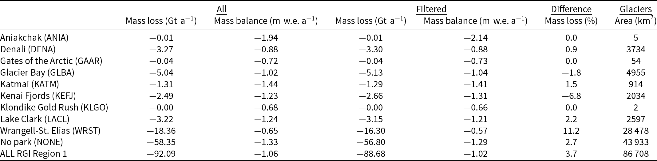
We applied these thinning rate trends to unmeasured glaciers to estimate total yearly mass loss from each park from 2008 to 2022 (Table 2). We emphasize that the generally more rapid rates of recent thinning used in this analysis are distinct from the overall 1993–2022 rates shown in Fig. 6. The filtering technique described above had minimal impact on the results, leading to an overall difference in summed regionwide mass loss (compared with unfiltered data) of only 3.7%, with even smaller differences in many individual parks. We show both versions in Table 2 but choose in the following narrative to focus on results using the more complete unfiltered (‘ALL UAF’) reference dataset.
Inferred rates of glacier change between 2008 and 2022 for RGI Region 1 glaciers, grouped by presence in or outside of glacierized National Park units. Note four-letter abbreviations of park names in parentheses. Mass loss is a cumulative sum across all glaciers; mass balance is the glacier-wide value averaged across all glaciers. Values grouped under ‘All’ are extrapolated from all valid data. Values under ‘Filtered’ were extrapolated from a limited dataset, as described in text. ‘Difference’ highlights the percentage by which the filtered mass change is greater or less than the change using all data.

Table 2 Long description
A structured data table summarizing extrapolated glacier changes from 2008 to 2022 across nine National Park units (Aniakchak, Denali, Gates of the Arctic, Glacier Bay, Katmai, Kenai Fjords, Klondike Gold Rush, Lake Clark, Wrangell-St. Elias), non-park glaciers (NONE), and the entire RGI Region 1. Columns provide total mass loss (Gigatons per year) and area-averaged mass balance (meters water equivalent per year) for both all-data and filtered-data extrapolations, as well as percentage differences and glacier areas. Cumulative park glacier mass loss is estimated at 33.74 Gt per year out of a regional total of 92.09 Gt per year.
Reported mass losses scale generally with the amount of glacier cover in a park, so that Wrangell-St. Elias National Park and Preserve has the largest overall mass loss of any park ( $-$18.36
 $\text{Gt a}^{-1}$; more than all the other parks combined). Collectively, we estimate that NPS glaciers lost 33.74
 $\text{Gt a}^{-1}$ of ice between 2008 and 2022. By extending our analysis to the entirety of RGI Region 1, we infer that this contribution of NPS glaciers constitutes 1/3 of the estimated rate of mass loss from all of Alaska and neighboring Canada:
 $-$92.09
 $\text{Gt a}^{-1}$ (Table 2). That statewide number depends, however, upon an estimate of mass loss in all the non-park glaciers. That group (‘NONE’ in Fig. 7 and Table 2) is based upon a diverse reference dataset: non-park glaciers of all sizes and types from around the state. For the earlier 1993–2008 interval (not shown in Fig. 7 or Table 2), we estimate a mass loss of
 $-$69.83
 $\text{Gt a}^{-1}$ for RGI Region 1, suggesting a 32% increase in annualized mass loss from the 1993–2008 to the 2008–22 interval.
Discussion
The processed results from UAF laser altimetry surveys summarize three decades of significant change in glaciers that include over half of the total glacierized terrain in Alaska and adjacent Canada. Given this vast and sparsely developed landscape with more than 27 000 individual glaciers, articulating the specific local consequences of these changes is inherently challenging. Consequently, large-scale studies tend to focus on regional and global outcomes. Our experience in the Alaskan National Parks, where glaciers are both dominant features and primary attractions, drives us to emphasize the local impacts of glacier change. After discussing regional trends, we then highlight specific examples of how accelerating mass loss directly affects park landscapes and the people who visit, manage and inhabit these areas. Those examples rely upon only a few of the detailed surface evolution histories contained in this dataset, so we emphasize here that the geographically and statistically granular offset histories of all 205 UAF glaciers are available in a public data repository (Loso and others, Reference Loso, Fahnestock, Larsen and Tober2026). Those complete results, based upon the underlying NSIDC archive (Larsen, Reference Larsen2010), constitute a primary contribution of this work.
Regional trends
The altimetry-based histories provided here provide exceptional accuracy and spatial resolution but collectively omit a significant amount of the glacier cover in RGI Region 1, including A) unmeasured portions of surveyed glaciers (lateral margins and steep terrain), and B) the 27 304 unsurveyed glaciers that represent almost 44% of the ice by area in Alaska and adjacent Canada. With respect to the first issue, we are confident that our local extrapolations of binned  $\frac{dh}{dt}$ provide a robust estimate of unmeasured changes on the margins of individual glaciers. This assumption was tested on a subset of the UAF glacier data by Johnson and others (Reference Johnson, Larsen, Murphy, Arendt and Zirnheld2013), who found differences of
 $ \lt 6\%$ when comparing glacier-wide mass balances from differencing of full DEMs to those derived from longitudinal altimetry profiles. We note that this is similar in magnitude to the difference we found between our extrapolations of glacier-wide mass balance and those of Larsen and others (Reference Larsen, Burgess, Arendt, O’Neel, Johnson and Kienholz2015) using the same data but different methods (Fig. 5). Johnson and others (Reference Johnson, Larsen, Murphy, Arendt and Zirnheld2013) also concluded that their use of fixed glacier boundaries (as in our analysis) had minimal effect on derived balances. Fixed outlines might have caused us to slightly underestimate volume changes at the extended termini of some glaciers measured before the RGI outlines were drawn, while having no significant impact on volume changes of retracted termini later in the record. Our conclusions are robust to this effect because the glacier-wide balances used for this analysis require division of the volume change by glacier area, which in the latter part of the survey period is often overestimated for these retreating glaciers, leading to a systematic (and conservative with respect to our assertion of accelerating mass loss) bias towards artificially low balance estimates towards the end of the period. Glacier-wide laser measurements and a catalog of evolving glacier outlines would improve the accuracy of our mass-balance estimates on surveyed glaciers, but these factors are all small when compared with the reported confidence intervals for each glacier (Table S1), which are driven by within-bin variability of measured surface elevations. We therefore begin with a summary of regional trends based only on these well-constrained results from UAF-surveyed glaciers before turning our attention to the second issue–inference of trends on unsurveyed glaciers.
The UAF laser altimetry record provides strong direct evidence for accelerating mass loss throughout the region between 1994 and 2021. The mass balances shown in Fig. 4 are predominantly negative throughout the period, with some positive balances in the late 1990s and in 2012, and the overall balance rate is  $-1.06 \,\, \text{m}\,\, \text{w.e.}\ \text{a}^{-1}$. Permutation testing confirmed the statistical significance of a trend towards increased mass loss at the end of the period, with survey-wide balances decreasing from
 $-$0.83
 $\text{m}\,\, \text{w.e.}\ \text{a}^{-1}$ before 2008 to
 $-$1.16 after. We acknowledge the importance of choosing carefully how to summarize the full dataset. One could, for example, divide the ‘early’ and ‘late’ periods on a different year than 2008, or filter the data to exclude certain glaciers using different criteria. In part to facilitate such alternate analyses, the entire dataset is available in an online repository (Loso and others, Reference Loso, Fahnestock, Larsen and Tober2026), but we contend that for surveyed UAF glaciers the principal finding of widespread negative mass balances growing more so over time is broadly insensitive to such choices.
Extrapolation of thinning rates to unmeasured glaciers allows us to estimate total mass losses within the National Parks. The largest and most glacierized park (Wrangell-St. Elias) had the highest mass loss, but area-averaged rates of mass loss (mass balances), whether filtered or not, are smallest in Wrangell-St. Elias. We attribute that finding to the strong influence, in this analysis, of the very large Hubbard Glacier. Hubbard, like many tidewater glaciers, often behaves out of synchrony with regional climate-driven trends (Post and others, Reference Post, O’Neel, Motyka and Streveler2011) and over the period of our observations had the third highest mass balance ( $-$0.07
 $\text{m}\,\, \text{w.e.}\ \text{a}^{-1}$). Because the histograms in Fig. 7 are pixel-based, average measured thinning rates in this analysis are weighted toward larger glaciers implicitly; this contrasts with the prior analysis of balance rates shown in Fig. 4, which treated each glacier’s mass balance with equal weight. The relatively low thinning rates measured on Hubbard Glacier (the third largest surveyed glacier) therefore have an outsize impact on the trendlines used to estimate thinning on other unmeasured glaciers in Wrangell-St. Elias, leading us to infer slower thinning rates on the many land-terminating glaciers in that park. This highlights the potential advantages of climatic and/or dynamic stratification of glaciers, as was done, for example, by Larsen and others (Reference Larsen, Burgess, Arendt, O’Neel, Johnson and Kienholz2015). Led by our interest in National Parks, we chose to stratify instead by national park boundaries (Table 2).
We examine the validity of this approach to estimating balances on unmeasured glaciers, both in the parks and out, by running an analogous analysis on the 2000–19 mass balances measured in a recent photogrammetric analysis of more spatially complete ASTER satellite imagery (Hugonnet and others, Reference Hugonnet2021a). Using the same subset of Alaskan glaciers measured in the present study, we developed elevation-specific thinning rates using the Hugonnet ‘observations’ (derived from DEM differencing) and then extrapolating those regressions to the glaciers we did not survey, stratified by park (including all the glaciers outside the parks, denoted by ‘NONE’). We then compare the Hugonnet observations (complete in each region) with the balances estimated from their data in exactly the same way as completed in this study (Fig. 8). The results of that analysis provide insight into the ability of the surveyed glaciers to faithfully predict balances of the larger population within the sampling units (parks) we selected. In the Hugonnet dataset, park-wide balances for Aniakchak (ANIA) and Katmai (KATM) are poorly predicted by our extrapolation technique. This is perhaps expected, given that there were no glaciers surveyed in those parks and the balances are extrapolated from distant areas. Surprisingly, the same situation results in better predictions for Klondike-Gold Rush (KLGO) and Gates of the Arctic (GAAR). All of those park units, in any case, have very small glacier coverage relative to the state as a whole. It is encouraging that balances on the ‘non-park’ glaciers (NONE), which is a large and geographically diverse group, are predicted within 7% of observed values, and that extrapolated balances in the entire statewide group (ALL) are similarly only 10% more negative than observations. Of the heavily glacierized and well-surveyed parks, Glacier Bay (GLBA) stands out as an anomaly, with the extrapolated balance 23% less negative than Hugonnet’s observations. We attribute that to the large number and areal coverage of tidewater glaciers in that park, which as noted above behave in unique and sometimes divergent ways to regional climate forcings (Post and others, Reference Post, O’Neel, Motyka and Streveler2011). A regression of extrapolated regional balances against observed balances, weighted by the proportion of surveyed glaciers, is negatively impacted by that Glacier Bay estimate and closely tracks the 1:1 line only in a separate regression from which that park is excluded.
Observed and extrapolated glacier-wide balances derived from the 2000 to 2019 results of Hugonnet and others (Reference Hugonnet2021a) using the same extrapolation scheme applied to UAF thinning rates in this paper. Glaciers are grouped by park, with an additional grouping for surveyed glaciers completely outside all park boundaries (‘NONE’). See Table 2 caption for full park names. ‘ALL’ (star) includes all RGI Region 1 glaciers from the other groups and is not included in regressions. Regression line against all groups (dark blue) and against all groups except GLBA (cyan) is weighted by portion of the glacier area that was actually observed in a given group, denoted by colorbar. Dashed line is 1:1.

Figure 8 Long description
A validation scatter plot comparing observed regional mass balances directly against extrapolated estimates derived from satellite-borne ASTER observations (2000-2019). Individual park units and the non-park group are plotted as circles color-coded by the percentage of glacier area surveyed. Regressions show good overall alignment with the 1:1 line for well-sampled parks like Wrangell-St. Elias (WRST) and Denali (DENA), with larger deviations in poorly sampled or tidewater-dominated regions like Glacier Bay (GLBA).
Our own analysis of extrapolated glacier changes estimates that glaciers in Alaska’s nine glacierized National Parks collectively lost 33.74  $\text{Gt a}^{-1}$ of ice from 2008 to 2022 (tabulated by park in Table 2), enough to fill Arizona’s Lake Mead each year to full capacity (Tighi and Callejo, Reference Tighi and Callejo2009). By calculating total mass loss in a tenth area—the ‘non-park’ glaciers—we estimate a complete RGI Region 1 mass loss of
 $-$92.09
 $\text{Gt a}^{-1}$ (all data) or
 $-$88.68
 $\text{Gt a}^{-1}$ (filtered data; Table 2). Our estimate of 92.09
 $\text{Gt a}^{-1}$ translates to an average annual contribution to sea level rise, by glaciers of Alaska and adjacent Canada, of 0.26
 $\text{mm a}^{-1}$ from 2008 to 2022. We lack a rigorous quantitative basis for estimating the uncertainty of our extrapolated mass loss estimates, but conclude from the prior analysis (Fig. 8) that the regional extrapolation scheme we have utilized, while imperfect, generally predicts regional glacier balances within roughly
 $\pm 10$%, but with the potential for more substantial uncertainty in areas with A) tidewater glaciers and/or B) poor survey coverage. We are also encouraged by the close match between our statewide results and the ultimate conclusions of Hugonnet and others (Reference Hugonnet2021a). Using their own observations (distinct from our analysis above), Hugonnet estimated a statewide mass loss of
 $-$87.2
 $\text{Gt a}^{-1}$ during the most recent epoch in their study, from 2015 to 2019. The accuracy and granular detail of our UAF surveys are consistent with, and complement, such space-borne datasets and will continue to be useful for validating their results (The GlaMBIE Team, 2025). Taken together, these patterns demonstrate that accelerating mass loss is not only a regional climate signal but already presents landscape-scale management issues in the National Park system.
Local impacts of glacier thinning
Recent studies have documented some management-relevant implications of glacier changes in Alaskan parks, including glacier collapses (Jacquemart and others, Reference Jacquemart2020), the potential abandonment of culturally important river outlets (Loso and others, Reference Loso2021) and the effects of deglaciation on wildlife (Sytsma and others, Reference Sytsma, Lewis, Bakker and Prugh2023). Anecdotal observations of glacier change reveal many other potentially important impacts on parks, but managers typically require solid scientific evidence to justify their actions—evidence that is frequently constrained by the expense and staff time needed for conducting and disseminating research. Here, we take the opportunity to illustrate, through case studies of one glacier from each park featured in these surveys, some landscape-scale impacts of the glacier thinning revealed by our work. The glacier examples below were selected not because their thinning rates or ice dynamics are anomalous, but rather because they occur in locations that make them especially relevant to park users and managers. Figure 9 indicates their locations alongside the measured and in some cases extrapolated thinning results from this study.
Measured offset histories (left) and mapped thinning rates (right) depict recent changes on five management-relevant glaciers in Alaskan National Parks. Red arrows indicate elevations (left) and corresponding map locations (right) for management issues described in the text: (a) Exit Glacier in Kenai Fjords National Park, (b) Kennicott Glacier in Wrangell-St. Elias National Park and Preserve, (c) Tanaina Glacier in Lake Clark National Park and Preserve, (d) Kahiltna Glacier in Denali National Park and Preserve and (e) Margerie Glacier in Glacier Bay National Park and Preserve. Inset map in the upper right shows thinning rate map locations (red boxes) and National Park boundaries (green polygons).

Figure 9 Long description
Five pairs of plots and maps (panels a through e) illustrate glacier change and associated management issues: a) Exit Glacier (Kenai Fjords), showing up to 5 m per year terminus thinning affecting visitor trails and access roads; b) Kennicott Glacier (Wrangell-St. Elias), showing thinning near historic sites, trailheads, and glacial outburst flood areas; c) Tanaina Glacier (Lake Clark), showing rapid terminus retreat altering drainage into salmon rivers; d) Kahiltna Glacier (Denali), showing thinning near the West Buttress climbing route (Windy Corner) and runway crevasse hazards; e) Margerie Glacier (Glacier Bay), showing terminus thinning threatening cruise ship viewing and harbor seal habitat.
Exit Glacier in Kenai Fjords National Park, accessible within three hours of Anchorage International Airport, receives over 100 000 visitors per year (Kurtz and Baker Reference Kurtz and Baker2016; Fig. 9a). Rapid thinning—up to 5.0  $\text{m}\,\, \text{a}^{-1}$ at elevations around 200 m—has led to significant terminus retreat with notable consequences. Vegetation succession has obscured views of the glacier from a popular viewing platform. A well-used ‘Glacier Overlook Loop Trail’ that used to provide direct access to the ice is now blocked by rocky cliffs, limiting both the accessibility and visibility of the glacier with negative impacts on visitor satisfaction (Kurtz and Baker, Reference Kurtz and Baker2016). Additionally, changes in downstream Exit Creek have repeatedly overrun and damaged the paved access road (Curran and others, Reference Curran, Loso and Williams2017). Each of these changes restricts visitor access to the glacier and necessitates costly repairs for NPS.
Kennicott Glacier, located adjacent to the Kennecott Mines National Historic Landmark in Wrangell-St. Elias National Park and Preserve, is possibly the most pedestrian-accessible large glacier in the state (Fig. 9b). However, it is experiencing various impacts. Thinning rates of about 1.2  $\text{m}\,\, \text{a}^{-1}$ at 930 m are increasing meltwater-driven runoff and, more importantly, the dynamics of an annual glacier-lake outburst flood, threatening two bridges that provide the only overland access to the towns of McCarthy and Kennicott (Rickman and Rosenkrans, Reference Rickman and Rosenkrans1997). Furthermore, a thinning rate of roughly 1.5
 $\text{m}\,\, \text{a}^{-1}$ at the debris-covered terminus (475 m) is facilitating the growth of a proglacial lake, impacting downstream flood regimes while offering new recreational opportunities for visitors (Wells and others, Reference Wells2025). Lastly, NPS trail crews have had to continuously extend built access to the Root Glacier tributary at 690 m as the ice surface deflates at up to 2.0
 $\text{m}\,\, \text{a}^{-1}$.
Lake Clark National Park and Preserve, remote and accessible primarily by bush planes from Anchorage, presents a unique view of ecological shifts at Tanaina Glacier (Fig. 9c). At elevations around 350–400 m, the glacier terminus is thinning at rates of up to 5.0  $\text{m}\,\, \text{a}^{-1}$. While most visitors cannot access this area, they witness a rapidly transforming landscape from the air. Previously, Tanaina Glacier’s runoff flowed west into Summit Lake and subsequently into Lake Clark via the Tlikakila River, a crucial salmon habitat (Young, Reference Young2005). Now, much of that runoff is diverted into the North Fork Big River, altering the discharge and turbidity of the Tlikakila River. This shift raises concerns about the uncertainty of its impacts on salmon and the broader ecosystem.
Denali National Park and Preserve’s Mount McKinley attracts over 1000 mountaineers annually, primarily via the Kahiltna Glacier (Fig. 9d). High on the glacier, thinning rates of less than 1.0  $\text{m}\,\, \text{a}^{-1}$ are destabilizing exposed rocks above ‘Windy Corner’, a bottleneck in the West Buttress climbing route, increasing (along with possible thawing of alpine permafrost) the risk of rockfall for climbers. Further down-glacier, the Southeast Fork of Kahiltna Glacier serves as a busy airstrip for ski-equipped aircraft during the April to July climbing season. However, thinning (1.0
 $\text{m}\,\, \text{a}^{-1}$) and accelerated snowmelt now often render the airstrip unusable in the later climbing season (due to exposed crevasses), compelling pilots to land further up-glacier in areas that remain crevasse-free longer but are threatened by serac falls from Mount Hunter.
Margerie Glacier in Glacier Bay National Park and Preserve is one of the last destinations where cruise ship passengers can witness calving tidewater glaciers up close (Fig. 9e). With thinning rates up to 6.5  $\text{m}\,\, \text{a}^{-1}$, the terminus may soon become grounded. While other tidewater glaciers remain in coastal Alaska, few suitable viewing options exist in the park, posing challenges to its legislative purpose of providing tidewater glacier experiences (Gende and others, Reference Gende, Womble and Bliss2025). Moreover, icebergs calved from glaciers like Margerie and especially nearby Johns Hopkins provide critical habitat for harbor seals, which might suffer significant local population declines where calved icebergs disappear (Womble and others, Reference Womble2021). The park currently restricts cruise ship entrance to Johns Hopkins Glacier during seal pupping time; if Margerie Glacier grounds and ceases to calve, there will be additional pressure to allow vessels close to Johns Hopkins. Park managers will face the challenge of protecting seal habitat while still allowing visitors the opportunity to experience a calving tidewater glacier.
Conclusions
Our synthesis of glacier surface elevations measured in 1349 glacier surveys flown during nearly three decades of airborne laser altimetry provides clear and statistically robust evidence that mass loss from the glaciers of Alaska and adjacent Canada (RGI Region 1) has accelerated markedly since the late 1990s, including from the largest and most visited glaciers in the National Parks. Mean balance rates went from  $-0.83 \pm{0.13} \,\, \text{m}\,\, \text{w.e.}\ \text{a}^{-1}$ before 2008 to
 $-1.16 \pm{0.08} \,\, \text{m}\,\, \text{w.e.}\ \text{a}^{-1}$ thereafter. Our results are consistent with other regional studies that document rapid glacier shrinkage in response to documented climatic changes. These changes have global and regional consequences, but we highlight with several examples the particular glacier-scale importance of ice loss in National Parks: rapid thinning is reshaping landscapes that visitors access, that infrastructure depends upon and that ecosystems are structured around. The NPS has little ability to manage the ultimate climatic cause of these changes, but with a detailed awareness of this trajectory it can mitigate or adapt to the most pressing consequences. Because this work homogenizes and reprocesses the complete UAF laser altimetry record into a consistent, gap-filled and easily queried archive, it creates a lasting public dataset that can support local hazard assessment, park planning, ecosystem research, analysis of seasonal trends and future validation of satellite-based mass-balance products.
Supplementary material
The supplementary material for this article can be found at https://doi.org/10.1017/jog.2026.10187.
Data availability statement
The data and figures for each glacier survey and relevant Python scripts can be found at Loso and others (Reference Loso, Fahnestock, Larsen and Tober2026).
Acknowledgements
Both Keith Echelmeyer and Will Harrison are remembered for originating the laser survey program summarized here. Thanks to Paul Claus, Steve Davidson and Doug Keller (among others) for their flight support, and to collaborators Michael Christoffersen, Jack Holt, Martin Truffer, Anthony Arendt, Sandy Lee Zernheld, Austin Johnson and David Rounce for scientific contributions. The National Park Service Inventory and Monitoring Program contributed to the analysis of these data. Much of the data used in this project was acquired by NASA’s Operation IceBridge, with additional support from NOAA and the National Science Foundation.






 Open access

