NOMENCLATURE
- F max
Maximum packet length in an AFDX network
- C i
Maximum transmission time of a packet generated by flow v i
- T i
Minimum time interval of two consecutive packets generated by flow v i
 ${{\mathscr{P}}_i}$
Transmission path of flow v i
- L
Maximum switching fabric delay in an AFDX network
- m i
A packet generated by flow v i
-
$S{\rm{max}}_i^h$
Maximum end-to-end transmission delay of packet m i from its source node to node h
-
$S{\rm{min}}_i^h$
Minimum end-to-end transmission delay of packet m i from its source node to node h
- m j
The last packet of flow v j arriving at node h at the end of time interval [a, b] suffering the minimum delay (
$S{\rm{max}}_i^h$
)-
$m^{\prime}_{j}$
The last packet of flow v j arriving at node h suffering the maximum delay (
$S{\rm{max}}_j^h$
)- G
Maximum servicing rate of a node in an AFDX network
-
${G^{{h_x}}}$
Maximum servicing rate of node h for the physical link with number x
-
${\left| h \right|^i}$
The number of nodes crossed by packet m i along path
${\mathscr{P}_i}$
from first i to h-
${h_x}$
A node which has an input physical link with number x
- R i
Worst-case end-to-end transmission delay of a packet generated by flow v i
-
$R_i^h$
Maximum transversal delay from the generation time of packet m i at its source node to its departure time from node h
- S
Node set of an AFDX network
-
$\theta$
The time that packet
$m^{\prime}_{j}$
arrives at node h-
$\varepsilon$
How earlier packet m j of flow v j arrives at node h than the end of time interval [a, b]
-
${\rm{\Delta }}_j^h$
The time difference from time
$\theta$
to the arrival time of packet m j at node h-
${t_{ref}}$
Generation time of packet
$m^{\prime}_{j}$
- Г
Flow set transmitted over an AFDX network
-
$J_j^h$
Worst-case arrival jitter of flow v j at node h
-
$\mathscr{B}{P^h}$
The upper bound of the test time interval for a periodic part
-
$\mathscr{B}{S^h} $
The upper bound of the test time interval for a simultaneous part
-
${\mathscr{B}^h}$
The upper bound of the test time interval t
-
$\alpha _i^h$
The time that packet i arrives at node h
-
$IP_x^{h}$
The input physical link with number x at node h
-
$W_x^h(t)$
The delay caused by the packets from the physical link
$IP_x^{h}$
during a time interval of length t-
$RBF_j^h{\rm{(}}t{\rm{)}}$
Total transmission time of packets generated by flow v j arriving at node h during a time interval of length t
- W(t)
Total transmission time of packets generated by all the flows passing through node h during a time interval of length t
- Гh
Flow set transmitted though node h
- Гh,x
Flow set transmitted though node h from the physical link
$IP_x^{h}$
-
$ \delta _i^h $
The transmission time of the packets in the serialisation part for flow v i at node h
-
$seq_x^{h}$
Packet sequence formed by the packets transmitted through the input link
$IP_x^{h}$
- p i
The first packet in sequence
$seq_x^{h}$
- BAG
Minimum time interval between the generations of two consecutive packets of the same virtual link
- first i
Source node of flow v i along path
$\mathscr{P}_{i}$
- last i
Destination node of flow v i along path
$\mathscr{P}_{i}$
-
$Bklg_i^h$
Transmission time of the maximum pending packets at node h when packet m i arrives


1.0 INTRODUCTION
Over the last decades, civil aircraft industry and manufacture have been subjected to a great evolution. Due to the ever-growing needs of functionality and communication, data exchange is increasing significantly in distributed real-time avionics systems. The popular distributed architecture, IMA (Integrated Modular Avionics)(Reference Zhang, Chu and Fan1,Reference Watkins and Walter2) , provides a reliable and deterministic transmission based on resource sharing and packet switching. AFDX (Avionics Full Duplex switched Ethernet) standardised as ARINC 664(3,Reference Wang, Bo and Yang4) is becoming the backbone network over that architecture for its high throughput and reliability. It is mapping multiple predefined data flows over different physical links and is widely used for distributed real-time avionics networks.
An AFDX network is usually a distributed architecture without global clock synchronisation. It is composed of end systems (ES), switches, and physical links. The network ingress/egress points are called end systems(Reference Liu, Wang and Wang5). They are interconnected with switches through the physical links. The end systems in AFDX networks are packets transmitters and receivers. Packets transmission over the distributed real-time avionics networks should be completed within a limited time interval(Reference Chen and Song6,Reference Suthaputchakun, Lee and Sun7) . The end-to-end transmission delay of a packet corresponds to the duration from its generation time at the transmitting end system to its arrival time at the receiving end system. The transmission delay includes both the transmission time on the physical links and the waiting time in the output port of each visited switch. The former is constant, it is determined by the maximum packet length (less or equal to 1518 bytes, the maximum packet length of Ethernet) and the transmitting rate of the physical links (typically 100 Mb/s); the latter is quite various, it is dependent on the backlog (amount of the pending packets in the switch output ports). Because of the variety of the waiting time, civil aircraft manufactures usually estimate the maximum backlog at each visited switch along the transmission path, so that an upper bound of the end-to-end transmission delays can be computed.
The Forward Approach (FA)(Reference Kemayo, Ridouard and Bauer8) is currently a popular method which is used to compute an upper bound of the end-to-end transmission delays. This approach can be used not only for the IMA architecture, but also other distributed store-and-forward networks with sporadic flows. It iteratively analyses the maximum backlog(Reference Coelho, Fohler and Scharbarg9,Reference Baga, Richaud and Ghaffari11) at each visited switch along the packet transmission path. It computes the worst-case waiting time suffered by the packets of different flows over the network, so that the worst-case end-to-end transmission delays can be computed. This computation is pessimistic (overestimated). It would compute a pessimistic (overestimated) upper bound of the end-to-end transmission delays(Reference Kemayo, Benammar and Ridouard12,Reference Benammar, Ridouard and Bauer13) . For packets switching networks such as AFDX, packets transmitted through the same physical link cannot arrive at the following switch simultaneously. They are serialised. This sequential transmission is typically called the serialisation effect)(Reference Liu, He and Wang14,Reference Bauer, Scharbarg and Fraboul15) . By considering the serialisation effect, the Forward Approach can compute a tighter upper bound of the end-to-end transmission delays. Recently, our research finds that the serialisation effect might induce an optimistic (underestimated) computation(Reference Benammar, Ridouard and Bauer16). In this paper, we provide a new computation of the serialisation effect, and the comparative experiments demonstrate this new computation can reduce the optimism (underestimation) and obtain a more accurate upper bound of the end-to-end transmission delays.
The rest of this paper is structured as follows. Section 2 presents the related work. Section 3 gives the context of AFDX. The Forward Approach (FA) is given in Section 4 which includes a detailed formal proof and the computation of the serialisation effect. Section 5 provides a new computation of the serialisation effect. Section 6 includes the comparative experiments on both sample configurations and real industrial systems. The conclusion and future research are included in Section 7.
2.0 RELATED WORK
Several approaches have been proposed to compute an upper bound of the end-to-end transmission delays for flows in distributed real-time avionics networks.
The Simulation methods(Reference Dong, Zeng and Ding17–Reference Ashjaei, Behnam and Nolte19) can compute the distribution of the end-to-end transmission delays for a given flow. These methods can only estimate an average network delay instead of the worst-case as they cannot cover all the transmission scenarios. Moreover, the obtained results are quite related to the design of the models in the simulation.
The Module Checking approach(Reference Adnan, Scharbarg and Ermont20,Reference Adnan, Scharbarg and Ermont21) can obtain the exact worst-case end-to-end transmission delay by exhaustive search. However, this approach cannot deal with the real avionics networks with large configurations due to the combinatorial explosion problem. Nevertheless, the obtained result is a good reference for small illustrative configurations.
The Network Calculus(Reference Cruz22–Reference Jing and Min24) approach used for the certification of civil aircrafts is proposed to compute an upper bound of the end-to-end transmission delays. This approach models packet flows as upper traffic envelopes, and switches as lower service curves. Traffic envelopes of different packet flows sharing the same physical link can be summed as an aggregated envelope for this common physical link. An upper bound of the transmission delay for a packet flow passing through a given switch is obtained by measuring the maximum horizontal distance between the traffic envelope of the packet flow and the service curve of the given switch(Reference Qingfei and Xinyu25,Reference Feng and Ershuai26) . The difference between the best and the worst transmission delay at a switch is used as the input jitter at the next switch along its transmission path. This calculation is propagating from the ingress point to the egress point. The Network Calculus approach considers that the global worst-case delay equals to the sum of the local worst-cases (they might be not compatible with each other). In fact, the obtained upper bound is pessimistic (overestimated) because not all the local worst-case scenarios can occur in the global worst-case scenario. The pessimism can be reduced by taking into account the serialisation effect(Reference Qingfei and Xinyu25,Reference Zhao, Qiao and Ying27) , and this type of optimisation has been transposed to some other approaches.
The Trajectory Approach(Reference Bauer, Scharbarg and Fraboul28–Reference Li, Cros and George30) is another approach used to compute an upper bound of the end-to-end transmission delays. It is based on the concept of busy period(Reference Martin and Minet31,Reference Bauer, Scharbarg and Fraboul32) . This approach iteratively analyses each interfering flow along the transmission path. It estimates the worst-case delay caused by each interfering flow, so that there is no combinatorial explosion problem, and the upper bound of the end-to-end transmission delays can be computed. This approach overcomes the “sum of local worst-cases” which is the basis of the Network Calculus approach and it does not consider the jitter in the following switch. It can compute a tighter upper bound of the end-to-end transmission delays than the Network Calculus approach for most scenarios. This computation can also be optimised by considering the serialisation effect(Reference Qingfei and Xinyu25,Reference Zhao, Qiao and Ying27) . Whereas, some recent researches find that for some corner cases the Trajectory Approach will provide an optimistic (underestimated) upper bound when considering the serialisation effect(Reference Kemayo, Ridouard and Bauer33,Reference Kemayo, Ridouard and Bauer34) and it cannot be used for certifications.
The Forward Approach (FA)(Reference Kemayo, Ridouard and Bauer8) has been designed to overcome the drawbacks of the Network Calculus approach while keeping the tightness of the Trajectory Approach. It computes the maximum backlog in each visited switch, so that the worst-case waiting time at each switch can be obtained. Thus an upper bound of the end-to-end transmission delays can be computed. The Forward Approach is a pessimistic (overestimated) computation(Reference Benammar, Ridouard and Bauer13), and can also be optimised by taking into account the serialisation effect(Reference Kemayo, Benammar and Ridouard12). Whereas, recent research finds the serialisation effect might induce optimism (underestimation) during the computation(Reference Benammar, Ridouard and Bauer16). The objective of this paper is to consider a new computation of the serialisation effect in order that the Forward Approach can obtain an upper bound of the end-to-end transmission delays more accurately.
3.0 AFDX NETWORK
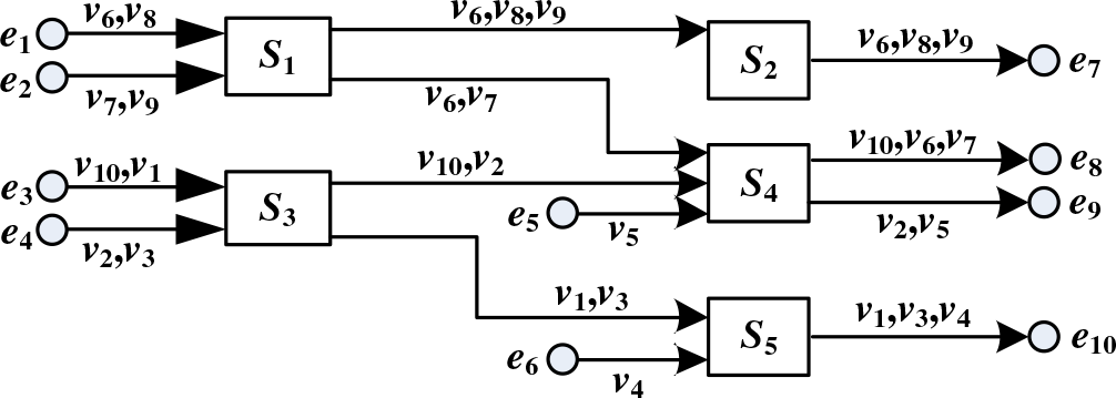
AFDX(3) is a packet-switched network based on Ethernet taking into account avionics constraints. It is an asynchronous and distributed network without global clock synchronisation. Full duplex connection ensures that there is no packet transmission collision on physical links. Each physical link has a maximum transmission speed (typically 100 Mb/s). Each switch has a FIFO buffer in every output port but no buffers in input ports. The delay incurred by the switching fabric is upper-bounded to a constant value. An illustrative example of an AFDX network is depicted in Fig. 1 which includes ten end systems (e 1 to e 10) and five switches (S 1 to S 5).
Illustrative AFDX network configuration.

Packet flows are transmitted through predefined logical paths which are called virtual links (VLs)(Reference Zhen, Feng and Zhang35,Reference Cha, Lim and Lee36) . A virtual link defines a logical and unidirectional connection from one transmitting end system to one or more receiving end systems. As the example in Fig. 1, v10 is a unicast VL with path  ${e_3} - {S_3} - {S_4} - {e_8}$
, while v 6 is a multicast VL with paths
 ${e_1} - {S_1} - {S_2} - {e_7}$
and
 ${e_1} - {S_1} - {S_4} - {e_8}$
. A virtual link is determined by the maximum packet length (F max) and the minimum time interval between the generations of two consecutive packets of a given VL. This minimum time interval is called Bandwidth Allocation Gap (BAG).
The deterministic behavior of the AFDX is ensured by traffic shaping and policy unit in each end system or switch. Typically, an industrial AFDX network includes more than one hundred end systems and two redundant AFDX sub networks, each composed of at least ten switches. Nearly 1000 VLs are transmitted on each sub network, corresponding to more than 6000 paths due to the multicast characteristic of VLs(Reference Scharbarg, Ridouard and Fraboul37).
4.0 FORWARD APPROACH
4.1 Modeling of network and traffic
A real-time avionics network is composed of a set of end systems and switches which are interconnected through physical links. Each multiplexing point (i.e. output port of an end system or a switch) can be modeled as a node. A node can be seen as a FIFO buffer which is working at the maximum servicing rate G = 100 Mb/s. All these nodes constitute a node set denoted as S = {N 1, N 2,…, N p}. The switching fabric delay is denoted as L which is upper-bounded to 16µs(Reference Kemayo, Ridouard and Bauer8,Reference Benammar, Ridouard and Bauer16) .
Packet flows transmitting through switches are composed of a flow set denoted as Г = {v 1,v 2,…,v n}. The subset  ${\Gamma_h}$
includes all the flows passing through node h. The transmission path
 ${{\mathscr{P}}_i}$
of flow v i is statically defined as an ordered node list from the source node (first i) to the destination node (last i). Here, the source node (first i) is the transmitting end system where the flows are generated. The destination node (last i) is not the receiving end system but the output port of the last visited switch along the transmission path
 ${{\mathscr{P}}_i}$
.
Generally, a flow v i can be characterised as follows:
• C i, the maximum transmission time of a packet generated by flow v i. It is equal to the maximum packet length
${F_{max}}$
divided by the switch servicing rate G:
\begin{align*}{C_i} = {{{F_{max}}} \over G}\end{align*}
• T i, the minimum time interval between two consecutive packets generated by flow v i. It corresponds to the BAG of a given VL in AFDX.
•
${{\mathscr{P}}_i}$
, the transmission path of flow v i. An ordered list of the crossed nodes from the source node (first i) to the destination node (last i).• L, the switching fabric delay. It is upper-bounded to 16µs.


The Forward Approach can be used for any other networks which can be abstracted as this model, only if all the flows have the same characteristics above.
4.2 Principles
Provided that m i is a packet generated by flow v i, in order to compute the worst-case end-to-end transmission delay, the Forward Approach (FA) iteratively analyses the maximum backlog at each node of path  ${{\mathscr{P}}_i}$
. It estimates the maximum transversal delay from the generation time at its source node to the departure time from each visited node h of path
 ${{\mathscr{P}}_i}$
. We denote this delay
 $R_i^h$
. The estimation propagates until the destination node (last i), so that the worst-case end-to-end transmission delay can be computed(Reference Kemayo, Ridouard and Bauer8).
DEFINITION 1 For any node h of path  ${{\mathscr{P}}_i}$
, the term
 $Smax_i^h$
is the maximum transmission delay for a packet of flow v ifrom its generation time at the source node (first i) to its arrive time at node h.
DEFINITION 2 For any node h of path  ${{\mathscr{P}}_i}$
, the term
 $Smin_i^h$
is the minimum transmission delay for a packet of flow v ifrom its generation time at the source node (first i) to its arrival time at node h.
DEFINITION 3 Backlog is defined as the total transmission time of all the pending packets in an output buffer at a given time. We define  ${\rm{Bklg}}_{\rm{i}}^{\rm{h}}$
the total transmission time of the maximum pending packets in the output buffer of node h when packet m iarrives.
Suppose node h belongs to path  ${{\mathscr{P}}_i}$
, and node h + 1 follows node h along path
 ${{\mathscr{P}}_i}$
. As each node follows the FIFO scheduling policy without considering priority, packet m i cannot be delayed by the packets arriving after itself,
 $S{\rm{max}}_i^h$
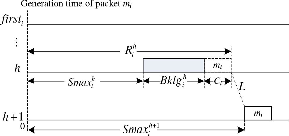
can be estimated iteratively as depicted in Fig. 2(Reference Kemayo, Ridouard and Bauer8,Reference Kemayo, Benammar and Ridouard12) .
Iterative estimation of  $S{\rm{max}}_i^h$
and
 $R_i^h$
.

We define the generation time of packet m i at the source node (first i) is the origin time, so that we have  $S\!\max _i^{\,firs{t_i}} = S\!\min _i^{\,firs{t_i}} = 0$
.
 $S{\rm{max}}_i^{h{\rm{ + 1}}}$
can be obtained as below if getting the value of
 $S{\rm{max}}_i^h$
(Reference Kemayo, Ridouard and Bauer8):
 \begin{align}S\!\max\nolimits_i^{h + 1} = S\!\max\nolimits_i^h\, + \,Bklg_i^h\, + \,{C_i}\, + \,L\end{align}
This computation propagates until the destination node (last i), the worst-case end-to-end delay R i of the packet m i is equal to the maximum transversal delay  $R_i^{las{t_i}}$
. It can be expressed as Eq. (2).
 \begin{align}{R_i} = R_i^{las{t_i}} = S\!\max\nolimits_i^{las{t_i}}\, + \,Bklg _i^{las{t_i}}\, + \,{C_i}\end{align}
To compute an upper bound of the end-to-end transmission delay of flow v i we need to determine the maximum backlog  $Bklg_i^h$
at each node h along path
 ${{\mathscr{P}}_i}$
.
For  $S{\rm{min}}_i^h$
, it occurs if there are no pending packets in the output buffer when packet m i arrives. Thus packet m i can be immediately forwarded once it arrives. When there is no backlog at each visited node,
 $S{\rm{min}}_i^h$
can be obtained as Eq. (3) where
 ${\left| h \right|^i}$
denotes the number of nodes crossed by packet m i from first ito h:
 \begin{align}\left\{ \begin{array}{ll}{S{\rm{min}}_i^{h{\rm{ + 1}}} = S{\rm{min}}_i^h + {C_{{\rm{i}}}} + L} \\[5pt] {{\rm{}}S{\rm{min}}_i^h = \left( {{{\left| h \right|}^i} - 1} \right) \times \left( {{C_i} + L} \right)} \end{array} \right.\end{align}
The Forward Approach (FA) evaluates the maximum backlog  $Bklg_i^h$
at each node h along path m i using
 $S{\rm{min}}_i^h$
and
 $S{\rm{max}}_i^h$
, and the worst-case end-to-end transmission delay R i can be computed(Reference Benammar, Ridouard and Bauer16).
4.3 Worst-Case scenario with the maximum backlog
This section presents the worst-case scenario which can construct the maximum backlog. We focus on packet m i generated by flow v i. The maximum backlog  $Bklg_i^h$
which can delay packet m i at node h is bounded by the time window from its earliest arrival time (
 $S{\rm{min}}_i^h$
) to its latest arrival time (
 $S{\rm{max}}_i^h$
).
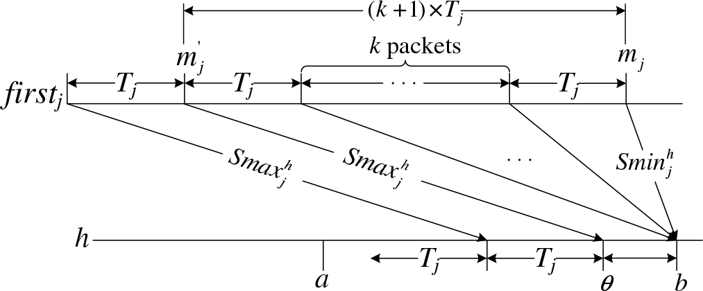
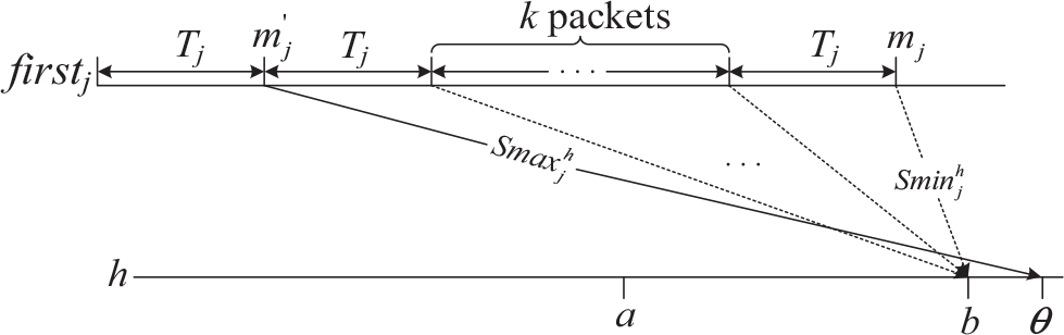
THEOREM 1 The maximum backlog generated by an interfering flow v j at node h during a time interval [a, b] occurs in the scenario as below(Reference Kemayo, Ridouard and Bauer8):
(i). Packets of flow v j should be generated at the maximum rate from its source node (first j).
(ii). All the packets of flow v j arriving at node h in the time interval [a, b] constitute a packet sequence
$\omega$
, suppose that m j is the last packet of
$\omega$
, it has to arrive at node h strictly at the end of this time interval, i.e. the time instant b.(iii). The last packet m j arrives at node h suffering the minimum delay (
$S{\rm{min}}_j^h$
). In the packet sequence
$\omega$
there is another packet
$m^{\prime}_{j}$
before m j, it is the last packet which arrives at node h earlier than m j suffering the maximum delay (
$S{\rm{max}}_j^h$
).(iv). All the packets before
$ {\text{m}}^{\prime}_{\text{j}}$
in the packet sequence
$\omega$
arrive at node h suffering the maximum delay (
$S{\rm{max}}_j^h$
).(v). Suppose that there are k packets between
$m^{\prime}_{j}$
and m j. All these k packets arrive at node h simultaneously with packet m j.


The corresponding worst-case scenario is depicted as Fig. 3.
Worst-case scenario that packet m jarrives at node h simultaneously with other k previous packets.

Proof To construct the maximum backlog, the interfering flow v j should generate the maximum competing traffic. To achieve this, packets of flow v j should be generated at the source node (first j) as quickly as possible, hence, flow v j should generate packets at the minimum time interval T j, which proves item (i).
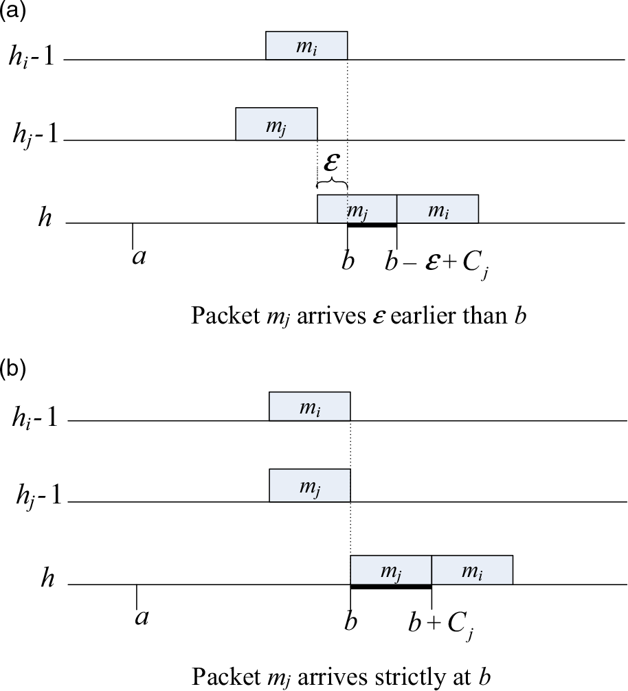
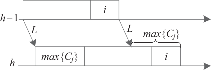
Suppose packet m j of flow v j arrives at node h  $\varepsilon$
earlier than b. When packet m i arrives at node h strictly at time b as depicted in Fig. 4 (a), it can be forwarded at time
 $b + {C_j} - \varepsilon $
. It means packet m i suffers
 ${C_j} - \varepsilon $
delay which is marked as a black bar. If packet m j of flow v j arrives at node h strictly at time b as depicted in Fig. 4 (b), when packet m i arrives at node h strictly at time b, it can be forwarded at time
 $b + {C_j}$
. It means packet m i suffers
 ${C_j}$
delay (also marked as a black bar) which is longer than
 ${C_j} - \varepsilon $
.
Packet m j delays packet m i.

No matter how earlier than b packet m j arrives at node h, there is always a worse scenario that packet m j arrives at node h strictly at time b, and this scenario can cause a longer delay to packet m i. Item (ii) is proved.
If the last packet m j arrives at node h suffering a delay d ( $S{\rm{min}}_i^h \lt d \lt S{\rm{max}}_i^h$
), the time difference between the arrivals of the last two packets (m j and its previous packet) in the packet sequence
 $\omega$
is larger than when packet m j arrives suffering the minimum delay
 $S{\rm{min}}_i^h$
, so that the backlog is not maximised. Some packets in the packet sequence
 $\omega$
will not arrive simultaneously with packet m j. To ensure the maximum backlog they should suffer the maximum delay to arrive at node h. Item (iii) is proved.
Since packet  $m^{\prime}_{j}$
arrives at node h in the time interval [a,b] suffering the maximum delay
 $S{\rm{max}}_j^h$
, to ensure more packets can arrive at node h during this time interval, all the packets before
 $m^{\prime}_{j}$
have to suffer the maximum delay
 $S{\rm{max}}_j^h$
. Item (iv) is proved.
For item (v), these k packets arrive at node h no earlier than  $m^{\prime}_{j}$
, based on item (ii) they should arrive at node h simultaneously with m j to ensure the maximum delay to packet m i. The last item is proved.
Generally, we can analyse the packet sequence  $\omega$
from back to front.
• The last packet m j arrives at node h strictly at the end of the time interval [a,b], suffering the minimum delay
${\rm{}}S{\rm{min}}_j^h$
.• There are k packets before packet m j, these k packets arrive at node h simultaneously with packet m j suffering different delays between (
$S{\rm{min}}_j^h$
,
$S{\rm{max}}_j^h$
).• There is a packet
$m^{\prime}_{j}$
arriving at node h earlier than the end of the time interval [a,b], suffering the maximum delay
$S{\rm{max}}_j^h$
.• The other packets before
$m^{\prime}_{j}$
in the packet sequence
$\omega$
arrive at node h suffering the maximum delay
$S{\rm{max}}_j^h$
.


THEOREM 2 (Reference Kemayo, Ridouard and Bauer8) The difference of the arrival times at node h between packets  $m^{\prime}_{j}$
and m j is not longer than the minimum packet generation interval T j.
Proof Suppose that packet  $m^{\prime}_{j}$
arrives at node h at time
 $\theta$
depicted in Fig. 3. From item (ii) and (iii) we have
 $\theta$
< b. Packet
 $m^{\prime}_{j}$
suffers the maximum delay
 $S{\rm{max}}_j^h$
. The next packet is generated T j after
 $m^{\prime}_{j}$
, and it won’t suffers a delay longer than
 $S{\rm{max}}_j^h$
, so that the arrival time difference between those two packet (
 $m^{\prime}_{j}$
and the following one) is not longer than T j. This following packet arrives at node h simultaneously with packet m j, thus the arrival time difference between packets
 $m^{\prime}_{j}$
and m jis not longer than T j. Theorem 2 is proved.
THEOREM 3 (Reference Kemayo, Ridouard and Bauer8) All the packets before  $m^{\prime}_{j}$
arrive at node h periodically with a time interval T j.
Proof Item (iv) demonstrates that all the packets before  $m^{\prime}_{j}$
arrive at node h suffering the maximum delay
 $S{\rm{max}}_j^h$
. Since packet
 $m^{\prime}_{j}$
also suffers the maximum delay, and their generation interval is T j, so that they arrive at node h one after another with a time interval T j. Theorem 3 is proved.
4.4 Request bound function
The maximum backlog generated by flow v j at node h during a time interval [a,b] has been presented in Theorem 1. In order to determine this backlog, we define the Request Bound Function (RBF) and the cumulative function W(t) in this section.
The Request Bound Function  $RBF_j^h{\rm{(}}t{\rm{)}}$
defines the total transmission time of packets generated by flow v j arriving at node h during a time interval of length
 $t(t{\rm{ }} = {\rm{ }}b - a)$
. The cumulative function
 ${W^h}{\rm{(}}t{\rm{)}}$
defines the total transmission time of packets generated by all the flows passing through node h during a time interval of length t. We have(Reference Kemayo, Ridouard and Bauer8):
 \begin{align}{{\rm{W}}^{\rm{h}}}{\rm{(t)}} = \sum\nolimits_{{\rm{v}}_{\rm{j}}\in _{\Gamma_{\rm{h}}}} {{\rm{RBF}}_{\rm{j}}^{\rm{h}}{\rm{(t)}}} \end{align}
The computation of  $RBF_j^h{\rm{(}}t{\rm{)}}$
has to be consistent with the scenario built as Theorem 1. As depicted in Fig. 3, the backlog at node h generated by flow v j is composed of two parts:
(a) The periodic part ending with packet
$m^{\prime}_{j}$
(
$m^{\prime}_{j}$
is included). Packets in this part arrive at node h one after another with a time interval T j.(b) The simultaneous part ending with packet m j (m jis included). Packets in this part arrive at node h simultaneously with m j.


LEMMA 1 (Reference Benammar, Ridouard and Bauer16) The maximum backlog generated by flow v j at node h is achieved when packet  $m^{\prime}_{j}$
arrives at node h at time
 $\theta$
. Suppose
 $\theta$
is
 ${\rm{\Delta }}_j^h$
earlier than b, we have:
 \begin{align}{\rm{\Delta }}_{\rm{j}}^{\rm{h}} = \left( {{\rm{k}} + 1} \right) \times {T_j} - {\rm{J}}_{\rm{j}}^{\rm{h}}\end{align}
Where  $J_j^h = S{\rm{max}}_j^h - S{\rm{min}}_j^h$
is the worst-case arrival jitter of flow v j, and k is the number of the packets arriving at node h simultaneously with packet m j.
Proof Consider the generation time of packet  $m^{\prime}_{j}$
as the reference time
 ${t_{ref}}$
. Its arrival time at node h can be expressed as:
 \begin{align}\theta = {{\rm{t}}_{{\rm{ref}}}}{\rm{}} + {\rm{Smax}}_{\rm{j}}^{\rm{h}}\end{align}
As there are k+1 time intervals T jfrom  $m^{\prime}_{j}$
to m j as depicted in Fig. 3, and packet m j arrives at node h suffering the minimum delay
 $S{\rm{min}}_j^h$
, the time instant b can be expressed as:
 \begin{align}{\rm{b}} = {{\rm{t}}_{{\rm{ref}}}} + {\rm{(k + 1) \times }}{{\rm{T}}_{\rm{j}}} + {\rm{Smin}}_{\rm{j}}^{\rm{h}} \end{align}
and Lemma 1 can be proved as below:
 \begin{align} {\rm{\Delta }}_j^h & = b - {\rm{}}\theta \nonumber\\
& = (k + 1) \times {T_j} + S{\rm{min}}_j^h - S{\rm{max}}_j^h \\
& = (\rm{k} + 1) \times {{\rm{T}}_{\rm{j}}} - {\rm{J}}_{\rm{j}}^{\rm{h}}\nonumber\end{align}
LEMMA 2 (Reference Kemayo, Ridouard and Bauer8) The obtained term  ${\rm{\Delta }}_j^h$
(c.f. Lemma 1) is always greater than zero:
 ${\rm{\Delta }}_j^h{\rm{ \gt 0}}$
.
Proof If  ${\rm{\Delta }}_j^h{ = \rm{ 0}}$
, it means that packet
 $m^{\prime}_{j}$
arrives at node h simultaneously with m j, this is contrary to item (iii) of Theorem 1 which demonstrates packet
 $m^{\prime}_{j}$
arrives earlier than m j. If
 ${\rm{\Delta }}_j^h{\rm{ \lt 0}}$
, it means that packet
 $m^{\prime}_{j}$
arrives at node h later than m j as depicted in Fig. 5. Packet m j is generated after
 $m^{\prime}_{j}$
, with the FIFO scheduling policy, it definitely arrives at node h after
 $m^{\prime}_{j}$
. It is impossible that
 ${\rm{\Delta }}_j^h{\rm{ \lt 0}}$
.
Packet  $m^{\prime}_{j}$
arrives later than m j.

LEMMA 3 (Reference Kemayo, Ridouard and Bauer8) Let k is the number of the packets arriving at node h simultaneously with packet m j. In the scenario with worst-case backlog, k satisfies:
 \begin{align}{\rm{k}}{{\rm{T}}_{\rm{j}}}{\rm{}} \le {\rm{J}}_{\rm{j}}^{\rm{h}}{\rm{ \lt (k + 1)}}{{\rm{T}}_{\rm{j}}}\end{align}
Proof LEMMA 2 has proved that  ${\rm{\Delta }}_j^h{\rm{ \gt 0}}$
, from Eq. (8) we can get
 ${\rm{(}}k{\rm{ + 1) \times }}{T_j} - J_j^h{\rm{ \gt 0}}$
, and
 $J_j^h{\rm{ \lt (}}k{\rm{ + 1)}}{T_j}$
, the right part of Eq. (9) is proved. Theorem 2 demonstrates that
 ${\rm{\Delta }}_j^h \le {T_j}$
, it means that
 ${\rm{(}}k{\rm{ + 1) \times }}{T_j} - J_j^h \le {T_j}$
, and
 $k{T_j} \le J_j^h$
, the left part of Eq. (9) is proved.
THEOREM 4 (Reference Benammar, Ridouard and Bauer16) The Request Bound Function  $RBF_j^h{\rm{(}}t{\rm{)}}$
for flow v j passing through node h in a time interval of length t (t > 0) is:
 \begin{align}{\rm{RBF}}_{\rm{j}}^{\rm{h}}{\rm{(t) = }}\left( {{\rm{1 + }}{{{\rm{t + J}}_{\rm{j}}^{\rm{h}}} \over {{{\rm{T}}_{\rm{j}}}}}} \right) \cdot {{\rm{C}}_{\rm{j}}}\end{align}
Proof We separately prove Eq. (10) for two different parts: the periodic part ending with packet  $m^{\prime}_{j}$
and the simultaneous part ending with packet m j.
When length t is shorter than  ${\rm{\Delta }}_j^h$
, the maximum count of the pending packets is k+1 (packet m j and the k packets arriving simultaneously with itself as depicted in Fig. 3). From Eq. (9), we have
 $k{T_j} \le J_j^h$
, so that
 $k{T_j} \le t + J_j^h$
. Since t is shorter than
 ${\rm{\Delta }}_j^h$
, we have
 $t + J_j^h \lt J_j^h + \Delta_j^h$
. From Eq. (8) we have
 $J_j^h{\rm{ + \Delta }}_j^h{ = \rm{ (}}k{\rm{ + 1) \times }}{T_j}$
, so that
 $t + J_j^h{\rm{ \lt (}}k{\rm{ + 1) \times }}{T_j}$
. We have:
 \begin{align} & k{T_j} \le t + J_j^h \lt \left( {k + {\rm{1}}} \right) \cdot {T_j}\nonumber \\
& \quad\Leftrightarrow k \le {{t + J_j^h} \over {{T_j}}} \lt \left( {k + {\rm{1}}} \right)\\
& \quad\Leftrightarrow \,\Bigg\lfloor {{{t + J_j^h} \over {{T_j}}}} \Bigg\rfloor = k \nonumber\end{align}
so that Eq. (10) can get the maximum backlog for any time interval  $t{\rm{ (}}0 \lt t{\rm{ \lt \Delta }}_j^h)$
.
When the length t is  ${\rm{\Delta }}_j^h$
, the maximum count of the pending packets is k+2 (packet m j, the k packets arriving simultaneously with itself and packet
 $m^{\prime}_{j}$
as depicted in Fig. 3). We have:
 \begin{align} t + J_j^h & = \Delta _j^h + J_j^h \nonumber\\
& = \left( {k + {\rm{1}}} \right) \cdot {T_j} \\
& \Leftrightarrow \Bigg\lfloor{{t + J_j^h} \over {{T_j}}}\Bigg\rfloor = k{\rm{ + 1}} \nonumber\end{align}
Eq. (10) can get the maximum backlog for time interval  $t = \Delta _j^h$
. and
 $t + J_j^h$
is multiple of T j.
When the length t is longer than  ${\rm{\Delta }}_j^h$
, one new packet can arrive every T j because all the packets before
 $m^{\prime}_{j}$
arrive at node h one after another every T j.
All the analysis above proves Theorem 4.
COROLLARY 1 Eq. (10) defined in theorem 4 is identical at the source node to the total transmission time of the pending packets generated by flow v j during a time interval of length t (Reference Kemayo, Ridouard and Bauer8,Reference Benammar, Ridouard and Bauer16) .
Proof By the definition, at the source node, we have  $S{\rm{min}}_j^{\,firs{t_j}} = S{\rm{max}}_j^{\,firs{t_j}} = 0$
. Therefore,
 $J_j^{\,firs{t_j}} = 0$
and Eq. (10) can be expressed as:
 \begin{align}{\rm{RBF}}_{\rm{j}}^{\rm{h}}{\rm{(t) = }}\left( {{\rm{1 + }}\left\lfloor {{{\rm{t}} \over {{{\rm{T}}_{\rm{j}}}}}} \right\rfloor } \right) \cdot {{\rm{C}}_{\rm{j}}}\end{align}
As illustrated by Corollary 1, at the source node, every  ${T_j}$
time interval one new packet of flow v j can be generated. There is only the periodic arriving part at the source node.
With the Request Bound Function  $RBF_j^h{\rm{(}}t{\rm{)}}$
computed by Eq. (10), we can obtain the total transmission time
 ${W^h}{\rm{(}}t{\rm{)}}$
for the packets generated by all the interfering flows during a time interval of length t. On one hand, the competing packets arrive forming the backlog at node h, on the other hand, the arrived packets are being forwarded leaving node h, so that the available time to forward those packets should be subtracted. Furthermore, Fig. 2 and Eq. (1) demonstrate that packet m i is included in the computation of
 $S{\rm{max}}_i^{h{\rm{ + 1}}}$
, the transmission time C i should be subtracted in the computation of the maximum backlog
 $Bklg_i^h$
. We have:
 \begin{align}{{Bklg}}_{\rm{i}}^{\rm{h}}{ = \rm{ ma}}{{\rm{x}}_{{\rm{t}} \ge {\rm{0}}}}\left( {{{\rm{W}}^{\rm{h}}}\left( {\rm{t}} \right) - {{\rm{C}}_{\rm{i}}} - {\rm{t}}} \right)\end{align}
COROLLARY 2  $Bklg_i^h$
computed by Eq. (14) is never negative(Reference Kemayo, Ridouard and Bauer8).
Proof When there is only one flow v i without any interfering flows, for the minimum time interval t = 0, we can obtain  ${W^h}(0) - {C_i}{\rm{ - 0 = 0}}$
. This is the minimum backlog. However,
 $Bklg_i^h$
corresponds to the maximum value of this computation, so it cannot be negative.
4.5 Stop condition
To compute the maximum backlog  $Bklg_i^h$
encountered by flow v i at node h, The time interval of any possible length t should be tested. It is necessary to determine a maximum length as the stop condition of this test to ensure the maximum backlog is included. We denote this maximum length of the time interval as
 ${\mathscr{B}^h}$
. To determine the maximum length, we separately take into account the two parts in Section 4.4, the periodic part and the simultaneous part.
For the periodic part, we introduce the concept of busy period(Reference Qingfei and Xinyu25,Reference Bauer, Scharbarg and Fraboul32) . The backlog is included in a busy period. A busy period is a time interval between two consecutive idle time instants which are respectively the starting time and the ending time of this busy period. An idle time instant means all the pending packets have been forwarded (there is no backlog at this idle time instant). Therefore, packets arrived before an idle time instant should not be included in the computation of the backlog for the following busy period. Consequently, the computation of the backlog should end with the first following idle time instant (the ending time of the busy period), as the packets arrived after the idle time instant cannot generate any backlog.
LEMMA 4 (Reference Kemayo, Benammar and Ridouard12) The length of the maximum busy period at node h generated by flow set  ${\Gamma_h}$
is bounded to the first positive value satisfying the following equation if
 $\sum\nolimits_{j \in {{\rm{}}_h}} {{{{C_j}} \over {{T_j}}} \le {\rm{1}}} $
.
 \begin{align}\left\{ \begin{array}{ll} {{\mathscr{B}}{{\mathscr{P}}^{\rm{h}}}(0) = \sum\nolimits_{{\rm{j}} \in {{\rm{}}_{\rm{h}}}} {{{\rm{C}}_{\rm{j}}}} } \\
{{\mathscr{B}}{{\mathscr{P}}^{\rm{h}}}\left( {{\rm{k + 1}}} \right) = \sum\nolimits_{{\rm{j}} \in {{\rm{}}_{\rm{h}}}} {\left\lceil {{{{\mathscr{B}}{{\mathscr{P}}^{\rm{h}}}({\rm k})} \over {{{\rm{T}}_{\rm{j}}}}}} \right\rceil \cdot {{\rm{C}}_{\rm{j}}}} }
\end{array} \right.\end{align}
This computation ends with the first positive value satisfying  ${\mathscr{BP}}^h\left( {k{\rm{ + 1}}} \right) = {\mathscr{BP}}^h\left( k \right)$
.
This longest busy period represents the maximum time interval between two consecutive idle time instants. Therefore, for the periodic part of a flow, if the length of a time interval is larger or equal to the longest busy period  ${\mathscr{BP}}^h$
, the computation of the backlog can be stopped as an idle time exists(Reference Kemayo, Ridouard and Bauer8).
For the simultaneous part, as depicted in Lemma 1,  ${\rm{\Delta }}_j^h$
represents the length of the simultaneous part. Generally,
 ${\rm{ma}}{{\rm{x}}_{j\in{\Gamma _h}}}(\Delta _j^h)$
can include all the simultaneous parts of the flows passing through node h.
 ${\rm{\Delta }}_j^h$
can be determined by Lemma 5 when knowing the maximum jitter
 $J_j^h$
.
LEMMA 5 (Reference Benammar, Ridouard and Bauer16) For any flow v j passing through node h, we have:
 \begin{align}{\rm{\Delta }}_{\rm{j}}^{\rm{h}} = {\rm{}}\left( {1 + \left\lfloor {{{{\rm{J}}_{\rm{j}}^{\rm{h}}} \over {{{\rm{T}}_{\rm{j}}}}}} \right\rfloor } \right) \cdot {{\rm{T}}_{\rm{j}}} - {\rm{J}}_{\rm{j}}^{\rm{h}}\end{align}
Proof From Eq. (8) we obtain  ${\rm{\Delta }}_j^h{ = \rm{ (}}k{\rm{ + 1) \times }}{T_j} - J_j^h$
, where k is the number of the packets arriving simultaneously with packet m j,
 $J_j^h$
is the maximum arrival jitter (
 $J_j^h = S{\rm{max}}_j^h - S{\rm{min}}_j^h$
). From Eq. (9) we have:
 \begin{align} & k{T_j} \le J_j^h \lt \left( {k + {\rm{1}}} \right) \cdot {T_j} \nonumber\\
& \quad \Leftrightarrow k \le {{J_j^h} \over {{T_j}}} \lt \left( {k + {\rm{1}}} \right) \\
& \quad \Leftrightarrow \left\lfloor {{{J_j^h} \over {{T_j}}}} \right\rfloor = k \nonumber\end{align}
Replacing k with  $\left\lfloor {{{J_j^h} \over {{T_j}}}} \right\rfloor $
in Eq. (8) proves Lemma 5.
The maximum length of the time interval containing all simultaneous parts can be limited to  ${\mathscr{B}}{{{S}}^{\rm{h}}}$
:
 \begin{align}{\mathscr{B}}{{\rm{S}}^{\rm{h}}} = \mathop {\max }\limits_{{v_j} \in {\Gamma _h}} \left\{ {\left( {1 + \left\lfloor {{{J_j^h} \over {{T_j}}}} \right\rfloor } \right) \cdot {T_j} - J_j^h} \right\}\end{align}
The two lemmas above determine the maximum length of the time interval for computing the worst-case backlog respectively considering the periodic and simultaneous part.
THEOREM 5 (Reference Kemayo, Ridouard and Bauer8) Suppose a set of flows Гh passing through node h, if  $\sum\nolimits_{j \in {{\rm{\Gamma}}_h}} {{{{C_j}} \over {{T_j}}} \le {\rm{1}}} $
and node h follows the FIFO servicing policy, the maximum length of the test time interval can be expressed as:
 \begin{align}{\mathscr{B}^h} = \mathscr{B}{P^h} + \mathscr{B}{S^h}\end{align}
Proof Lemma 4 and 5 prove this theorem.
For each flow  $v_i{\rm{}} \in \Gamma$
and each node h of path
 $\mathscr{P}_{i}$
, an upper bound of the worst-case transversal delay
 $R_i^h$
can be obtained by
 \begin{align}{\rm{R}}_{\rm{i}}^{\rm{h}} = S{\rm{max}}_{\rm{i}}^{\rm{h}}+ Bklg_{\rm{i}}^{\rm{h}} + {{\rm{C}}_{\rm{i}}}\end{align}
The maximum backlog  $Bklg_i^h$
can be computed according to Eq. (21)
 \begin{align}{{Bklg}}_{\rm{i}}^{\rm{h}} = \rm{ ma}{{\rm{x}}_{{{\mathscr{B}}^{\rm{h}}} \ge {\rm{t}} \ge 0}}\left( {{{\rm{W}}^{\rm{h}}}\left( {\rm{t}} \right) - {{\rm{C}}_{\rm{i}}} - {\rm{t}}} \right)\end{align}
With  ${W^h}(t)$
being defined by Eq. (4). The computation ends with
 ${{\mathscr{B}}^h}$
which is obtained by Eq. (19).
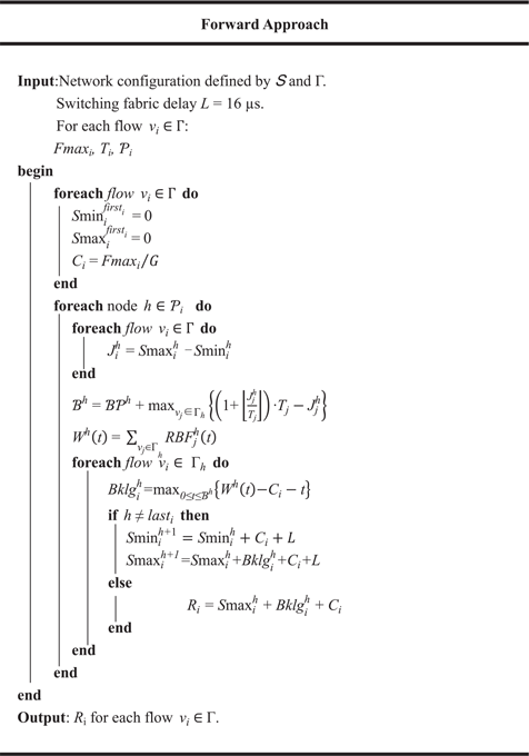
The pseudo-code for the Forward Approach is given by Algorithm 1. In fact, the computation can be done in a discrete manner by testing time t only at arrival times of new packets(Reference Kemayo, Ridouard and Bauer8). This computation does not consider the serialisation effect.
Forward Approach without considering the serialisation effect.

4.6 Serialisation effect for forward approach
In packet switched networks such as AFDX, packets are necessarily serialised when being transmitted through a common physical link. Packets transmitted through a common physical link cannot arrive at the next switch simultaneously. They are serialised. This is what is commonly called the serialisation effect(Reference Kemayo, Benammar and Ridouard12).
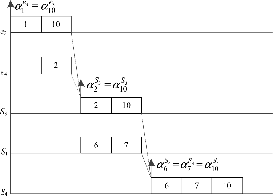
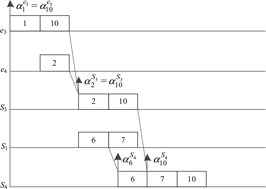
For example, consider flow v 10 in Fig. 1. Suppose packet i is generated by flow v i.  $\alpha _i^h$
indicates the arrival time at node h of packet i. According to the Forward Approach, the maximum backlog encountered by packet 10 at each node along its transmission path is depicted in Fig. 6. Packet 10 is delayed by packet 1 at its source node (e 3). At node S 3, it is delayed by packet 2 from node e 4. At node S 4, it is delayed by both packets 6 and 7 from node S 1. But this is impossible as packets 6 and 7 are transmitted through the same physical link. They are serialised and cannot arrive at node S 4 simultaneously. The actual worst-case end-to-end transmission delay for packet 10 is depicted in Fig. 7.
Maximum backlog for packet 10 on its transmission path according to the Forward Approach.

Actual worst-case end-to-end transmission delay for packet 10 along its transmission path.

Figure 7 shows that not both packets 6 and 7 can cause delay to packet 10. This demonstrates the maximum backlog computed by the Forward Approach is pessimistic (overestimated), thus the obtained upper bound of the end-to-end transmission delays is pessimistic (overestimated). The computation of the serialisation effect in this section can improve the Trajectory approach to ensure the tightness of the backlog as well as the delay upper bound.
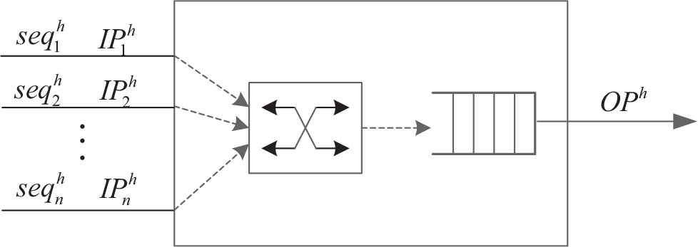
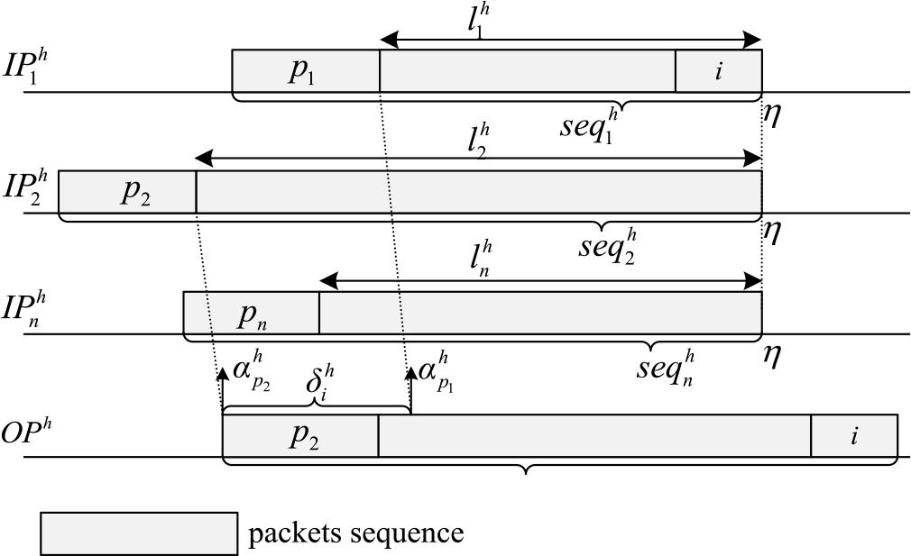
Consider node h with n input physical links as depicted in Fig. 8. Flows from n physical links are transmitted to the same output physical link  $O{P^h}$
. The n input physical links are respectively denoted as
 $IP_x^{h}$
where
 $x \in {\rm{}}\left\{ {{\rm{1, \ldots ,}}n} \right\}$
.
Node h with n input physical links.

The cumulative function W(t) can be obtained by summing the transmission time of the packets from each physical link  $IP_x^h$
. Suppose
 $W_x^h(t)$
is the transmission time of packets from the physical link
 $IP_x^{h}$
during a time interval of length t, so that we have(Reference Benammar, Ridouard and Bauer13,Reference Benammar, Ridouard and Bauer16) :
 \begin{align}{{\rm{W}}^{\rm{h}}}\!\left( {\rm{t}} \right) = \sum\nolimits_{{\rm{x}} = 1}^{\rm{n}} {{\rm{W}}_{\rm{x}}^{\rm{h}}\left( {\rm{t}} \right){\rm{}}}\end{align}
We need to determine the maximum value of each  $W_x^h(t)$
where
 $x \in {\rm{}}\left\{ {{\rm{1, \ldots ,}}n} \right\}$
. The fixed transmission rate of each virtual link in AFDX networks ensures the maximum account of the arrived packets during a time interval of length t. The expression of
 $W_x^h(t)$
thus can be determined.
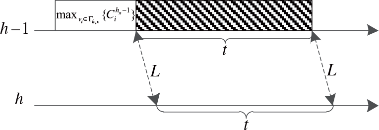
Worst-case cumulative transmission time of packets through an input link during a time interval of length t.

LEMMA 6 (Reference Kemayo, Benammar and Ridouard12) The worst-case transmission time of packets arriving at node h from the input physical link  $IP_x^{h}$
during a time interval of length t is limited to Eq. (23):
 \begin{align}{\rm{W}}_{\rm{x}}^{\rm{h}}\left( {\rm{t}} \right){\rm{}} \le {\rm{}}{{{{\rm{G}}^{{{\rm{h}}_{\rm{x}}} - {\rm{1}}}}} \over {{{\rm{G}}^{{{\rm{h}}_{\rm{x}}}}}}} \times {\rm{t}} + {\max _{{v_i} \in\Gamma {{\rm{}}_{{\rm{h,x}}}}}}\left\{ {{\rm{C}}_{\rm{i}}^{\rm{h}}} \right\}\end{align}
where ( ${h_x} - 1$
) is the predecessor of node h along the physical the link
 $IP_x^{h}$
.
Proof Nodes  ${h_x} - 1$
and h are directly connected through the physical link
 $IP_x^{h}$
. Therefore, the transmission time of packets at node h coming through the input link
 $IP_x^{h}$
is determined by the count of transmitted packets(Reference Benammar, Ridouard and Bauer16):
(1) During the time interval of length t, the count of packets transmitted to node h through
$IP_x^{h}$
is
${G^{{h_x} - {\rm{1}}}} \times t$
depicted as the shaded area in Fig. 9.(2) To ensure the worst-case, we suppose that a packet with the maximum length has been completely transmitted at the very beginning of this time interval,
${\max _{{v_i} \in\Gamma {{\rm{}}_{h,x}}}}\left\{ {C_i^{{h_x} - {\rm{1}}}} \right\}$
.


The worst-case transmission time of the packets coming through the input physical link  $IP_x^{h}$
during a time interval of length t is limited to Eq. (24) and Lemma 6 is proved.
 \begin{align}{{{{\rm{G}}^{{{\rm{h}}_{\rm{x}}}{\rm{ - 1}}}}{\rm{ \times t}}} \over {{{\rm{G}}^{\rm{h}}}}}{\rm{}} + {\max _{{{\rm{v}}_{\rm{i}}} \in\Gamma {{\rm{}}_{{\rm{h,x}}}}}}\left\{ {{\rm{C}}_{\rm{i}}^{\rm{h}}} \right\}\end{align}
THEOREM 6 (Reference Kemayo, Ridouard and Bauer8,Reference Benammar, Ridouard and Bauer16) The cumulative transmission time of the packets transmitted through the physical link  $IP_x^{h}$
during a time interval of length t at node h is bounded by
 \begin{align}{\rm{W}}_{\rm{x}}^{\rm{h}}\left( {\rm{t}} \right) = {\min _{}}\left\{ {\sum\nolimits_{{{\rm{v}}_{\rm{i}}} \in\Gamma {{\rm{}}_{{\rm{h,x}}}}} {{\rm{RBF}}_{\rm{i}}^{\rm{h}}{\rm{(t)}}} ,{{{{\rm{G}}^{{{\rm{h}}_{\rm{x}}}{\rm{ - 1}}}}{\rm{ \times t}}} \over {{{\rm{G}}^{\rm{h}}}}} + {{\max }_{{{\rm{v}}_{\rm{i}}} \in\Gamma {{\rm{}}_{{\rm{h,x}}}}}}\left\{ {{\rm{C}}_{\rm{i}}^{\rm{h}}} \right\}} \right\}\end{align}
Proof Eq. (4) and (23) define two guaranteed upper bounds of value  $W_x^h(t)$
, so it can be limited by the smaller value. Theorem 6 is proved.
There is exception for Theorem 6 at source node of flow v i. At the source node there is no serialisation effect, and  ${W^h}{\rm{(}}t{\rm{)}}$
should be computed only according to Eq. (4).
THEOREM 7 (Reference Benammar, Ridouard and Bauer16) If node h is the source node of flow v i, the cumulative transmission time W(t) should only be computed according to Eq. (4).
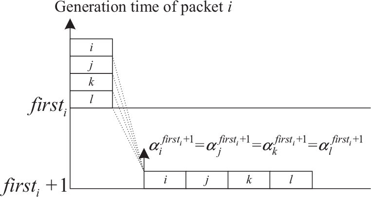
Proof At the source node (first i) of flow v i, all the flows are generated at this node instead of coming from input physical links. Packets are generated by different flows at the same time, and arrive at the output port simultaneously. As depicted in Fig. 10, suppose the source node (first i) of flow v i has three other flows such as flow j, k and l. and packets j, k and l arrive at the output port of node h simultaneously with packet i. There is no serialisation effect for these flows.
No serialisation effect for the packets generated at the source node.

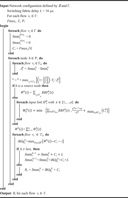
The pseudo-code of the Forward Approach integrated with the serialisation effect is given by Algorithm 2. The computation can also be done in a discrete manner by testing time t only at arrival times of new packets.
Forward Approach integrated with the serialisation effect

5.0 CASE STUDY AND COMPARISON
This section compares the Forward Approach with other approaches on sample AFDX configurations. The comparison is performed respectively with or without the serialisation effect. Through a case study we present the optimism existing in the computation of the serialisation effect. In the end of this section, we present a new computation of the serialisation effect.
5.1 Comparative analysis
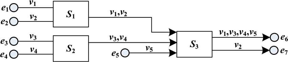
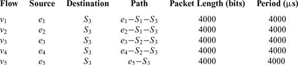
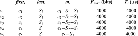
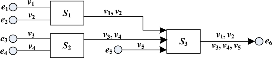
An illustrative AFDX network is depicted in Fig. 11. The flow characteristics are given in Table 1. As an example, we analyse flow  ${v_1}({\mathscr{P}_1} = {e_1} - {S_1} - {S_3})$
which meets flow v 2 at switch S 1, meets v 3, v 4 and v 5 at switch S 3.
Illustrative AFDX network.

Characteristics of flows

When not considering the serialisation effect, we should analyse all the nodes along path  $\mathscr{P}_{1}$
according to Algorithm 1. By definition, we have
 $S{\rm{min}}_{\rm{1}}^{{e_{\rm{1}}}} = S{\rm{max}}_{\rm{1}}^{{e_{\rm{1}}}}{ = \rm{ 0}}$
and the arrival jitter
 ${J^{{e_{\rm{1}}}}}$
is zero. As v 1 is the only flow emitted from e 1, the maximum backlog can be computed by Eq.(26):
 \begin{align}{{Bklg}}_{\rm{1}}^{{{\rm{e}}_{\rm{1}}}}{ = \rm{ ma}}{{\rm{x}}_{{\rm{0}} \le {\rm{t}} \le {{\mathscr{B}}^{{{\rm{e}}_{\rm{1}}}}}}}\left\{ {\left( {{\rm{1 + }}\left\lfloor {{{\rm{t}} \over {{{\rm{T}}_{\rm{1}}}}}} \right\rfloor } \right) \cdot {{\rm{C}}_{\rm{1}}} - {{\rm{C}}_{\rm{1}}}{\rm{ - t}}} \right\}\end{align}
According to Lemma 4 and 5, we have:
 \begin{align*}\mathscr{BP}^{{{\rm{e}}_{\rm{1}}}} = {{{C}}_{\rm{1}}} = {\rm{40}}\end{align*}
 \begin{align*}\mathscr{B}S^{{e_{\rm{1}}}} = \left( {{\rm{1 + }}\left\lfloor {{{{J^{{e_{\rm{1}}}}}} \over {{T_{\rm{1}}}}}} \right\rfloor } \right). T{\,_{\rm{1}}} = 4000{\rm{\mu s}}\end{align*}
where the arrival jitter  ${J^{{e_{\rm{1}}}}} = 0$
.
The length of the test interval is obtained as:
 \[{\rm{}}{\mathscr{B}^{{e_{\rm{1}}}}} = \mathscr{B}{\mathscr{P}^{{e_{\rm{1}}}}} + \mathscr{B}{S^{{e_{\rm{1}}}}} = {\rm{40 + 4000}} = {\rm{4040}}{\rm{\mu s}}\]
The maximum backlog is obtained at time t = 0. We have
 \begin{align*}Bklg_{\rm{1}}^{{e_{\rm{1}}}} = 0{\rm{\mu s}}\end{align*}
According to Eq. (1), we have
 \begin{align*}S{\rm{max}}_{\rm{1}}^{{S_1}}{ = \rm{ 40 + 16 = 56\mu s}}\end{align*}
According to Eq. (3), we can obtain
 \begin{align*}S{\rm{min}}_{\rm{1}}^{{S_1}}{ = \rm{ 40 + 16 = 56\mu s}}\end{align*}
The arrival jitter  ${J^{{S_1}}}$
is zero.
Similarly, we also have
 \begin{align*}S{\rm{max}}_{\rm{2}}^{{S_1}} = S{\rm{max}}_2^{{S_1}} = {\rm{56\mu s}}\end{align*}
and the arrival jitter is zero, too.
At node S 1, flow v 1 meets v 2, the maximum backlog  ${\rm{}}Bklg_{\rm{1}}^{{S_1}}$
can be expressed as:
 \begin{align*}Bklg_{\rm{1}}^{{S_1}} = ma{x_{0 \le t \le {\mathscr{B}^{{{\rm{S}}_1}}}}}\left\{ {\left( {{\rm{1 + }}\left\lfloor {{t \over {{T_{\rm{1}}}}}} \right\rfloor } \right) \cdot {C_{\rm{1}}} + \left( {{\rm{1 + }}\left\lfloor {{t \over {{T_{\rm{2}}}}}} \right\rfloor } \right) \cdot {C_{\rm{2}}} - {C_{\rm{1}}} - t} \right\}\end{align*}
According to Lemma 4 and 5, we have:
 \begin{align*} \mathscr{B}{P^{{S_1}}} & = {C_{\rm{1}}} + {C_{\rm{2}}} = {\rm{80}}{\rm{\mu s}} \\
\mathscr{B}{S^{{S_1}}} & = \left( {{\rm{1 + }}\left\lfloor {{{{J^{{S_1}}}} \over {{T_{\rm{1}}}}}} \right\rfloor } \right) \cdot {T_{\rm{1}}} = 4000{\rm{\mu s}} \end{align*}
where the arrival jitter  ${J^{{S_1}}} = 0$
.
The length of the test interval is obtained as:
 \begin{align*}{\mathscr{B}^{{S_1}}} = \mathscr{B}{\mathscr{P}^{{S_1}}} + \mathscr{B}{S^{{S_1}}} = {\rm{80 + 4000 = 4080\mu s}}\end{align*}
The maximum backlog is obtained at time t = 0, and we have
 \begin{align*}Bklg_{\rm{1}}^{{S_1}} & = {\rm{40\mu s}}\\
S{\rm{max}}_{\rm{1}}^{{S_{\rm{3}}}} & = {\rm{56 + 40 + 40 + 16}} = {\rm{152\mu s}}\end{align*}
Finally, in the last node of  $\mathscr{P}_{1}$
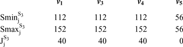
, flow v 1 meets v 3, v 4 and v 5. The values of
 $S{\rm{max}}_j^{{S_{\rm{3}}}}$
and
 $S{\rm{min}}_j^{{S_{\rm{3}}}}\left( {j = {\rm{1,3,4,5}}} \right)$
for those four flows are depicted in Table 2.
Durations to reach node S 3

The maximum backlog  $Bklg_{\rm{1}}^{{S_{\rm{3}}}}$
can be expressed as:
 \begin{align*}Bklg_{\rm{1}}^{{S_{\rm{3}}}} = & \mathop {max}\limits_{{\rm{0}} \le {\rm{t}} \le {\mathscr{B}^{{S_{\rm{3}}}}}} \left\{ \left( {{\rm{1 + }}\left\lfloor {{{t + J_1^{{S_{\rm{3}}}}} \over {{T_{\rm{1}}}}}} \right\rfloor } \right) \cdot {C_{\rm{1}}} + \left( {{\rm{1 + }}\left\lfloor {{{t + J_3^{{S_{\rm{3}}}}} \over {{T_3}}}} \right\rfloor } \right) \cdot {C_3} + \left( {{\rm{1 + }}\left\lfloor {{{t + J_4^{{S_{\rm{3}}}}} \over {{T_4}}}} \right\rfloor } \right) \cdot {C_4}\right.\\
& \left. + \left( {{\rm{1 + }}\left\lfloor {{{t + J_5^{{S_{\rm{3}}}}} \over {{T_5}}}} \right\rfloor } \right) \cdot {C_5} - {C_{\rm{1}}} - {\rm{t}} \right\}\end{align*}
According to Lemma 4 and 5, we have:
 \begin{align*}\mathscr{B}{\mathscr{P}^{{S_{\rm{3}}}}} = {C_{\rm{1}}} + {C_{\rm{3}}} + {C_4} + {C_{\rm{5}}} = {\rm{160}}{\rm{\mu s}}\end{align*}
 \begin{align*}{\mathscr{B}}{{\rm{S}}^{{{\rm{S}}_{\rm{3}}}}} = {\rm{}}\left( {{\rm{1 + }}\left\lfloor {{{{{\rm{J}}^{{{\rm{S}}_{\rm{3}}}}}} \over {{{\rm{T}}_{\rm{1}}}}}} \right\rfloor } \right)\,{ \cdot T_{\rm{1}}} = {\rm{4000\mu s}}\end{align*}
where the arrival jitter  ${J^{{S_{\rm{3}}}}} = 40{\rm{\mu s}}$
.
The length of the test interval is obtained as:
 \[{\mathscr{B}^{{S_{\rm{3}}}}} = \mathscr{B}{\mathscr{P}^{{S_{\rm{3}}}}} + \mathscr{B}{S^{{S_{\rm{3}}}}} = {\rm{160 + 4000 = 4160\mu s}}\]
The maximum backlog encountered by flow v 1 at node S 3 is obtained at time t = 0, and  $Bklg_{\rm{1}}^{{S_{\rm{3}}}} = {\rm{120\mu s}}$
.
The worst-case end-to-end transmission delay of flow v 1 is
 \begin{align} R1= S{\rm{max}}_{\rm{1}}^{{S_{\rm{3}}}} + Bklg_{\rm{1}}^{{S_{\rm{3}}}} + {C_{\rm{1}}}{\rm{}} = {\rm{152}} + {\rm{120}} + {\rm{40}} = {\rm{312\mu s}} \end{align}
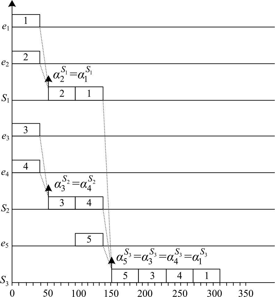
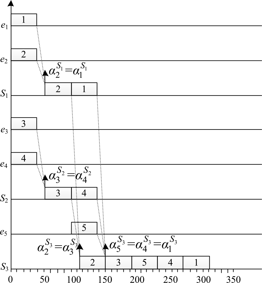
The corresponding scenario of the worst-case transmission is depicted in Fig. 12.
Worst-case scenario corresponding to the Forward Approach without considering serialisation effect.

When considering the serialisation effect, at the source node, the cumulative function  ${W^h}(t)$
is computed according to Theorem 6 and 7. As there is only one flow at node e 1, the cumulative transmission time is computed by
 \begin{align}{{\rm{W}}^{{{\rm{e}}_{\rm{1}}}}}\!\left( {\rm{t}} \right){ = \rm{ ma}}{{\rm{x}}_{0 \le {\rm{t}} \le {{\rm{B}}^{{{\rm{e}}_1}}}}}\left\{ {\left( {{\rm{1 + }}\left\lfloor {{{\rm{t}} \over {{{\rm{T}}_{\rm{1}}}}}} \right\rfloor } \right) \cdot {{\rm{C}}_{\rm{1}}}{\rm{ - t}}} \right\} \end{align}
The maximum value is 40 which is obtained at time t = 0. The maximum backlog
 \begin{align} Bklg_{\rm{1}}^{{e_{\rm{1}}}} = {W^{{e_{\rm{1}}}}}(0) - {C_{\rm{1}}}{ = \rm{ 40}} - {\rm{40 = 0}} \end{align}
We have
 \begin{align*} S{\rm{max}}_{\rm{1}}^{{S_1}}{ = \rm{ 40 + 16 = 56\mu s}}\end{align*}
and
 \begin{align*} S{\rm{min}}_{\rm{1}}^{{S_1}}{ = \rm{ 40 + 16 = 56\mu s}} \end{align*}
The arrival jitter is zero. Similarly, we also have  $S{\rm{max}}_{\rm{2}}^{{S_1}} = S{\rm{max}}_{\rm{2}}^{{S_1}} = {\rm{56\mu s}}$
, and the arrival jitter is zero too.
Then v 1 and v 2 meet at node S 1. The maximum cumulative transmission time is computed as
 \begin{align}{{\rm{W}}^{{{\rm{S}}_1}}}\!\left( {\rm{t}} \right){\rm{}} = {\rm{mi}}{{\rm{n}}_{}}\left\{ {\left( {{\rm{1 + }}\left\lfloor {{{\rm{t}} \over {{{\rm{T}}_{\rm{1}}}}}} \right\rfloor } \right) \cdot {{\rm{C}}_{\rm{1}}}{\rm{,t}} + {{\rm{C}}_{\rm{1}}}} \right\} + {\min _{}}\left\{ {\left( {{\rm{1 + }}\left\lfloor {{{\rm{t}} \over {{{\rm{T}}_{\rm{2}}}}}} \right\rfloor } \right) \cdot {{\rm{C}}_{\rm{2}}}{\rm{,t}} + {{\rm{C}}_{\rm{2}}}} \right\} \end{align}
The maximum value is obtained at time t = 0 and the maximum backlog
 \begin{align} Bklg_{\rm{1}}^{{S_1}} = {W^{{S_1}}}(0) - {C_{\rm{1}}}{ = \rm{ 80}} - {\rm{40 = 40\mu s}} \end{align}
We have
 \begin{align*} S{\rm{max}}_{\rm{1}}^{{S_{\rm{3}}}} &= S{\rm{max}}_{\rm{1}}^{{S_1}} + Bklg_{\rm{1}}^{{S_1}} + {C_{\rm{1}}} + L \\ & = 56 + 40 + 40 + 16 \\ &= 152\mu \rm{s} \end{align*}
Then v 1 meets v 3, v 4 and v 5 at node S 3. Flows v 3 and v 4 are coming through the same physical link, they are serialised. The maximum cumulative transmission time is computed as
 \begin{align}{W^{{S_{\rm{3}}}}}(t) &= \mathop {\min }\limits_{} \left\{ {\left( {{\rm{1 + }}\left\lfloor {{t \over {{T_{\rm{1}}}}}} \right\rfloor } \right) \cdot {C_{\rm{1}}}{\rm{,}}t + {C_{\rm{1}}}} \right\}\mathop { + \min }\limits_{} \left\{ \left( {{\rm{1 + }}\left\lfloor {{t \over {{T_{\rm{4}}}}}} \right\rfloor } \right) \cdot {C_{\rm{4}}} + \left( {{\rm{1 + }}\left\lfloor {{t \over {{T_{\rm{3}}}}}} \right\rfloor } \right) \cdot {C_{\rm{3}}}{\rm{,}}t \right.\nonumber\\
&\quad\left.+ \mathop {\max }\limits_{} \left\{ {{C_{\rm{3}}},{C_{\rm{4}}}} \right\} \right\} + {\min _{}}\left\{ {\left( {{\rm{1 + }}\left\lfloor {{{\rm{t}} \over {{{\rm{T}}_{\rm{5}}}}}} \right\rfloor } \right) \cdot {{\rm{C}}_{\rm{5}}}{\rm{,t}} + {{\rm{C}}_{\rm{5}}}} \right\}\end{align}
The maximum value is 120µs which is obtained at time t = 0. The corresponding maximum backlog is
 \begin{align}Bklg_{\rm{1}}^{{S_{\rm{3}}}} = {W^{{S_{\rm{3}}}}}(0) - {C_{\rm{1}}}{ = \rm{ 120}} - {\rm{40 = 80\mu s}}\end{align}
The worst-case end-to-end transmission delay is:
 \begin{align}{\rm{}}{R_1} = S{\rm{max}}_{\rm{1}}^{{S_{\rm{3}}}} + {\rm{}}Bklg_{\rm{1}}^{{S_{\rm{3}}}} + {C_1} = 152{\rm{ }} + {\rm{ }}80{\rm{ }} + {\rm{ }}40{\rm{ }} = {\rm{ }}272{\rm{ \mu s}}\end{align}
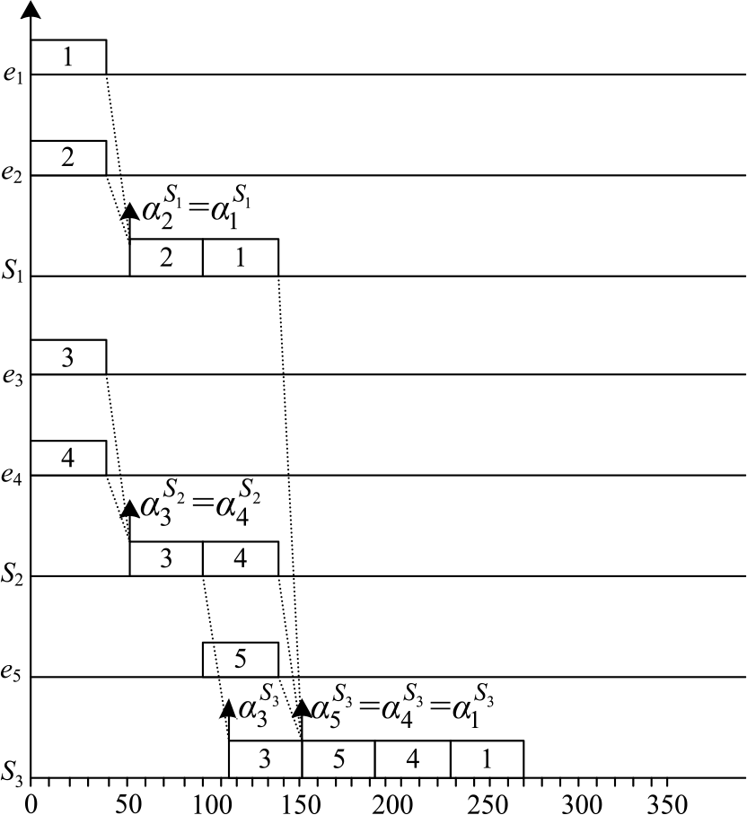
The corresponding scenario of the worst-case transmission is depicted in Fig. 13.
Compared with the transmission scenario depicted in Fig. 12, packets 3 and 4 cannot arrive at S 3 simultaneously with packet 1 in Fig. 13. One of them arrives 40µs earlier and does not cause delay to packet 1 (packet 3 arrives 40µs earlier in Fig. 13, it is similar if packet 4 arrives earlier). That is why the worst-case end-to-end transmission delay computed in Eq. (27) has 40µs pessimism compared with Eq. (34).
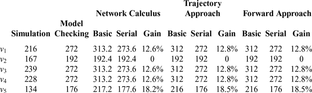
Similarly, the worst-case end-to-end transmission delays of the other flows in Table 1 are given in Table 3. We can see, compared with the Forward Approach without considering the serialisation effect, the Forward Approach integrated with the serialisation effect can compute a tighter upper bound for flows v 1, v 3, v 4 and v 5. Flow v 2 has no gains as there is no serialisation effect during its transmission. Compared with the Network Calculus approach and the Trajectory Approach, the Forward Approach can obtain a tighter upper bound than the Network Calculus approach, it and can keep the same tightness as the Trajectory Approach no matter with or without the serialisation effect. Moreover, when compared with the Model Checking approach, we find that the Forward Approach integrated with the serialisation effect can obtain the exact delay upper bounds for all the flows in the network configuration of this experiment. The simulation method usually obtains an optimistic upper bound due to missing some rare scenarios, and it is not necessary to do the comparative analysis between the simulation method and the Forward Approach integrated with the serialisation effect.
Worst-case end-to-end transmission delays

Basic: computed without the serialisation effect.
Serial: computed with the serialisation effect.
Gain: improvement when considering the serialisation effect.
Worst-case scenario corresponding to the Forward Approach integrated with the serialisation effect.

5.2 Optimism in serialisation computation
In this section, we present the potential optimism existing in the computation of the serialisation effect, which is given in Section 4.6. An illustrative AFDX network is depicted in Fig. 14. The only difference with Fig. 11 is that flow v 2 is transmitted to e 6 in this figure. The flow characteristics are given in Table 4. It is the same as Table 1.
Characteristics of flows

An illustrative AFDX network.

We still focus on flow v 1 which is transmitted from e 1 to e 6. Flow v 1 meets v 2 at node S 1, meets v 3, v 4 and v 5 at node S 3.
At the source node e 1, there is only flow v 1, and the backlog at node e 1 is zero. The corresponding computation is similar to Eq. (28) and (29). We have:
 \begin{align*}S{\rm{min}}_{\rm{1}}^{{S_1}} = S{\rm{max}}_{\rm{1}}^{{S_1}}{ = \rm{ 40 + 16 = 56\mu s}}\end{align*}
At node S 1,  $Bklg_{\rm{1}}^{{S_1}} = 40$
µs, the corresponding computation is similar to Eq. (30) and (31). We can obtain:
 \begin{align*}S{\rm{max}}_{\rm{1}}^{{S_{\rm{3}}}} = S{\rm{max}}_{\rm{1}}^{{S_1}} + Bklg_{\rm{1}}^{{S_1}} + {C_1} + L = {\rm{56 + 40 + 40 + 16 = 152\mu s}}\end{align*}
At node S 3,  $Bklg_{\rm{1}}^{{S_{\rm{3}}}} = {\rm{80}}$
µs, the corresponding computation is similar to Eq. (32) and (33).
The worst-case end-to-end transmission delay is 272µs as computed in Eq. (34).
In fact, for flow v 1, the exact worst-case end-to-end transmission delay is 312µs as depicted in Fig. 15.
In this configuration, both packets 3 and 4 can cause delay to packet 1 even they do not arrive at node S 3 simultaneously with packet 1 (in fact, packet 3 arrives 40µs earlier than packet 1, packet 4 arrives simultaneously with packet 1). The actual backlog at node S 3 is
 \begin{align*}Bklg_1^{{S_3}} = {{\rm{C}}_{\rm{3}}} + {{\rm{C}}_{\rm{4}}} + {{\rm{C}}_{\rm{5}}}{ = \rm{ 120 \mu s}}\end{align*}
However, the backlog computed by Eq. (32) and (33) is only 80µs. It has 40µs optimism. This demonstrates that the computation of the serialisation effect presented in Section 4.6 computes an optimistic upper bound.
Actual worst-case end-to-end transmission delay.

5.3 New computation of serialisation effect
For the network configuration in Fig. 14, packet 3 can delay packet 1 even it does not arrive at node S 3 simultaneously with packet 1 (in fact, it arrives 40µs earlier, it arrives at node S 3 simultaneously with packet 2). In Fig. 15, we can see packets 3, 4 and 5 (all the packets coming from the other input physical inks) arrive at node S 3 not earlier than packet 2.
As depicted in Fig. 8, node h has n input physical links. Packets at the input link  $IP_x^{h}$
form a packet sequence
 $seq_x^{h}$
. Suppose flow v i are transmitted through the first input physical link
 $IP_1^h$
.
Due to the FIFO scheduling policy, any packet arriving at node h later than packet i cannot delay it. In order to maximise the delay of packet i at node h, each competing packet sequence is postponed and it finishes at the same time as the packet sequence  $seq_1^{h}$
. The finishing time is denoted as
 $\eta$
depicted in Fig. 16.
 $\delta _i^h$
is the maximum time difference between arrival of the first packet from
 $seq_x^{h}$
where
 $ x \in \{ 2, \ldots ,n\}$
and the arrival of the first packet from
 $seq_{\rm{1}}^{h}$
. Suppose p i is the first packet in the sequence
 $seq_x^{h}$
. In Fig. 16,
 $\delta _i^h$
is the time difference between the arrivals of packets p 2 and p 1.
Illustration of  ${\delta ^h}$
.

Packets in  $\delta _i^h$
are transmitted before p 1, and cannot cause any delay to packet i. The delay at node h suffered by packet i can be maximised when
 $\delta _i^h$
is minimised. For the computation of the worst-case end-to-end transmission delay, it comes to determine the minimum value of
 $\delta _i^h$
at each visited node h. it is obvious that the minimum value of
 $\delta _i^h$
is obtained by minimising
 $\alpha _{{p_{\rm{1}}}}^h$
and maximising
 $\alpha _{{p_x}}^h$
where
 $x{\rm{}} \in {\rm{\{ 2, \ldots ,}}n{\rm{\} }}$
.
Let us define  $l_x^h\,\left( {{\rm{1}} \le {\rm{}}x{\rm{}} \le {\rm{}}n} \right)$
is the transmission time of the packet sequence
 $seq_x^{h}$
without its first packet, from Fig. 16, we can obtain:
 $$\matrix{{\alpha _{{p_x}}^h = {\rm{ }}\eta - l_x^h + L} \hfill \cr} $$
and when x = 1 we have
 $$\matrix{{\alpha _{{p_1}}^h = {\rm{}}\eta - l_1^h + L} \hfill \cr} $$
Consequently, minimising  $\alpha _{{p_{\rm{1}}}}^h$
comes to maximise
 $l_1^h$
. It is obtained when the first packet is the smallest one in the packet sequence
 $seq_{\rm{1}}^{h}$
. Similarly, maximising
 $\alpha _{{p_x}}^h$
comes to minimise each
 $l_x^h$
for
 $\left( {{\rm{2}} \le {\rm{}}x{\rm{}} \le {\rm{}}n} \right)$
. It is obtained when the first packet is the largest one in the respective sequence.
To summarise,  $\delta _i^h$
can be lower bounded by the maximum of 0 and Eq. (37).
 \begin{align}ma{x_{{\rm{2}} \le {{x}} \le {{n}}}}{\rm{(}}mi{n_{}}{\rm{(}}l_x^h{\rm{))}} - ma{x_{}}{\rm{(}}l_1^h{\rm{)}}\end{align}
The new computation of the serialisation effect can be expressed by Eq. (38).
For the cumulative transmission time caused by the packets from the same physical link as flow v i, it is always limited to the transmission time of the maximum packet in this physical link as depicted in Fig. 17.
Maximum cumulative transmission time.

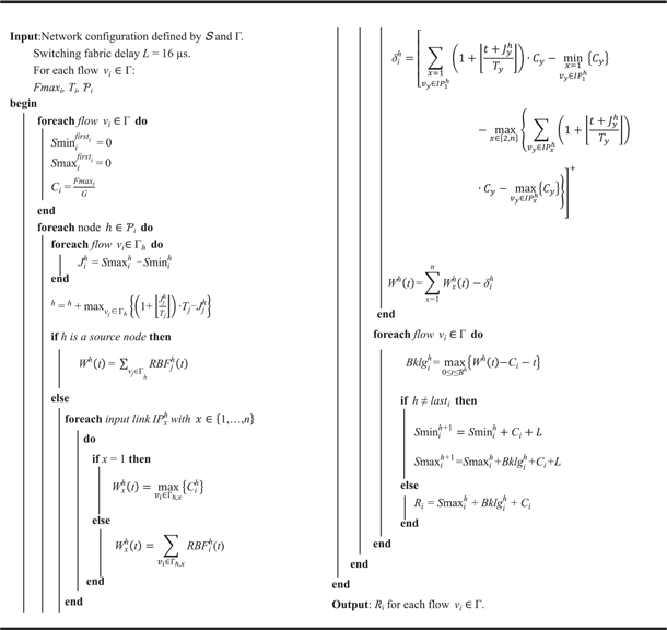
The pseudo-code for the Forward Approach integrated with the new computation of the serialisation effect is given by Algorithm 3. In fact, the computation can also be done in a discrete manner by testing time t only at arrival times of new packets.
 \begin{align}{\rm{\delta }}_{\rm{i}}^{\rm{h}} & = \left[ \mathop {{\rm{max}}}\limits_{{\rm{x}} \in \left[ {{\rm{2,n}}} \right]} \left( {\sum\nolimits_{{{\rm{v}}_{\rm{y}}} \in {\rm{IP}}_{\rm{x}}^{\rm{h}}} {\left( {1 + \left\lfloor {{{{\rm{t}} + {\rm{J}}_{\rm{y}}^{\rm{h}}} \over {{{\rm{T}}_{\rm{y}}}}}} \right\rfloor } \right)} \cdot {{\rm{C}}_{\rm{y}}} - {{\max }_{{{\rm{v}}_{\rm{y}}} \in {\rm{IP}}_{\rm{x}}^{\rm{h}}}}\left( {{{\rm{C}}_{\rm{y}}}} \right)} \right)\right. \nonumber\\ &\quad\left. - \left( {\sum\nolimits_{{{\rm{v}}_{\rm{y}}} \in {\rm{IP}}_{\rm{1}}^{\rm{h}}} {\left( {1 + \left\lfloor {{{{\rm{t}} + {\rm{J}}_{\rm{y}}^{\rm{h}}} \over {{{\rm{T}}_{\rm{y}}}}}} \right\rfloor } \right)} \cdot {{\rm{C}}_{\rm{y}}} - {{\min }_{{{\rm{v}}_{\rm{y}}} \in {\rm{IP}}_{\rm{1}}^{\rm{h}}}}\left( {{{\rm{C}}_{\rm{y}}}} \right)} \right) \right]^{+} \end{align}
Forward Approach integrated with the new computation of the serialisation effect

6.0 EXPERIMENTAL ANALYSIS
This section validates the new computation of the serialisation effect. We perform the experiments on both illustrative AFDX networks and real avionics systems.
6.1 Delays on illustrative AFDX networks
For the network configuration depicted in Fig. 14, we still focus on flow v 1.
At the source node e 1, there is only flow v 1, and the backlog at node e 1 is zero. The corresponding computation is similar to Eq. (28) and (29). We also have
 \begin{align*}S{\rm{min}}_{\rm{1}}^{{S_1}} = S{\rm{max}}_{\rm{1}}^{{S_1}}{ = \rm{ 40 + 16 = 56\mu s}}\end{align*}
At node S 1, there are two input physical links, for  $IP_{\rm{1}}^{{S_1}}$
, according to our new computation of the serialisation effect, the maximum cumulative transmission time is
 \begin{align*}W_{\rm{1}}^{{S_1}}{ = \rm{ max\{ }}{C_{\rm{1}}}{\rm{\} = 40\mu s}}\end{align*}
For  $IP_{\rm{2}}^{{S_1}}$
, the maximum cumulative transmission time
 \[{\rm{}}W_{\rm{2}}^{{S_1}} = \left( {{\rm{1 + }}\left\lfloor {{t \over {{T_{\rm{2}}}}}} \right\rfloor } \right) \cdot {C_{\rm{2}}} = 40{\rm{\mu s}}\]
As C 1 and C 2 arrive at node S 1 simultaneously, the serialisation effect at node S 1 $\delta _{\rm{1}}^{{S_1}} = 0$
. The maximum cumulative transmission time
 \[{{W}}_{}^{{{{S}}_1}}{ = { W}}_1^{{{{S}}_1}} + {{W}}_{{2}}^{{{{S}}_1}} - {\rm{\delta }}_{\rm{1}}^{{{{S}}_1}}{ = \rm{ 40 + 40}} - {\rm{0}} = \,80{\rm{\mu s}}\]
and the maximum backlog can be expressed:
 \begin{align*}Bklg_1^{{S_1}} = {\rm{}}W_{}^{{S_1}} - {{\rm{C}}_1} - t{\rm{}} = {\rm{80}} - {\rm{40}} = {\rm{40\mu s}}\end{align*}
We can have:
 \begin{align*}Smax_{\rm{1}}^{{S_{\rm{3}}}} = Smax_{\rm{1}}^{{S_1}} + Bklg_{\rm{1}}^{{S_1}} + {{\rm{C}}_1}{\rm{ + L}} = {\rm{56 + 40 + 40 + 16 = 152\mu s}}\end{align*}
At node S 3, there are three input physical links, for  $IP_{\rm{1}}^{{S_{\rm{3}}}}$
, the maximum cumulative transmission time
 \[W_{\rm{1}}^{{S_1}}{ = \rm{ max\{ }}{C_{\rm{1}}}{\rm{\} = 40}}{\rm{\mu s}}\]
For  $IP_{\rm{2}}^{{S_{\rm{3}}}}$
, the maximum cumulative transmission time is
 \begin{align*}W_{\rm{2}}^{{S_1}} = \left( {{\rm{1 + }}\left\lfloor {{t \over {{T_3}}}} \right\rfloor } \right) \cdot {C_{\rm{3}}} + \left( {{\rm{1 + }}\left\lfloor {{t \over {{T_{\rm{4}}}}}} \right\rfloor } \right) \cdot {C_4}{ = \rm{ 80\mu s}}\end{align*}
For  $IP_{\rm{3}}^{{S_{\rm{3}}}}$
, the maximum cumulative transmission time
 \[W_{\rm{3}}^{{S_1}} = \max \{ {C_5}\} = 40{\rm{\mu s}}\]
Packet 3 arrives at node S 3 earlier than packet 4, it arrives simultaneously with packet 2, so the serialisation effect at node S 3 $\delta _{\rm{1}}^{{S_{\rm{3}}}} = {\rm{0}}$
. The maximum cumulative transmission time is
 \[W_{}^{{S_{\rm{3}}}} = W_{\rm{1}}^{{S_{\rm{3}}}} + {\rm{}}W_{\rm{2}}^{{S_{\rm{3}}}} + {\rm{}}W_{\rm{3}}^{{S_{\rm{3}}}}{ = \rm{ 40 + 80 + 40 = 160\mu s}}\]
and the maximum backlog can be computed as below:
 \[Bklg_i^h = W_{}^{{S_3}} - {C_1} - t = 160 - 40 = 120{\rm{\mu s}}\]
The worst-case end-to-end transmission delay is:
 \[{R_{\rm{1}}} = S{\rm{max}}_{\rm{1}}^{{S_{\rm{3}}}} + {\rm{}}Bklg_{\rm{1}}^{{S_{\rm{3}}}} + {C_{\rm{1}}} = {\rm{152}} + {\rm{120}} + {\rm{40}} = {\rm{312\mu s}}\]
Compared with the original computation of the serialisation effect in Section 4.6, this new computation eliminates the optimism in Section 5.2. The obtained result is consistent with Fig. 15.
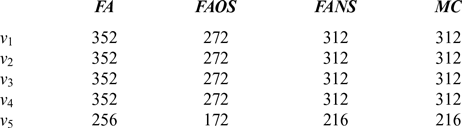
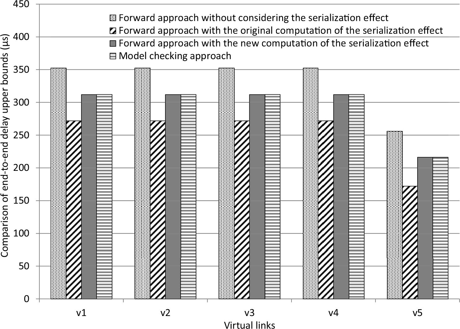
The upper bounds of other flows computed with different approaches are given in Table 5. The comparison histogram is depicted in Fig. 18.
Upper bounds of end-to-end transmission delay

FA: Forward Approach without considering the serialisation effect.
FAOS: Forward Approach with original serialisation.
FANS: Forward Approach with new serialisation.
MC: Model Checking approach.
Comparison of delay upper bounds obtained with different approaches.

6.2 Delays on real avionics systems
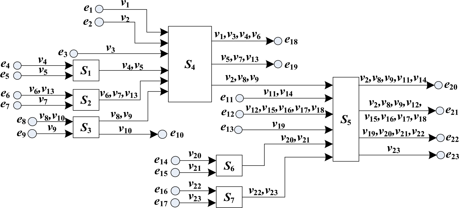
This section evaluates the new computation of the serialisation effect on a small real avionics network depicted in Fig. 19. It includes 23 end systems, 7 switches and 23 virtual links corresponding to 26 paths due to the multicast characteristic. All the VLs have a common traffic feature (BAG = 4000μs, C = 40μs). The technological latency is 16μs.
A small real avionics network.

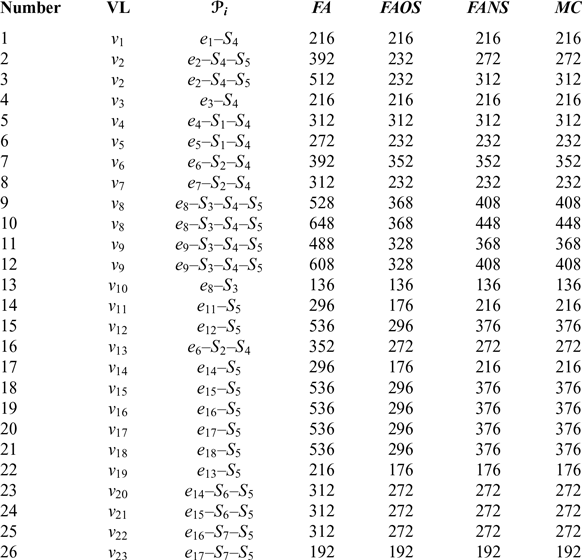
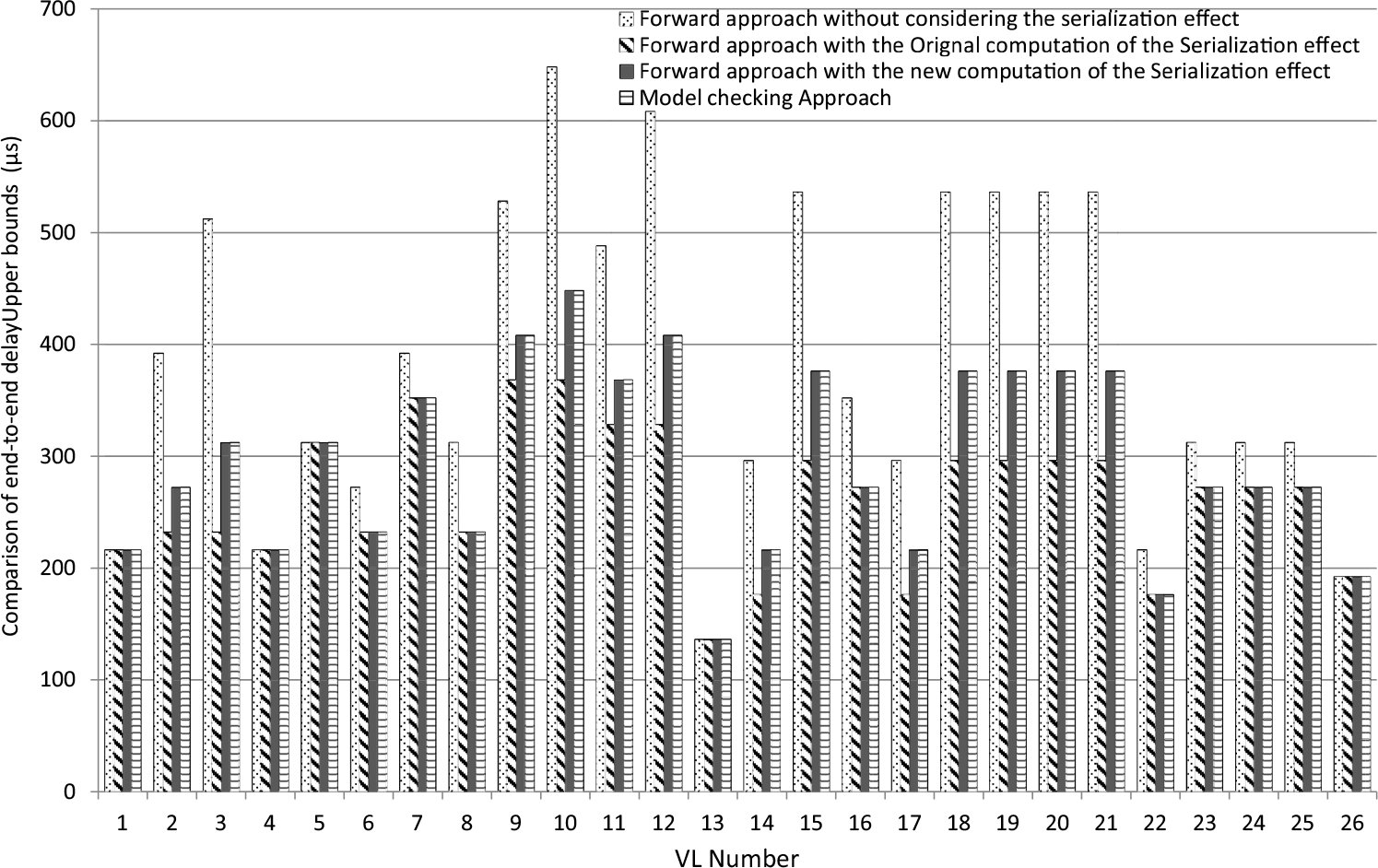
The worst-case end-to-end transmission delays computed with different approaches are summarised in Table 6, and the comparison is depicted in Fig. 20. The results obtained by the Model Checking approach are used as a reference.
Delay upper bounds computed with different approaches

FA: Forward Approach. FAOS: Forward Approach with original serialisation.
MC: Model Checking approach. FANS: Forward Approach with new serialisation.
Comparison of delay upper bounds computed with different approaches.

For all these flows, FANS can compute the exact worst-case end-to-end delays.
For flows v 1, v 3, v 4, v 10, v 23, FA, FAOS and FANS can compute the exact worst-case end-to-end delays, as no serialisation effect occurs during the whole transmission, and no pessimism is involved during the computation.
For flows v 5, v 6, v 7, v 13, v 19, v 20, v 21 and v 22, FA computes pessimistic upper bounds. FAOS and FANS can compute the exact worst-case end-to-end delays. It demonstrates that both the original computation of the serialisation effect and the new computation of the serialisation effect can eliminate the pessimism in the computation.
For flows v 2, v 8, v 9, v 11, v 12, v 14, v 15, v 16, v 17 and v 18, FA computes pessimistic upper bounds. FAOS computes optimistic upper bounds. It demonstrates FAOS involves optimism when eliminating the pessimism. However, FANS can compute the exact worst-case end-to-end transmission delays, it demonstrates that FANS eliminate the pessimism and does not involve the optimism in the original computation of the serialisation effect.
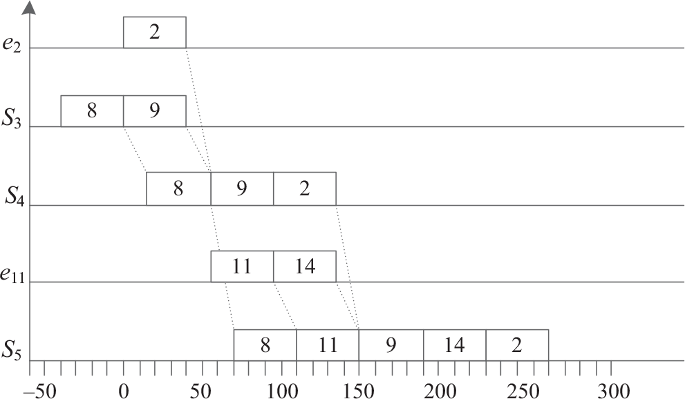
For example, flow v 2 with path  ${e_2} - {S_4} - {S_5}$
. The exact worst-case end-to-end transmission delay is 272μs as depicted in Fig. 21. FAOS eliminates the pessimism at S 4, but involves optimism at S 5 as it considers only one packet from e 11 can delay packet 2. In fact, both packets 14 and 11 can delay packet 2.
Delay upper bound of flow v 2.

Both the experiments on the illustrative AFDX network and the real avionics system demonstrate that the new computation of the serialisation effect can eliminate the pessimism in the Forward Approach and does not induce the optimism existing in the original computation of the serialisation effect.
7.0 Conclusion
This paper introduces the Forward Approach (FA) which is used to compute upper bounds of the end-to-end transmission delays for flows in avionics real-time networks such as AFDX. This approach is pessimistic (overestimated) as two packets transmitted through a common physical link cannot arrive at the next switch simultaneously. They are serialised. This sequential transmission is called the serialisation effect. The Forward Approach can obtain a tighter upper bound while considering the serialisation effect. Recently, our research finds that the computation of the serialisation effect might obtain an optimistic (underestimated) upper bound.
We propose a new computation of the serialisation effect in this paper. The results obtained by the Model Checking approach are used as a reference; the comparative experiments are performed on both a sample AFDX network and a small real avionics system. The comparative analysis demonstrates the new computation of the serialisation effect can eliminate the pessimism in the Forward Approach and does not induce the optimism existing in the original computation of the serialisation effect.
In future research, we will measure the scalability of the new computation of the serialisation effect. Meanwhile, we need to extend this approach to other servicing policies such as fix priorities of flows.
Data availability
The data used to support the findings of this study are included within the article.
Conflicts of interest
The authors declare that there is no conflict of interest regarding the publication of this paper.
Funding statement
This work is sponsored by the China 1000 Young Talents Program, the Young Talent Support Plan of Xi’an Jiaotong University, NSF China (NSFC) under Grants 61772410 and 61572398. The work is also sponsored by the China Post-Doctoral Science Foundation under Grant 2015M570837 and the National Natural Science Foundation of China (NSFC) under Grant No. 61502381.
Acknowledgements
This paper is written with the help from CPA&DCS Bus Test and Validation Laboratory of Shanghai Aviation Electric Co., Ltd. The authors would like to thank Yunrui Zhang and his research team for their inspirational discussions.

Qingfei Xu earned his master degree in Computer Science from Xi’an JiaoTong University in 2009. He is working at Shanghai Aviation Electric co. LTD, and currently pursuing PhD degree in Xi’an JiaoTong University. His research interests include avionics, network architecture, and communication reliability and performance evaluation