1 Introduction
Transient growth (TG) has been proposed as a mechanism responsible for subcritical transition in wall-bounded shear flows. Ellingsen & Palm (Reference Ellingsen and Palm1975) have shown that for an inviscid fluid, the streamwise component of a three-dimensional (3-D) streamwise independent disturbance grows linearly with time. Later on, Landahl (Reference Landahl1980) has shown that at long times, the kinetic energy will grow at least linearly with time. Gustavsson (Reference Gustavsson1991) has shown that inclusion of viscosity leads to decay of the initial growth and also distinguished between symmetric and antisymmetric disturbances. During the TG, the base flow may be modified significantly and become unstable to infinitesimal secondary disturbances. Gustavsson (Reference Gustavsson1991) has also shown that the relevant time parameter for the TG development is of
 $O(Re)$
and that two parameters are sufficient to characterize the TG: the total wavenumber
 $k=\sqrt{\unicode[STIX]{x1D6FC}^{2}+\unicode[STIX]{x1D6FD}^{2}}$
and the product
 $\unicode[STIX]{x1D6FC}Re$
, where
 $\unicode[STIX]{x1D6FC}$
and
 $\unicode[STIX]{x1D6FD}$
are the streamwise and spanwise wavenumbers, respectively and
 $Re$
is the Reynolds number, defined as
 $Re=U_{ref}h/\unicode[STIX]{x1D708}$
, where
 $U_{ref}$
is the centreline velocity,
 $U_{c}$
, for plane Poiseuille flow (PPF) and the velocity of the wall,
 $U_{w}$
, for plane Couette flow (PCF),
 $h$
is half the channel height and
 $\unicode[STIX]{x1D708}$
is the fluid kinematic viscosity.
The first to carry out a thorough investigation of the linear TG mechanism in PPF and PCF were Butler & Farrell (Reference Butler and Farrell1992). They have performed a parametric study revealing the optimal streamwise and spanwise wavenumbers leading to the maximal energy gain. They have found that the most efficient TG occurs for a nearly streamwise independent counter-rotating vortex pair (CVP) having a spanwise wavenumber of
 $\unicode[STIX]{x1D6FD}=2$
for PPF and
 $\unicode[STIX]{x1D6FD}=1.67$
for PCF. Two types of optimal disturbances were identified, symmetric (even) TG which generates a symmetric streamwise velocity distribution with respect to the
 $y$
axis and antisymmetric (odd) TG which generates an antisymmetric streamwise velocity distribution with respect to the
 $y$
axis. For PCF the even TG corresponds to a pair of vortices (single CVP), whereas the odd TG corresponds to two pairs of vortices (2 CVPs), one pair at the upper half and the second at the lower half of the channel.
Streamwise independent vortices generate streamwise velocity streaks which may become unstable to secondary instabilities. Therefore, the research progressed to secondary instability studies of streamwise independent vortices. Lundbladh, Henningson & Reddy (Reference Lundbladh, Henningson, Reddy and Hussaini1994) have calculated the transition thresholds in PPF and PCF based on a combination of a primary disturbance and small amplitude noise as a secondary disturbance. The primary disturbances were streamwise independent vortices (even and odd) with
 $\unicode[STIX]{x1D6FD}=2$
and oblique waves with
 $\unicode[STIX]{x1D6FC}=1$
and
 $\unicode[STIX]{x1D6FD}=1$
which generate streamwise independent vortices with
 $\unicode[STIX]{x1D6FD}=2$
. The choice of
 $\unicode[STIX]{x1D6FD}=2$
is based on the fact that it corresponds to maximal growth for PPF (and almost maximal growth for PCF for which
 $\unicode[STIX]{x1D6FD}=1.67$
). The sensitivity of the results to the spanwise wavenumber has not been examined. Surprisingly, the odd TG (which grows much less in energy) was found to have a lower threshold for transition compared to the one for the even TG, suggesting that maximal energy growth is not essential for transition.
The self-sustained process proposed by Waleffe (Reference Waleffe1995) contains secondary instability of streamwise streaks as one of the stages. The process has been derived for PCF and the secondary instabilities have been identified to be sinuous (wake type) associated with spanwise inflection points. As a model for the streak instability the author assumed that the vortices (rolls) are artificially maintained so that at a certain time the streamwise velocity reaches a steady state where the lift-up effect is balanced by viscous dissipation. The sinuous instability of the most amplified TG (single CVP,
 $\unicode[STIX]{x1D6FD}=1.67$
) has been analysed but the full parametric study has been left for future work. In a subsequent study by Waleffe (Reference Waleffe1997), steady rolls and streaks, obtained after one quarter of the roll’s turnover time, have been used in the stability analysis as they are maintained on average during the self-sustained process. Results only for
 $\unicode[STIX]{x1D6FD}=1.67$
are shown, corresponding to previous studies. In real flow the vortices and streaks are unsteady. Studying the effects of flow unsteadiness and various spanwise wavenumbers is valuable to better understand the streak instability phase.
Reddy et al. (Reference Reddy, Schmid, Baggett and Henningson1998) have performed a thorough investigation of streak instability for PCF and PPF and compared the threshold energies for transition for streamwise vortices, oblique waves, Tollmien–Schlichting waves and two-dimensional optimals. For PCF only symmetric TG (single CVP) and
 $\unicode[STIX]{x1D6FD}=2$
have been analysed. They have found that sinuous secondary disturbances are the most dangerous ones except at very low CVP magnitudes. Comparison with antisymmetric TG and analysis of various spanwise wavenumbers are necessary to generalize their conclusions. Park & Huerre (Reference Park and Huerre1995) have investigated the primary and secondary instabilities of streaks in an asymptotic suction boundary layer on a curved plate. They have demonstrated the existence of varicose and sinuous instability modes, associated with wall-normal and spanwise shear, respectively. They have found that for
 $\unicode[STIX]{x1D6FD}=0.5$
the sinuous mode is the most dangerous one due to the strong spanwise inflection points. They have noted that the spanwise wavenumber plays a decisive role in the type of the instability, however, the effect of
 $\unicode[STIX]{x1D6FD}$
has not been studied. Sinuous instability has also been identified as the dominant one by Andersson et al. (Reference Andersson, Brandt, Bottaro and Henningson2001) who have studied numerically streak instability in a laminar boundary layer. Asai, Minagawa & Nishioka (Reference Asai, Minagawa and Nishioka2002) have studied the instability properties of a single streak experimentally. They have demonstrated that both varicose and sinuous modes can be excited and compared their growth rates. The growth rate of the varicose mode has been found to be very sensitive to the streak width (i.e.
 $\unicode[STIX]{x1D6FD}$
), whereas the growth rate of the sinuous mode remained fairly constant. It can be seen that sometimes the sinuous modes are the most dangerous ones whereas in other cases the varicose modes are more dominant. Without analysing all possible spanwise wavenumbers it is hard to know which of the modes is the most dangerous one. We aim to fill this gap for TG in PCF in the current work.
More recent works have concentrated on nonlinear optimal disturbances such as the minimal seed and the edge state. Contrary to the linear optimals which are elongated in the streamwise direction and span through the entire channel, the nonlinear optimals are localized and usually consist of vortices inclined in the streamwise direction surrounding a region of intense streamwise disturbance velocity (e.g. Cherubini et al.
Reference Cherubini, De Palma, Robinet and Bottaro2010; Pringle & Kerswell Reference Pringle and Kerswell2010; Monokrousos et al.
Reference Monokrousos, Bottaro, Brandt, Di Vita and Henningson2011). Incorporation of nonlinear effects in the optimization procedure enables one to obtain the transition for initial energies which are at least one order of magnitude lower than the ones required for the linear optimals. Although the localized nonlinear optimals seem to deviate strongly from the linear ones, a careful examination of the physical mechanism during transition initiated by some minimal seeds (e.g. Rabin, Caulfield & Kerswell Reference Rabin, Caulfield and Kerswell2012; Cherubini & De Palma Reference Cherubini and De Palma2013; Duguet et al.
Reference Duguet, Monokrousos, Brandt and Henningson2013) has revealed that the initial localized disturbance unpacks to a streamwise elongated structure (via the Orr mechanism) resembling the linear optimal. The process is continued by formation of streaks (via the linear lift-up mechanism) that eventually breakdown through streak instability. Therefore, despite the differences between the linear and nonlinear optimals, they share common evolutionary phases in certain cases. Nevertheless, it should be noted that there are other nonlinear optimals, calculated for short target times, which evolve towards transition by formation of hairpin vortices (Farano et al.
Reference Farano, Cherubini, Robinet and De Palma2015). The calculation of nonlinear optimals is usually performed just for a single spanwise domain size
 $L_{z}$
. A common choice is
 $L_{z}=2\unicode[STIX]{x03C0}$
, which can be traced to the work of Schneider et al. (Reference Schneider, Gibson, Lagha, De Lillo and Eckhardt2008). Such a domain allows consideration of only natural spanwise wavenumbers (
 $\unicode[STIX]{x1D6FD}=1,2,3,\ldots$
). Thus, the question whether a more optimal disturbance can be achieved if one varies
 $L_{z}$
still remains.
Most of the research on secondary instability of linear TG has focused on conditions of maximal energy growth (e.g. even TG and
 $\unicode[STIX]{x1D6FD}=1.67$
for PCF). However, maximizing the energy growth is not essential for obtaining instability. This has been demonstrated recently by Karp & Cohen (Reference Karp and Cohen2014) who have obtained transition in PCF for the odd TG which grows an order of magnitude less than the even TG. They have developed an analytical model for linear TG, based on a combination of four streamwise independent modes. Quasi-stationary secondary stability analysis has been performed, with time as a parameter, based on the slow,
 $O(Re)$
, variation of the TG. The secondary instability has been verified by obtaining transition in a direct numerical simulation (DNS) initiated by the corresponding analytical expressions. The vortical structures during transition have been recreated analytically assuming that the secondary disturbance has constant growth rate and eigenfunction. Consequently, good qualitative agreement with DNS has been obtained; however, the analytical structures were obtained at completely different times compared to DNS. Moreover, different isosurface values have been chosen to match the vortical structures from theory to the ones obtained from DNS.
Thus, the general idea of following analytically the transition stages during secondary instability of linear TG in PCF was laid out by Karp & Cohen (Reference Karp and Cohen2014) and focused mainly on a very limited set of parameters, namely: the odd TG with only a single set of wavenumbers
 $(\unicode[STIX]{x1D6FC},\unicode[STIX]{x1D6FD})=(1,1)$
. In the present work, a thorough investigation of the effect of various parameters (including TG symmetry type, various wavenumbers, initial energy, TG nonlinearity and Reynolds number) is carried out to find all possible transition routes and their associated optimal parameters. This enables us to unambiguously conclude which transition scenario is dominant and under what conditions. For this purpose an accurate quantitative ‘closed model’ (which was absent in Karp & Cohen Reference Karp and Cohen2014) is derived, using the multiple time scales method, which enables a careful analysis of the various transition scenarios. In particular, the multiple time scales method, taking into account the temporal variation of the secondary disturbance, allows us to reliably track and predict the temporal evolution of the secondary disturbance during transition. Such a quantitative comparison between theory and DNS was not possible in Karp & Cohen (Reference Karp and Cohen2014). Furthermore, in Karp & Cohen (Reference Karp and Cohen2014) it has been shown that the source of the instability of the odd TG (for a certain set of parameters) is the formation of a wall-normal inflection point at the centre of the channel. With this criterion in mind, in the current work the strength of the inflection points, measured by their associated shear, is proposed as an alternative to maximal energy growth.
Our methodology is as follows: first, a parametric study of the inflection point strength is performed. Then, a secondary stability analysis is carried out to find the most dangerous secondary disturbances. Next, the sensitivity of the most dangerous disturbances to the initial energy, TG nonlinearity and
 $Re$
is explored. Finally, the route to turbulence of the most dangerous secondary disturbances is investigated via DNS and comparison with the prediction of the analytical model, based on the multiple time scales method, is performed.
The paper is organized as follows: in § 2 the theoretical model is presented, followed by the results and discussion in § 3 and concluding remarks in § 4. Supplementary analytical derivations and results are given in the appendices.
2 Mathematical model and DNS
The foundation of our model lies in an analytical approximation of linear TG in PCF. The model consists of four streamwise independent modes obtained analytically as solutions of the Orr–Sommerfeld and Squire equations. The model is summarized below, while further details can be found in Karp & Cohen (Reference Karp and Cohen2014). TG is usually characterized by the gain of the kinetic energy:
 $$\begin{eqnarray}E(t)=\frac{1}{4L_{x}L_{z}}\int _{0}^{L_{z}}\int _{-1}^{1}\int _{0}^{L_{x}}(u^{2}+v^{2}+w^{2})\,\text{d}x\,\text{d}y\,\text{d}z,\quad G(t)=\frac{E(t)}{E_{0}},\end{eqnarray}$$
where
 $E(t)$
is the kinetic energy, given by a volumetric integral over the whole domain, and
 $G(t)$
is the energy gain, i.e. the energy normalized by its initial value
 $E_{0}=E(t=0)$
. The velocity field is
 $\boldsymbol{u}(t,x,y,z)=(u,v,w)^{\text{T}}$
, where
 $t$
is the time and
 $u,v,w$
are the velocity components in the streamwise, wall-normal and spanwise coordinates (
 $x,y,z$
), respectively. All length scales are normalized by the channel half-height,
 $h$
. The velocity is normalized by the velocity of the wall,
 $U_{w}$
and time by
 $h/U_{w}$
. The velocity field is described by
 $$\begin{eqnarray}\boldsymbol{u}=\boldsymbol{U}_{0}(y)+\unicode[STIX]{x1D700}\boldsymbol{u}_{1}(t,y,z)+\unicode[STIX]{x1D700}^{2}\boldsymbol{u}_{2}(t,y,z)+\unicode[STIX]{x1D6FF}\boldsymbol{u}_{d}(t,x,y,z)+\cdots \,,\end{eqnarray}$$
where
 $\boldsymbol{U}_{0}(y)=(y,0,0)^{\text{T}}$
is the Couette base flow. The term
 $\unicode[STIX]{x1D700}\boldsymbol{u}_{1}(t,y,z)$
represents the linear TG disturbance which is a combination of four modes,
 $\unicode[STIX]{x1D700}^{2}\boldsymbol{u}_{2}(t,y,z)$
represents the nonlinear TG modification consisting of the interactions between the four modes and
 $\unicode[STIX]{x1D6FF}\boldsymbol{u}_{d}(t,x,y,z)$
represents the secondary 3-D disturbance.
2.1 Modified base flow
As the secondary disturbance is calculated with respect to the modified base flow (i.e. Couette flow undergoing TG), it is convenient to designate the latter as
 $$\begin{eqnarray}\boldsymbol{U}(t,y,z)=\boldsymbol{U}_{0}(y)+\unicode[STIX]{x1D700}\boldsymbol{u}_{1}(t,y,z)+\unicode[STIX]{x1D700}^{2}\boldsymbol{u}_{2}(t,y,z).\end{eqnarray}$$
Substituting the velocity field into the Navier–Stokes equations and collecting the terms associated with
 $O(\unicode[STIX]{x1D700})$
and
 $O(\unicode[STIX]{x1D700}^{2})$
leads to the governing equations of
 $\boldsymbol{u}_{1}$
and
 $\boldsymbol{u}_{2}$
, respectively. The
 $O(\unicode[STIX]{x1D700})$
equations are solved by assuming that
 $$\begin{eqnarray}\boldsymbol{u}_{1}(t,y,z)=\boldsymbol{F}(y)\text{e}^{\text{i}\unicode[STIX]{x1D6FD}z-\text{i}\unicode[STIX]{x1D714}_{1}t}+(\text{c.c.}),\end{eqnarray}$$
where
 $\unicode[STIX]{x1D6FD}$
is the spanwise wavenumber,
 $\unicode[STIX]{x1D714}_{1}$
is the complex eigenvalue and
 $\boldsymbol{F}(y)$
is the eigenfunction. As mentioned above, for the streamwise independent case the Orr–Sommerfeld and Squire equations (
 $O(\unicode[STIX]{x1D700})$
) can be solved analytically. The analytical expressions for
 $\boldsymbol{u}_{1}$
based on four modes are given in appendix A. These analytical expressions have been verified in our previous work by obtaining excellent agreement with DNS results, calculated for very small values of the initial energy,
 $E_{0}\approx 10^{-6}$
(see figure 3 in Karp & Cohen Reference Karp and Cohen2014).
The
 $O(\unicode[STIX]{x1D700}^{2})$
equations are non-homogeneous with the right-hand side given by interactions between the four modes constituting
 $\boldsymbol{u}_{1}$
. The nonlinear interaction
 $\boldsymbol{u}_{2}$
may be written as a sum of a mean flow modification
 $\boldsymbol{u}_{m}$
and a harmonic term
 $\boldsymbol{u}_{h}$
having a spanwise periodicity of
 $2\unicode[STIX]{x1D6FD}$
:
 $$\begin{eqnarray}\boldsymbol{u}_{2}(t,y,z)=\boldsymbol{u}_{m}(t,y)+\boldsymbol{u}_{h}(t,y)\text{e}^{2\text{i}\unicode[STIX]{x1D6FD}z}+(\text{c.c.}).\end{eqnarray}$$
This set of equations is solved analytically with the use of Duhamel’s principle. The need to calculate the nonlinear modification of the TG arose in our previous work (Karp & Cohen Reference Karp and Cohen2014), where its inclusion was essential for obtaining instability in the case of odd TG. The importance of
 $\boldsymbol{u}_{2}$
is further discussed in the following section. The full expressions for
 $\boldsymbol{u}_{m}$
and
 $\boldsymbol{u}_{h}$
have been omitted from this article and can be found in Karp & Cohen (Reference Karp and Cohen2014).
2.2 Multiple time scales method
It is well known that the TG phenomenon occurs over a long time scale
 $O(Re)$
(this is also seen from (A 1)). Initially the growth is algebraic, followed by an approach towards maximal growth and finally slow viscous decay. Except the initial stage, one can utilize the slow time scale associated with the TG, and perform a multiple time scales analysis in order to calculate the evolution of an infinitesimal 3-D secondary disturbance on top of the TG. In addition, the cross-stream velocity components are
 $O(Re)$
smaller than the streamwise component (as is evident from (A 3)). Accordingly, the velocity field and pressure are written as
 $$\begin{eqnarray}\displaystyle & u=U(\unicode[STIX]{x1D70F},y,z)+\unicode[STIX]{x1D6FF}u_{d}(t,\unicode[STIX]{x1D70F},x,y,z)+\unicode[STIX]{x1D707}\unicode[STIX]{x1D6FF}u_{dd}(t,\unicode[STIX]{x1D70F},x,y,z)+\cdots \,, & \displaystyle\end{eqnarray}$$
 $$\begin{eqnarray}\displaystyle & v=\unicode[STIX]{x1D707}V(\unicode[STIX]{x1D70F},y,z)+\unicode[STIX]{x1D6FF}v_{d}(t,\unicode[STIX]{x1D70F},x,y,z)+\unicode[STIX]{x1D707}\unicode[STIX]{x1D6FF}v_{dd}(t,\unicode[STIX]{x1D70F},x,y,z)+\cdots \,, & \displaystyle\end{eqnarray}$$
 $$\begin{eqnarray}\displaystyle & w=\unicode[STIX]{x1D707}W(\unicode[STIX]{x1D70F},y,z)+\unicode[STIX]{x1D6FF}w_{d}(t,\unicode[STIX]{x1D70F},x,y,z)+\unicode[STIX]{x1D707}\unicode[STIX]{x1D6FF}w_{dd}(t,\unicode[STIX]{x1D70F},x,y,z)+\cdots \,, & \displaystyle\end{eqnarray}$$
 $$\begin{eqnarray}\displaystyle & p=\unicode[STIX]{x1D707}^{2}P(\unicode[STIX]{x1D70F},y,z)+\unicode[STIX]{x1D6FF}p_{d}(t,\unicode[STIX]{x1D70F},x,y,z)+\unicode[STIX]{x1D707}\unicode[STIX]{x1D6FF}p_{dd}(t,\unicode[STIX]{x1D70F},x,y,z)+\cdots \,, & \displaystyle\end{eqnarray}$$
 $\unicode[STIX]{x1D70F}=\unicode[STIX]{x1D707}t$
is the slow time scale (
 $\unicode[STIX]{x1D707}=O(Re^{-1})\ll 1$
),
 $\boldsymbol{U}(\unicode[STIX]{x1D70F},y,z)$
and
 $P(\unicode[STIX]{x1D70F},y,z)$
are the modified base-flow velocity and pressure which depend only on the slow time scale,
 $\boldsymbol{u}_{d}(t,\unicode[STIX]{x1D70F},x,y,z)$
and
 $p_{d}(t,\unicode[STIX]{x1D70F},x,y,z)$
are the secondary disturbance velocity and pressure which depend on both time scales and
 $\boldsymbol{u}_{dd}(t,\unicode[STIX]{x1D70F},x,y,z)$
and
 $p_{dd}(t,\unicode[STIX]{x1D70F},x,y,z)$
are used to correct the long-time evolution of the secondary disturbance. It should be noted that our assumption that
 $(U,V,W)\sim O(1)$
is justified only when
 $\unicode[STIX]{x1D700}\sim O(1)$
in (2.3). Therefore, the validity of the scaling
 $(U,\unicode[STIX]{x1D707}V,\unicode[STIX]{x1D707}W)$
in (2.6) has been confirmed by DNS of the modified base flow for
 $\unicode[STIX]{x1D700}\sim O(1)$
.
Substituting expression (2.6) into the Navier–Stokes equations and collecting the terms of order
 $O(\unicode[STIX]{x1D707},\unicode[STIX]{x1D707}^{2})$
,
 $O(\unicode[STIX]{x1D6FF})$
and
 $O(\unicode[STIX]{x1D707}\unicode[STIX]{x1D6FF})$
one obtains the equations governing the evolution of the modified base flow
 $\boldsymbol{U}(\unicode[STIX]{x1D70F},y,z)$
, the secondary disturbance
 $\boldsymbol{u}_{d}(t,\unicode[STIX]{x1D70F},x,y,z)$
and its slow time correction
 $\boldsymbol{u}_{dd}(t,\unicode[STIX]{x1D70F},x,y,z)$
, respectively. Following the multiple time scales method, we assume the following expression for
 $\boldsymbol{u}_{d}(t,\unicode[STIX]{x1D70F},x,y,z)$
:
 $$\begin{eqnarray}\boldsymbol{u}_{d}=\text{Re}\left\{A(\unicode[STIX]{x1D70F})\exp \left\{\text{i}\left(\unicode[STIX]{x1D6FC}x-\frac{1}{\unicode[STIX]{x1D707}}\int _{\unicode[STIX]{x1D707}t_{0}}^{\unicode[STIX]{x1D707}t}\unicode[STIX]{x1D714}(\unicode[STIX]{x1D70F})\,\text{d}\unicode[STIX]{x1D70F}\right)\right\}\mathop{\sum }_{k=-M_{z}}^{M_{z}}\hat{\boldsymbol{u}}_{d_{k}}(\unicode[STIX]{x1D70F},y)\text{e}^{\text{i}\unicode[STIX]{x1D6FD}kz}\right\},\end{eqnarray}$$
where
 $\unicode[STIX]{x1D6FC}$
is the streamwise wavenumber of the secondary disturbance,
 $\unicode[STIX]{x1D714}(\unicode[STIX]{x1D70F})$
is the slowly varying secondary disturbance eigenvalue,
 $\hat{\boldsymbol{u}}_{d_{k}}(\unicode[STIX]{x1D70F},y)$
are the Fourier expansion coefficients of the slowly varying secondary disturbance eigenfunction and
 $M_{z}$
is the number of Fourier harmonics in the expansion. The amplitude
 $A(\unicode[STIX]{x1D70F})$
is the slowly varying amplitude of the secondary disturbance. The secondary stability problem (
 $O(\unicode[STIX]{x1D6FF})$
) has already been solved in our previous work (Karp & Cohen Reference Karp and Cohen2014) where the modified base flow has been assumed to be parallel and frozen in time (see equation (2.6) and appendix C therein). The
 $O(\unicode[STIX]{x1D707}\unicode[STIX]{x1D6FF})$
equations for
 $\boldsymbol{u}_{dd}$
are used to obtain the long time scale correction of the amplitude
 $A(\unicode[STIX]{x1D70F})$
. The left-hand side is identical to the secondary linear stability problem (Karp & Cohen (Reference Karp and Cohen2014), equation (2.6)), whereas the right-hand side contains forcing terms which depend on
 $\boldsymbol{U}$
and
 $\boldsymbol{u}_{d}$
. The
 $O(\unicode[STIX]{x1D707}\unicode[STIX]{x1D6FF})$
equations are:
 $$\begin{eqnarray}\displaystyle & \displaystyle \frac{\unicode[STIX]{x2202}u_{dd}}{\unicode[STIX]{x2202}x}+\frac{\unicode[STIX]{x2202}v_{dd}}{\unicode[STIX]{x2202}y}+\frac{\unicode[STIX]{x2202}w_{dd}}{\unicode[STIX]{x2202}z}=0, & \displaystyle\end{eqnarray}$$
 $$\begin{eqnarray}\displaystyle & \displaystyle \frac{\unicode[STIX]{x2202}u_{dd}}{\unicode[STIX]{x2202}t}+U\frac{\unicode[STIX]{x2202}u_{dd}}{\unicode[STIX]{x2202}x}+v_{dd}\frac{\unicode[STIX]{x2202}U}{\unicode[STIX]{x2202}y}+w_{dd}\frac{\unicode[STIX]{x2202}U}{\unicode[STIX]{x2202}z}+\frac{\unicode[STIX]{x2202}p_{dd}}{\unicode[STIX]{x2202}x}-\frac{1}{Re}\unicode[STIX]{x1D6FB}^{2}u_{dd}=N_{a}, & \displaystyle\end{eqnarray}$$
 $$\begin{eqnarray}\displaystyle & \displaystyle \frac{\unicode[STIX]{x2202}v_{dd}}{\unicode[STIX]{x2202}t}+U\frac{\unicode[STIX]{x2202}v_{dd}}{\unicode[STIX]{x2202}x}+\frac{\unicode[STIX]{x2202}p_{dd}}{\unicode[STIX]{x2202}y}-\frac{1}{Re}\unicode[STIX]{x1D6FB}^{2}v_{dd}=N_{b}, & \displaystyle\end{eqnarray}$$
 $$\begin{eqnarray}\displaystyle & \displaystyle \frac{\unicode[STIX]{x2202}w_{dd}}{\unicode[STIX]{x2202}t}+U\frac{\unicode[STIX]{x2202}w_{dd}}{\unicode[STIX]{x2202}x}+\frac{\unicode[STIX]{x2202}p_{dd}}{\unicode[STIX]{x2202}z}-\frac{1}{Re}\unicode[STIX]{x1D6FB}^{2}w_{dd}=N_{c}, & \displaystyle\end{eqnarray}$$
 $$\begin{eqnarray}\displaystyle & \displaystyle N_{a}=-\frac{\unicode[STIX]{x2202}u_{d}}{\unicode[STIX]{x2202}\unicode[STIX]{x1D70F}}-V\frac{\unicode[STIX]{x2202}u_{d}}{\unicode[STIX]{x2202}y}-W\frac{\unicode[STIX]{x2202}u_{d}}{\unicode[STIX]{x2202}z}, & \displaystyle\end{eqnarray}$$
 $$\begin{eqnarray}\displaystyle & \displaystyle N_{b}=-\frac{\unicode[STIX]{x2202}v_{d}}{\unicode[STIX]{x2202}\unicode[STIX]{x1D70F}}-V\frac{\unicode[STIX]{x2202}v_{d}}{\unicode[STIX]{x2202}y}-v_{d}\frac{\unicode[STIX]{x2202}V}{\unicode[STIX]{x2202}y}-W\frac{\unicode[STIX]{x2202}v_{d}}{\unicode[STIX]{x2202}z}-w_{d}\frac{\unicode[STIX]{x2202}V}{\unicode[STIX]{x2202}z}, & \displaystyle\end{eqnarray}$$
 $$\begin{eqnarray}\displaystyle & \displaystyle N_{c}=-\frac{\unicode[STIX]{x2202}w_{d}}{\unicode[STIX]{x2202}\unicode[STIX]{x1D70F}}-V\frac{\unicode[STIX]{x2202}w_{d}}{\unicode[STIX]{x2202}y}-v_{d}\frac{\unicode[STIX]{x2202}W}{\unicode[STIX]{x2202}y}-W\frac{\unicode[STIX]{x2202}w_{d}}{\unicode[STIX]{x2202}z}-w_{d}\frac{\unicode[STIX]{x2202}W}{\unicode[STIX]{x2202}z}. & \displaystyle\end{eqnarray}$$
 $$\begin{eqnarray}\mathop{\sum }_{k=-M_{z}}^{M_{z}}\int _{-1}^{1}(\hat{u} _{a_{k}}^{\ast }N_{a}+\hat{v}_{a_{k}}^{\ast }N_{b}+{\hat{w}}_{a_{k}}^{\ast }N_{c})\,\text{d}y=0,\end{eqnarray}$$
where
 $\hat{u} _{a_{k}}^{\ast },\hat{v}_{a_{k}}^{\ast },{\hat{w}}_{a_{k}}^{\ast }$
are the conjugate adjoint variables, the derivation of which is detailed in appendix B. Substituting the expression for the secondary disturbance (2.7) into the solvability condition leads to an equation for the amplitude
 $A(\unicode[STIX]{x1D70F})$
:
 $$\begin{eqnarray}M(\unicode[STIX]{x1D70F})\frac{\text{d}A}{\text{d}\unicode[STIX]{x1D70F}}+N(\unicode[STIX]{x1D70F})A(\unicode[STIX]{x1D70F})=0,\end{eqnarray}$$
where
 $M(\unicode[STIX]{x1D70F})$
and
 $N(\unicode[STIX]{x1D70F})$
are given by:
 $$\begin{eqnarray}M=\mathop{\sum }_{k=-M_{z}}^{M_{z}}\int _{-1}^{1}(\hat{u} _{a_{k}}^{\ast }\hat{u} _{d_{k}}+\hat{v}_{a_{k}}^{\ast }\hat{v}_{d_{k}}+{\hat{w}}_{a_{k}}^{\ast }{\hat{w}}_{d_{k}})\,\text{d}y,\end{eqnarray}$$
 $$\begin{eqnarray}\displaystyle N & = & \displaystyle \mathop{\sum }_{k=-M_{z}}^{M_{z}}\int _{-1}^{1}\left\{\left(\frac{\unicode[STIX]{x2202}\hat{u} _{d_{k}}}{\unicode[STIX]{x2202}\unicode[STIX]{x1D70F}}+V\frac{\unicode[STIX]{x2202}\hat{u} _{d_{k}}}{\unicode[STIX]{x2202}y}+W\frac{\unicode[STIX]{x2202}\hat{u} _{d_{k}}}{\unicode[STIX]{x2202}z}\right)\hat{u} _{a_{k}}^{\ast }\right.\nonumber\\ \displaystyle & & \displaystyle +\,\left(\frac{\unicode[STIX]{x2202}\hat{v}_{d_{k}}}{\unicode[STIX]{x2202}\unicode[STIX]{x1D70F}}+V\frac{\unicode[STIX]{x2202}\hat{v}_{d_{k}}}{\unicode[STIX]{x2202}y}+\hat{v}_{d_{k}}\frac{\unicode[STIX]{x2202}V}{\unicode[STIX]{x2202}y}+W\frac{\unicode[STIX]{x2202}\hat{v}_{d_{k}}}{\unicode[STIX]{x2202}z}+{\hat{w}}_{d_{k}}\frac{\unicode[STIX]{x2202}V}{\unicode[STIX]{x2202}z}\right)\hat{v}_{a_{k}}^{\ast }\nonumber\\ \displaystyle & & \displaystyle +\left.\left(\frac{\unicode[STIX]{x2202}{\hat{w}}_{d_{k}}}{\unicode[STIX]{x2202}\unicode[STIX]{x1D70F}}+V\frac{\unicode[STIX]{x2202}{\hat{w}}_{d_{k}}}{\unicode[STIX]{x2202}y}+\hat{v}_{d_{k}}\frac{\unicode[STIX]{x2202}W}{\unicode[STIX]{x2202}y}+W\frac{\unicode[STIX]{x2202}{\hat{w}}_{d_{k}}}{\unicode[STIX]{x2202}z}+{\hat{w}}_{d_{k}}\frac{\unicode[STIX]{x2202}W}{\unicode[STIX]{x2202}z}\right){\hat{w}}_{a_{k}}^{\ast }\right\}\text{d}y.\end{eqnarray}$$
Consequently, the amplitude is given by
 $$\begin{eqnarray}A(\unicode[STIX]{x1D70F})=A_{0}\exp \left(-\int _{\unicode[STIX]{x1D70F}_{0}}^{\unicode[STIX]{x1D70F}}\frac{N(\unicode[STIX]{x1D70F}^{\prime })}{M(\unicode[STIX]{x1D70F}^{\prime })}\,\text{d}\unicode[STIX]{x1D70F}^{\prime }\right),\end{eqnarray}$$
where
 $A_{0}$
is the initial amplitude at time
 $\unicode[STIX]{x1D70F}_{0}$
. Substituting (2.13) back into the expression for the secondary disturbance (2.7) and replacing
 $\unicode[STIX]{x1D70F}=\unicode[STIX]{x1D707}t$
we obtain:
 $$\begin{eqnarray}\displaystyle & \displaystyle \boldsymbol{u}_{d}(t,x,y,z)=\text{Re}\,\{A_{0}\exp (\text{i}(\unicode[STIX]{x1D6FC}x-\unicode[STIX]{x1D6E9}(t)))\tilde{\boldsymbol{u}}_{d}(t,y,z)\}, & \displaystyle\end{eqnarray}$$
 $$\begin{eqnarray}\displaystyle & \displaystyle \unicode[STIX]{x1D6E9}(t)=\int _{t_{0}}^{t}\left(\unicode[STIX]{x1D714}(\unicode[STIX]{x1D707}t^{\prime })-\frac{\text{i}}{Re}\frac{N(\unicode[STIX]{x1D707}t^{\prime })}{M(\unicode[STIX]{x1D707}t^{\prime })}\right)\text{d}t^{\prime }, & \displaystyle\end{eqnarray}$$
 $$\begin{eqnarray}\displaystyle & \displaystyle \tilde{\boldsymbol{u}}_{d}(t,y,z)=\mathop{\sum }_{k=-M_{z}}^{M_{z}}\hat{\boldsymbol{u}}_{d_{k}}(\unicode[STIX]{x1D707}t,y)\text{e}^{\text{i}\unicode[STIX]{x1D6FD}kz}, & \displaystyle\end{eqnarray}$$
 $\unicode[STIX]{x1D6E9}(t)$
is the secondary disturbance phase, corrected for long times, and
 $\tilde{\boldsymbol{u}}_{d}(t,y,z)$
is the eigenfunction. When calculating the evolution of the secondary disturbance, first the eigenvalues
 $\unicode[STIX]{x1D714}(t)$
and eigenfunctions
 $\tilde{\boldsymbol{u}}_{d}(t,y,z)$
are obtained using the secondary stability analysis. The eigenfunctions are normalized by the value of the streamwise eigenfunction at a certain location
 $(y_{0},z_{0})$
to ensure that they change smoothly with time. It should be noted that as the multiple scales analysis is linear, the results are independent of the location of the normalization
 $(y_{0},z_{0})$
.
The next stage is the calculation and normalization of the adjoint eigenfunctions, in a manner similar to the regular eigenfunctions. It should be noted that the adjoint eigenfunctions can be normalized at a location different from the one corresponding to the regular eigenfunctions. The adjoint eigenfunctions are used to calculate the phase correction term
 $N(t)/M(t)$
, providing the full solution of the secondary disturbance from (2.14a
).
2.3 Secondary disturbance growth rate components
A useful method for identifying the sources of the growth rate is by performing a production–dissipation analysis of the secondary disturbance kinetic energy. This is achieved by taking the volumetric integral of the disturbance kinetic energy equation. We follow here the analysis presented in Cossu & Brandt (Reference Cossu and Brandt2004) and write the following equation:
 $$\begin{eqnarray}\unicode[STIX]{x1D714}_{i}=\frac{T_{y}}{2E_{d}}+\frac{T_{z}}{2E_{d}}-\frac{D}{2E_{d}},\end{eqnarray}$$
where
 $\unicode[STIX]{x1D714}_{i}$
is the growth rate,
 $E_{d}$
is the kinetic energy of the secondary disturbance,
 $T_{y}$
and
 $T_{z}$
are the energy production terms associated with the wall-normal and spanwise shear, respectively, and
 $D$
is the viscous dissipation given by the square norm of the perturbation vorticity
 $(\unicode[STIX]{x1D709}_{d},\unicode[STIX]{x1D702}_{d},\unicode[STIX]{x1D701}_{d})^{\text{T}}$
. The integral expressions are
 $$\begin{eqnarray}E_{d}=\frac{1}{2L_{z}}\int _{0}^{L_{z}}\int _{-1}^{1}\tilde{e}\,\text{d}y\,\text{d}z,\quad D=\frac{1}{2L_{z}}\int _{0}^{L_{z}}\int _{-1}^{1}\tilde{d}\,\text{d}y\,\text{d}z,\end{eqnarray}$$
 $$\begin{eqnarray}T_{y}=\frac{1}{2L_{z}}\int _{0}^{L_{z}}\int _{-1}^{1}\tilde{\unicode[STIX]{x1D70F}}_{uv}\frac{\unicode[STIX]{x2202}U}{\unicode[STIX]{x2202}y}\,\text{d}y\,\text{d}z,\quad T_{z}=\frac{1}{2L_{z}}\int _{0}^{L_{z}}\int _{-1}^{1}\tilde{\unicode[STIX]{x1D70F}}_{uw}\frac{\unicode[STIX]{x2202}U}{\unicode[STIX]{x2202}z}\,\text{d}y\,\text{d}z,\end{eqnarray}$$
where
 $$\begin{eqnarray}\displaystyle \tilde{e}=\tilde{u} _{d}\tilde{u} _{d}^{\ast }+\tilde{v}_{d}\tilde{v}_{d}^{\ast }+\tilde{w}_{d}\tilde{w}_{d}^{\ast },\quad \tilde{d}=2(\tilde{\unicode[STIX]{x1D709}}_{d}\tilde{\unicode[STIX]{x1D709}}_{d}^{\ast }+\tilde{\unicode[STIX]{x1D702}}_{d}\tilde{\unicode[STIX]{x1D702}}_{d}^{\ast }+\tilde{\unicode[STIX]{x1D701}}_{d}\tilde{\unicode[STIX]{x1D701}}_{d}^{\ast })/Re, & & \displaystyle\end{eqnarray}$$
 $$\begin{eqnarray}\displaystyle \tilde{\unicode[STIX]{x1D70F}}_{uv}=-(\tilde{u} _{d}\tilde{v}_{d}^{\ast }+\tilde{u} _{d}^{\ast }\tilde{v}_{d}),\quad \tilde{\unicode[STIX]{x1D70F}}_{uw}=-(\tilde{u} _{d}\tilde{w}_{d}^{\ast }+\tilde{u} _{d}^{\ast }\tilde{w}_{d}). & & \displaystyle\end{eqnarray}$$
Equation (2.15) provides insight into the mechanism of instability by comparing between the relative strength of each of the growth rate components
 $T_{y},T_{z}$
and
 $D$
.
2.4 Direct numerical simulation
The theoretical predictions are compared with results obtained by the ‘Channelflow’ DNS code (Gibson Reference Gibson2012) initiated by the analytical expressions. The simulation is pseudospectral, utilizing Fourier modes in the
 $x$
and
 $z$
directions and Chebyshev modes in
 $y$
. The results are obtained using
 $N_{x}=64$
,
 $N_{y}=65$
and
 $N_{z}=64$
. The effect of increasing the number of modes to
 $N_{x}=128$
,
 $N_{y}=101$
and
 $N_{z}=128$
was found to be negligible. The domain contains two walls at
 $y=\pm 1$
, a single wavelength in the streamwise direction,
 $L_{x}=2\unicode[STIX]{x03C0}/\unicode[STIX]{x1D6FC}$
, and a single wavelength in the spanwise direction,
 $L_{z}=2\unicode[STIX]{x03C0}/\unicode[STIX]{x1D6FD}$
. Since the
 $3/2$
rule is applied to remove aliasing, the number of corresponding Fourier modes is
 $N_{x,z}^{\prime }=2/3N_{x,z}$
. The time step is chosen to obtain an initial Courant–Friedrichs–Lewy (CFL) number of
 ${\sim}0.1$
. Reducing the time step had no significant effect on the results.
3 Results and discussion
3.1 Inflection points
We propose the maximal strength (shear) inflection points as an alternative to maximal energy growth. The analysis begins by finding the conditions in the parameter space (
 $Re,E_{0},\unicode[STIX]{x1D6FD},t$
) yielding the strongest inflection points. Neglecting nonlinear interactions in the TG, the streak amplitude and the shear vary linearly with the Reynolds number and the square root of the initial energy (see (A 3) and (A 4)). Therefore, for linear TG it is sufficient to investigate only combinations of
 $(\unicode[STIX]{x1D6FD},t)$
for a given
 $Re$
and
 $E_{0}$
. We begin the analysis by considering only linear TG (
 $u_{1}$
, based on 4 modes) and neglecting the nonlinear TG interactions (
 $u_{2}$
). The streamwise component of the modified base flow assuming linear TG for the arbitrary chosen values
 $Re=1000$
,
 $E_{0}=10^{-4}$
,
 $\unicode[STIX]{x1D6FD}=1$
and
 $t=30$
is presented in figure 1 for the even (1
a) and odd (1
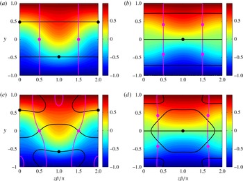
b) TG. The wall-normal inflection points are marked by the black curves while the spanwise inflection points are marked by magenta. The strongest wall-normal inflection points, having the maximum wall-normal shear, are indicated by the black circles and the strongest spanwise inflection points, having the maximum spanwise shear, by the magenta circles. For the even TG the wall-normal inflection points are near
 $y=\pm 0.5$
in between the vortices at
 $z\unicode[STIX]{x1D6FD}/\unicode[STIX]{x03C0}=0,1$
, respectively, whereas the spanwise inflection points are at the centre of the channel close to the cores of the vortices (
 $y=0,z\unicode[STIX]{x1D6FD}/\unicode[STIX]{x03C0}=0.5,1.5$
). For the odd TG the strongest wall-normal inflection point is at the centre of the channel
 $(y=0)$
in between the vortices
 $(z\unicode[STIX]{x1D6FD}/\unicode[STIX]{x03C0}=1)$
, whereas the spanwise inflection points are located on the sides of the channel close to the cores of the vortices (
 $y=\pm 0.5,z\unicode[STIX]{x1D6FD}/\unicode[STIX]{x03C0}=0.5,1.5$
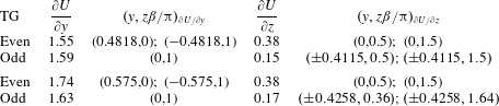
). The locations of the inflection points along with their strength (shear) are summarized in the top two rows of table 1. It can be seen that both types of TG generate wall-normal inflections with similar strength and that the even TG produces stronger spanwise inflections. The streamwise component of the modified base flow, taking into account the nonlinear interactions between the 4 TG modes, is presented in figure 1(c) and 1(d) for the even and odd TG, respectively. The locations of the inflection points along with their strength (shear) are summarized in the bottom two rows of table 1. It can be seen that the nonlinear modification has some effect on the streaks and changes the locations of the inflection points. Nevertheless, this effect can be considered small since qualitatively the streamwise component is similar to the one obtained using linear TG and the shift in the locations of the inflection points is relatively small. The nonlinear modification also enhances the strength of the inflection points and the most noticeable effect is on the wall-normal shear for the even TG. There is no effect on the spanwise shear for the even TG since the nonlinear modification of the streamwise velocity is antisymmetric with respect to
 $y=0$
and consequently the strongest spanwise inflection remains unchanged. The effect on the spanwise shear for the odd TG is small. To summarize, linear TG can be used as an adequate approximation for the calculation of the strongest inflection points for various combinations of
 $(\unicode[STIX]{x1D6FD},t)$
.
Streamwise modified base flow for
 $Re=1000$
,
 $E_{0}=10^{-4}$
,
 $\unicode[STIX]{x1D6FD}=1$
and
 $t=30$
. The wall-normal (black) and spanwise (magenta) inflection points contours are marked on the figures with the strongest inflections encircled. (a) Even, linear TG; (b) odd, linear TG; (c) even, nonlinear TG modification; (d) odd, nonlinear TG modification.

The shear and location of the strongest wall-normal and spanwise inflection points for even and odd TG,
 $Re=1000$
,
 $E_{0}=10^{-4}$
,
 $\unicode[STIX]{x1D6FD}=1$
and
 $t=30$
. The top two rows are for linear TG whereas the bottom two rows include the nonlinear TG modification.

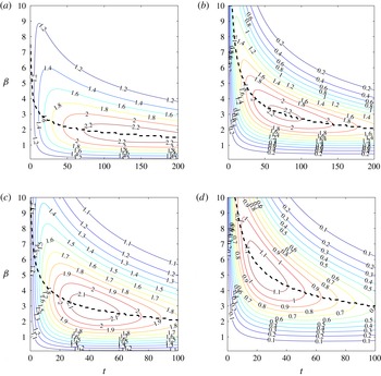
Maximal shear at the inflection points versus time and
 $\unicode[STIX]{x1D6FD}$
for linear TG,
 $Re=1000$
and
 $E_{0}=10^{-4}$
. (a) Even TG, maximal wall-normal inflection
 $|\unicode[STIX]{x2202}U/\unicode[STIX]{x2202}y|$
; (b) even TG, maximal spanwise inflection
 $|\unicode[STIX]{x2202}U/\unicode[STIX]{x2202}z|$
; (c) odd TG, maximal wall-normal inflection
 $|\unicode[STIX]{x2202}U/\unicode[STIX]{x2202}y|$
; (d) odd TG, maximal spanwise inflection
 $|\unicode[STIX]{x2202}U/\unicode[STIX]{x2202}z|$
. The strongest inflections versus time are given by the dashed lines.

The calculation of the strongest inflection points has been repeated for various wavenumbers and times (
 $\unicode[STIX]{x1D6FD},t$
). The shear at the strongest wall-normal and spanwise inflection points is presented in figure 2 for the even (2
a) and odd (2
b) TG,
 $Re=1000$
and
 $E_{0}=10^{-4}$
. It can be seen that the optimal wavenumber depends on time. For the even TG the maximal wall-normal inflection is obtained for
 $\unicode[STIX]{x1D6FD}=1.7$
, similarly to the optimal energy gain (Butler & Farrell Reference Butler and Farrell1992,
 $G_{max}(\unicode[STIX]{x1D6FD})$
). This is due to the fact that most of the energy is contained in the streamwise velocity, suggesting that maximum deviation of the streamwise velocity from the Couette profile is likely to produce the strongest wall-normal inflection as well as the largest energy growth. The optimal spanwise inflection is obtained at
 $\unicode[STIX]{x1D6FD}=3$
. This wavenumber corresponds approximately to an optimum of
 $\unicode[STIX]{x1D6FD}\sqrt{G_{max}(\unicode[STIX]{x1D6FD})}$
since for linear TG
 $\unicode[STIX]{x2202}U/\unicode[STIX]{x2202}z=-\unicode[STIX]{x1D6FD}u_{1}\sin (\unicode[STIX]{x1D6FD}z)$
and
 $u_{1}\sim \sqrt{G}$
. The optimal values for the odd TG are
 $\unicode[STIX]{x1D6FD}=2.8$
and
 $\unicode[STIX]{x1D6FD}=5.2$
for the wall-normal and spanwise inflections, respectively. It should be noted that in contrast to the maximal energy growth, which is much larger for the even TG, the strength of the inflection points generated by the even and odd TG is comparable and there exists a region (e.g.
 $t\leqslant 30$
) where the odd TG generates inflection points stronger than the ones generated by the even TG. Nevertheless, the spanwise inflections generated by the even TG are always stronger than the ones generated by the odd TG.
Next, the above calculation of the strongest inflection points has been repeated including the nonlinear TG modification. The strongest inflection points, together with the optimal wavenumbers and times when they are obtained are summarized in table 2 in which the top two rows correspond to linear TG, whereas the bottom two rows to TG including nonlinear modification. It can be seen that the nonlinear TG modification affects the wall-normal inflections, changing the optimal parameters and enhancing the maximal wall-normal shear. Nevertheless, its influence on the spanwise shear is negligible. It should be noted that the even TG spans over longer times compared to the odd TG (note the different time scales in figure 2). This is best understood by considering very long times when only one least stable mode is left in the TG. The ratio between the decay rates (see (A 1)) of the least stable even and odd modes is
 $\unicode[STIX]{x1D714}_{sq_{e}}/\unicode[STIX]{x1D714}_{sq_{o}}=(0.25+(\unicode[STIX]{x1D6FD}/\unicode[STIX]{x03C0})^{2})/(1+(\unicode[STIX]{x1D6FD}/\unicode[STIX]{x03C0})^{2})$
, which varies between 0.25 for small
 $\unicode[STIX]{x1D6FD}$
to
 $1$
as
 $\unicode[STIX]{x1D6FD}\rightarrow \infty$
. Consequently, the inflection points generated by the even TG remain in the modified base flow for longer times, making the even TG a better candidate for possible instability.
The shear at the strongest wall-normal and spanwise inflection points and the optimal wavenumbers
 $\unicode[STIX]{x1D6FD}$
and times
 $t$
when it is attained for even and odd TG,
 $Re=1000$
and
 $E_{0}=10^{-4}$
. The top two rows are for linear TG whereas the bottom two rows include the nonlinear TG modification.

3.2 Secondary stability analysis
To verify that the strongest secondary instability is indeed associated with the strongest inflection points, a 3-D stability analysis of the two-dimensional (2-D) modified base flow is performed. A Floquet decomposition is utilized in the spanwise direction, with
 $M_{z}=5$
Fourier modes and
 $N_{y}=100$
Chebyshev modes over the 2-D domain
 $z\unicode[STIX]{x1D6FD}/\unicode[STIX]{x03C0}=[-1,1];y=[-1,1]$
. There are two types of modes – varicose and sinuous. Usually the varicose modes are associated with wall-normal inflections whereas the sinuous modes are associated with spanwise inflections. However, there may exist other combinations, such as varicose modes associated with spanwise inflections or sinuous modes associated with wall-normal inflections, depending on the relative strength of the spanwise and wall-normal inflection points. The analysis is based only on the streamwise component as the cross-stream components are an order of magnitude smaller than the streamwise component (as is evident from (A 3)), with the time being ‘frozen’ and used as a parameter. The nonlinear TG modification is included in the modified base flow since in our previous work (Karp & Cohen Reference Karp and Cohen2014) it was found to be influential for initial energies of order
 $O(10^{-4})$
and
 $Re=1000$
. An additional parameter required for the stability analysis is the streamwise wavenumber of the secondary disturbance,
 $\unicode[STIX]{x1D6FC}$
.
The 3-D stability analysis for even and odd TG,
 $Re=1000$
and
 $E_{0}=10^{-4}$
has been performed in the parameter space
 $(\unicode[STIX]{x1D6FC},\unicode[STIX]{x1D6FD},t)$
. The combinations yielding the highest growth rate are given in table 3 for the varicose and sinuous modes, together with the values of
 $T_{y}/(2E_{d}),T_{z}/(2E_{d})$
and
 $D/(2E_{d})$
. It can be seen that the optimal spanwise wavenumbers are different compared to the ones maximizing the energy gain (
 $\unicode[STIX]{x1D6FD}=1.67$
, 2.8 for the even/odd TG, respectively). The most dangerous secondary disturbance is sinuous and the even TG is more unstable than the odd TG. For both sinuous disturbances the wavenumbers are very similar and
 $\unicode[STIX]{x1D6FC}\approx 0.5\unicode[STIX]{x1D6FD}$
. Examining the growth rate components
 $(T_{y},T_{z},D)$
it is evident that the sinuous modes, as well as the varicose mode of the even TG, are associated with spanwise inflection points while the varicose mode of the odd TG is associated with wall-normal inflections.
The optimal parameters yielding the maximal growth rate for
 $Re=1000$
and
 $E_{0}=10^{-4}$
for even and odd TG including nonlinear modifications based on a 3-D analysis of a 2-D base flow.

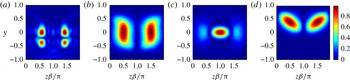
The streamwise magnitude of the above four secondary disturbances is presented in figure 3. The even-varicose mode (figure 3
a) is maximal near the locations of the strongest spanwise inflections. The combination of a varicose mode and spanwise inflections is somewhat surprising. Therefore this disturbance is compared with a sinuous disturbance calculated for the same parameters (
 $\unicode[STIX]{x1D6FC}=2.5,\unicode[STIX]{x1D6FD}=2.1$
and
 $t=81$
). It is found that for these parameters, which maximize the varicose instability, the sinuous disturbance is more unstable than the varicose disturbance. This implies that the varicose disturbance should not be treated as a separate route to transition, as it is completely masked by the sinuous disturbance. Therefore, only three instability mechanisms remain relevant, even sinuous, odd varicose and odd sinuous. The sinuous disturbances (figure 3
b,d) are maximal near the locations of the strongest spanwise inflections. The mode associated with the even TG spans through the entire channel (figure 3
b) whereas the one associated with the odd TG is concentrated in the upper half of the channel (figure 3
d) (the latter mode has a complex conjugate mode concentrated in the lower half of the channel). As the spanwise shear is stronger for the even TG, the growth rate is also higher for this case. The physics behind both these modes is very similar as their instability is triggered via the spanwise inflection points between a single pair of vortices. This type of instability has been investigated by Waleffe (Reference Waleffe1995) and Reddy et al. (Reference Reddy, Schmid, Baggett and Henningson1998). The odd-varicose mode (figure 3
c) is maximal near the location of the strongest wall-normal inflection. This type of disturbance has been investigated in our previous work (Karp & Cohen Reference Karp and Cohen2014).
Magnitude of the streamwise component of the secondary disturbance corresponding to the parameters in table 3, obtained by stability analysis of a 2-D base flow, including the nonlinear TG modification for
 $Re=1000$
and
 $E_{0}=10^{-4}$
. (a) Varicose, even TG; (b) sinuous, even TG; (c) varicose, odd TG; (d) sinuous, odd TG.

Comparing the most unstable secondary disturbances to the inflection point strength in table 2 several interesting observations can be made: (i) although the wall-normal inflection points are stronger than the spanwise inflection points, the latter trigger instability more efficiently, since the sinuous modes are more unstable than the varicose modes. A possible reason for the dominance of the spanwise inflections is the absence of walls in the spanwise direction; (ii) the even TG generates a stronger wall-normal inflection point compared to the odd TG. Nevertheless, only the odd TG has an instability associated with a wall-normal inflection. This is attributed to the location of the wall-normal inflection points associated with the even TG, which varies with time and located closer to the wall; and (iii) the optimal spanwise wavenumbers which maximize the secondary instability are not exactly the same as the ones maximizing the strength of the inflection points. The differences between them result from the two-dimensionality of the modified base flow which is not taken into account in the inflection point strength study. The effect of the two-dimensionality of the modified base flow can be evaluated by looking at the dependence of the growth rate components (
 $T_{y},T_{z},D$
) on
 $\unicode[STIX]{x1D6FD}$
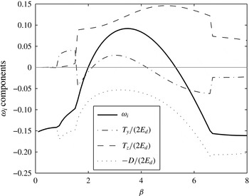
. These are shown in figure 4 for the odd-sinuous mode (
 $Re=1000,E_{0}=10^{-4},\unicode[STIX]{x1D6FC}=1.5$
and
 $t=36$
). It can be seen that indeed the
 $T_{z}$
component, associated with the spanwise shear, is stronger at
 $\unicode[STIX]{x1D6FD}=5$
(corresponding to the strongest spanwise inflections). However, the effect of
 $T_{y}$
, associated with the wall-normal shear, and the dissipation
 $D$
results in a shift of the optimal spanwise wavenumber to
 $\unicode[STIX]{x1D6FD}=3.5$
. Thus, the difference in the spanwise wavenumber is due to 2-D effects and not due to a different mechanism. For the other secondary modes similar effects are observed (not shown).
To understand the reasons for some of these observations stability analysis of one-dimensional (1-D) velocity profiles containing the strongest inflection points (wall-normal or spanwise, in accordance with the inflection point direction) can be performed. This analysis is carried out in appendix C, leading to the following conclusions: (i) the highest growth rate corresponds to the spanwise 1-D profiles of the even and odd TG, suggesting that the spanwise inflections are more dominant than the wall-normal inflections; and (ii) for the wall-normal 1-D profiles, the odd TG is much more unstable than the even TG, suggesting that the wall-normal inflections of the even TG are not capable of introducing a significant instability. It can be seen that analysis of the 1-D velocity profiles predicts the tendencies observed in the full analysis of the 2-D flow. Nevertheless, the 1-D stability analysis is clearly insufficient to find the optimal parameters for the instability and the growth rate.
Growth rate components versus
 $\unicode[STIX]{x1D6FD}$
for the odd TG with nonlinear modification, sinuous disturbance,
 $Re=1000,E_{0}=10^{-4},\unicode[STIX]{x1D6FC}=1.5$
and
 $t=36$
.

3.3 Effect of initial energy, TG nonlinearity and Reynolds number
In this section the effect of initial energy, TG nonlinearity and
 $Re$
on the three most dangerous secondary disturbances identified above is presented. The most dangerous secondary disturbances have been obtained above including the nonlinear TG modification in the modified base flow. Here, the effect of neglecting the nonlinear TG modification is examined by excluding
 $u_{2}$
. As the initial energy is increased, more nonlinear TG effects come into play and many other secondary modes may become unstable. However, our analytical model for the TG becomes less valid for higher initial energies and we are interested in working with the smallest initial energy allowing instability. Thus, we are particularly interested in the effect of lowering the initial energy. To isolate the effect of the initial energy, the growth rate of each of the three eigenmodes is calculated while keeping
 $(\unicode[STIX]{x1D6FC},\unicode[STIX]{x1D6FD})$
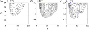
constant. The growth rates for these three eigenmodes for various times and initial energies are presented in figure 5, where only positive growth rates are shown. It can be seen that the time when the growth rate is optimal is almost constant. This is in accordance with the effect of
 $E_{0}$
on the inflection points. According to linear TG the locations of the optimal inflection points do not change and their strength (shear) is proportional to
 $\sqrt{E_{0}}$
(see (A 3) and (A 4)). The most significant change in the growth rate is for the even TG (figure 5
a), whereas for the odd TG the changes are similar for both modes (figure 5
b,c). The threshold energy for instability varies between
 $4\times 10^{-5}$
for the even-sinuous case to
 $7\times 10^{-5}$
for the odd-varicose case. Nevertheless, the optimal parameters (
 $\unicode[STIX]{x1D6FC},\unicode[STIX]{x1D6FD}$
) may vary with
 $E_{0}$
, so lower thresholds for instability may be found. It should be noted that Reddy et al. (Reference Reddy, Schmid, Baggett and Henningson1998) have calculated thresholds for instability based on a numerical TG representation with many modes, albeit only for the even TG.
Effect of initial energy on the growth rate of the optimal secondary disturbances in table 3, for
 $Re=1000$
and various times. The growth rate is obtained by stability analysis of a 2-D base flow, including nonlinear TG modifications. Maximal growth rate curves are indicated by the dashed lines and only positive growth rates are shown. (a) Sinuous, even TG,
 $\unicode[STIX]{x1D6FC}=1.8$
,
 $\unicode[STIX]{x1D6FD}=3.6$
; (b) varicose, odd TG,
 $\unicode[STIX]{x1D6FC}=1.2$
,
 $\unicode[STIX]{x1D6FD}=1.6$
; (c) sinuous, odd TG,
 $\unicode[STIX]{x1D6FC}=1.5$
,
 $\unicode[STIX]{x1D6FD}=3.5$
.

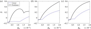
The effect of TG nonlinearity is shown in figure 6, where the growth rates versus initial energy for linear TG (dashed) and including nonlinear TG modification (solid) are presented for the three eigenmodes, while keeping
 $(\unicode[STIX]{x1D6FC},\unicode[STIX]{x1D6FD},t)$
constant. It can be seen that for values of initial energy lower than
 $E_{0}\approx 3\times 10^{-5}$
the TG nonlinearity has a minor effect on the growth rate. For higher values of the initial energy the growth rate including TG nonlinearity is considerably larger than the one associated with the linear TG. The linear TG becomes unstable only for initial energies of
 $E_{0}\approx 1.5\times 10^{-4}$
, for which the TG nonlinearity is important. It should be noted that even for initial energies of
 $O(10^{-5})$
the nonlinear TG modification has a minor effect, expressed by the small deviations between the curves.
Effect of TG nonlinearity on the growth rate of the optimal secondary disturbances in table 3 for
 $Re=1000$
. The growth rate (
 $\unicode[STIX]{x1D714}_{i}$
) as a function of initial energy (
 $E_{0}$
) is obtained by stability analysis of a 2-D base flow. (a) Sinuous, even TG,
 $\unicode[STIX]{x1D6FC}=1.8$
,
 $\unicode[STIX]{x1D6FD}=3.6$
,
 $t=61$
; (b) varicose, odd TG,
 $\unicode[STIX]{x1D6FC}=1.2$
,
 $\unicode[STIX]{x1D6FD}=1.6$
,
 $t=43$
; (c) sinuous, odd TG,
 $\unicode[STIX]{x1D6FC}=1.5$
,
 $\unicode[STIX]{x1D6FD}=3.5$
,
 $t=36$
.

Lowering the Reynolds number has several effects on the eigenvalues. The TG time scale is shortened (A 1), the streamwise velocity of the modified base flow is lowered (A 3) and the effect of dissipation (
 $D$
) on the growth rate of the secondary disturbance becomes more noticeable (2.16a,b
). To isolate each of these effects as
 $Re$
is lowered, the growth rate of each of the three eigenmodes is calculated while keeping
 $(\unicode[STIX]{x1D6FC},\unicode[STIX]{x1D6FD})$
constant and changing the initial energy according to the relation
 $E_{0}=10^{-4}(1000/Re)^{2}$
. Changing
 $E_{0}$
allows keeping the strength of the inflectional points fairly constant (they are not strictly constant as nonlinear TG modifications are included). It should be noted that the dictated increase in initial energy as
 $Re$
is lowered results in higher amplitudes of the TG which result in more significant nonlinear TG interactions, not taken into account in our simplified model. Therefore, the growth rates should be interpreted as leading-order results with respect to
 $Re$
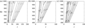
. The growth rates for the three eigenmodes for various times and
 $Re$
are presented in figure 7, where only positive growth rates are shown. It can be seen that the time when the growth rate is optimal is linearly proportional to
 $Re$
although the analysis includes nonlinear TG modifications. Thus, the TG time scale is linearly proportional to
 $Re$
even when the TG includes nonlinear modifications. As
 $Re$
is lowered, the optimal growth rate reduces due to the higher dissipation. The decrease in the optimal growth rate as
 $Re$
is lowered is similar for all three modes. This suggests that the threshold energy for instability should change with a power
 $n$
, higher than
 $-2$
which is used for
 $E_{0}$
above (i.e.
 $E_{0}\sim Re^{n}$
,
 $n>-2$
). Nevertheless, it can be seen that the growth rate of each one of the three modes continues smoothly to lower
 $Re$
with the window of instability, i.e. the time range when each of the modes is unstable, shrinking linearly with
 $Re$
. For transition to occur we would like to choose the most unstable eigenmode which has the largest window of instability. This mode is associated with the even TG as it generates spanwise inflection points for longer times.
Effect of
 $Re$
on the growth rate of the optimal secondary disturbances in table 3, for various times. The growth rate is obtained by stability analysis of a 2-D base flow, including nonlinear TG modifications. Maximal growth rate curves are indicated by the dashed lines and only positive growth rates are shown. The initial energy used in the calculation is given by
 $E_{0}=10^{-4}(1000/Re)^{2}$
. (a) Sinuous, even TG,
 $\unicode[STIX]{x1D6FC}=1.8$
,
 $\unicode[STIX]{x1D6FD}=3.6$
; (b) varicose, odd TG,
 $\unicode[STIX]{x1D6FC}=1.2$
,
 $\unicode[STIX]{x1D6FD}=1.6$
; (c) sinuous, odd TG,
 $\unicode[STIX]{x1D6FC}=1.5$
,
 $\unicode[STIX]{x1D6FD}=3.5$
.

3.4 Stability for temporally slowly evolving flow and comparison with DNS
In the previous sections the stability properties of PCF modified by TG have been investigated and the most dangerous disturbances have been identified. To verify our stability analysis and further investigate the mechanism of instability we have simulated the evolution of the disturbances in DNS. Our model assumes a separation of time scales between the slowly varying TG and the rapidly growing secondary disturbance. The TG is initially algebraic and becomes slowly varying only at some finite time. Accordingly, to test our model, the simulation should not be initiated at
 $t=0$
but rather at a time when the TG is already slowly varying and a separation of time scales exists. The variation of the TG is estimated from the linear energy gain by calculation of the local TG growth rate:
 $$\begin{eqnarray}\unicode[STIX]{x1D714}_{TG}=\frac{\unicode[STIX]{x2202}}{\unicode[STIX]{x2202}t}\left(\ln \sqrt{G}\right)=\frac{1}{2G}\frac{\unicode[STIX]{x2202}G}{\unicode[STIX]{x2202}t}.\end{eqnarray}$$
The local TG growth rate has been compared with the growth rate of the secondary eigenmode for several times and the initial time
 $t_{0}$
for the simulation has been chosen to ensure that
 $\unicode[STIX]{x1D714}_{i}\gg |\unicode[STIX]{x1D714}_{TG}|$
. Since nonlinear TG effects are non-negligible they have been included in the initial conditions for the DNS. To summarize, the DNS is initiated with the analytical expressions (including linear TG and its nonlinear modification) at time
 $t_{0}$
and the corresponding secondary disturbance. Three scenarios have been investigated: even TG with a sinuous disturbance, odd TG with a varicose disturbance and odd TG with a sinuous disturbance. The initial times and growth rates for these three cases are summarized in table 4. The transition scenario for each of the cases is analysed separately in the following sections. The amplitude of the secondary disturbance has been chosen so that the fraction of energy in the secondary disturbance is
 $1\,\%$
of the initial TG energy (e.g. for
 $E_{0}=10^{-4}$
the secondary disturbance adds the energy
 $\unicode[STIX]{x1D6E5}E=10^{-6}$
to the TG at time
 $t_{0}$
).
The DNS results are compared for each scenario to the corresponding analytical expressions obtained by using the multiple time scales method. To highlight the advantage of the multiple time scales method over the frozen flow analysis, i.e. assuming the secondary disturbance has constant growth rate and eigenfunction, a direct comparison between the two analytical methods has been performed, as detailed in appendix D. It is shown that the multiple time scales better predicts the DNS results.
Summary of the parameters used in the scenarios tested in the DNS for
 $Re=1000$
. The initial time
 $t_{0}$
is chosen to ensure
 $\unicode[STIX]{x1D714}_{i}\gg |\unicode[STIX]{x1D714}_{TG}|$
.

3.4.1 Even TG, sinuous instability
For this scenario and initial energy
 $E_{0}=10^{-4}$
a very significant growth rate has been obtained (table 3 row 2) and the instability persists for very long times. Therefore, before testing this scenario, the initial energy has been lowered to
 $E_{0}=0.5\times 10^{-4}$
. The wavenumbers
 $(\unicode[STIX]{x1D6FC},\unicode[STIX]{x1D6FD})$
have been chosen to obtain an eigenmode similar to the optimal one (obtained for higher energy). It should be emphasized that the physical mechanism of transition for both scenarios – the one presented below and the one which can be obtained for
 $E_{0}=10^{-4},\unicode[STIX]{x1D6FD}=3.6$
and
 $\unicode[STIX]{x1D6FC}=1.8$
– is the same. The effect of changing the wavenumbers is small as seen by comparing the growth rate in table 4 row 1 to the one encircled in figure 5(a) (in both cases
 $\unicode[STIX]{x1D714}_{i}(t_{0})\approx 0.1$
). The DNS initiated at
 $t_{0}=50$
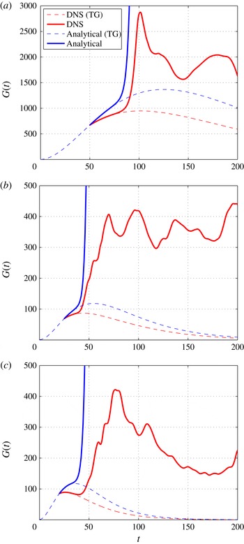
yields transition. The energy growth for this scenario is presented in figure 8(a). The energy during transition is indicated by the solid red line along with the unperturbed TG scenario (without a secondary disturbance) indicated by the red dashed line. The analytical approximation of the transition scenario using the multiple scales method is given by the solid blue line and the analytical curve for the unperturbed TG is indicated by the blue dashed line. The rapid transition occurring at
 $t\approx 90$
justifies the multiple time scales approach and a very good agreement is observed between the DNS and the analytical approximation. However, a significant difference in the unperturbed TG scenarios can be seen. This difference results from higher-order nonlinear TG interactions between the four modes which have not been accounted for in the derivation (i.e.
 $O(\unicode[STIX]{x1D700}^{3})$
). However, this difference has only a marginal effect on the evolution of the vortical structures corresponding to the secondary instability, as discussed below. The good agreement between DNS and theory indicates that the additional nonlinear TG interactions do not influence the transition scenario significantly.
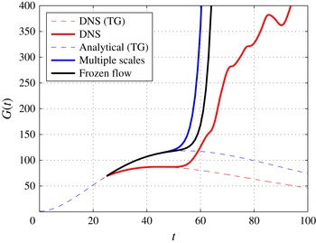
Energy growth during transition; the parameters are indicated in table 4. Comparison between DNS (red) and analytical (blue) approximation. Unperturbed TG scenarios are indicated by the dashed lines. (a) Sinuous, even TG; (b) varicose, odd TG; (c) sinuous, odd TG.

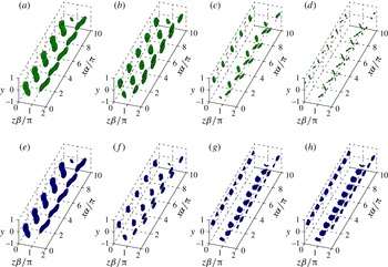
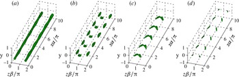
The evolution of the vortical structures during transition is shown in figure 9. To identify the vortical structure,
 $Q$
, the second invariant of the velocity gradient tensor, is used (
 $Q=-0.5\unicode[STIX]{x2202}u_{i}/\unicode[STIX]{x2202}x_{j}\cdot \unicode[STIX]{x2202}u_{j}/\unicode[STIX]{x2202}x_{i}$
(Hunt, Wray & Moin Reference Hunt, Wray and Moin1988)). During the evolution the vortices split antisymmetrically due to the sinuous disturbance (figure 9
a). Later on, they split again (figure 9
b). Just before transition, alternating vortices are formed and intensified close to the walls (figure 9
c,d) and shortly after the flow transitions to turbulence. This transition is dominated by spanwise inflections and is in accordance with the previous studies of Waleffe (Reference Waleffe1997) and Reddy et al. (Reference Reddy, Schmid, Baggett and Henningson1998). The structures obtained analytically using multiple scales are shown in figure 9(e–h) for the same times and values of
 $Q$
as in figure 9(a–d). It can be seen that there is a very good agreement between the analytical predictions and the results from DNS at the initial transition stages (figure 9
a,b versus 9
e,f). The final stages (figure 9
c,d versus 9
g,h) are not captured well due to additional nonlinear interactions (
 $O(\unicode[STIX]{x1D6FF}^{2})$
) which have not been taken into account. The good agreement during the initial evolution strengthens our conclusion that the additional nonlinear TG interactions (
 $O(\unicode[STIX]{x1D700}^{3})$
) are not essential to follow the transition process.
Structures during transition for even TG and a sinuous secondary disturbance; the parameters are indicated in table 4 row 1. Comparison between DNS (top row) and analytical (bottom row) approximation. All isosurfaces correspond to
 $Q/Q_{max}=0.7$
. (a,e)
 $t=50$
; (b,f)
 $t=75$
; (c,g)
 $t=85$
; (d,h)
 $t=90$
.

3.4.2 Odd TG, varicose instability
For this scenario and initial energy
 $E_{0}=10^{-4}$
the optimal growth rate has not been sufficiently high to ensure separation of time scales with the TG (table 3 row 3). Therefore, before testing this scenario the initial energy has been increased to
 $E_{0}=2\times 10^{-4}$
. The wavenumbers
 $(\unicode[STIX]{x1D6FC},\unicode[STIX]{x1D6FD})$
have been chosen to obtain an eigenmode similar to the optimal one (obtained for the lower energy). As mentioned before, the physical mechanism of transition is the same between the scenario presented below and the one which can be obtained for
 $E_{0}=10^{-4},\unicode[STIX]{x1D6FD}=1.6$
and
 $\unicode[STIX]{x1D6FC}=1.2$
. The effect of changing the wavenumbers is small as seen by comparing the growth rate in table 4 row 2 to the one encircled in figure 5(b) (in both cases
 $\unicode[STIX]{x1D714}_{i}(t_{0})\approx 0.15$
). The DNS initiated at
 $t_{0}=25$
yields transition. The energy growth for this scenario is presented in figure 8(b). It can be seen that there is a very good agreement between the analytical predictions and the DNS and that the transition occurs rapidly around
 $t\approx 45$
. It should be noted that while for the even TG (figure 8
a) a significant gain is achieved during the TG stage (
 $G\approx 1000$
), for the odd TG (figure 8
b) the gain is one order of magnitude lower (
 $G\approx 100$
). Nevertheless, the energy level after transition is similar (note that
 $E_{0}$
in the even scenario is four times smaller than that of the odd scenario, so that a level of 1600 in figure 8(a) corresponds to a level of 400 in figure 8
b). This further exemplifies that maximal energy gain is not essential for transition.
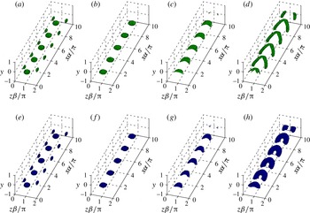
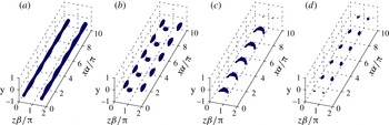
Structures during transition for odd TG and a varicose secondary disturbance; the parameters are indicated in table 4 row 2. Comparison between DNS (top row) and analytical (bottom row) approximation. Only the lower half of the domain is shown since the structures evolve symmetrically with respect to the
 $y$
axis. (a,e)
 $t=25$
,
 $Q/Q_{max}=0.5$
; (b,f)
 $t=30$
,
 $Q/Q_{max}=0.5$
; (c,g)
 $t=35$
,
 $Q/Q_{max}=0.5$
; (d,h)
 $t=40$
,
 $Q/Q_{max}=0.15$
.

The structures during transition are shown in figure 10. Only the lower half of the domain is shown since the structures evolve symmetrically with respect to the
 $y$
axis (for each structure moving downstream in the top half-domain there is a structure moving in the opposite direction in the bottom half-domain). The vortices experience symmetric modulations (figure 10
a). The spanwise vortical segments at the centre of the channel are intensified by
 $t=30$
(figure 10
b). Later they join with the streamwise vortical elements situated beneath them. Consequently, a packet of hairpins is formed (
 $t=35$
, figure 10
c). The packet further intensifies and the hairpin ‘heads’ become more localized having a shape of loops (
 $t=40$
, figure 10
d). Shortly afterwards the flow becomes turbulent. This transition is dominated by a wall-normal inflection at the centre of the channel. The structures obtained analytically using multiple scales are shown in figure 10(e–h). It can be seen that there is a very good agreement between the analytical predictions and the results from DNS. The evolution of the vortical structures in the above scenario is very similar to the mechanism of generation of a packet of hairpins proposed in the model by Cohen, Karp & Mehta (Reference Cohen, Karp and Mehta2014). Their model consists of three basic flow elements: pure shear, CVP and a wavy spanwise vortex secondary disturbance. The mechanism for the formation of a packet of hairpins is through streamwise undulations of the CVP which are enhanced due to a wall-normal inflectional instability.
3.4.3 Odd TG, sinuous instability
For this scenario and initial energy
 $E_{0}=10^{-4}$
the optimal growth rate has not been high enough to ensure separation of time scales with the TG (table 3 row 4). Therefore, before testing this scenario the initial energy has been increased to
 $E_{0}=2\times 10^{-4}$
. The wavenumbers
 $(\unicode[STIX]{x1D6FC},\unicode[STIX]{x1D6FD})$
have been chosen to obtain an eigenmode similar to the optimal one (obtained for the lower energy). As mentioned before, the physical mechanism of transition is the same between the scenario presented below and the one which can be obtained for
 $E_{0}=10^{-4},\unicode[STIX]{x1D6FD}=3.5$
and
 $\unicode[STIX]{x1D6FC}=1.5$
. The effect of changing the wavenumbers is small as seen by comparing the growth rate in table 4 row 3 to the one encircled in figure 5(c) (in both cases
 $\unicode[STIX]{x1D714}_{i}(t_{0})\approx 0.17$
). The DNS initiated at
 $t_{0}=20$
yields transition. The energy growth for this scenario is presented in figure 8(c). It can be seen that there is a good agreement between the analytical predictions and the DNS. The gain during the TG phase is similar to the one observed for the varicose mode (figure 8
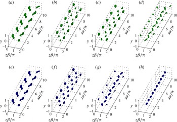
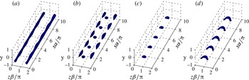
b) and the transition (in DNS) is less rapid compared to the previous two scenarios. The structures during transition are shown in figure 11. The transition stages are similar to the ones described for sinuous instability of the even TG since the disturbance is concentrated at the top half of the channel and its physics are based on the top two vortices. The vortices split antisymmetrically (figure 11
a), followed by additional splitting (figure 11
b). Finally alternating vortices are formed at the centre of the channel and close to the walls (figure 11
c,d) and shortly after the flow transitions to turbulence. This transition is dominated by spanwise inflections. The structures obtained analytically using multiple scales are shown in figure 11(e–h). It can be seen that there is a very good agreement between the analytical predictions and the results from DNS, except the last stage (figure 11
d,h) just prior to transition.
Structures during transition for odd TG and a sinuous secondary disturbance; the parameters are indicated in table 4 row 3. Comparison between DNS (top row) and analytical (bottom row) approximation. All isosurfaces correspond to
 $Q/Q_{max}=0.7$
. (a,e)
 $t=20$
; (b,f)
 $t=30$
; (c,g)
 $t=35$
; (d,h)
 $t=40$
.

4 Concluding remarks
Since the discovery of the linear TG phenomenon, corresponding to streamwise independent vortices, most of the research has concentrated on a single CVP (even TG) and spanwise wavenumbers which maximize the energy growth (e.g. Lundbladh et al. Reference Lundbladh, Henningson, Reddy and Hussaini1994; Waleffe Reference Waleffe1995, Reference Waleffe1997; Reddy et al. Reference Reddy, Schmid, Baggett and Henningson1998). This choice relies on the assumption that maximal energy growth ensures maximal secondary instability, which has been shown to be inaccurate in the current work. Consequently, a thorough investigation of the effect of various parameters, especially the spanwise wavenumber, has been performed and both TG kinds (even/odd) have been compared. This enables us to unambiguously conclude which secondary instability is the dominant one and under what conditions. In the previous studies the modified base flow has been assumed either steady (Waleffe Reference Waleffe1995, Reference Waleffe1997) or slowly varying, with the time being used as a parameter (Reddy et al. Reference Reddy, Schmid, Baggett and Henningson1998; Karp & Cohen Reference Karp and Cohen2014). In the current work the effect of the temporal variation of the modified base flow on the evolution of the secondary disturbance is taken into account, using the multiple time scales method. This allows a quantitative comparison between the analytical expressions and DNS, which has not been possible in our previous work (Karp & Cohen Reference Karp and Cohen2014).
The secondary stability of TG in Couette flow has been studied thoroughly and the parameters maximizing the growth rate have been identified. These optimal parameters are not associated with spanwise wavenumbers which maximize the energy gain but the ones which generate the strongest inflection points, i.e. those having maximal shear. Parametric investigation reveals three types of secondary disturbances: (i) sinuous instability of the even TG, associated with the generation of spanwise inflections; (ii) varicose instability of the odd TG, associated with the generation of a wall-normal inflection point at the centre of the channel; and (iii) sinuous instability of the odd TG, associated with the generation of spanwise inflections by the top (or bottom) two vortices. Comparison between the secondary stability analysis of the 2-D base flow with a simple stability analysis of the 1-D profiles containing the strongest inflection points reveals that the latter correctly predicts the following two tendencies: (i) spanwise inflections are more dominant than wall-normal inflections; and (ii) the wall-normal inflections of the even TG are not capable of introducing a significant instability.
The initial energy has been found to be most influential on the sinuous disturbance associated with the even TG. The time when the growth rate is optimal has been found to depend weakly on the initial energy for all three instability modes. This is attributed to the behaviour of the inflection points, which are maximized approximately at the same times for various initial energies. The TG nonlinearity is important for the secondary instability as the linear TG becomes unstable only for initial energies where the TG nonlinearity is non-negligible. The effect of lowering
 $Re$
(while adjusting
 $E_{0}\sim Re^{-2}$
) is a decrease in the optimal growth rates of the secondary disturbances due to higher dissipation. The optimal growth rates and their time windows of instability are linearly increasing with
 $Re$
for all three instability modes. The secondary disturbance which has the highest growth rate, as well as the biggest time window of instability, is the sinuous mode associated with the even TG as it generates stronger spanwise inflection points for longer times.
The routes to turbulence for each of the three modes have been obtained using DNS initiated by the analytical expressions. The mechanism of transition for the sinuous disturbances is through antisymmetric breakdown of a pair of vortices (both even and odd TG) and for the varicose disturbance through a packet of hairpins (odd TG). The gain just before transition is one order of magnitude higher for the even TG compared to the odd TG, showing that the maximal energy gain criteria is not essential for transition. The DNS results have been compared with analytical predictions based on the multiple scales method, taking advantage of the time scales separation associated with the TG stage and the evolution of the secondary instability. Consequently, a very good agreement between the theoretical model and DNS has been obtained, except for the last stage just prior to transition. This demonstrates that our representation of the TG by four modes and their nonlinear interactions, together with a linear secondary instability and the use of time scales separation, are sufficient for understanding the main stages of subcritical transition. It should be noted that the time of transition depends on the amplitude of the secondary disturbance. As this amplitude is lowered the transition is delayed (or may not occur at all). This may lead to bigger differences between the analytical model and the DNS, since our approximation is better for shorter times.
It has been shown that the strongest inflection points are correlated with the maximal growth of secondary instabilities. Nevertheless, it should be noted that generalization of this statement to other flows requires further investigation. For instance, for a boundary layer with cross-flow, Wassermann & Kloker (Reference Wassermann and Kloker2002) found that the onset of secondary instability is more connected to the maximal localized mean flow deceleration caused by the vortices, than to the strength of the shear layer at the updraught vortex side. On a more general level, identification of sinuous instabilities as the most dangerous ones allegedly contradicts results of some transitional experiments in channel flow (e.g. Philip, Svizher & Cohen Reference Philip, Svizher and Cohen2007; Philip, Karp & Cohen Reference Philip, Karp and Cohen2016) and pipe flow (e.g. Cohen et al. Reference Cohen, Karp and Mehta2014), where varicose instabilities have been observed, leading to the formation of packets of hairpins. This contradiction can be explained by addressing the role of the wall. In the above model for TG, the CVP and its associated streaks span through the entire channel height and the wall-normal inflection point is formed close to the wall. Consequently, the secondary disturbance, triggering instability through this inflection point, is confined by the wall. Alternatively, in the experiments the streaks are concentrated in a certain region, smaller than the height (diameter) of the channel (pipe). Therefore, the remote walls in this case allow the secondary disturbances, associated with the wall-normal inflections, to achieve significant growth rates which often surpass the growth rates of the sinuous modes.
Acknowledgements
This research was supported by the Israeli Science Foundation under grant no. 1394/11. M.K. would like to thank the Israeli Ministry of Science, Technology and Space for their travel support grant.
Appendix A. Analytical model for TG
This appendix presents the analytical model for the TG based on four modes. The full derivation is presented in Karp & Cohen (Reference Karp and Cohen2014) and only essential final expressions required for the present work are given here, for completeness. For the streamwise independent case the Orr–Sommerfeld and Squire equations (
 $O(\unicode[STIX]{x1D700})$
) can be solved analytically. In that case
 $\unicode[STIX]{x1D714}$
is purely imaginary and negative, corresponding to pure decay of the modes. The expression for
 $\unicode[STIX]{x1D714}$
is:
 $$\begin{eqnarray}\unicode[STIX]{x1D714}_{k}=-\frac{\text{i}}{Re}(p_{k}^{2}+\unicode[STIX]{x1D6FD}^{2}),\end{eqnarray}$$
where the equations for
 $p_{k}(k=os_{e},os_{o},sq_{e},sq_{o})$
are given respectively by
 $$\begin{eqnarray}\unicode[STIX]{x1D6FD}\tanh \unicode[STIX]{x1D6FD}+p_{os_{e}}\tan p_{os_{e}}=0;\quad \unicode[STIX]{x1D6FD}\coth \unicode[STIX]{x1D6FD}-p_{os_{o}}\cot p_{os_{o}}=0,\end{eqnarray}$$
 $$\begin{eqnarray}p_{sq_{e}}=\unicode[STIX]{x03C0}/2,3\unicode[STIX]{x03C0}/2;\quad p_{sq_{o}}=\unicode[STIX]{x03C0},2\unicode[STIX]{x03C0},\end{eqnarray}$$
for the Orr–Sommerfeld (
 $OS$
) and Squire (
 $Sq$
), even (
 $e$
) and odd (
 $o$
) modes. Taking a combination of four modes the analytical expression for the velocity field is
 $$\begin{eqnarray}\displaystyle u_{1}(t,y,z) & = & \displaystyle a_{0}\unicode[STIX]{x1D6FA}Re\left[a_{1}F_{sq_{1}}(y)\text{e}^{-\text{i}\unicode[STIX]{x1D714}_{sq_{1}}t}+F_{os_{1}}(y)\text{e}^{-\text{i}\unicode[STIX]{x1D714}_{os_{1}}t}\right.\nonumber\\ \displaystyle & & \displaystyle +\left.a_{2}F_{sq_{2}}(y)\text{e}^{-\text{i}\unicode[STIX]{x1D714}_{sq_{2}}t}+a_{3}F_{os_{2}}(y)\text{e}^{-\text{i}\unicode[STIX]{x1D714}_{os_{2}}t}\right]\cos (\unicode[STIX]{x1D6FD}z),\end{eqnarray}$$
 $$\begin{eqnarray}\displaystyle v_{1}(t,y,z) & = & \displaystyle a_{0}[V_{os_{1}}(y)\text{e}^{-\text{i}\unicode[STIX]{x1D714}_{os_{1}}t}+a_{3}V_{os_{2}}(y)\text{e}^{-\text{i}\unicode[STIX]{x1D714}_{os_{2}}t}]\cos (\unicode[STIX]{x1D6FD}z),\end{eqnarray}$$
 $$\begin{eqnarray}\displaystyle w_{1}(t,y,z) & = & \displaystyle -a_{0}[W_{os_{1}}(y)\text{e}^{-\text{i}\unicode[STIX]{x1D714}_{os_{1}}t}+a_{3}W_{os_{2}}(y)\text{e}^{-\text{i}\unicode[STIX]{x1D714}_{os_{2}}t}]\sin (\unicode[STIX]{x1D6FD}z),\end{eqnarray}$$
 $\unicode[STIX]{x1D6FA}=-1$
is the base-flow spanwise vorticity and
 $a_{0}$
is the TG amplitude which is assumed to be small. The coefficients
 $a_{1},a_{2}$
and
 $a_{3}$
represent the associated contributions of the first
 $Sq$
mode, the second
 $Sq$
mode and the second
 $OS$
mode, respectively, relative to the first
 $OS$
mode. The analytical expressions for the eigenfunctions
 $F_{sq_{i}},F_{os_{i}},V_{os_{i}},W_{os_{i}}$
(
 $i=1,2$
) are given in appendix A of Karp & Cohen (Reference Karp and Cohen2014) and the analytical expressions for
 $a_{1},a_{2}$
and
 $a_{3}$
are given in equation (B 9) in Karp & Cohen (Reference Karp and Cohen2014). The TG amplitude
 $a_{0}$
is related to the initial energy
 $E_{0}$
by the relation
 $$\begin{eqnarray}a_{0}=\frac{2}{Re|\unicode[STIX]{x1D6FA}|}\sqrt{\frac{2E_{0}}{G_{den}}},\end{eqnarray}$$
where
 $G_{den}$
is given in equation (B 8) in Karp & Cohen (Reference Karp and Cohen2014). It should be noted that
 $G_{den}\sim Re^{-2}$
, so in fact
 $a_{0}$
is almost
 $Re$
independent.
Appendix B. The adjoint secondary stability problem
This appendix discusses the derivation of the adjoint secondary stability equations. As the solvability condition relies on the conjugate of the adjoint variables, it is more convenient to directly derive the conjugate adjoint equations. The equations are derived from the regular equations in a manner similar to the one detailed in Tumin et al. (Reference Tumin, Amitay, Cohen and De Zhou1996). First, the secondary stability equations are written in the form:
 $$\begin{eqnarray}\frac{\text{d}\boldsymbol{A}}{\text{d}y}=\boldsymbol{H}_{1}\boldsymbol{A}+\text{i}\unicode[STIX]{x1D714}\boldsymbol{H}_{2}\boldsymbol{A},\end{eqnarray}$$
where
 $\boldsymbol{A}=(u,v,w,p,\unicode[STIX]{x1D6FA}_{x},\unicode[STIX]{x1D6FA}_{z})^{\text{T}}$
represents the regular variables and
 $\boldsymbol{H}_{1}$
and
 $\boldsymbol{H}_{2}$
are
 $6\times 6$
matrices (not given here for the sake of brevity). It should be noted that
 $\unicode[STIX]{x1D6FA}_{x}$
and
 $\unicode[STIX]{x1D6FA}_{z}$
are required to deal with
 $\unicode[STIX]{x2202}^{2}w/\unicode[STIX]{x2202}y^{2}$
and
 $\unicode[STIX]{x2202}^{2}u/\unicode[STIX]{x2202}y^{2}$
, respectively, whereas
 $\unicode[STIX]{x2202}^{2}v/\unicode[STIX]{x2202}y^{2}$
is eliminated using continuity. Then, the conjugate adjoint system is given by
 $$\begin{eqnarray}\frac{\text{d}\boldsymbol{B}^{\ast }}{\text{d}y}=-\boldsymbol{H}_{1}^{\text{T}}\boldsymbol{B}^{\ast }+\text{i}\unicode[STIX]{x1D714}\boldsymbol{H}_{2}^{\text{T}}\boldsymbol{B}^{\ast },\end{eqnarray}$$
where
 $\boldsymbol{B}^{\ast }=(B_{1}^{\ast },B_{2}^{\ast },B_{3}^{\ast },B_{4}^{\ast },B_{5}^{\ast },B_{6}^{\ast })^{\text{T}}$
represents the conjugate of the adjoint variables. Giving physical meaning to the components of
 $\boldsymbol{B}^{\ast }$
, the above equations can be reduced back to a
 $4\times 4$
system, the solution of which is the conjugate of the adjoint variables
 $u_{a}^{\ast },v_{a}^{\ast },w_{a}^{\ast },p_{a}^{\ast }$
:
 $$\begin{eqnarray}\displaystyle & \displaystyle \frac{\unicode[STIX]{x2202}u_{a}^{\ast }}{\unicode[STIX]{x2202}x}-\frac{\unicode[STIX]{x2202}v_{a}^{\ast }}{\unicode[STIX]{x2202}y}+\frac{\unicode[STIX]{x2202}w_{a}^{\ast }}{\unicode[STIX]{x2202}z}=0, & \displaystyle\end{eqnarray}$$
 $$\begin{eqnarray}\displaystyle & \displaystyle \frac{\unicode[STIX]{x2202}u_{a}^{\ast }}{\unicode[STIX]{x2202}t}+U\frac{\unicode[STIX]{x2202}u_{a}^{\ast }}{\unicode[STIX]{x2202}x}+\frac{\unicode[STIX]{x2202}p_{a}^{\ast }}{\unicode[STIX]{x2202}x}-\frac{1}{Re}\unicode[STIX]{x1D6FB}^{2}u_{a}^{\ast }=0, & \displaystyle\end{eqnarray}$$
 $$\begin{eqnarray}\displaystyle & \displaystyle \frac{\unicode[STIX]{x2202}v_{a}^{\ast }}{\unicode[STIX]{x2202}t}+U\frac{\unicode[STIX]{x2202}v_{a}^{\ast }}{\unicode[STIX]{x2202}x}+\frac{\unicode[STIX]{x2202}U}{\unicode[STIX]{x2202}y}u_{a}^{\ast }-\frac{\unicode[STIX]{x2202}p_{a}^{\ast }}{\unicode[STIX]{x2202}y}-\frac{1}{Re}\unicode[STIX]{x1D6FB}^{2}v_{a}^{\ast }=0, & \displaystyle\end{eqnarray}$$
 $$\begin{eqnarray}\displaystyle & \displaystyle \frac{\unicode[STIX]{x2202}w_{a}^{\ast }}{\unicode[STIX]{x2202}t}+U\frac{\unicode[STIX]{x2202}w_{a}^{\ast }}{\unicode[STIX]{x2202}x}-\frac{\unicode[STIX]{x2202}U}{\unicode[STIX]{x2202}z}u_{a}^{\ast }+\frac{\unicode[STIX]{x2202}p_{a}^{\ast }}{\unicode[STIX]{x2202}z}-\frac{1}{Re}\unicode[STIX]{x1D6FB}^{2}w_{a}^{\ast }=0. & \displaystyle\end{eqnarray}$$
 $\tilde{\boldsymbol{u}}_{d}$
is an eigenmode corresponding to the eigenvalue
 $\unicode[STIX]{x1D714}_{1}$
and
 $\tilde{\boldsymbol{u}}_{a}^{\ast }$
is the conjugate of the adjoint eigenmode corresponding to
 $\unicode[STIX]{x1D714}_{2}$
, then for
 $\unicode[STIX]{x1D714}_{1}\neq \unicode[STIX]{x1D714}_{2}$
the eigenmodes are orthogonal if
 $$\begin{eqnarray}\mathop{\sum }_{k=-M_{z}}^{M_{z}}\int _{-1}^{1}(\hat{u} _{a_{k}}^{\ast }\hat{u} _{d_{k}}+\hat{v}_{a_{k}}^{\ast }\hat{v}_{d_{k}}+{\hat{w}}_{a_{k}}^{\ast }{\hat{w}}_{d_{k}})\,\text{d}y=0,\end{eqnarray}$$
where we have defined (
 $\boldsymbol{q}=\boldsymbol{u}_{d},\boldsymbol{u}_{a}^{\ast }$
):
 $$\begin{eqnarray}\tilde{\boldsymbol{q}}=\mathop{\sum }_{k=-M_{z}}^{M_{z}}\hat{\boldsymbol{q}}_{k}(t,y)\text{e}^{\text{i}\unicode[STIX]{x1D6FD}kz}.\end{eqnarray}$$
Appendix C. Stability analysis of one-dimensional velocity profiles
In this appendix a 2-D stability analysis of the 1-D velocity profiles containing the strongest inflection points is presented. Such analysis may explain some of the observations in the full 3-D analysis of the 2-D base flow. The analysis begins by identifying the strongest inflection points (assuming linear TG) and extracting the 1-D velocity distributions (wall-normal or spanwise, in accordance with the inflection point direction) from the modified base flow. For the wall-normal 1-D velocity profile
 $U_{1dy}(y)$
a simple solver of the Orr–Sommerfeld equation has been used, with
 $N_{y}=100$
Chebyshev polynomials defined on the domain
 $y=[-1,1]$
. For the spanwise 1-D velocity profile
 $U_{1dz}(z)$
a simple solver of the
 $OS$
equation has been used, with
 $N_{z}=101$
Fourier modes defined on the periodic domain
 $z\unicode[STIX]{x1D6FD}/\unicode[STIX]{x03C0}=[-1,1]$
.
The 2-D stability analysis for 1-D wall-normal and spanwise velocity profiles,
 $Re=1000$
and
 $E_{0}=10^{-4}$
has been performed in the parameter space
 $(\unicode[STIX]{x1D6FC},\unicode[STIX]{x1D6FD},t)$
and the combinations yielding the highest growth rate for the even and odd TG are presented in table 5. The values of
 $T_{y}/(2E_{d})$
,
 $T_{z}/(2E_{d})$
and
 $D/(2E_{d})$
are added for comparison between the different analyses. It can be seen that the spanwise 1-D distributions are more unstable than the wall-normal 1-D distributions, despite the fact that the latter ones contain stronger inflection points. For the spanwise 1-D distributions the growth rate associated with the even TG is twice the one associated with the odd TG, in accordance to the ratio between the spanwise shear in table 2. For the wall-normal 1-D distributions an interesting observation is that the odd TG is more unstable than the even TG, although the latter generates stronger wall-normal inflection points. This may be attributed to the location of the inflection point, which is fixed at the centre at all times for the odd TG and closer to the wall and temporally varying for the even TG.
The optimal parameters yielding the maximal growth rate for
 $Re=1000$
and
 $E_{0}=10^{-4}$
for even and odd linear TG. The growth rate obtained by 2-D analysis of the 1-D wall-normal and spanwise velocity profiles containing the strongest inflection points.

Appendix D. Comparison between the multiple scales and the frozen flow methods
This appendix demonstrates the advantage of the multiple time scales method over the frozen flow method. The latter refers to an approximation where the secondary disturbance has constant growth rate and eigenfunction (e.g. Karp & Cohen Reference Karp and Cohen2014). A comparison between both analytical methods has been performed for the odd-varicose scenario (
 $\unicode[STIX]{x1D6FC}=2$
,
 $\unicode[STIX]{x1D6FD}=2$
,
 $E_{0}=2\times 10^{-4}$
and
 $t_{0}=25$
) with
 $\unicode[STIX]{x1D6FF}=10^{-3}$
, which is lower than the value used in the main text, used here to emphasize the differences. The energy growth is presented in figure 12. As seen in the figure, both approximations – multiple time scales (blue) and frozen flow (black) – are good compared to the DNS (red). Nevertheless, the picture is different when we compare between the vortical structures in the three cases. The vortical structures corresponding to the same isosurface levels (
 $Q/Q_{max}=0.7$
) and same times (
 $t=30$
, 34, 49, 54) are presented in figure 13 (DNS), figure 14 (multiple time scales) and figure 15 (frozen flow). The initial transition stages (a,b) are captured well by both analytical methods, however the multiple time scales is more successful in capturing the later transition stages (c,d). Therefore, the multiple time scales is essential to obtain good quantitative agreement between the vortical structures in figures 9–11.
Energy growth during transition for odd TG and a varicose secondary disturbance,
 $\unicode[STIX]{x1D6FC}=2$
,
 $\unicode[STIX]{x1D6FD}=2$
,
 $E_{0}=2\times 10^{-4}$
,
 $t_{0}=25$
and
 $\unicode[STIX]{x1D6FF}=10^{-3}$
. Comparison between DNS (red), multiple scales approximation (blue) and frozen flow analysis (black). Unperturbed TG scenarios are indicated by the dashed lines.

Structures during transition for odd TG and a varicose secondary disturbance obtained from DNS,
 $\unicode[STIX]{x1D6FC}=2$
,
 $\unicode[STIX]{x1D6FD}=2$
,
 $E_{0}=2\times 10^{-4}$
,
 $t_{0}=25$
and
 $\unicode[STIX]{x1D6FF}=10^{-3}$
,
 $Q/Q_{max}=0.7$
. (a)
 $t=30$
; (b)
 $t=34$
; (c)
 $t=49$
; (d)
 $t=54$
.

Structures during transition for odd TG and a varicose secondary disturbance obtained using the multiple time scales,
 $\unicode[STIX]{x1D6FC}=2$
,
 $\unicode[STIX]{x1D6FD}=2$
,
 $E_{0}=2\times 10^{-4}$
,
 $t_{0}=25$
and
 $\unicode[STIX]{x1D6FF}=10^{-3}$
,
 $Q/Q_{max}=0.7$
. (a)
 $t=30$
; (b)
 $t=34$
; (c)
 $t=49$
; (d)
 $t=54$
.

Structures during transition for odd TG and a varicose secondary disturbance obtained using the frozen flow approximation,
 $\unicode[STIX]{x1D6FC}=2$
,
 $\unicode[STIX]{x1D6FD}=2$
,
 $E_{0}=2\times 10^{-4}$
,
 $t_{0}=25$
and
 $\unicode[STIX]{x1D6FF}=10^{-3}$
,
 $Q/Q_{max}=0.7$
. (a)
 $t=30$
; (b)
 $t=34$
; (c)
 $t=49$
; (d)
 $t=54$
.