1. Introduction
The Rayleigh–Taylor (RT) instability (Rayleigh Reference Rayleigh1882; Taylor Reference Taylor1950) is observed in a variety of flow applications, including atmospheric science, astrophysics and inertial confinement fusion (Zhou Reference Zhou2017). In its canonical configuration, two large fluid reservoirs of different densities are initially separated by an infinitely thin, planar interface at
 $x_2=\delta _I$
. The heavier fluid of density
 $\rho _H$
sits on top of the lighter fluid of density
 $\rho _L$
in the presence of a constant downward acceleration
 $g$
. The difference between the two fluid densities is denoted by
 $\Delta \rho = \rho _H - \rho _L$
, and their ratio is
 $R = \rho _H/\rho _L$
. In the presence of small interfacial perturbations, linear instabilities develop. For the case of zero viscosity and zero diffusivity, the linear growth rate
 $n_\lambda$
associated with a small-amplitude perturbation of wavelength
 $\lambda$
is given by Rayleigh (Reference Rayleigh1882) as
 \begin{align} n_\lambda ^2 = \frac {2\pi\!A g}{\lambda }, \end{align}
where
 $A$
is the Atwood number and it is related to the density ratio
 $R$
by
 \begin{align} A = \frac {\rho _H-\rho _L}{\rho _H+\rho _L} = \frac {R-1}{R+1}, \qquad R = \frac {\rho _H}{\rho _L} = \frac {1+A}{1-A}. \end{align}
Since the density ratio and the Atwood number are uniquely related, they may be used interchangeably in qualitative discussions to describe the density contrast in RT flows.
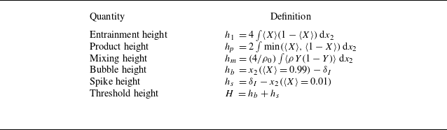
Definitions of mixing layer heights. Here
 $X$
and
 $Y$
are the mole and mass fractions of the heavy fluid;
 $\rho _0= 2\rho _H \rho _L/(\rho _H+\rho _L)$
is a normalization density;
 $\delta _I$
is the initial interface location. All integrals are taken from
 $x_2=-\infty$
to
 $x_2=+\infty$
and
 $\langle \boldsymbol{\cdot }\rangle$
represents an ensemble average.

Following the onset of linear instability, nonlinear effects become dominant, and a turbulent mixing layer develops. In an infinitely large domain, the flow eventually reaches a late-time state of self-similar growth, where viscosity and diffusivity no longer influence the large-scale evolution, and the flow dynamics become independent of its initial conditions (Youngs Reference Youngs1984; Cook, Cabot & Miller Reference Cook, Cabot and Miller2004). Youngs (Reference Youngs1984) initially proposed an expression for the growth of the mixing layer height
 $h_i(t)$
as
 \begin{align} h_i = F_i(A)gt^2, \end{align}
where
 $F_i(A)$
is an unspecified function of the Atwood number (or density ratio). Any large-scale height definition should satisfy (1.3), but the expression for
 $F_i$
depends on this choice. Several common height definitions are listed in table 1. By assuming that the time scales of the turbulent mixing layer growth are proportional to the time scales of the inviscid modal growth associated with (1.1), Youngs obtained the now well-known expression
 \begin{align} h_i \approx \alpha _i A g t^2, \end{align}
where
 $\alpha _i$
is a dimensionless growth parameter whose numerical value depends on the height definition, and
 $t$
is measured relative to a virtual time origin that depends on the initial conditions (Snider & Andrews Reference Snider and Andrews1994; Thévenin et al. Reference Thévenin, Gréa, Kluth and Nadiga2025). Independently, by applying a self-similar ansatz to the governing equations in the Boussinesq limit (i.e.
 $A \ll 1$
or
 $R\approx 1$
), Ristorcelli & Clark (Reference Ristorcelli and Clark2004) derived an expression for the growth rate as
 $\dot {h}_i^2 \propto A g h_i$
, where
 $\dot {h}_i = \textrm {d}h_i/\textrm {d}t$
. By selecting the constant of proportionality as
 $4\alpha _i$
, this relation becomes consistent with (1.4) and can be written as
 \begin{align} \dot {h}_i^2 = 4 \alpha _i\kern-1pt A g h_i. \end{align}
A different functional dependence of the mixing layer height on the density ratio was proposed much earlier by Belen’kii & Fradkin (Reference Belen’kii and Fradkin1965). Their theoretical analysis was built on three key assumptions. First, turbulent kinetic energy (TKE),
 $k$
, scales with potential energy. Second, the flow can be described using a turbulent diffusivity of the form
 $D_t \propto \sqrt {k_t}h_i$
. Third, for sufficiently small density ratios (
 $R\lesssim 4$
), a self-similar solution for the mean density yields an analytical expression for the mixing layer height:
 $h_i \propto (\ln R) g t^2$
, or equivalently,
 \begin{align} \dot {h}_i^2 \propto (\ln R) gh_i. \end{align}
1.1. Atwood number effects
Although Belen’kii & Fradkin (Reference Belen’kii and Fradkin1965) is commonly credited as an early proponent of
 $h\propto gt^2$
scaling, the associated
 $\ln R$
dependence has, to our knowledge, not been adopted in modern RT studies. This may be due to the original work being published in Russian and thus less accessible to the broader research community, or due to the rather specific assumptions involved that are difficult to verify without detailed data from high-Atwood-number RT flows. Instead, variable-density RT studies have been consistently presented in terms of
 $\alpha$
values based on (1.4) and (1.5), even though neither the small-density-variation nor the small-amplitude assumptions hold.
As a result, it has been consistently observed in both experiments (Dimonte & Schneider Reference Dimonte and Schneider2000; Banerjee, Kraft & Andrews Reference Banerjee, Kraft and Andrews2010) and simulations (Youngs Reference Youngs2013; Zhou & Cabot Reference Zhou and Cabot2019) that
 $\alpha _i$
increases with Atwood number, provided
 $\alpha _i$
is defined using the full extent of the mixing layer. Specifically, bubble growth, represented by
 $\alpha _b$
, is largely unaffected by the Atwood number, but spike growth
 $\alpha _s$
increases with the Atwood number. Overall, the growth parameter of the full mixing layer increases with Atwood number, while exhibiting Atwood-number-dependent asymmetries that can be described by
 $\alpha _s/\alpha _b$
. Such asymmetries are not limited to the growth parameter and are also observed in one-dimensional (1-D) planar-averaged density statistics. For instance, 1-D profiles of mixing parameters become more asymmetric as the Atwood number increases, although the nature of such asymmetries depends on the specific definition of mixedness considered (Livescu Reference Livescu2013; Youngs Reference Youngs2013). In terms of volume-averaged mixedness, Zhou, Cabot & Thornber (Reference Zhou, Cabot and Thornber2016) found that those defined in terms of the mole fraction exhibit little sensitivity to the Atwood number, while mass-fraction-based measures decrease systematically as
 $A$
increases.
In the RT literature, statistics associated with the velocity field are less commonly reported. When they are, they often lack consistent normalization with respect to global flow parameters, which hinders meaningful comparisons between different studies. As an illustration, velocity fluctuations have been normalized using
 $\dot {h}$
(Zhou & Cabot Reference Zhou and Cabot2019),
 $(A g h)^{1/2}$
(Akula & Ranjan Reference Akula and Ranjan2016),
 $Agt$
(Banerjee et al. Reference Banerjee, Kraft and Andrews2010) as well as scales based on the initial conditions of the simulation (Livescu et al. Reference Livescu, Ristorcelli, Petersen and Gore2010). Perhaps due to the aforementioned issues, there have been surprisingly few comparative studies of velocity profiles across different Atwood numbers. Based on the findings of Livescu et al. (Reference Livescu, Ristorcelli, Petersen and Gore2010), the primary effect of an increase in the Atwood number is a shift in the peaks of the Favre-averaged velocity and TKE towards the light-fluid side of the mixing layer.
1.2. Reynolds number effects
The late-time self-similar expressions in (1.4) and (1.5) also suggest that the growth parameter is independent of time (and equivalently, the Reynolds number). In a finite domain, this self-similar state is only observed over a limited time window when the mixing layer height is sufficiently larger than the wavelengths of the initial perturbations (Ramaprabhu, Dimonte & Andrews Reference Ramaprabhu, Dimonte and Andrews2005; Banerjee & Andrews Reference Banerjee and Andrews2009; Mueschke & Schilling Reference Mueschke and Schilling2009; Youngs Reference Youngs2013), while remaining small enough such that domain confinement effects are not significant (Dalziel et al. Reference Dalziel, Patterson, Caulfield and Coomaraswamy2008; Boffetta, De Lillo & Musacchio Reference Boffetta, De Lillo and Musacchio2012). Given the appropriate initial conditions, regions of near-constant
 $\alpha _i$
values have been observed for many temporally growing RT simulations at sufficiently late times. However, in several studies (Cabot & Cook Reference Cabot and Cook2006; Burton Reference Burton2011; Zhou & Cabot Reference Zhou and Cabot2019), there appears to be a slight increase in
 $\alpha _i$
values towards the end of the simulation. Similar effects are observed for mixing parameters (Zhou et al. Reference Zhou, Cabot and Thornber2016), where a near-constant region is clearly observed but small fluctuations persist. It remains unclear whether these variations arise due to the growing Reynolds number, the diminishing influence of the initial conditions or the effects of domain boundaries. Another global parameter that is often studied is the ratio of total kinetic energy to total potential energy loss. This ratio has been observed to exhibit a weak dependence on the Reynolds number (Cabot & Cook Reference Cabot and Cook2006; Goh & Blanquart Reference Goh and Blanquart2025), which is commonly described as a non-equilibrium effect stemming from the increasing time lag between production and dissipation at higher Reynolds numbers.
1.3. Statistically stationary RT flow configuration
A key impediment to resolving the open questions discussed above is the lack of high-quality self-similar RT flow data. Although the conditions for achieving late-time self-similar growth are now well understood, the transient behaviour remains poorly characterized. Different flow quantities reach self-similarity at different times, and this issue is exacerbated at higher Atwood numbers, where convergence to self-similarity tends to be delayed (Burton Reference Burton2011). It remains uncertain whether any temporally growing RT (TRT) simulation has fully attained a self-similar state that is truly independent of the initial conditions and domain boundaries, particularly at high Atwood numbers. This issue is discussed in detail by Schilling (Reference Schilling2020). For a temporally growing mixing layer, the only path towards addressing these questions about the self-similar state seems to involve longer simulation times, larger domains and ballooning computational costs.
Many of these challenges are substantially mitigated by the statistically stationary RT (SRT) flow configuration proposed by Goh & Blanquart (Reference Goh and Blanquart2025). A more detailed summary is provided in § 2, but a brief introduction is presented here to highlight its computational advantages. In essence, the SRT configuration approximates the unsteady dynamics of a temporally growing RT mixing layer in a transformed coordinate system where the transformed dynamics are statistically stationary. The resulting flow can be evolved over arbitrarily long simulation times on a fixed grid, generating a continuous stream of flow realizations and yielding converged statistics that are independent of initial conditions. Under specific domain dimensions, the SRT configuration functions as a minimal flow unit (MFU) for self-similar TRT flows, where the statistics of self-similar TRT flows are reproduced to a reasonable accuracy, while resolving only the high wavenumber components of turbulence. Besides eliminating the cost associated with a growing Reynolds number, the SRT MFU requires only a fraction of the grid points for a typical self-similar TRT simulation at the same Reynolds number, making it an efficient surrogate for exploring higher Atwood number regimes at considerably lower computational cost.
1.4. Objectives
The primary objective of this study is to investigate the influence of Atwood and Reynolds numbers on SRT flow, and verify their applicability to self-similar TRT flows where possible. The analysis focuses on planar-averaged profiles of the dominant non-transport terms in the continuity, mixed mass and TKE budgets. We seek to distinguish between global (or integral) and local (or shape) effects: global effects are reflected in the integral properties of the profiles and can be accounted for by appropriate normalization, while local effects may persist after normalization and are expressed through the shape of the normalized profiles. Normalizations will be developed through a combination of theoretical arguments and empirical observations, with the goal of identifying near-universal non-dimensional quantities that hold across a broad parameter space. Through this analysis, we aim to provide further context to some of the questions posed earlier in this section and suggest alternatives to conventional approaches.
The paper is organized as follows. In § 2, the SRT configuration is introduced through a review of Goh & Blanquart (Reference Goh and Blanquart2025), and the methodology is extended to different Atwood numbers. Section 3 details the simulation cases and numerical methods, and compares SRT results with TRT results. In § 4, normalizations for all dominant budget terms are proposed, and the normalized profiles analysed. Section 5 builds on these results to explore three related topics: (i) the derivation of a reference density for the mixed mass; (ii) the effects of the Atwood number on Favre-averaged velocity statistics; (iii) a proposed scaling law for the mixing layer growth rate that generalizes (1.5) to variable-density flows. Finally, § 6 summarizes the key findings and discusses their broader implications.
2. Mathematical description
The SRT flow configuration is first introduced through a review of the governing equations in § 2.1, followed by a summary of its flow properties in § 2.2. Complete details on the mathematical derivation, assumptions and validation of the computational framework can be found in Goh & Blanquart (Reference Goh and Blanquart2025). In § 2.3, the input parameters for the present study are discussed.
2.1. Governing equations
The governing equations for SRT flow are derived through two main steps. First, by leveraging the anticipated self-similar behaviour of turbulent RT mixing layers at late times, a transformation of the vertical coordinate and velocities is applied to the low-Mach-number Navier–Stokes equations (NSE). Second, these transformed equations are then evaluated at a specified time
 $t=t_0$
, leading to simplified equations in the transformed coordinates that resemble the original NSE, but include two sets of additional terms. The SRT governing equations corresponding to continuity, scalar and momentum transport are
 \begin{align} \frac {\partial \rho }{\partial s} + \frac {\partial \rho u_{\kern-1.5pt j}}{\partial x_{\kern-1.5pt j}} &= \frac {y}{\tau _0}\frac {\partial \rho }{\partial y}, \\[-28pt] \nonumber \end{align}
 \begin{align} \frac {\partial \rho Y}{\partial s} + \frac {\partial \rho u_{\kern-1.5pt j}\kern-0.5pt Y}{\partial x_{\kern-1.5pt j}} &= \frac {\partial }{\partial x_{\kern-1.5pt j}}\left (\rho D \frac {\partial Y}{\partial x_{\kern-1.5pt j}}\right ) +\frac {y}{\tau _0}\frac {\partial \rho Y}{\partial y}, \\[-28pt] \nonumber \end{align}
 \begin{align} \frac {\partial \rho u_i}{\partial s} + \frac {\partial \rho u_{\kern-1.5pt j} u_i}{\partial x_{\kern-1.5pt j}} = -\frac {\partial p}{\partial x_i} + \frac {\partial \tau _{\textit{ij}}}{\partial x_{\kern-1.5pt j}} - \rho g \delta _{2i} + \frac {y}{\tau _0}\frac {\partial \rho u_i}{\partial y} - \frac {1}{2\tau _0}\rho u_i, \\[-12pt] \nonumber \end{align}
where
 $Y$
is the mass fraction of the heavy fluid,
 $D$
is the kinematic diffusivity,
 $u_i$
are the velocity components and
 $p$
is the hydrodynamic pressure. In the SRT framework,
 $s$
is the simulation time in the transformed coordinate system, and
 $\tau _0$
is an SRT-specific flow parameter. The shear stress tensor
 $\tau _{\textit{ij}}$
is defined as
 \begin{align} \tau _{\textit{ij}} = \rho \nu \left [\frac {\partial u_i}{\partial x_{\kern-1.5pt j}} + \frac {\partial u_{\kern-1.5pt j}}{\partial x_i} - \frac {2}{3} \frac {\partial u_{\kern-1.5pt j}}{\partial x_k}\delta _{\textit{ij}}\right ]\!, \end{align}
where
 $\nu$
is the kinematic viscosity and
 $\delta _{\textit{ij}}$
is the Kronecker delta. Relating mass fraction to density, the low-Mach-number equation of state is
 \begin{align} \rho (Y) = \frac {\rho _H \rho _L}{\rho _H- (\rho _H-\rho _L)Y}, \quad \textrm {or} \quad Y(\rho ) = \frac {\rho _H (\rho - \rho _L)}{\rho (\rho _H - \rho _L)}. \end{align}
Two sets of source terms appear on the right-hand side of (2.1)–(2.3). The first set of source terms, denoted generally as
 $S_\phi$
, is derived from rescaling the vertical coordinate, and appears in all three transport equations, (2.1)–(2.3), in the form
 \begin{align} S_\phi = \frac {y}{\tau _0}\frac {\partial \rho \phi }{\partial y}, \end{align}
where
 $\phi = 1, u_i, \textrm {or } Y$
. In (2.6),
 $y=x_2-\hat {\delta }_I$
is the vertical coordinate relative to the location of the initial interface, which is specified by the input
 $\hat {\delta }_I$
. Practically, the input
 $\hat {\delta }_I$
can be used to shift the mixing layer relative to the computational domain. Beyond this use (which is briefly discussed in § 3.1),
 $y$
and
 $x_2$
can be treated equivalently. The second set of source terms arises from velocity scaling and appears only in the momentum equations, (2.3), as
 \begin{align} T_i = -\frac {1}{2\tau _0} \rho u_i. \end{align}
The eventual height of the statistically stationary mixing layer is determined by the time scale parameter
 $\tau _0$
, which is found in both sets of source terms defined in (2.6) and (2.7). In Goh & Blanquart (Reference Goh and Blanquart2025),
 $\tau _0$
was implemented using an input mixing height
 $\hat {h}_m$
and the closure equation
 \begin{align} \frac {1}{\tau _0 (s)} = \frac {4}{\rho _0 \hat {h}_m} \int \langle \rho \chi \rangle _{1,3}\,\textrm {d}y, \end{align}
where
 $\langle \boldsymbol{\cdot }\rangle _{1,3}$
denotes an instantaneous planar average over the
 $x_1$
and
 $x_3$
directions,
 $\chi =2D(\partial Y/\partial x_i)^2$
is the local scalar dissipation rate and
 $\rho _0 = 2\rho _H \rho _L/(\rho _H+\rho _L)$
is the harmonic mean of the reservoir densities, arbitrarily chosen as a normalization density. All integrals in this paper are evaluated over the entire domain. By solving (2.1)–(2.5) and (2.8), a statistically stationary flow is achieved.
2.2. Properties of SRT flow
To provide further context, the following section summarizes several key aspects of the SRT configuration and discusses its relationship with the TRT flow configuration.
-
(i) As mentioned earlier, the derivation of the governing SRT equations involves two main steps. The first step represents a simple shrinking of the flow in the vertical direction. The transformed equations remain valid for all
 $t$
and can be solved in the transformed variables to achieve a fixed height. However, the small scales would continue to shrink, and direct numerical simulations (DNS) of such a ‘rescaled TRT’ configuration would still need to resolve the growing range of scales, offering no computational benefit to a traditional TRT simulation. The second step involves evaluating the ‘rescaled TRT’ equations at a fixed time
$t=t_0$
, which yields the final form of the SRT equations, (2.1)–(2.3). This approximation is crucial, as it enables stationarity not just in the large scales but also at the small scales.
-
(ii) The additional terms
$S_\phi$
and
$T_i$
oppose the underlying TRT growth that is driven by the NSE terms. The term
$S_\phi$
is zero in the core of the mixing layer (
$y=0$
), most active near the edges of the mixing layer, and zero in the fluid reservoirs (no gradients);
$T_i$
has no explicit dependence on the spatial coordinates. On average, the source terms remove kinetic energy from the flow at a rate proportional to
$1/\tau _0$
. In spectral space (defined only in the homogeneous directions), this removal of energy is directly proportional to the in-plane kinetic energy spectra and preserves the wavenumber distribution of kinetic energy at each vertical location (see Appendix A). -
(iii) Although the height of the SRT mixing layer does not grow as the simulation progresses, the time average of the SRT parameter
$\bar {\tau }_0$
(an overline denotes a time average) corresponds to the growth time scale of the mixing layer height in an equivalent TRT flow. Hence, any mention of growth rates or parameters for the SRT configuration is not literal, but should be interpreted in the context of its equivalent TRT configuration. In a self-similar TRT flow, all height definitions
$h_i$
would grow proportionally to each other and have the same time scale. This is expressed mathematically as(2.9)By combining (1.5) and (2.9),
\begin{align} \left [ \frac {1}{\bar {\tau }_0} \right ]_{\textit{SRT}} = \left [\frac {\dot {h}_i(t_0)}{h_i(t_0)} \right ]_{\textit{TRT}} \!. \end{align}
$\bar {\tau }_0$
is related to the height of the equivalent TRT flow by(2.10)
\begin{align} h_i(t_0) = 4\alpha _i\kern-0.5pt Ag\bar {\tau }_0^2. \end{align}
-
(iv) When solving the SRT equations,
$\tau _0$
can either be prescribed as a constant input or implemented through a closure equation and a secondary input. If prescribed as a constant
$\hat {\tau }_0$
, the mixing layer grows until
$h(s)$
reaches a statistically stationary value that is not known a priori. Alternatively, using the closure (2.8) with an input height
$\hat {h}_m$
ensures that the instantaneous mixing layer height(2.11)convergences to the constant input
\begin{align} h_m(s) = \frac {4}{\rho _0}\int \langle \rho Y (1-Y) \rangle _{1,3} \,{\textrm {d}}y \end{align}
$\hat {h}_m$
. As shown by Goh & Blanquart (Reference Goh and Blanquart2025), the choice of method does not impact the converged flow statistics. That being said, an input height is preferable to an input time scale. First, the mixing layer height is an intuitive and common reference in the RT literature. Second, a given height allows the user to define the computational grid efficiently without needing to iterate or allocate excess grid cells.
-
(v) Similar to observations from other statistically stationary configurations (Rosales & Meneveau Reference Rosales and Meneveau2005; Chung & Pullin Reference Chung and Pullin2010; Carroll & Blanquart Reference Carroll and Blanquart2015; Dhandapani & Blanquart Reference Dhandapani and Blanquart2020), the SRT configuration exhibits box-filling tendencies in the homogeneous directions. In a domain of lateral size
$\mathcal{L}_{\textit{SRT}}$
, the largest flow structures are expected to expand laterally over time and eventually interact with the periodic boundaries, leading to the formation of a single large-scale structure or MFU. In this statistically stationary state, the integral length scales of the flow are bounded vertically by
$\ell _2 \sim \hat {h}$
and horizontally by
$\ell _1 \sim \mathcal{L}_{\textit{SRT}}$
, The resulting stationarity of
$\ell _2/\ell _1$
in SRT mirrors that observed in unconfined, self-similar TRT flows, where
$\ell _2/\ell _1$
is approximately constant across Atwood number and Reynolds numbers, despite
$h(t)/\mathcal{L}_{\textit{TRT}}$
growing in time (Zhou & Cabot Reference Zhou and Cabot2019). Because of the dynamical significance of the lateral domain size in SRT flow, the mixing layer aspect ratio
$\hat {h}_m/\mathcal{L}_{\textit{SRT}}$
affects not only the integral length scales, but also other global quantities, e.g.
$\alpha$
and mixedness. For
$A=0.5$
, all SRT flow statistics obtained at
$\bar {h}_m/\mathcal{L} \approx 1.5$
show good agreement with self-similar TRT flow. -
(vi) In an unconfined TRT flow, a large domain allows the growing mixing layer sufficient time to approach its intrinsic large-scale aspect ratio through mode-coupling processes. In a confined SRT configuration,
$\mathcal{L}_{\textit{SRT}}$
(along with input height
$\hat {h}$
) constrains the flow and selects
$\ell _2/\ell _1$
directly. Consequently, the SRT configuration does not resolve the very large scales (or infrared range) of a TRT flow and the backscatter-dominated dynamics of that wavenumber range (Soulard, Griffond & Gréa Reference Soulard, Griffond and Gréa2015). Hence, the SRT MFU identified in (v) is only an approximate representation of self-similar TRT flow in the range of wavenumbers beyond the peak of the TRT energy spectrum, as evident from figure 19 of Goh & Blanquart (Reference Goh and Blanquart2025). Like other MFU configurations (Jiménez & Moin Reference Jiménez and Moin1991; Hamilton, Kim & Waleffe Reference Hamilton, Kim and Waleffe1995; Flores & Jiménez Reference Flores and Jiménez2010; Hsieh & Biringen Reference Hsieh and Biringen2016), the large scales are ‘filtered’ out by computational confinement, and the remaining scales capture sufficient dynamics to reproduce the turbulence statistics of interest. -
(vii) Since all statistics in the SRT coordinate system are stationary, the SRT configuration can be simulated indefinitely. The flow has a finite time memory, which can be quantified by its integral time scale
$\tau _{{int}}$
. After
$\Delta s \sim \tau _{{int}}$
, the flow becomes decorrelated, and a subsequent, independent realization of the flow begins, each of which are representative of TRT flow in the vicinity of
$t=t_0$
. Over simulation time
$s$
, SRT flow generates continuous, independent realizations of a single large-scale structure which are equivalent to realizations (generated over
$x_1$
,
$x_3$
and initial conditions) in a TRT flow ensemble at a specific time. Mathematically, any flow quantity
$\varOmega$
averaged over
$x_1$
,
$x_3$
and
$s$
in SRT flow is (approximately) equal to its ensemble average in TRT flow at time
$t_0$
,(2.12)Henceforth, unless the domain of averaging is specified as a subscript,
\begin{align} \langle \varOmega _{\textit{SRT}} \rangle _{1,3,s}(y) \approx \langle \varOmega _{\textit{TRT}} \rangle (t_0,y). \end{align}
$\langle \boldsymbol{\cdot }\rangle = \langle \boldsymbol{\cdot }\rangle _{1,3,s}$
is assumed for SRT flow. Finally, due to its finite time memory, converged SRT flow is independent of its initial conditions. In practice, this is typically achieved within
$s\lt 5\tau _0$
.


2.3. Input parameters
To extend the framework from Goh & Blanquart (Reference Goh and Blanquart2025) to a range of Atwood numbers, a different input height definition from (2.11) is chosen. The reasons for this choice are first presented, followed by a summary of all non-dimensional inputs.
2.3.1. Input height
The mixing height
 $h_m$
, defined in (2.11), includes the density within the integral and thus requires a reference density for normalization; this reference density generally depends on the reservoir densities
 $\rho _H$
and
 $\rho _L$
. In Goh & Blanquart (Reference Goh and Blanquart2025), this reference density was chosen arbitrarily as the harmonic mean of the reservoir densities
 $\rho _0$
. Because all simulations were conducted at the same reservoir densities (i.e. same Atwood number), the choice of normalization density did not influence the results. In contrast, in the present study, the Atwood number (and consequently, at least one of
 $\rho _H$
and
 $\rho _L$
) is varied; the physically appropriate normalization density is not an obvious one. To ensure consistency across SRT configurations of different Atwood numbers, a different height definition that does not require an arbitrary density normalization is used.
Heights can be defined in terms of the mole fraction,
 $X = (\rho -\rho _L)/\Delta \rho$
, or the mass fraction
 $Y$
. In the analytical self-similar solution for 1-D variable-density diffusion (shown in Appendix B), the mole fraction profile
 $X(y/h_1)$
does not change with Atwood number, but the mass fraction profile does. For three-dimensional (3-D), turbulent SRT flow, it will be shown in § 4.1.1 that this observation remains true. More specifically, the mean mole fraction
 $\langle X \rangle$
is approximately constant with respect to the Atwood number, but the Favre average of the mass fraction is not. Therefore, we seek height definitions that involve only the mean mole fraction.
There are several common height definitions based on the mean mole fraction. These include the entrainment height,
 $h_1 = 4\int \langle X \rangle (1-\langle X \rangle ) \,{\textrm {d}}y$
, the product height,
 $h_{\kern-1pt p} = 2\int \min (\langle X \rangle ,\langle 1-X \rangle ) \,{\textrm {d}}y$
, or threshold-based heights that are derived from the
 $y$
-locations of the mean mole fraction field at specified thresholds, e.g.
 $H = y(\langle X\rangle =0.99) - y(\langle X\rangle =0.01)$
. Threshold-based heights are determined from averages on a single plane and are more prone to statistical noise. Conversely, integral height definitions are computed over the entire domain. Between the two integral heights mentioned, we choose to use
 $h_1$
because its integrand varies smoothly with
 $\langle X \rangle$
and an analytical equation for its time evolution can be derived. This leads to a closure equation for
 $\tau _0$
that functions similarly to (2.8), but for a prescribed input
 $\hat {h}_1$
instead of
 $\hat {h}_m$
,
 \begin{align} \frac {1}{\tau _0(s)} = \frac {8}{\Delta \rho \hat {h}_1} \int \langle X \rangle _{1,3} \frac {\partial \langle \rho v \rangle _{1,3}}{\partial y} {\textrm {d}}y. \end{align}
The derivation of this closure equation is presented in Appendix C. Solving (2.13) alongside (2.1)–(2.5),
 $h_1(s)$
converges to a constant value, and
 $\bar {h}_1 \approx \hat {h}_1$
.
The MFU aspect ratio of
 $\bar {h}_m/\mathcal{L}=1.5$
for
 $A = 0.5$
quoted by Goh & Blanquart (Reference Goh and Blanquart2025) corresponds to
 $\bar {h}_1/\mathcal{L} = 1.7$
. In the present study, we seek to keep
 $\bar {h}_1/\mathcal{L}=1.7$
approximately constant while studying the effect of other parameters.
2.3.2. Non-dimensional inputs
The SRT equations, (2.1)–(2.3), require the specification of gravity (
 $g$
) and fluid properties (
 $\rho _H$
,
 $\rho _L$
,
 $\nu$
,
 $D$
), while the closure equation, (2.13), requires input
 $\hat {h}_1$
. Additionally, as discussed in § 2.2, the lateral domain size
 $\mathcal{L}$
is physically significant in SRT flow, while the initial conditions are not. In accordance with the Buckingham Pi theorem, the flow can be fully defined by four non-dimensional numbers,
 \begin{align} A = \frac {\rho _H-\rho _L}{\rho _H+\rho _L}, \quad Sc = \frac {\nu }{D}, \quad Gr = \frac {A g\hat {h}_1^3}{\nu ^2}, \quad \lambda = \frac {\hat {h}_1}{\mathcal{L}}, \end{align}
where
 $A$
is the Atwood number,
 $Sc$
the Schmidt number,
 $ \textit{Gr}$
the Grashof number and
 $\lambda$
the aspect ratio of the mixing layer. In the present study, the Atwood and Grashof numbers are varied, while
 $Sc$
and
 $\lambda$
are held constant.
The choice of these non-dimensional quantities is not unique. First, the density ratio
 $R$
could have been used instead of
 $A$
. They are uniquely related by (1.2) and either choice is equivalent. Second, the inclusion of
 $A$
in the definition of the Grashof number is based on convention. While
 $ \textit{Gr}$
is listed as the input parameter in (2.14), the results are primarily presented in terms of the output Reynolds number. Both the Grashof number and the Reynolds number characterize the ratio of the buoyancy-driven large scales to the viscous scales and their values correlate with turbulence intensity. However, the Reynolds number is preferred because it is more commonly used in the turbulence literature and widely understood beyond the field of buoyancy-driven flows. It is defined in terms of the time-averaged output parameters as
 \begin{align} Re = \frac {\bar {h}_1^2}{\bar {\tau }_0\nu }. \end{align}
To maintain consistency throughout this paper,
 $h_1$
is used in (2.15), but any large-scale height definition would be reasonable for a self-similar RT flow. For instance, a Reynolds number based on
 $H$
was used in Cabot & Cook (Reference Cabot and Cook2006) and Goh & Blanquart (Reference Goh and Blanquart2025).
3. Simulation cases and numerical method
This section is divided into three parts. First, the set-up of the computational domain and the list of simulation cases are presented. Second, the numerical method is described. Finally, several global parameters are compared between SRT and self-similar TRT results, extending the comparisons beyond what was done by Goh & Blanquart (Reference Goh and Blanquart2025) for
 $A=0.5$
.
3.1. Simulation cases
Simulations are performed on a 3-D rectangular domain. The top and bottom boundaries are implemented as Dirichlet boundary conditions and the lateral boundaries as periodic. The computational grid is centred at
 $x_i=0$
with domain lengths
 $\mathcal{L}_i$
and grid spacing
 $\Delta _i$
. In the horizontal directions,
 $\mathcal{L}_1= \mathcal{L}_3=\mathcal{L}$
, and
 $\Delta _1 = \Delta _3 = \mathcal{L}/N_1$
, where
 $N_1=N_3$
is the number of grid points in each direction. In all simulations,
 $\mathcal{L} = 1$
is fixed. In the vertical direction,
 $\Delta _2$
varies with
 $x_2$
. A uniformly spaced (
 $\Delta _2 = \Delta _1$
) core grid of length
 $\mathcal{L}_{2c} = N_{2c}\Delta _1$
is used to resolve the bulk of the mixing layer (
 $|x_2|\leqslant \mathcal{L}_{2c}/2$
). This core grid region is defined to be at least 10 % wider than the region that contains the 1 % and 99 % mean mole fraction locations. Because of known asymmetries associated with high Atwood number flows (Cabot & Zhou Reference Cabot and Zhou2013; Zhou & Cabot Reference Zhou and Cabot2019), the optional parameter
 $\hat {\delta }_I$
is used to shift the mixing layer so that it lies within the refined core grid. Outside the core, the vertical spacing
 $\Delta _2(x_2)$
is stretched with a factor of 1.1, and the total domain height satisfies the condition
 $\mathcal{L}_2\gt 4\mathcal{L}_{2c}$
. In the vertical direction, the results were verified to be insensitive to a larger domain or core grid region.
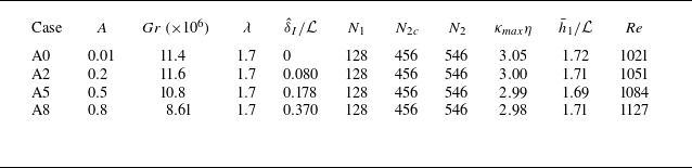
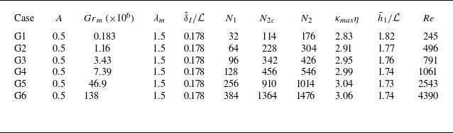
A list of the simulation cases considered in this study is summarized in tables 2 and 3. All simulations are performed at
 $Sc = 1$
with constant
 $\nu$
and
 $D$
. Table 2 summarizes the set of new simulations in which the Atwood number is varied at approximately constant
 $Re \approx 1100$
, while table 3 lists the simulation cases from Goh & Blanquart (Reference Goh and Blanquart2025) where Reynolds number was varied at constant
 $A = 0.5$
. As discussed in § 2.1, the input height used by Goh & Blanquart (Reference Goh and Blanquart2025) was
 $\hat {h}_m$
, and the associated non-dimensional inputs were
 $A$
,
 $Sc$
,
 $Gr_m = Ag\hat {h}_m^3/\nu ^2$
and
 $\lambda _m = \hat {h}_m/\mathcal{L}$
. To account for this difference in definitions, each set of simulations is listed in terms of their respective input parameters, but output values of
 $\bar {h}_1/\mathcal{L}$
and
 $ \textit{Re} $
are included in the final two columns for a consistent comparison.
Simulation cases performed in the current study using
 $\hat {h}_1$
as the input.

Simulation cases from Goh & Blanquart (Reference Goh and Blanquart2025) performed using
 $\hat {h}_m$
as the input.

In table 2, A0–A8 have increasing Atwood numbers with A0 representing the Boussinesq limit. The Grashof number is reduced with increasing Atwood number to ensure that the ratio
 $\bar {h}_1/\eta$
is constant, where
 $\eta = (\nu ^3/\tilde {\epsilon })^{1/4}$
is the Kolmogorov scale and
 $\tilde {\epsilon }$
is the Favre-averaged viscous dissipation (defined later in (4.8)). Doing so results in a near-constant Reynolds number across Atwood numbers. Although the variation in the Grashof number is not large,
 $ \textit{Gr}$
does not scale directly with
 $\bar {h}_1/\eta$
or
 $ \textit{Re} $
due to the somewhat arbitrary inclusion of
 $A$
in its definition. This slight difference in trends between
 $ \textit{Re} $
and
 $ \textit{Gr}$
is explained in § 5.3.
In table 3, the Reynolds number increases from G1 to G6. There is a gradual decrease of the aspect ratio
 $\bar {h}_1/\mathcal{L}$
with Reynolds number; this is because
 $\hat {h}_m$
was used as the input parameter and
 $h_1$
was not prescribed directly. It will be shown in § 4.1 that the small differences in
 $\bar {h}_1/\mathcal{L}$
do not affect the results, once quantities are suitably normalized.
To ensure that simulations are well-resolved, all simulations are performed at
 $\kappa _{\textit{max}}\eta \gtrsim 3.0$
, where
 $\kappa _{\textit{max}} = \pi /\Delta _2$
is the maximum resolved wavenumber. The minimum values of
 $\kappa _{\textit{max}}\eta$
across the mixing layer are listed in tables 2 and 3.
3.2. Numerical method
Simulations are performed using the computational solver, NGA (Desjardins et al. Reference Desjardins, Blanquart, Balarac and Pitsch2008). The numerical code solves the conservative-variable formulation of the low-Mach-number NSE with staggered finite difference operators and uses a fractional step method to enforce continuity. The NSE are solved using a second-order semi-implicit iterative midpoint scheme and uses staggering in time between the momentum field and the scalar and density fields. The scalar is advanced first, the density field is updated, and the momentum equations are then advanced. The resulting computational framework conserves kinetic energy discretely (i.e. there is no numerical viscosity).
The bounded cubic Hermite polynomial (BCH) scheme (Verma, Xuan & Blanquart Reference Verma, Xuan and Blanquart2014) is used for scalar transport. This scheme was chosen because it ensures scalar boundedness and has less numerical diffusion than other schemes, including weighted essentially non-oscillatory schemes. In particular, Verma et al. (Reference Verma, Xuan and Blanquart2014) found that other bounded schemes require at least twice the spatial resolution to resolve small-scale scalar features as well as the BCH scheme. The Courant–Friedrichs–Lewy condition of
 ${\textrm {CFL}}\leqslant 0.8$
is imposed for all simulations in the current study. Further details on the implementation of the original NSE and scalar transport can be found in Desjardins et al. (Reference Desjardins, Blanquart, Balarac and Pitsch2008) and Verma et al. (Reference Verma, Xuan and Blanquart2014), while the implementation of the SRT terms
 $S_\phi$
and
 $T_i$
is addressed by Goh & Blanquart (Reference Goh and Blanquart2025).
3.3. Comparison with self-similar TRT
The SRT results for
 $A=0.5$
,
 $\lambda =1.7$
have been validated comprehensively against TRT studies by Goh & Blanquart (Reference Goh and Blanquart2025). We extend the analysis here to other Atwood numbers. In particular, it is crucial to verify that
 $\lambda =1.7$
remains the MFU for self-similar RT turbulence for the range of Atwood numbers considered. To this end, global parameters obtained from the SRT results for
 $A=$
0.2, 0.5 and 0.8 are compared with similar quantities from DNS studies of self-similar TRT flows (Zhou et al. Reference Zhou, Cabot and Thornber2016; Zhou & Cabot Reference Zhou and Cabot2019). The TRT-equivalent growth parameter
 $\alpha _p$
is computed using (2.10) and the definition of
 $h_{\kern-1pt p}$
(see table 1), while the mixing parameters are defined as
 \begin{align} \varXi = \frac {\int \langle \min (X,1-X)\rangle \,{\textrm {d}}y}{\int \min (\langle X \rangle , \langle 1- X \rangle ) \,{\textrm {d}}y}, \\[-28pt] \nonumber \end{align}
 \begin{align} \varTheta = \frac {\int \langle X(1-X) \rangle \,{\textrm {d}}y}{\int \langle X \rangle (1- \langle X \rangle ) \,{\textrm {d}}y}, \\[-28pt] \nonumber \end{align}
 \begin{align} \varPsi = \frac {\int \langle \rho Y (1-Y) \rangle \,{\textrm {d}}y}{\int \langle \rho \rangle \langle Y \rangle (1-\langle Y \rangle ) \,{\textrm {d}}y}. \\[-2pt] \nonumber \end{align}
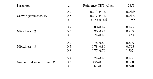
The reference TRT values in table 4 are obtained from figure 2 of Zhou et al. (Reference Zhou, Cabot and Thornber2016) and figure 5 of Zhou & Cabot (Reference Zhou and Cabot2019).
Comparison of global parameters between SRT and self-similar TRT simulations (Zhou et al. Reference Zhou, Cabot and Thornber2016; Zhou & Cabot Reference Zhou and Cabot2019).

Comparisons involving TRT values should be considered in the context of two main issues. First, there is no established criteria for determining the onset of self-similarity in a TRT flow. The reference TRT values in table 4 correspond to the range of values observed for
 $t\gt 10$
, which is visually estimated to be the time from which global quantities start to vary more slowly in time. Second, there is variability between different studies owing to differences in the initial conditions, lateral confinement effects, numerical methods and data processing. Therefore, comparison of numerical values are typically only meaningful up to one or two significant figures. The observed spread in these global values and the associated issues have been discussed in several review articles (Dimonte et al. Reference Dimonte2004; Zhou Reference Zhou2017; Schilling Reference Schilling2020). The TRT values reported in table 4 are from a single set of simulations and are provided for purposes of comparison rather than validation. Nonetheless, the good agreement between SRT and TRT results indicates that SRT flow at
 $\lambda =1.7$
is an effective MFU for self-similar TRT flow up to
 $\textit {A} = 0.8$
.
4. Results
The ultimate objective of this work is to develop scalings in terms of the dimensional inputs introduced in § 2.3, which are
 $\rho _H$
,
 $\rho _L$
,
 $\nu$
,
 $D$
,
 $g$
and
 $h_1$
. In § 4.1, scalings are initially developed with the introduction of two intermediate global variables: the SRT time scale
 $\tau _0$
and the integrated mixed mass
 $M$
. In § 4.2, expressions for relating each of the intermediate global variables to the input variables are proposed. All scaling relationships are intended to be applicable to both statistically converged SRT flows and late-time TRT flows. To reflect this equivalence, time-averaging in SRT flows is assumed and the overline notation is omitted throughout the remainder of this paper.
4.1. Scaling of SRT budget terms
The ensemble (or Reynolds) average of a general flow variable
 $\phi$
is denoted by
 $\langle \phi \rangle$
and evaluated in SRT flow as averages over the homogeneous directions
 $x_1$
,
 $x_3$
, and time
 $s$
. The density-weighted (or Favre) average of
 $\phi$
is denoted by
 $\tilde {\phi } = \langle \rho \phi \rangle / \langle \rho \rangle$
; the Reynolds and Favre fluctuations are defined as
 $\phi ' = \phi - \langle \phi \rangle$
and
 $\phi '' = \phi - \tilde {\phi }$
, respectively.
Scalings (notated with the
 $\sim$
symbol) are proposed by examining the dominant balances in each of the ensemble-averaged budget equations. Formally, the
 $\sim$
symbol or the phrase ‘scales with’ is interpreted as
 \begin{align} \langle \phi \rangle (y) \sim f \quad \Leftrightarrow \quad \int \langle \phi \rangle \,{\textrm{d}}\left (\frac {y}{h_1}\right )\approx K_{\langle \phi \rangle } \, f, \end{align}
where
 $f = f(h_1, \rho_H, \rho_L, g, \ldots)$
is a dimensional parameter computed from global parameters, and
 $K_{\langle \phi \rangle }$
is a dimensionless constant specific to the field of interest. The spatial coordinate
 $y$
is normalized based on the assumptions of self-similarity (i.e. all length scales vary proportionally to each other) and
 $h_1$
is the only input length scale.
To quantify the collapse of profiles, their spread is quantified using a spatially integrated root-mean-square deviation
 $E_{\textit{rms}}$
. For a quantity
 $\varPhi (y/h_1)$
, this is defined as
 \begin{align} E_{\textit{rms}} = \sqrt {\frac {1}{n}\sum _{i=1}^n \int \left [\varPhi _i(y/h_1) - \bar {\varPhi }(y/h_1) \right ]^2 {\textrm{d}}\left (\frac {y}{h_1}\right )}, \end{align}
where
 $n$
is the number of cases considered and
 $\bar {\varPhi }(y/h_1)$
is the mean profile. A normalized spread
 $\mathcal{E}_{\textit{rms}}$
is defined as one of two possibilities. If
 $\varPhi (\pm \infty )=0$
,
 $E_{\textit{rms}}$
is normalized by the area under the curve of the mean profile,
 $\mathcal{E}_{\textit{rms}} = E_{\textit{rms}}/ |\int \bar {\varPhi } {\textrm{d}}(y/h_1) |$
. If
 $\varPhi \ne 0$
in the fluid reservoirs (e.g. the mole fraction has a value of 1 in the heavy reservoir),
 $E_{\textit{rms}}$
is normalized by the range of
 $\varPhi$
as
 $\mathcal{E}_{\textit{rms}} = E_{\textit{rms}}/(\varPhi _{{max}}-\varPhi _{\textit{min}})$
.
4.1.1. Continuity
First, the scaling of the mean density
 $\langle \rho \rangle$
is considered. In all simulation cases,
 $\rho _H = 1$
is chosen to be constant and
 $\rho _L$
varies according to the Atwood number. As a result, cases A0–A8 have different densities in the light fluid reservoir, evident from the mean density profiles shown in figure 1(a).
A straightforward normalization of the mean density is to stretch its profiles linearly along the vertical axis to take values between 0 and 1; this normalization results precisely in the definition of the heavy fluid mole fraction,
 $\langle X \rangle = (\langle \rho \rangle - \rho _L)/\Delta \rho$
. The mean mole fraction for cases A0–A8 are shown in figure 1(b) and they are approximately independent of Atwood number with
 $\mathcal{E}_{\textit{rms}}\approx 0.02$
. This apparent collapse of the profiles was an important justification for our selection of
 $h_1$
as the length scale for defining the mixing layer aspect ratio (see § 2.3.1). Some Atwood number effects remain noticeable, particularly at the edges of the mixing layer. As the Atwood number increases, gradients are larger on the heavy side of the mixing layer and smaller on the light side. This results in
 $h_s/h_b$
ratios that grow with the Atwood number, which are consistent with observations from other TRT studies (Banerjee et al. Reference Banerjee, Kraft and Andrews2010; Burton Reference Burton2011; Youngs Reference Youngs2013; Akula & Ranjan Reference Akula and Ranjan2016; Zhou & Cabot Reference Zhou and Cabot2019).
Effect of the Atwood number on the (a) mean density, (b) mean mole fraction and (c) Favre-averaged mass fraction. Legend:
 $A=$
0.01 (magenta solid); 0.2 (blue dashed); 0.5 (red dash–dotted); 0.8 (green dotted); analytical 1-D solution (black circles). (d) Effect of the Reynolds number on the mean mole fraction. Legend:
 $Re\approx$
245 (red dotted); 496 (blue dash–dotted); 791 (magenta solid); 1060 (green dashed); 2540 (thick red solid); 4390 (thick black dashed).

Another possible normalization of the mean density is the Favre-average of the mass fraction, which is shown in figure 1(c). The Favre-averaged mass fraction exhibits significant variations with the Atwood number, which is expected because
 $\tilde {Y}$
is algebraically related to
 $\langle X \rangle$
via the equation of state (2.5) such that
 \begin{align} \tilde {Y} = \frac {\rho _H \langle X \rangle }{\langle \rho \rangle } = \frac {R\langle X \rangle }{1 + (R-1)\langle X \rangle }. \end{align}
Based on (4.3), if
 $\langle X \rangle$
is independent of the density ratio
 $R$
, then
 $\tilde {Y}(\langle X \rangle ,R)$
is not. By extension, any function of
 $\tilde {Y}$
is not, in general, independent of
 $R$
. The observed Atwood-invariance of the mean mole fraction (and not the mass fraction) is also consistent with the 1-D variable-density temporal diffusion problem, whose solution is derived in Appendix B and included in figure 1(b).
The effect of the Reynolds number on the mean mole fraction is illustrated in figure 1(d) using cases G1–G6. The profiles appear nearly identical (
 $\mathcal{E}_{\textit{rms}}\approx 0.007$
), indicating that the Reynolds number has a negligible influence on the mean density field.
Based on (4.1), the mean density gradient scales as
 \begin{align} \frac {{\textrm {d}} \langle \rho \rangle }{{\textrm {d}}y} \sim \frac {\Delta \rho }{h_1}. \end{align}
The scaling of the mean mass flux can be determined using the observed scaling of the mean density gradient and the continuity equation, (2.1). The ensemble average of (2.1) is
 \begin{align} 0 = - \frac {{\textrm {d}} \langle \rho v \rangle }{{\textrm {d}}y} + \frac {y}{\tau _0}\frac {{\textrm {d}} \langle \rho \rangle }{{\textrm {d}}y}, \end{align}
where partial derivatives with respect to
 $x_1$
,
 $x_3$
and
 $s$
are eliminated due to statistical homogeneity and stationarity. Combining (4.4) and (4.5), the expected scaling for the mean mass flux is
 \begin{align} \langle \rho v \rangle \sim \frac {\Delta \rho h_1}{\tau _0}. \end{align}
In (4.6), and throughout § 4.1, the SRT parameter
 $\tau _0$
is left as a characteristic time scale for scaling of the budget equations. As described by (2.9),
 $\tau _0$
is equal to
 $[h_1/\dot {h}_1]_{t=t_0}$
in a TRT flow, and all normalizations involving
 $\tau _0$
can be applied analogously to TRT flow with this substitution. Nonetheless, the final objective remains to express all scalings in terms of
 $h_1$
(without
 $\tau _0$
or
 $\dot {h}_1$
), and the scaling of
 $\tau _0$
(or
 $\dot {h}_1$
for the case of TRT flow) with respect to
 $h_1$
will be addressed in § 4.2.
The variation of the mean mass flux
 $\langle \rho v\rangle$
with Atwood number is shown in figures 2(a) and 2(b), corresponding to profiles before and after normalization, respectively. The location of the peak magnitude (
 $y\approx 0$
) seems to be independent of Atwood number, and the normalized mean mass flux has a universal minimum value of approximately
 $-0.18$
, very close to the value of
 $-1/\sqrt {32}\approx -0.177$
for the analytical 1-D solution, which is included in figure 2(b) for reference. While the collapse is generally successful with a normalized spread of
 $\mathcal{E}_{\textit{rms}}\approx 0.07$
, differences due to the Atwood number are noticeable in the normalized profiles near the edges of the mixing layer, with a slight shift of the tails towards the side of the lighter fluid. Because the mean mass flux is determined entirely by the mean density gradient according to (4.5), the excellent collapse in the core of the mixing layer and the minor deviations towards the edges are consistent with observations from figure 1(b).
Effect of the Atwood number on the (a) mass flux and (b) normalized mass flux. Legend:
 $A=$
0.01 (magenta solid); 0.2 (blue dashed); 0.5 (red dash–dotted); 0.8 (green dotted); analytical 1-D solution (black circles).

The effect of the Reynolds number on the mean mass flux is shown in figure 3. Similar to previous observations about the mean mole fraction, the normalized mean mass flux appears to be insensitive to changes in the Reynolds number. Profiles are nearly identical (
 $\mathcal{E}_{\textit{rms}} \approx 0.02$
) and the same universal minimum value of
 $-0.18$
is observed.
Effect of the Reynolds number on the (a) mass flux and (b) normalized mass flux. Legend:
 $Re\approx$
245 (red dotted); 496 (blue dash–dotted); 791 (magenta solid); 1060 (green dashed); 2540 (thick red solid); 4390 (thick black dashed).

4.1.2. Turbulent kinetic energy
Starting with (2.3), the pressure gradient is decomposed into a hydrostatic background component
 $-\langle \rho \rangle g \delta _{2i}$
and a deviatoric component
 $\partial p^*/\partial x_i$
such that
 $\partial p/\partial x_i = \partial p^*/\partial x_i - \langle \rho \rangle g \delta _{2i}$
. This yields an equivalent form of the momentum equation
 \begin{align} \frac {\partial \rho u_i}{\partial s} + \frac {\partial \rho u_i u_{\kern-1.5pt j}}{\partial x_{\kern-1.5pt j}} = - \frac {\partial p^*}{\partial x_i} + \frac {\partial \tau _{\textit{ij}}}{\partial x_{\kern-1.5pt j}} -\rho 'g\delta _{2i} + \frac {y}{\tau _0}\frac {\partial \rho u_i}{\partial y} - \frac {\rho u_i}{2\tau _0}, \end{align}
where all terms are only active in the mixing layer and zero in the fluid reservoirs. Using this decomposition, the ensemble-averaged equation for the TKE,
 $k$
, is
 \begin{align} 0 = \underbrace {- \frac {{\textrm {d}} \langle \rho v k \rangle }{{\textrm {d}}y}}_{\mathcal{T}_c} \underbrace {- \frac {{\textrm {d}} \left \langle p^*v''\right \rangle }{{\textrm {d}}y}}_{\mathcal{T}_p} \underbrace {+ \frac {{\textrm {d}} \left \langle \tau _{i2} u^{\prime \prime }_i\right \rangle }{{\textrm {d}}y}}_{\mathcal{T}_\nu } \underbrace {+ \left \langle p^* \frac {\partial u^{\prime \prime }_i}{\partial x_i} \right \rangle }_{\varPi } \underbrace {- \big \langle \rho v^{\prime \prime 2} \big \rangle \frac {{\textrm {d}} \tilde {v}}{{\textrm {d}}y}}_{\mathcal{P}_s} \nonumber \\\underbrace {- \langle \rho 'v\rangle g}_{\mathcal{P}_b} \underbrace {- \langle \rho \epsilon \rangle }_{-\mathcal{D}} \underbrace {+\frac {y}{\tau _0}\frac {{\textrm {d}} \langle \rho k\rangle }{{\textrm {d}}y} - \frac {\langle \rho k\rangle }{\tau _0}}_{\mathcal{S}}, \end{align}
where
 $ \epsilon = \tau _{\textit{ij}}(\partial u^{\prime \prime }_i/\partial x_{\kern-1.5pt j})/\rho$
is the viscous dissipation rate. The budget terms correspond to convective transport
 $\mathcal{T}_c$
, pressure transport
 $\mathcal{T}_p$
, viscous transport
 $\mathcal{T}_\nu$
, pressure dilatation
 $\varPi$
, TKE production by mean shear
 $\mathcal{P}_s$
, TKE production by buoyancy
 $\mathcal{P}_b$
, viscous dissipation
 $\mathcal{D}$
and the SRT source term contribution
 $\mathcal{S}$
, respectively. The budget terms for case G5 are shown in figure 4. Excluding the transport terms, the magnitudes of pressure dilatation (
 $\varPi$
) and production by shear (
 $\mathcal{P}_s$
) are much smaller than the production by buoyancy (
 $\mathcal{P}_b$
), dissipation (
 $\mathcal{D}$
) and SRT source terms (
 $\mathcal{S}$
). Integrating (4.8) vertically and considering only the dominant terms,
 \begin{align} \frac {2\int \langle \rho k \rangle \,{\textrm {d}}y}{\tau _0} \approx \int -\langle \rho ' v \rangle g \,{\textrm {d}}y - \int \langle \rho \epsilon \rangle \,{\textrm {d}}y, \end{align}
which describes the integrated TKE balance as one between TKE growth, production by buoyancy and viscous dissipation.
Turbulent kinetic energy budget for case G5. Legend: convective transport (green solid); pressure transport (magenta dash–dotted); viscous transport (red dashed); pressure dilatation (magenta triangles); production by mean shear (yellow diamonds); production by buoyancy (blue circles); viscous dissipation (red squares); SRT source terms (black crosses).

A scaling for the production term can be derived from the scaling for
 $\langle \rho v\rangle$
. It is observed that
 $\langle \rho \rangle \langle v \rangle \ll \langle \rho v\rangle$
such that
 $\langle \rho ' v \rangle \approx \langle \rho v \rangle$
. Hence, applying the result from (4.6), the scaling for the production term is
 \begin{align} \langle \rho ' v \rangle g \sim \frac {\Delta \rho gh_1}{\tau _0}, \end{align}
where
 $\Delta \rho g h_1$
can intuitively be interpreted as the total loss of potential energy of the flow. The effectiveness of this normalization is demonstrated in figure 5(a,b) for cases A0–A8, and figure 6(a,b) for cases G1–G6. The normalized production term collapses well across both Atwood numbers (
 $\mathcal{E}_{\textit{rms}} \approx 0.06$
) and Reynolds numbers (
 $\mathcal{E}_{\textit{rms}} \approx 0.02$
), which justifies our neglect of the
 $\langle \rho \rangle \langle v\rangle$
term.
Effect of the Atwood number on the (a) TKE production by buoyancy, (b) normalized production, (c) viscous dissipation, (d) normalized viscous dissipation, (e) TKE and (f) normalized TKE. Legend:
 $A=$
0.01 (magenta solid); 0.2 (blue dashed); 0.5 (red dash–dotted); 0.8 (green dotted).

Effect of the Reynolds number on the (a) TKE production by buoyancy, (b) normalized production, (c) viscous dissipation, (d) normalized viscous dissipation, (e) TKE and (f) normalized TKE. Legend:
 $Re\approx$
245 (red dotted); 496 (blue dash–dotted); 791 (magenta solid); 1060 (green dashed); 2540 (thick red solid); 4390 (thick black dashed).

The same scaling from buoyancy production is applied to the viscous dissipation rate. There are two possible justifications for this. Mathematically, all terms in (4.9) are positive, and the integrated dissipation is bounded by the integrated production. Second, production-to-dissipation ratios are observed to be approximately constant (or vary slowly) in TRT flows at high Reynolds numbers (Livescu et al. Reference Livescu, Ristorcelli, Gore, Dean, Cabot and Cook2009; Schilling & Mueschke Reference Schilling and Mueschke2010). Hence,
 \begin{align} \langle \rho \epsilon \rangle \sim \frac {\Delta \rho gh_1}{\tau _0}. \end{align}
The effect of the Atwood number on the viscous dissipation is shown in figure 5(c,d) for cases A0–A8. Relative to the unnormalized profiles in figure 5(c), the normalized profiles in figure 5(d) show an improved collapse with a reduction of the normalized spread from
 $\mathcal{E}_{\textit{rms}}\approx$
0.16 to 0.08, although some Atwood number effects remain visible. Specifically, as Atwood number increases, the normalized profile broadens, its peak shifts to the left, and the maximum value decreases by approximately
 $10\,\%$
across the range of Atwood numbers considered. Figure 6(c,d) show the equivalent curves for cases G1–G6, in which the Reynolds number is varied. All Reynolds number effects present in the unnormalized profiles seem to be accounted for by the proposed normalization, except for minor differences in case G1. As the scalings are derived under assumptions of high Reynolds numbers, observing some discrepancies in the low-
 $ \textit{Re} $
cases is not surprising.
Finally, combining (4.9)–(4.11), the proposed scaling for the TKE is
 \begin{align} \langle \rho k \rangle \sim \Delta \rho g h_1, \end{align}
and the influence of the Atwood number on the TKE is shown in figure 5(e,f). In figure 5(e), the unnormalized TKE magnitudes decrease systematically with Atwood number. After normalization, the peak values in figure 5(f) are similar across Atwood numbers and are consistently located at
 $y\approx 0$
. The observed asymmetry in the tails are similar to observations made about the mean mole fraction and the mean mass flux in § 4.1.1. The effect of Reynolds number on the normalized TKE is shown in figure 6(f), where the normalized TKE shows a minor
 $12\,\%$
increase in the peak values as the Reynolds number is increased by more than an order of magnitude. This gradual increase is consistent with the slow growth of kinetic-to-potential-energy ratios commonly observed in other studies (Cabot & Cook Reference Cabot and Cook2006; Goh & Blanquart Reference Goh and Blanquart2025) – a finite-Reynolds-number non-stationary effect that has been attributed to the increasing time lag between production and dissipation (Cabot & Cook Reference Cabot and Cook2006; Livescu et al. Reference Livescu, Ristorcelli, Gore, Dean, Cabot and Cook2009).
4.1.3. Mixed mass
The specific mixed mass
 $m = Y(1-Y)$
is dimensionless, suggesting that the product
 $\langle \rho m \rangle$
should be normalized by a density scale
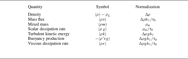
 $\rho _m(\rho _H,\rho _L)$
that we do not define explicitly at this point. Without further assumptions, we introduce the integrated mixed mass of the flow
 $M = \int \langle \rho m \rangle \,{\textrm {d}}y$
as an additional scaling parameter so that
 \begin{align} \langle \rho m \rangle \sim \frac {M}{h_1} \sim \rho _m. \end{align}
The normalization scale
 $M/h_1$
can be interpreted as a vertically averaged mixed mass, or a turbulent mixing density
 $\rho _m$
. Results will be presented first using
 $M/h_1$
scaling in this section; then, an a posteriori definition for
 $\rho _m$
will be proposed in § 5.1.
The effect of the Atwood number on the mixed mass is shown in figure 7(a,b), for the raw and normalized profiles, respectively. Since the mixed mass is normalized by its integral
 $M$
, the areas under the curves in figure 7(b) are identical by definition. After normalization, some Atwood number effects remain evident, which is reflected in a normalized spread of
 $\mathcal{E}_{\textit{rms}}\approx 0.12$
. Specifically, an increase in the Atwood number reduces the peak value of the mixed mass, shifts the peak to the left, and broadens the profiles. These effects are similar to the analytical 1-D solution discussed in Appendix B, where the equivalent 1-D mixed mass profile is shown. In § 4.1.1, we observed that the mean density field (represented by
 $\langle \rho \rangle$
,
 $\langle X \rangle$
or
 $\tilde {Y}$
) behaves in a similar manner to the 1-D solution. By extension, the mixed mass of the mean field,
 $\langle \rho \rangle \tilde {Y}(1-\tilde {Y})$
, would also resemble the mixed mass of the 1-D solution. The observations in figure 7(b) not only contain this expected result but further indicate that such quasi-1-D variable density effects on the mean field are also inherited by the second-order statistic,
 $\langle \rho m \rangle = \langle \rho Y(1-Y)\rangle$
.
Effect of the Atwood number on the (a) mixed mass, (b) normalized mixed mass, (c) scalar dissipation and (d) normalized scalar dissipation, based on
 $M/h_1$
scaling. Legend:
 $A=$
0.01 (magenta solid); 0.2 (blue dashed); 0.5 (red dash–dotted); 0.8 (green dotted).

The effect of the Reynolds number on the mixed mass are shown in figure 8(a,b). There are minor differences in the unnormalized mixed mass profiles in figure 8(a), possibly due to the small differences in
 $h_1/\mathcal{L}$
(see table 3). However, the normalized profiles in figure 8(b) are virtually identical (
 $\mathcal{E}_{\textit{rms}} \approx 0.02$
).
Effect of the Reynolds number on the (a) mixed mass (b) scalar dissipation, (c) normalized mixed mass and (d) normalized scalar dissipation. Legend:
 $Re\approx$
245 (red dotted); 496 (blue dash–dotted); 791 (magenta solid); 1060 (green dashed); 2540 (thick red solid); 4390 (thick black dashed).

The governing equation for the local mixed mass is derived by multiplying the scalar transport equation, (2.2), with
 $2Y$
and making simplifications using the continuity equation, (2.1). The ensemble-averaged mixed mass equation is
 \begin{align} 0 = - \frac {{\textrm {d}} \langle \rho v m \rangle }{{\textrm {d}}y} + \frac {{\textrm{d}}}{{\textrm {d}}y}\left \langle \rho D \frac {\partial m}{\partial y}\right \rangle + \langle \rho \chi \rangle +\frac {y}{\tau _0}\frac {{\textrm {d}} \langle \rho m \rangle }{{\textrm {d}}y}, \end{align}
where the terms correspond to convective transport, diffusive transport, scalar dissipation and the SRT source term, respectively. Neglecting the transport terms, a scaling for the dissipation rate can be derived from (4.13) and (4.14), yielding
 \begin{align} \langle \rho \chi \rangle \sim \frac {M}{h_1\tau _0}. \end{align}
The scalar dissipation rates for A0–A8 are presented in figure 7(c,d) for the raw and normalized profiles, respectively. Unlike the normalized mixed mass profiles of figure 7(b), the normalized peak values for scalar dissipation in figure 7(d) are similar across Atwood numbers, showing no discernible trend and agreeing to within
 $\pm 3\,\%$
. The leftward shift of the peak is more pronounced in the normalized scalar dissipation than in the normalized mixed mass. Compared with the equivalent profile for the analytical 1-D solution presented in Appendix B, this shift of the peak in SRT turbulence is quantitatively similar. However, unlike the 1-D solution, the maximum value of the scalar dissipation rate does not increase with Atwood number for SRT turbulence.
Finally, the effect of the Reynolds number on the scalar dissipation rate are presented in figure 8(c,d) for the raw and normalized profiles, respectively. Similar to observations on the viscous dissipation rate, Reynolds number effects are minimal after normalization, except in the less turbulent (i.e. lower
 $ \textit{Re} $
) cases. The overall spread of values is
 $\mathcal{E}_{\textit{rms}}\approx 0.05$
.
4.2. Scaling of global parameters
In § 4.1, scalings were proposed for the budget terms in terms of six global parameters, namely, the mixing layer height
 $h_1$
, gravity
 $g$
, time scale
 $\tau _0$
, the integrated mixed mass
 $M$
and the reservoir densities
 $\rho _H$
and
 $\rho _L$
. While
 $h_1$
,
 $g$
,
 $\rho _H$
and
 $\rho _L$
are input parameters,
 $\tau _0$
and
 $M$
are outputs of the SRT simulation. In this section, we relate
 $\tau _0$
and
 $M$
to the other parameters by using several simplifying assumptions, further reducing the total number of parameters required to the minimum set of
 $h_1$
,
 $g$
,
 $\rho _H$
and
 $\rho _L$
.
4.2.1. Mixing layer time scale
Consistent with the findings of TRT studies (Livescu et al. Reference Livescu, Ristorcelli, Gore, Dean, Cabot and Cook2009; Zhou & Cabot Reference Zhou and Cabot2019), we postulate that the TRT-equivalent growth of the SRT mixing layer scales with the magnitude of the turbulent velocity fluctuations such that
 \begin{align} \left( \frac{h_1}{\tau_0} \right)^2 \sim \tilde{k}, \end{align}
where the scaling for
 $\tilde {k}$
can be derived from previously established results. The Favre average is first written as
 \begin{align} \tilde {k} = \frac {\langle \rho k \rangle }{\langle \rho \rangle } = \frac {{\textrm {d}} \ln \langle \rho \rangle }{{\textrm {d}}\langle \rho \rangle } \langle \rho k \rangle = \frac {\langle \rho k \rangle }{{\textrm {d}}\langle \rho \rangle /{\textrm {d}} y}\frac {{\textrm {d}} \ln \langle \rho \rangle }{{\textrm {d}}y}. \end{align}
Then, to obtain a scaling relationship that is consistent with (4.1), two specific assumptions are invoked. First, the evolution of mean density is assumed to be diffusion-like, i.e.
 $\langle \rho \rangle$
and
 $\langle \rho v\rangle$
can be approximated by an error function (see figure 1
b) and Gaussian distribution (see figure 2
b), respectively. Second, the TKE profile
 $\langle \rho k \rangle$
inherits the shape of the mean mass flux through local buoyancy production scaling and can also be approximated as Gaussian (see figures 5, 6 and Appendix D). If
 $\langle \rho \rangle$
and
 $\langle \rho k \rangle$
were exact error and Gaussian functions, respectively, the ratio
 $\langle \rho k\rangle /[{\textrm {d}}\langle \rho \rangle / {\textrm {d}}y]$
would be independent of
 $y$
and equal to the ratio of their integrals. Utilizing this property in an approximate sense, and substituting (4.4) and (4.12), the scaling for
 $\tilde {k}$
becomes
 \begin{align} \int \tilde {k}\, {\textrm{d}}\left (\frac {y}{h_1}\right ) = \int \frac {\langle \rho k \rangle }{{\textrm {d}}\langle \rho \rangle /{\textrm {d}} y} \frac {{\textrm {d}} \ln \langle \rho \rangle }{{\textrm {d}}y}\, {\textrm {d}}\left (\frac {y}{h_1}\right ) \approx \frac {1}{h_1}\frac {\int \langle \rho k \rangle {\textrm {d}}y}{\int {\textrm {d}} \langle \rho \rangle } \int {\textrm {d}}\ln \langle \rho \rangle \propto gh_1 \ln R \end{align}
or, equivalently,
 \begin{align} \tilde {k} \sim gh_1 \ln R. \end{align}
Combining (4.16) and (4.19), the SRT time scale
 $\tau _0$
can be related to
 $h_1$
,
 $g$
,
 $\rho _H$
and
 $\rho _L$
via
 \begin{align} {\tau _0} \sim \left ( \frac {h_1} {g \ln R}\right )^{1/2}. \end{align}
Verification of
 $\tau _0$
scaling as a function of the (a) Atwood number (A0–A8) and (b) Reynolds number (G1–G6). Legend: unnormalized
 $\tau _0$
(black crosses); normalized
 $\tau _0[(g \ln R)/h_1]^{1/2}$
(blue circles).

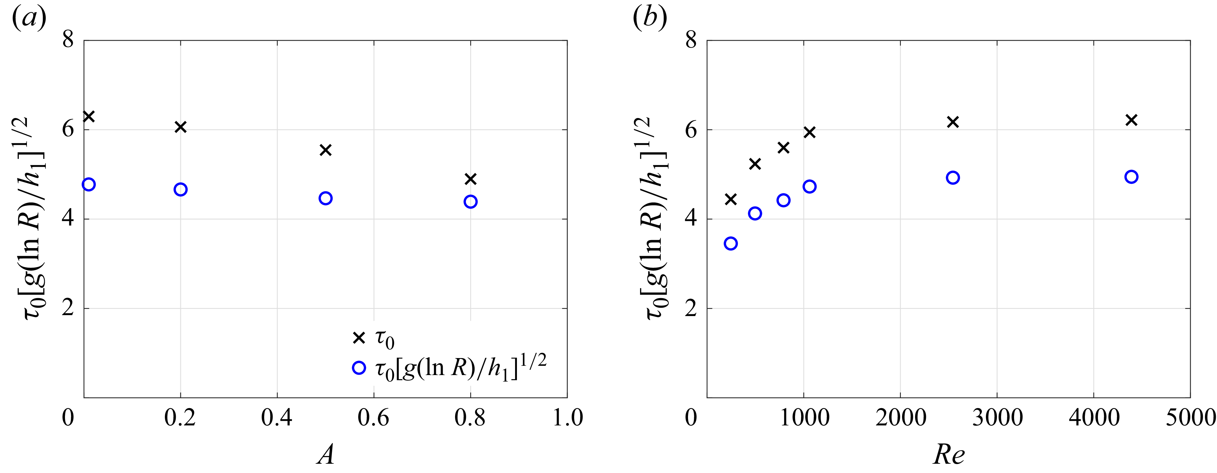
This scaling is evaluated using all simulation cases and presented in figures 9(a) and 9(b) for cases A0–A8 and G1–G6, respectively. In figure 9(a), the unnormalized values of
 $\tau _0$
decrease with increasing Atwood number. After normalization, they become approximately constant. In figure 9(b), the normalization has little effect on the Reynolds number trend. This is because
 $h_1$
,
 $g$
and
 $R$
are nearly constant across G1–G6. Nevertheless, the observed values of
 $\tau _0$
approach a high Reynolds number limit. The proposed scaling does not ‘correct’ for Reynolds number effects, because (4.16) assumes a sufficiently high Reynolds number regime where inertial effects dominate over viscous and diffusive processes. In the limiting case of pure 1-D diffusion (see Appendix B),
 $\tau _0 = \pi h_1^2/16D$
. Thus, it is reasonable to expect that
 $\tau _0$
may exhibit some dependence on
 $D$
(and
 $\nu$
) for low-Reynolds-number SRT turbulence. Despite this
 $ \textit{Re} $
-dependence of
 $\tau _0$
at low Reynolds numbers, we note that all profiles for cases G1–G6 shown in § 4.1 are almost identical after normalization, suggesting that the influence of the Reynolds number is almost entirely captured by the global parameter
 $\tau _0$
.
4.2.2. Integrated mixed mass
A scaling for the integrated mixed mass is developed in two main steps. First, the integrated mixed mass of the full SRT field,
 $M = \int \langle \rho Y(1-Y) \rangle \,{\textrm {d}}y$
, is related to the integrated mixed mass of the mean density field,
 $M_{\langle \rho \rangle } = \int \langle \rho \rangle \tilde {Y}(1-\tilde {Y})\,{\textrm {d}}y$
. Next, an estimate for
 $M_{\langle \rho \rangle }$
is proposed using a modelled mean mole fraction profile.
In § 4.1.3, it was observed that the average mixed mass,
 $\langle \rho Y(1-Y) \rangle$
, behaves similarly to the mixed mass of the mean density field,
 $\langle \rho \rangle \tilde {Y}(1-\tilde {Y})$
. To quantify the relationship between their integrals, a new measure of mixedness is introduced and defined as
 $\varTheta _m = M/M_{\langle \rho \rangle }$
. The values of
 $\varTheta _m$
for cases A0–A8 are shown in figure 10; they remain approximately constant at
 $\varTheta _m \approx 0.8$
. Hence, this ratio is modelled as a constant
 $\varTheta ^*_m$
, and any proposed scaling for
 $M_{\langle \rho \rangle }$
can be applied directly to
 $M$
.
Mixedness parameter
 $\varTheta _m= M/M_{\langle \rho \rangle }$
.

The next step is to establish a scaling relationship between
 $M_{\langle \rho \rangle }$
and the input parameters. Since both
 $\langle \rho \rangle$
and
 $\tilde {Y}$
are fully determined by the mean mole fraction
 $\langle X \rangle$
and the reservoir densities, so is the derived integral
 \begin{align} M_{\langle \rho \rangle } = \int \langle \rho \rangle \tilde {Y} (1-\tilde {Y}) \,{\textrm {d}}y = \frac {h_1}{4} \frac {\int \langle \rho \rangle \tilde {Y} (1-\tilde {Y}) \,{\textrm {d}}y}{\int \langle X\rangle (1-\langle X\rangle ) \,{\textrm {d}}y} = \frac {\rho _H h_1}{4} \frac {\int \frac {\langle X\rangle (1-\langle X\rangle )}{1+(R-1)\langle X\rangle }\,{\textrm {d}}y}{\int \langle X\rangle (1-\langle X\rangle ) \,{\textrm {d}}y}. \end{align}
To estimate
 $M_{\langle \rho \rangle }(\langle X \rangle , \rho _H, \rho _L)$
a priori, a model expression for the mean mole fraction
 $\langle X \rangle ^*$
is necessary, where the
 $^*$
superscript denotes a modelled quantity. In § 4.1.1, it was observed that the mean mole fraction does not change significantly with Atwood number and is well-approximated by the 1-D solution. Thus, the 1-D solution (derived in Appendix B) can be adopted as a model for the mean mole fraction,
 \begin{align} \langle X \rangle ^* = \frac {1}{2} \left [1 + \textrm {erf}\left ( \sqrt {\frac {8}{\pi }}\frac {y}{h_1} \right )\right ]\!, \end{align}
where the mixing layer height is matched, i.e.
 $h_1 = 4\int \langle X\rangle ^*(1-\langle X\rangle ^*)\,{\textrm {d}}y$
. Once
 $\langle X \rangle ^*$
is specified, the integrated mixed mass of the modelled mean density,
 $M^*_{\langle \rho \rangle }(\langle X\rangle ^*,\rho _H,\rho _L)$
, is obtained by substitution of
 $\langle X\rangle = \langle X\rangle^*$
in (4.21).
Combining the two steps, the integrated mixed mass
 $M$
can be expressed as
 \begin{align} M \approx \varTheta ^*_m M_{\langle \rho \rangle }(\langle X\rangle ,\rho _H,\rho _L) \approx \varTheta _m^* M^*_{\langle \rho \rangle }(\langle X\rangle ^*,\rho _H,\rho _L), \end{align}
where the right-hand side of (4.23) is solely a function of
 $\rho _H$
and
 $\rho _L$
.
5. Discussion
This section presents three extensions to the analysis of § 4. First, a reference density scale is inferred from the scaling of the integrated mixed mass. Second, normalized Favre-averaged velocity statistics are examined. Finally, a variable-density scaling law for the self-similar growth rate is derived and compared with the commonly used scaling expression (1.5) in the literature.
5.1. Density scale for the mixed mass
As discussed in § 4.1.3, the integrated mixed mass
 $M$
is expected to scale with the product of a mixing density
 $\rho _m$
and the height
 $h_1$
. Leveraging the observation that
 $\varTheta _m$
is approximately constant, we define
 \begin{align} \rho _m(\langle X\rangle ,\rho _H,\rho _L) = \rho _H \frac {\int \frac {\langle X\rangle (1-\langle X\rangle )}{1+(R-1)\langle X\rangle }\,{\textrm {d}}y}{\int \langle X\rangle (1-\langle X\rangle ) \,{\textrm {d}}y}, \end{align}
such that (4.21) is expressed as
 $M_{\langle \rho \rangle } = \rho _m h_1/4$
. Values of
 $\rho _m$
are extracted from cases A0–A8 and shown in figure 11, alongside several common averages of the reservoir densities: the arithmetic mean
 $\rho _a = (\rho _H+\rho _L)/2$
, geometric mean
 $\rho _g = \sqrt {\rho _H \rho _L}$
and harmonic mean
 $\rho _0=2/(\rho _H^{-1}+\rho _L^{-1})$
. The extracted SRT values of
 $\rho _m$
are significantly different from any of these simple averages considered.
Density scale for the mixed mass. Mean definitions of the reservoir densities are shown without markers: arithmetic mean
 $\rho _a$
(blue solid); geometric mean
 $\rho _g$
(green dash–dotted); harmonic mean
 $\rho _0$
(magenta dashed); SRT data
 $\rho _m = 4M_{\langle \rho \rangle }/h_1$
is represented by red filled markers; density scales derived from modelled expressions
 $\langle X \rangle ^*$
are shown as black dotted lines with markers: triangles (error function/1-D solution); squares (piecewise linear); circles (SRT mean mole fraction for case A0).

Extending the analysis of § 4.2.2, modelled mole fraction profiles can be applied to (5.1) to obtain possible models for the mixing density
 $\rho _m^*(\langle X\rangle ^*,\rho _H,\rho _L)$
. The error function solution proposed in (4.22) is an obvious candidate, but it is also possible to use alternative expressions for
 $\langle X \rangle ^*$
. To assess the sensitivity of
 $\rho _m^*$
to the assumed profile, three models are considered: the analytical 1-D solution (error function), a piecewise linear approximation and the mean mole fraction from the Boussinesq SRT case (A0). All three models perform noticeably better than any of the simple averages, which highlights the importance of accounting for the shape of the mole fraction profile. Among them, the error function yields the best agreement with the SRT data.
Finally, the definition of the mixing height
 $h_m$
used in Goh & Blanquart (Reference Goh and Blanquart2025) is revisited. Starting with its definition in (2.11), the mixing height
 $h_m$
can be related to
 $h_1$
using (4.21) and (5.1) such that
 \begin{align} h_m = \frac {4M}{\rho _0} = \varTheta _m \frac {4M_{\langle \rho \rangle }}{\rho _0} = \varTheta _m \frac {\rho _m}{\rho _0} \frac {4M_{\langle \rho \rangle }}{\rho _m} = \varTheta _m \frac {\rho _m}{\rho _0} h_1. \end{align}
The concerns highlighted in § 2.3 about the use of the harmonic mean as an arbitrary density normalization are illustrated by (5.2). While
 $\varTheta _m$
is approximately constant across Atwood numbers (see figure 10),
 $\rho _m/\rho _0$
is not (see figure 11). Proportionality of the large length scales is a feature of self-similar flows, but the existing definition of
 $h_m$
does not preserve similarity across Atwood numbers. A more physically appropriate definition of
 $h_m$
is
 \begin{align} h_{m,{ {new}}} = \frac {4M}{\rho _m^*} = \frac {4}{\rho _m^*}\int \langle \rho Y (1-Y)\rangle \,{\textrm {d}}y , \end{align}
where
 $\rho _m^*(\langle X \rangle ^*, \rho _H,\rho _L)$
is computed based on the model mole fraction profile described by (4.22).
5.2. Favre-averaged velocity statistics
In § 1, the scaling of velocity statistics was mentioned as an open question in the study of variable-density RT flows. In § 4, the scaling of the conserved variables
 $\langle \rho \phi \rangle$
were addressed, where
 $\phi$
represents
 $v$
,
 $k$
or
 $\epsilon$
. Here, we build on the scalings developed in § 4 to consider the effect of the Atwood number on Favre-averaged velocity statistics.
In (4.19) of § 4.2.1, the scaling for
 $\tilde {k}$
was derived from
 $\langle \rho k\rangle$
by using the result
 ${\textrm {d}} \ln \langle \rho \rangle = {\textrm {d}}\langle \rho \rangle /\langle \rho \rangle$
, and approximating
 $\langle \rho k \rangle$
as a Gaussian function. Because the mean mass flux
 $\langle \rho v \rangle$
and viscous dissipation rate
 $\langle \rho \epsilon \rangle$
profiles have similar shapes to the TKE, the assumptions for the derivation of (4.19) are expected to be satisfied approximately. Hence, the same procedure is used to obtain scalings for
 $\tilde {v}$
and
 $\tilde {\epsilon }$
leveraging the scalings for
 $\langle \rho v \rangle$
and
 $\langle \rho \epsilon \rangle$
. The unnormalized Favre-averaged profiles are shown in figure 12(a,c,e), and the normalized profiles are shown in figure 12(b,d,f). There are three key observations.
Effect of the Atwood number on the (a) Favre-averaged velocity, (b) normalized Favre-averaged velocity, (c) Favre-averaged TKE, (d) normalized Favre-averaged TKE, (e) Favre-averaged viscous dissipation and (f) normalized Favre-averaged dissipation. Legend:
 $A=$
0.01 (magenta solid); 0.2 (blue dashed); 0.5 (red dash–dotted); 0.8 (green dotted).

First, the maximum values of the unnormalized quantities increase significantly with Atwood number, while those of the normalized profiles agree to within 5 %, demonstrating the effectiveness of the proposed
 $\ln R$
scaling for all velocity statistics considered.
Second, while the conserved quantities,
 $\langle \rho v \rangle$
,
 $\langle \rho k\rangle$
and
 $\langle \rho \epsilon \rangle$
, all have peak values at
 $y\approx 0$
, there is a leftward shift of the peaks for all Favre-averaged profiles as the Atwood number increases, similar to trends observed by Livescu et al. (Reference Livescu, Ristorcelli, Petersen and Gore2010). This is merely a consequence of dividing near-symmetric
 $\langle \rho \phi \rangle$
profiles by an asymmetric, monotonically increasing
 $\langle \rho \rangle$
profile. Dividing by smaller mean density values on the left of
 $y=0$
than on the right causes the shift. This effect is not dissimilar to the leftward shift of the Favre-averaged mass fraction profiles shown in figure 1 and is also evident in the normalized velocity of the 1-D diffusion solution presented in Appendix B.
Third, the apparent shift of the peaks has implications on the interpretation of turbulence statistics. For instance, the Kolmogorov scale is commonly defined in variable density flows using the Favre-averaged dissipation,
 $\eta = (\nu ^3/\tilde {\epsilon })^{1/4}$
. In figure 12(f), the location of the smallest turbulence scales (i.e. maximum dissipation) shifts towards the light-fluid side as the Atwood number increases. Based on this definition of
 $\eta$
, the smallest scales are not found at
 $y=0$
, even though this is commonly assumed to be the ‘core’ of the mixing layer. Any comparison of small-scale statistics across different Atwood numbers should take this shift into consideration.
5.3. Effective Atwood number for non-Boussinesq flows
The final discussion addresses the scaling of the growth rate for variable-density RT flows, conventionally represented by (1.5). Figure 13(a) shows the growth rate parameter
 $\alpha _1$
extracted from two separate sources. First, it is evaluated from SRT cases A0–A8 using the equivalent definition
 $\alpha _1 = h_1/(4Ag\tau _0^2)$
. Second, the range of
 $\alpha _p$
values from the TRT simulations of Zhou & Cabot (Reference Zhou and Cabot2019) (summarized in table 4) are converted to
 $\alpha _1$
using
 $h_1/h_{\kern-1pt p}$
ratios derived from the SRT data. Both sets of data indicate that
 $\alpha _1$
increases with the Atwood number, consistent with observations from experimental studies (Dimonte & Schneider Reference Dimonte and Schneider2000; Banerjee et al. Reference Banerjee, Kraft and Andrews2010). The observed
 $\alpha _1(A)$
trend is a direct consequence of the scaling of
 $\tau _0$
presented in (4.20).
Equation (1.5) was derived using the Boussinesq approximation (Ristorcelli & Clark Reference Ristorcelli and Clark2004). For variable-density flows, (1.5) can be generalized as
 \begin{align} \dot {h}_i^2 = 4F_i(A)gh_i, \end{align}
where
 $F_i(A) = \alpha _i(A)A$
. Building on the demonstrated scaling of (4.20), we seek an alternative expression for
 $F_i$
that accounts for variable-density effects using a modified or effective Atwood number. Specifically, we propose the form
 $F_i(A) = \alpha _i^*A^*(A)$
, where all density effects are captured by the effective Atwood number
 $A^*$
and
 $\alpha _i^*$
is a universal constant that is truly independent of
 $A$
. The functional form of
 $A^*(A)$
is derived below.
(a) Standard growth parameter
 $\alpha _1$
and (b) effective growth parameter
 $\alpha _1^*$
. Legend: SRT results (markers); range of TRT values from Zhou & Cabot (Reference Zhou and Cabot2019) (bars); constant-
 $\alpha _1^*$
model (dotted line).

Rearranging (4.20), squaring both sides and including a constant of proportionality
 $4\alpha _1^*C$
yields
 \begin{align} \left (\frac {h_1}{\tau _0}\right )^2 \approx 4\alpha _1^* C g h_1 \ln R, \end{align}
which has a
 $\ln R$
dependence that is consistent with (1.6) proposed by Belen’kii & Fradkin (Reference Belen’kii and Fradkin1965) – a similarity that will be discussed in § 5.4. To maintain consistency of the
 $\ln R$
scaling with the large number of studies done in the Boussinesq limit, the constant of proportionality
 $4\alpha _1^*C$
is included and
 $C$
is chosen such that
 $\alpha _i^*(\Delta \rho \to 0) = \alpha _i(\Delta \rho \to 0)$
. The right-hand side of (1.5) is evaluated for
 $h_i=h_1$
and expanded in a Taylor series as
 \begin{align} 4\alpha _1 A g h_1 = 4\alpha _1 g h_1 \left [ \frac {1}{2}\left (\frac {\Delta \rho }{\rho _L}\right ) - \frac {1}{4}\left (\frac {\Delta \rho }{\rho _L}\right )^2 + \frac {1}{8}\left (\frac {\Delta \rho }{\rho _L} \right )^3 + \ldots \right ]\!, \end{align}
while the corresponding expansion for the right-hand side of (5.5) is
 \begin{align} 4\alpha _1^*Cgh_1 \ln R = 4\alpha _1^* g h_1 C\left [ \left (\frac {\Delta \rho }{\rho _L}\right ) - \frac {1}{2} \left (\frac {\Delta \rho }{\rho _L}\right )^2 + \frac {1}{3} \left (\frac {\Delta \rho }{\rho _L} \right )^3 - \ldots \ \right ]\!. \end{align}
Applying the constraint
 $\alpha _1^*(\Delta \rho \to 0) = \alpha _1(\Delta \rho \to 0)$
and matching the leading-order terms, we find
 $C=1/2$
. Hence, (5.5) can be used to define an effective Atwood number,
 \begin{align} A^* = \frac {1}{2}\ln R, \end{align}
such that
 \begin{align} \left ( \frac {h_1}{\tau _0}\right )^2 = 2\alpha _1^*gh_1 \ln R = 4\alpha _1^* A^* g h_1. \end{align}
The effective Atwood number
 $A^*$
is equal to
 $A$
in the Boussinesq limit but differs significantly at higher Atwood numbers, as shown in figure 14(a). Rearranging (5.9), the effective growth parameter
 $\alpha _1^*$
is computed using
 $\alpha ^*_1 = h_1/(4 A^*g\tau _0^2)$
and shown in figure 13(b). As intended,
 $\alpha _1^*=\alpha _1$
for small Atwood numbers. For the SRT cases considered, the variation in
 $\alpha ^*_1$
is 70 % smaller than that of
 $\alpha _1$
, with a near-universal value of
 $\alpha ^*\approx 0.024$
. This suggests that
 $A^*$
is a more complete representation of the density effects associated with a variable-density RT flow. The constant-
 $\alpha _1^*$
model can explain the Atwood number trends of
 $\alpha _1$
using
 $\alpha _1 = \alpha _1^*A^*/A \approx 0.024A^*/A$
. This estimate is included in figure 13(a), which shows a good agreement with both SRT and TRT data.
(a) Effective Atwood number
 $A^*$
with respect to
 $A$
, and (b) comparison of Grashof number definitions using SRT cases A0–A8. Legend: standard
 $ \textit{Gr}$
(black markers); effective
 $Gr^*$
(blue circles).

In addition to the DNS results, the scaling based on the effective Atwood number is validated against previous experiments (Dimonte & Schneider Reference Dimonte and Schneider2000; Banerjee et al. Reference Banerjee, Kraft and Andrews2010) and large-eddy simulations (Youngs Reference Youngs2013). The comparison is limited to studies that explored a range of Atwood numbers within a single experimental or computational set-up. In all three studies, a growth parameter representative of the full mixing layer is computed as the mean of the reported bubble (
 $\alpha _b$
) and spike (
 $\alpha _s$
) growth parameters, although each study used different definitions for the bubble and spike heights. These averaged
 $\alpha _i$
values are presented in figure 15(a). It is important to note that, due to differences in initial conditions and height definitions, the absolute values of
 $\alpha _i$
are not expected to be consistent between studies. Nevertheless,
 $\alpha _i$
consistently increases with Atwood number for all cases. To explore the validity of
 $A^*$
scaling, the standard growth parameters are converted to effective growth parameters using
 $\alpha _i^* = \alpha _iA/A^*$
and shown in figure 15(b). Within each study, the values remain approximately constant across the range of Atwood numbers, indicating that the effective Atwood number successfully normalizes the growth behaviour. The results also suggest that the scaling relationships developed based on DNS data for
 $A\leqslant 0.8$
remain valid under conditions beyond this range.
(a) Standard growth parameter
 $\alpha _i$
and (b) effective growth parameter
 $\alpha _i^*$
extracted from other RT studies of Atwood number effects. Legend: Dimonte & Schneider (Reference Dimonte and Schneider2000) (green circles); Banerjee et al. (Reference Banerjee, Kraft and Andrews2010) (red squares); Youngs (Reference Youngs2013) (blue triangles). Initial conditions and height definitions vary across studies. Here LES stands for large-eddy simulations.

The Atwood number also appears in the definition of the Grashof number, as shown in (2.14). In § 3.1, it was described that the input Grashof number in table 2 was reduced at higher Atwood numbers in order to maintain a constant Reynolds number (or
 $h_1/\eta$
). This difference in trends between
 $ \textit{Gr}$
and
 $ \textit{Re} $
can be explained by substituting (5.9) into the definition of the Reynolds number,
 \begin{align} Re^2 = \frac {h_1^4}{\tau _0^2\nu ^2} = 4\alpha ^* \frac {A^*gh_1^3}{\nu ^2} = 4\alpha ^*Gr^*, \end{align}
where
 $Gr^*$
has an identical definition to
 $ \textit{Gr}$
, except for the replacement of
 $A$
with
 $A^*$
. It is
 $Gr^*$
(and not
 $ \textit{Gr}$
) that scales with
 $Re^2$
. Both definitions of the Grashof number are shown in figure 14(b) for the Atwood number sweep of A0–A8 at constant Reynolds number. Indeed,
 $Gr^*$
has an approximately constant value.
5.4. Summary of scaling relationships and physical insights
To offer the reader a comprehensive overview of the results, this concluding discussion summarizes the derived scaling relations and highlights the key physical assumptions underlying their derivation.
The scaling of the budget terms derived in § 4.1 is summarized in table 5. The mixed mass budget was normalized by a vertically averaged mixed mass
 $M/h_1$
, or a turbulent mixing density
 $\rho _m$
, while the TKE budget was normalized by the total potential energy loss of the flow
 $\Delta \rho g h_1$
. Both sets of scalings retained the SRT time scale parameter
 $\tau _0$
. To achieve a true self-similar scaling (where all dynamical properties of the flow depend solely on
 $h_1$
),
 $\tau _0$
and
 $\rho _m$
were related to the input variables (
 $\rho _H$
,
 $\rho _L$
,
 $g$
,
 $h_1$
) in § 4.2 based on the following physical observations on RT turbulence.
Summary of scalings.

-
(i) The mean mole fraction profile resembles that of a 1-D diffusion problem: this determines the shape of the mean mass flux and the buoyancy production term in the TKE budget.
-
(ii) The integrated mixing parameter (as defined by
$\varTheta _m$
) is independent of Atwood number. Combined with (i), an (approximate) equivalence is established between the turbulent mixing density
$\rho _m$
and the diffusion mixing density
$\rho _m^*$
, which has an analytical solution based solely on
$\rho _H$
and
$\rho _L$
. -
(iii) The growth rate of the mixing layer
$h/\tau _0$
is related to the turbulent velocity fluctuations
$\tilde {k}^{1/2}$
(and not the mean velocity
$\tilde {v}$
). -
(iv) The conserved form of the TKE
$\langle \rho k\rangle$
scales with buoyancy production locally (at each
$y$
location) and not just in a volume-integrated sense. As a result, the TKE profile preserves the Gaussian-like shape of the mean mass flux, which is similar to the gradient of the mean density. Combined with an algebraic ‘trick’ that writes
$1/\langle \rho \rangle$
as
${\textrm {d}}\ln \langle \rho \rangle /{\textrm {d}}\langle \rho \rangle$
, the scaling for
$\tau _0$
is derived.


Other trends observed in this study can be related back to these four observations. First, the derivation of the effective Atwood number (and effective Grashof number) is simply an algebraic consequence of the scaling of
 $\tau _0$
. Second, observation (i) implies an invariance of the mole fraction
 $\langle X \rangle$
profile, which dictates (by definition) that Favre-averaged mass fraction
 $\tilde {Y}$
profiles are shifted towards the light-fluid side. The observed shifts in mass-fraction-based quantities like the mixed mass and scalar dissipation rate are also consistent with the diffusive description of RT turbulence. Third, the near-symmetric profiles of the TKE budget terms are a combined consequence of observations (i) and (iv) – their Favre-averaged profiles are shifted simply due to division by a monotonically increasing mean density.
As introduced in § 1 through (1.6), the scaling of the mixing layer height with
 $\ln R$
was first proposed in the theoretical analysis of Belen’kii & Fradkin (Reference Belen’kii and Fradkin1965), based on a combination of energy scaling arguments and a spatially varying turbulent diffusivity model. Although derived independently, the consistency in our results is unsurprising, as the analysis of Belen’kii & Fradkin (Reference Belen’kii and Fradkin1965) relied on the same physical assumptions (i) and (iv), which had not been verified with physical data until the present study. In Belen’kii & Fradkin (Reference Belen’kii and Fradkin1965), these assumptions led to the definition of a self-similar problem for the mean density, which, when constrained to small density ratios (
 $R\lesssim 4$
), has an exact solution that includes
 $\ln R$
. In the present work, the mean mole fraction is approximated by an error function, which leads to the same scaling. To our knowledge, this work provides the first verification of the
 $\ln R$
scaling using RT data. Furthermore, we demonstrate that the
 $\ln R$
scaling remains effective for density ratios well beyond the range initially constrained by Belen’kii & Fradkin (Reference Belen’kii and Fradkin1965).
The mean density profile determines the shape of the mean mass flux, buoyancy production and TKE; it also drives the shift in Favre-averaged profiles towards the light-fluid side. In the present work, approximating the mean mole fraction with an error function proved effective for estimating integrated normalization quantities. However, improving the mean density model could enhance predictions for other profile quantities. Boffetta, De Lillo & Musacchio (Reference Boffetta, De Lillo and Musacchio2010) proposed a turbulent diffusivity closure similar to Belen’kii & Fradkin (Reference Belen’kii and Fradkin1965) that was validated with DNS results of Boussinesq RT turbulence. Extending such models to the general variable-density case could lead to a more complete description of RT turbulence.
6. Conclusion
The present work extends the methodology of Goh & Blanquart (Reference Goh and Blanquart2025) to a range of Atwood numbers,
 $A\leqslant 0.8$
. The SRT MFU at
 $\lambda = 1.7$
is used as a surrogate for self-similar TRT flows, for which highly converged statistics were obtained across a broad range of Atwood and Reynolds numbers. Normalizations were developed for all significant non-transport terms in the continuity, mixed mass and TKE budgets. When applied to the SRT data, most quantities exhibit strong collapse in their profiles after normalization. In some cases, the normalized profiles shift towards the light-fluid side with increasing Atwood number, matching trends observed in the 1-D variable-density diffusion solution.
For the SRT MFU, the mixing layer height is found to scale with
 $\ln R$
, a scaling originally proposed by Belen’kii & Fradkin (Reference Belen’kii and Fradkin1965), but which has not been applied in subsequent RT studies. An effective Atwood number is introduced as
 $A^*=(\ln R)/2$
, which reduces to the standard Atwood number in the Boussinesq limit. Applying this scaling to TRT results, the corresponding effective growth parameter,
 $\alpha ^*=\dot {h}^2/4A^*gh$
, exhibits a significantly reduced dependence on the Atwood number compared with the traditional growth parameter
 $\alpha$
. Further, defining the Grashof number using
 $A^*$
yields an effective Grashof number
 $Gr^*$
that scales directly with
 $Re^2$
, reinforcing the internal consistency of the proposed scaling.
The observed universality of the normalized quantities presents opportunities for broader application. In particular, Reynolds number effects in SRT turbulence appear to be almost entirely captured by the mixing layer growth time scale (or equivalently,
 $\alpha ^*$
). The influence of the Atwood number on the integrated quantities is largely reflected in the proposed scalings, while possible shifts in the profiles can be predicted using the 1-D analytical solution. These observations highlight the potential for using lower-cost DNS studies of low-Reynolds-number Boussinesq RT flows to estimate flow statistics under more extreme conditions.
Acknowledgements
This work used resources provided by Texas Advanced Computing Center (TACC), The University of Texas at Austin through allocation MCH230009 from the Advanced Cyberinfrastructure Coordination Ecosystem: Services & Support (ACCESS) program (Boerner et al. Reference Boerner, Deems, Furlani, Knuth and Towns2023), which is supported by U.S. National Science Foundation grants #2138259, #2138286, #2138307, #2137603 and #2138296. This work also used resources of the National Energy Research Scientific Computing Center, a DOE Office of Science User Facility supported by the Office of Science of the US Department of Energy under Contract No. DE-AC02-05CH11231 using NERSC award FES-ERCAP0031321. Additionally, the authors acknowledge the use of Google AI to assist in translating the original document of Belen’kii & Fradkin (Reference Belen’kii and Fradkin1965) from Russian into English.
Funding
This material is based upon work supported by the National Science Foundation under grant no. 2422513.
Declaration of interests
The authors report no conflict of interest.
Appendix A. Impact of the SRT source terms on energy spectra
The impact of the SRT source terms, (2.6)–(2.7), on the energy spectra is examined. Combining (2.1) and (2.3), the momentum equation can be written as
 \begin{align} \frac {\partial u_i}{\partial s} = -u_{\kern-1.5pt j}\frac {\partial u_i}{\partial x_{\kern-1.5pt j}} - \frac {1}{\rho }\left (\frac {\partial p}{\partial x_i} - \frac {\partial \tau _{\textit{ij}}}{\partial x_{\kern-1.5pt j}}\right ) + \frac {y}{\tau _0}\frac {\partial u_i}{\partial y} - \frac {u_i}{2\tau _0}. \end{align}
Applying a Fourier transform (notated as
 $\mathcal{F}$
) to (A1) in the homogeneous directions (
 $x_1$
,
 $x_3$
) yields
 \begin{align} \frac {\partial \hat {u}_i}{\partial s} = \mathcal{F}\left [-u_{\kern-1.5pt j}\frac {\partial u_i}{\partial x_{\kern-1.5pt j}} - \frac {1}{\rho }\left (\frac {\partial p}{\partial x_i} - \frac {\partial \tau _{\textit{ij}}}{\partial x_{\kern-1.5pt j}}\right )\right ] + \frac {y}{\tau _0}\frac {\partial \hat {u}_i}{\partial y} - \frac {\hat {u}_i}{2\tau _0}, \end{align}
where
 $\hat {u}_i = \mathcal{F}(u_i)$
, and the in-plane Fourier transform commutes with the differential operator in
 $y$
. Then, (A2) is multiplied by
 $\hat {u}_i^*$
to derive an equation for the two-dimensional energy spectrum
 $\hat {E}(k_1,y,k_3,s) = (\hat {u}_i\hat {u}_i^*)/2$
. The result is
 \begin{align} \frac {\partial \hat {E}}{\partial s} = \hat {u}_i^*\boldsymbol{\cdot }\mathcal{F}\left [-u_{\kern-1.5pt j}\frac {\partial u_i}{\partial x_{\kern-1.5pt j}} - \frac {1}{\rho }\left (\frac {\partial p}{\partial x_i} - \frac {\partial \tau _{\textit{ij}}}{\partial x_{\kern-1.5pt j}}\right )\right ] + \frac {1}{\tau _0}\left (y\frac {\partial }{\partial y} - 1\right ) \hat {E}. \end{align}
Represented by the rightmost term in (A3), the source terms act proportionally to the in-plane TKE spectra, and do not selectively inject or remove energy in any specific wavenumber range. Graphically, the effect of the source terms corresponds to a continuous downward shift of the entire energy spectra (when displayed on a logarithmic scale).
Appendix B. Analytical solution to variable-density 1-D diffusion
The 1-D variable-density temporal diffusion problem in
 $(t,y)$
coordinates is entirely governed by continuity, scalar transport and the equation of state. They are
 \begin{align} \frac {\partial \rho }{\partial t} + \frac {\partial \rho v}{\partial y} &= 0, \\[-28pt] \nonumber \end{align}
 \begin{align} \frac {\partial \rho Y}{\partial t} + \frac {\partial \rho v Y}{\partial y} &= D\frac {\partial }{\partial y}\left (\rho \frac {\partial Y}{\partial y}\right )\!, \\[-28pt] \nonumber \end{align}
 \begin{align} \rho (Y) &= \frac {\rho _H \rho _L}{\rho _H- Y\Delta \rho }. \\[-2pt] \nonumber \end{align}
Equations (B1)–(B3) determine
 $\rho$
,
 $v$
and
 $Y$
completely. The solution is diffusion driven and does not depend on gravity. With
 $\rho$
and
 $v$
determined, the pressure can be obtained from the momentum equation using known values of
 $g$
and
 $\nu$
.
The analytical self-similar solution to the variable-density diffusion problem, expressed in terms of the similarity variable,
 $\zeta = y/\sqrt {4Dt} = y/h_D$
(notated with subscript
 $D$
for ‘diffusion’) is
 \begin{align} X = \frac {\rho -\rho _L}{\Delta \rho } &= \frac {1}{2}(1 + \textrm{erf}\, \zeta ), \\[-28pt] \nonumber \end{align}
 \begin{align} \frac {\rho v}{\Delta \rho D/h_D} &= -\frac {{\textrm {d}} X}{{\textrm {d}}\zeta } = -\frac {1}{\sqrt {\pi }} e^{-\zeta ^2}, \\[-2pt] \nonumber \end{align}
where the solution for the mole fraction is identical to that of the constant-density problem, and variable-density effects are only observed in the velocity. The mole fraction
 $X$
is solely a function of
 $\zeta$
and independent of the reservoir densities. In contrast, the mass fraction
 $Y$
, which is algebraically related to
 $X$
by the equation of state,
 $Y(X, R) = RX/[1 + (1-R)X]$
, does vary with the density ratio (i.e. Atwood number). By extension, this is generally true for all functions of
 $Y$
, including the 1-D mixed mass,
 $m=\rho Y(1-Y)$
, and scalar dissipation rate,
 $\chi = 2\rho D(\partial Y/\partial y)^2$
, as shown in figure 16. For ease of comparison with the SRT results, quantities in figure 16 are normalized with the equivalent variables, where
 $h_1 = \sqrt {8/\pi } h_D$
,
 $M = \int \rho m \,{\textrm {d}}y$
and
 $\tau _0 = h_D/\dot {h}_D = h_D^2/2D = \pi h_1^2/16D$
. As
 $A$
increases, the mass fraction and velocity shifts leftwards, the mixed mass profile broadens with a reduction in its peak value and the scalar dissipation narrows while experiencing an increase in its peak value.
Analytical solution to the 1-D variable-density diffusion problem in normalized variables: (a) mole fraction (independent of
 $A$
); (b) mass flux (independent of
 $A$
); (c) mass fraction; (d) velocity; (e) mixed mass; (f) scalar dissipation rate. Legend:
 $A=0$
(thick black solid); 0.2 (thick blue dashed); 0.5 (red dash–dotted); 0.8 (green dotted); 0.95 (cyan solid); 0.99 (magenta dashed).

Appendix C. Closure equation for
$h_1$

To derive a time evolution equation for the instantaneous mixing layer height
 $h_1(s)$
, density is written in terms of the mole fraction,
 $\rho = \rho _L + \Delta \rho X$
, and substituted into the continuity equation to yield
 \begin{align} \frac {\partial \langle X \rangle _{1,3}}{\partial s} + \frac {1}{\Delta \rho }\frac {\partial \langle \rho v \rangle _{1,3}}{\partial y} = \frac {y}{\tau _0} \frac {\partial \langle X \rangle _{1,3}}{\partial y}. \end{align}
An equation for the transport of
 $\langle X \rangle _{1,3}^2$
is obtained by multiplying (C1) with
 $2\langle X \rangle _{1,3}$
to get
 \begin{align} \frac {\partial \langle X \rangle _{1,3}^2}{\partial s} + \frac {2}{\Delta \rho } \langle X \rangle _{1,3} \frac {\partial \langle \rho v\rangle _{1,3}}{\partial y} = \frac {y}{\tau _0}\frac {\partial \langle X \rangle _{1,3}^2}{\partial y}. \end{align}
Combining (C1) and (C2) results in
 \begin{align} \frac {{\textrm {d}} h_1}{{\textrm {d}}s} = \frac {{\textrm {d}}}{{\textrm {d}}s} \int 4\big (\langle X \rangle _{1,3} - \langle X \rangle _{1,3}^2\big )\,{\textrm {d}}y= \frac {8}{\Delta \rho }\int \langle X \rangle _{1,3} \frac {\partial \langle \rho v \rangle _{1,3}}{\partial y} \,{\textrm {d}}y- \frac {h_1}{\tau _0}. \end{align}
The SRT parameter
 $\tau _0$
is implemented by assuming a steady solution,
 ${\textrm {d}}h_1/{\textrm {d}}s=0$
, to (C3) and substituting
 $h_1 = \hat {h}_1$
so that
 \begin{align} \frac {1}{\tau _0(s)} = \frac {8}{\Delta \rho \hat {h}_1} \int \langle X \rangle _{1,3} \frac {\partial \langle \rho v \rangle _{1,3}}{\partial y} \,{\textrm {d}}y. \end{align}
Substituting (C4) into (C3) results in a time evolution equation for
 $h_1$
that is written as
 \begin{align} \frac {{\textrm {d}} h_1}{{\textrm {d}}s} = \frac {{\textrm {d}}}{{\textrm {d}}s} \int 4 \langle X \rangle _{1,3} \left (1- \langle X \rangle _{1,3}\right ){\textrm {d}}y= \left [\frac {8}{\Delta \rho }\int \langle X \rangle _{1,3} \frac {\partial \langle \rho v \rangle _{1,3}}{\partial y} \,{\textrm {d}}y\right ] \left (1 - \frac {h_1}{\hat {h}_1}\right )\!. \end{align}
The integral factor in the right-hand side of (C5) is positive for an unstable RT flow configuration, hence the use of (C4) results in a stable relaxation equation for
 $h_1$
. The use of closure equations such as (2.8) or (C4) (as opposed to a constant
 $\tau _0$
) is simply a practical way of achieving a specified mixing layer height without the need to guess the value of
 $\tau _0$
a priori. It was shown in Appendix A of Goh & Blanquart (Reference Goh and Blanquart2025) that the ensemble dynamics of SRT flow is equivalent for different implementations of
 $\tau _0$
as long as the value of the time average
 $\bar {\tau }_0$
is the same.
Appendix D. Local scaling of TKE with buoyancy production
A qualitative observation about the TKE budget profiles in figures 5 and 6 is that buoyancy production and TKE profiles have similar shapes that resemble a Gaussian function. To assess their similarities more quantitatively, buoyancy production is normalized by TKE and shown in figure 17. Towards the edge of the mixing layer, both buoyancy production and TKE approach zero, and the division of small values may lead to significant noise. To focus on the behaviour of the bulk of the mixing layer, only regions where buoyancy production is at least 10 % of its maximum value are shown.
The ratio of buoyancy production to TKE growth is remarkably constant across the mixing layer at around 2.2, which suggests that the buoyancy production scaling applies not only globally, but also locally, and that the TKE profile largely preserves the shape of buoyancy production (and by extension, the mean mass flux). This local scaling of TKE with buoyancy production is a key observation that is utilized in the derivation of the scaling for
 $\tau _0$
in § 4.2.
Ratio of buoyancy production to TKE growth. Atwood number effects are represented by
 $A=$
0.01 (magenta solid), 0.2 (blue dashed), 0.5 (red dash–dotted), 0.8 (green dotted); and Reynolds number effects are represented by dash–dotted lines of different shades of red. Only regions where buoyancy production is at least 10 % of its maximum value are shown with full opacity.