


“I decided rather than terminating NAFTA. . .we will renegotiate. Now, if I’m unable to make a fair deal, if I’m unable to make a fair deal for the United States, meaning a fair deal for our workers and our companies, I will terminate NAFTA. But we’re going to give renegotiation a good, strong shot.”
President Trump, April 27, 2017
INTRODUCTION
States sign treaties, accede to international institutions and organizations, and lend money to other states. The division of the surplus arising from these activities is negotiated by the governments of the day. However, these governments may, in turn, be replaced by new governments over the life of the agreement. This raises the possibility that arrangements signed by today’s administrations may not be honored by their successors.
In fact, newly elected governments often try to renegotiate a predecessor’s agreement. A Conservative government took the United Kingdom into the European Economic Community (EEC) in 1973. That same year, the Labour Party declared that it “opposes British membership [in the EEC] on the terms negotiated by the Conservative Government,” and its 1974 election manifesto promised to “seek a fundamental re-negotiation.”Footnote 1 Upon entering government in 1974, Labour reopened negotiations, obtaining concessions in exchange for the UK’s continued participation. After the 2015 general election, a Conservative government initiated the renegotiation that culminated in a vote for the UK to exit the European Union (“Brexit’’). In May 2017, the Trump administration notified Congress that it plans to renegotiate the North American Free Trade Agreement (NAFTA). And in June 2017, Donald Trump withdrew the United States from the Paris Climate accord with the prime intent to renegotiate better terms, asserting:
“In order to fulfill my solemn duty to protect America and its citizens, the United States will withdraw from the Paris climate accord but begin negotiations to reenter either the Paris accord or an entirely new transaction on terms that are fair to the United States.”
International negotiations may polarize and even dominate domestic politics. In March 2010, the European Central Bank, EU, and IMF (the “Troika’’) established emergency loan agreements to Greece. The first Greek bailout was negotiated between the Troika and the center-left PASOK government, which held a parliamentary majority of fewer than ten seats and hence faced an ongoing threat of electoral replacement over the life of the agreement. A domestic power transition to an anti-bailout party could threaten the agreement’s survival and the perceived harshness of the initial terms could itself increase the chance of a more hostile future government via voters’ dissatisfaction with the agreement. Both risks were realized: in the next election, PASOK lost 119 seats, while Syriza—the radical left-wing party that staunchly opposed the bailout terms—became the second largest party. In January 2015, Syriza came to power on the back of the Greek electorate’s hostility to the austerity measures. The new Greek government immediately reopened negotiations with EU member states, which nearly led Greece to exit the European Monetary Union.
In the context of a renegotiation, the effective bargaining power of a government typically derives from its relative willingness to walk away from an existing agreement, either in accordance with an exit process stipulated in the agreement itself, or by simply abrogating the terms.Footnote 2 This was manifest in the unilateral decision by the Bush Administration to withdraw from the Kyoto Protocol in 2001, and in 2017 when the Trump Administration threatened to “terminate” NAFTA absent a renegotiation that would deliver a “fair deal” for the United States.Footnote 3 Indeed, when Margaret Thatcher renegotiated a two-thirds rebate of Britain’s contribution to the budget of the EEC in 1984, she is reported to have succeeded only by threatening to withhold all of Britain’s contribution unless her demands were met.Footnote 4 The revised British contribution remained in place until 2005.Footnote 5
Our paper asks: How do pending national elections determine (a) the prospects for initial cooperation between states and (b) the division of the surplus from an agreement? And how do the terms of an initial agreement affect the prospect of electoral replacement, the bargaining attitude of a potential successor, or the risk that a successor will walk away from the agreement?
Our Approach. At each of two dates, a domestic government negotiates an agreement with a foreign government. The agreement specifies whether a binary policy project is undertaken and the extent of transfers to be made between governments in return for implementing the project. The transfers could include budget contributions, rebates, or regulatory carve-outs. Agents hold commonly known initial project valuations. The domestic incumbent is either intrinsically relatively friendly or hostile to the project, but we assume that neither domestic party initially wants to implement the project without some concessions from the foreign government.
After the initial negotiations conclude, a national election determines whether the incumbent is retained or replaced by the other party. We first assume that the uncertainty over who will hold power at date two is unaffected by date-one outcomes. We then assume that voters cast their ballots for whichever party is best for them given the agreement that was initially negotiated. Following elections, domestic agents receive a stochastic and publicly observed shock to their preferences over the project. For example, civil unrest may raise the domestic political cost of the project regardless of which political party holds power.
At date two, the transfer negotiated before the election serves as the transfer that would be made if the new domestic government again implements the project. However, either the foreign or domestic government may renegotiate the existing terms by proposing a new transfer. If accepted by the other government, the proposed transfer replaces the standing offer; but if rejected, the initial transfer remains in place. The foreign government then makes the prevailing transfer if and only if the date-two domestic government implements the project.
We explore how the prospect for initial agreements and the division of the surplus varies with (a) the preferences of the date-one domestic government, (b) uncertainty about the preferences of a future domestic government, (c) uncertainty about the preferences of the domestic electorate, and (d) how agents discount future outcomes.
Obviously, if agents care only for the short term, the foreign government wants to make the smallest date-one transfer that induces the domestic government to pursue the project. But, suppose that agents care about the future consequences of an initial agreement. When a future domestic government takes power, it may want to negotiate a larger transfer than what it inherited. But whether the foreign government would agree to a larger transfer depends on the credibility of the domestic government’s threat to abandon the project based on the existing terms—the more primitively hostile is the date-two domestic government to the project, (a) the smaller is date-two surplus, but (b) the greater is the set of circumstances in which it would be willing to walk away from the existing agreement absent renegotiation. This fundamental tension bears on all of our results.
When the election outcome is unaffected by initial negotiations, we prove that the two governments reach an agreement if and only if the immediate (date-one) total surplus from the project is positive. That is, static and dynamic conditions for an agreement coincide. Moreover, agreements always feature the smallest transfer that induces the date-one domestic government to implement the project. Thus, beliefs about who will hold power in the future are irrelevant for whether an initial deal is signed and for how the surplus from agreement is divided.
Matters are very different when domestic voters select their date-two domestic representative taking into account initial negotiation outcomes. More hostile domestic governments can more credibly threaten to walk away from an existing agreement. This raises the prospect of appropriating more of the surplus and the attractiveness of electing a government that is more intrinsically hostile to the project. But, when representatives are more hostile to the project than voters, the misaligned interests also raise the prospect that the date-two domestic government wants to terminate the project under conditions where voters want it to continue. This raises the attractiveness of electing a more project-friendly government.
How voters resolve this tradeoff depends on date-one outcomes. Greater initial concessions by the foreign government mitigate desires of domestic voters to appoint a radical date-two government to extract even more. Instead, voters favor electing a government that is more likely to maintain the project. But if voters believe that the foreign government would be willing to offer far more concessions than are on the table, they prefer a more hostile government—regardless of their primitive preferences over the project, voters share a common desire to extract as much surplus as possible from the foreign government. Thus, initial negotiations are both affected by, and partly determine, electoral outcomes and subsequent negotiation outcomes.
Main Results. Our main findings are as follows. If the domestic government is initially relatively friendly, initial agreements are signed whenever the static surplus between the foreign and friendly government is positive and, when the static surplus is instead negative, agreements are signed if and only if elections are not too far off. The reason is that the governments’ static conflicts of interest are attenuated by a dynamic confluence of interest that is heightened by proximity to an election: both governments value more generous standing agreements that encourage voters to return the friendly party to office. This common interest may lead to even more generous offers by the foreign government than are needed to secure the friendly government’s participation. Thus, national elections not only raise the prospect of agreements, but redirect surplus away from the foreign government and toward the domestic government.
If, instead, the domestic government is initially relatively hostile, agreements are never signed when the static surplus is negative and, when the static surplus is positive, agreements are signed if and only if elections are not too close. The reason is that the governments’ static conflicts of interest are exacerbated by a dynamic conflict of interest that is heightened by proximity to an election: more generous transfers harm the relatively hostile incumbent by reducing the prospect that it retains power, since voters then favor a friendly future government that will preserve the agreement. Finally, whenever an agreement is signed, the foreign government appropriates all of the surplus from agreement.
More generally, dynamic considerations have a polarizing effect on initial negotiations: static conflicts between the national and foreign government are magnified by other conflicts, including (1) policy and rent-seeking conflicts between the domestic political parties, (2) policy conflicts between the parties and the electorate, and (3) the policy conflict between the foreign government and the electorate. We show how changes in the project valuations of the domestic parties may drive more or less generous agreements, depending on the uncertainty about domestic voters’ attitudes towards the project. Finally, we examine the robustness of our results when voters can choose from a larger set of political parties, or when voters cast ballots based on retrospective rather than prospective considerations, or when parties can make limited commitments to their negotiation strategies conditional on winning office.
Our model offers novel insights into how domestic politics affect international negotiations. First, democratic governments should be most successful in extracting concessions from negotiating partners when elections are imminent. This finding is consistent with evidence in Rickard and Caraway (Reference Rickard and Caraway2014) that labor market reforms demanded in exchange for IMF financing are less stringent for loans negotiated within six months of a pending election. Second, hawkish governments that are the most ideologically opposed to international agreements have electoral incentives to secure less generous deals. A forward-looking electorate responds to a favorable status quo by appointing less risky governments that are more likely to preserve it—that is, more project-friendly parties. So, a hawkish incumbent that uses its leverage to secure better agreements hastens its departure from office! This may provide insight into why, despite Syriza’s failure to negotiate more favorable terms from the Troika, it retained its position as the largest parliamentary party in the subsequent election.
Contribution. The two crucial features of our framework are that (1) agreements are negotiated both before and after a domestic election and (2) the outcome of pre-election negotiations determines the standing offer in any subsequent negotiation.
Our focus on elections and renegotiation departs from the “two-level games” framework developed by Putnam (Reference Putnam1988) and explored in a vast body of work that includes Iida (Reference Iida1993), Mo (Reference Mo1995), Milner and Rosendorff (Reference Milner and Rosendorff1997) and Tarar (Reference Tarar2001). The premise of this framework is that an agreement negotiated between a domestic and foreign government requires further domestic (i.e., legislative) ratification; however, these models do not allow for renegotiation once an initial bargain is struck. While important, this framework has its limitations. First, many countries do not have ratification requirements.Footnote 6 Second, executives often find ways to evade them—for example, via executive agreements and nonbinding commitments in the United States that are not subject to congressional approval.Footnote 7 Third, regardless of ratification requirements, the possibility for future renegotiation remains relevant. Our results highlight how electoral concerns (both via policy and office motivations) drive negotiation outcomes—considerations missed by models that focus solely on ratification.Footnote 8
Electoral considerations may generate starkly different implications for negotiation outcomes than those arising when the only relevant consideration is ratification. To illustrate this, consider a country that has a ratification requirement, and suppose that the relatively hostile domestic party holds ratification authority, but the friendly party conducts initial negotiations with the foreign government. This could arise with a divided government in which the friendly party holds executive authority, but the hostile party controls the legislative upper chamber. If the relatively more hostile party’s preferences regarding international cooperation grow even more hostile—for example, its party leadership becomes more opposed to free trade or international environmental cooperation—does this benefit or impair the relatively friendly party’s ability to extract concessions from the foreign government in its initial negotiations?
The enduring prediction of the two-level games literature is that this change in domestic politics raises the friendly party’s transfers from the foreign government. The reason is that the hostile party’s increased intrinsic hostility makes it more prone to refuse ratification. This encourages the foreign government to make more generous concessions to the friendly domestic government to sway the more hostile ratifier (Schelling Reference Schelling1980).
In our setting, by contrast, the friendly domestic government and foreign government anticipate the incumbent’s threat of replacement by the relatively hostile party in an election. If the hostile party is elected, the foreign government further anticipates a higher risk that any agreement signed today may be renegotiated on less favorable terms to the foreign government. More generous initial transfers (1) steer voters’ induced preferences in favor of the friendly government and (2) insure the foreign government against renegotiation by either subsequent domestic government, since more generous standing offers lower the prospect that a future domestic government will prefer to quit at the standing offer.
We derive the necessary and sufficient conditions under which a more hostile opposition party lowers the foreign government’s transfers to the friendly party. To see why transfers may fall, notice that as the hostile party grows more extreme, it becomes less electorally competitive, since more voters prefer the anticipated negotiating position of the relatively friendly party.Footnote 9 This has two implications. First, the foreign government faces less urgency from using more generous transfers to steer voters’ induced preferences in favor of reelecting the friendly party. Second, at any level of transfers—and thus at any future standing offer—the friendly government is more likely to be reelected, in which case the post-election domestic government is more likely to want to maintain any existing agreement; this reduces the foreign government’s desire to insure itself against future renegotiation. Both of these forces encourage the foreign government to make less generous concessions. Thus, the key prediction of the ratification literature—commonly referred to as the Schelling Conjecture (Milner Reference Milner1997)—is entirely reversed in a context where electoral considerations are paramount.
Static models of intergovernmental negotiations generate predictions about the induced preferences of voters over their representative (e.g., government or legislator) in subsequent negotiations, including Persson and Tabellini (Reference Persson and Tabellini1992), Besley and Coate (Reference Besley and Coate2003), Buchholz, Haupt, and Peters (Reference Buchholz, Haupt and Peters2005), and Harstad (Reference Harstad2008). In our framework, however, negotiations take place both before and after elections (i.e., delegation decisions); and both governments’ negotiating strategies account for the consequences of today’s agreement for subsequent election outcomes, generating strategic considerations that are absent in these static models.
There is a small literature on dynamic negotiations with interim elections. Wolford (Reference Wolford2012) assumes that a domestic government is more likely to win reelection when the share of the surplus it extracts from a foreign government in pre-election negotiations rises. We show that when pre-election negotiations determine the standing offer in subsequent negotiations, and thus voters’ induced preferences, a relatively hostile incumbent suffers a lower prospect of reelection when it secures greater surplus. In Schultz (Reference Schultz2005), an incumbent’s decision to “cooperate” or “defect” informs domestic voters about his preferences, informing retention decisions. However, there is no intergovernmental bargaining, and thus no mechanism to distribute any joint gains from cooperation (e.g., transfers). In contrast, our focus is precisely on how changes in preferences and uncertainty affect the distribution of surplus from cooperation across governments.Footnote 10 Battaglini and Harstad (Reference Battaglini and Harstad2016) show how an incumbent party might commit to inefficiently low sanctions (a “weak treaty”) to differentiate itself electorally from a challenger.
Smith and Hayes (Reference Smith and Hayes1997) also study a setting in which countries may renegotiate an inherited pre-election agreement. In their model, governments bargain over spatial policies, rather than transfers as in our setting. They characterize renegotiation outcomes after an election for a given inherited status quo and highlight some properties that the status quo must satisfy if it is derived from pre-election negotiations. However, in contrast to our analysis, they do not characterize pre-election agreements, conditions on primitives under which pre-election agreements are reached, or how the surplus from agreement is divided across governments.
An empirical literature dating back to Thucydides studies the efficacy of internal democracy for foreign policy commitments (see History of the Peloponnesian War, 8.70.1-2.) Recent researchers variously argue that the prospect of leader turnover raises (Gartzke and Gleditsch Reference Gartzke and Gleditsch2004) or reduces (Leeds, Mattes, and Vogel Reference Leeds, Mattes and Vogel2009; Gaubatz Reference Gaubatz1996; Leeds and Savun Reference Leeds and Savun2007) a government’s propensity to renegotiate or exit agreements. Others hold intermediate views, closer to ours, that the degree of commitment is endogenous to the form of the initial agreement (Lipson Reference Lipson1991; Abbott and Snidal Reference Abbott and Snidal1998; Rosendorff and Milner Reference Rosendorff and Milner2001). The empirical frequency and causes of treaty renegotiation have been subject to debate (e.g., Downs, Rocke, and Barsoom Reference Downs, Rocke and Barsoom1996). We provide insights into how and when durable treaties are signed, and how this depends on the preferences of negotiating governments and the domestic political context.
The idea that today’s policies commit future governments—and that such commitments can be used to manipulate electoral preferences—is well established, for example in Alesina and Tabellini (Reference Alesina and Tabellini1990), Milesi-Ferretti and Spolaore (Reference Milesi-Ferretti and Spolaore1994), and Persson and Svensson (Reference Persson and Svensson1989). In our setting, however, the degree of commitment itself is entirely endogenous. In particular, initial negotiation outcomes change neither the technology available to future governments, nor their primitive valuation from post-election participation in the project. Finally, we contribute to a literature on dynamic political economy in which today’s policy outcome serves as the reversion in subsequent negotiations (Dziuda and Loeper Reference Dziuda and Loeper2016; Acemoglu, Egorov, and Sonin Reference Acemoglu, Egorov and Sonin2014).
The outline of this paper is as follows. We present our base model, analyzing a setting in which the uncertainty over who will hold future domestic political power does not hinge on the initial negotiation between the foreign and domestic government. We then consider endogenous elections, showing how the answers to our motivating questions change radically. We show how offers vary with primitives such as the intrinsic valuations that the domestic parties place on the project, as well as uncertainty about voters’ preferences. We then summarize extensions that are fully analyzed in the Supplemental Appendix. A conclusion follows. Proofs are in the Appendix.
MODEL
Our two-date economy features two countries, a foreign government (FG), and a date-t domestic government (DGt). FG can be interpreted either as an individual government or a group of governments such as the European Union, or an international organization such as the International Monetary Fund. There is a project that the governments can undertake at each of dates one and two; r t = 1 indicates that the project is undertaken at date t, and r t = 0 indicates that it is not. The project could represent the domestic country’s accession to an international organization such as the EU, the launch of a common currency, a climate agreement, or a region’s participation in a federation or national union.
At both dates, the project generates a value vF for FG. The value of the project to DGt depends on the identity of the political party that holds power. We consider a two-party setting that features a relatively friendly party with date-one valuation  $\overline{v}$, and a relatively hostile party with date-one valuation
 $\underline{v}$. These project valuations can be interpreted as flow payoffs enjoyed at each date from the moment that the agreement is signed. If the project is not undertaken at date t, each agent receives a date-t payoff that we normalize to zero. All project valuations are common knowledge. Assumption 1 sets out the structure that the FG derives a higher value from the project than the relatively friendly government, which, in turn, derives a higher value from the project than the relatively hostile party.
Assumption 1:  $v_F>\overline{v}>\underline{v}$.
All agents weight date-one payoffs by 1 − δ ∈ (0, 1) and date-two payoffs by δ. For example, 1 − δ could represent the time between the initial signing and the next election: when δ is large, negotiations take place relatively close to the election, after which there will be an opportunity to renegotiate the initial agreement.
At the outset of negotiations, participation by DG1 in the project with FG implies a transfer  $s_1\in \mathbb {R}$ from FG to DG1. In the EU accession example, s 1 ≥ 0 could represent a standard package of benefits, such as tariff reductions or a share of regional development funds that is awarded to a new member state upon joining. By contrast, s 1 < 0 could reflect formula-based budgetary contributions made by the domestic government in exchange for its participation in the project. Alternatively, it could reflect monetary or fiscal convergence criteria that DG1 must satisfy to accede, such as the Stability and Growth Pact. The precise value of s 1—and whether it is positive or negative—does not play a role in our results. We focus on the most interesting setting, in which neither the relatively friendly nor relatively hostile party derives a positive date-one value from entering into an agreement on these terms, but the FG derives a strictly positive date-one value from the project taking place at the initial terms:
Assumption 2:  $\overline{v}+s_1<0$, vF − s 1 > 0.
We allow for negotiations between the countries in which FG encourages DGt to participate by offering more favorable terms. These negotiations unfold as follows. At date one, FG is the proposer, and DG1 is the receiver.Footnote 11 FG makes an initial offer b 1 ≥ s 1, which is a concession that it will give to DG1 if and only if it participates in the agreement at that date.Footnote 12 In the EU accession example, b 1 could represent additional concessions and carveouts on labor market or financial sector regulations, budget contributions, or a more generous share of regional development funds. After receiving the offer b 1, DG1 chooses r 1(b 1) ∈ {0, 1}, where r 1(b 1) = 1 indicates that the project is implemented at date one and r 1(b 1) = 0 indicates that it is not.
Between dates one and two, the date-one domestic government DG1 may be replaced by a new domestic government DG2, according to a process that we describe below. After DG2 is realized, all domestic agents are hit by a common additive preference shock λ to the payoffs they derive from the project. We assume that this publicly observed preference shock is drawn from a uniform distribution with support [ − σ, σ]. This shock can capture an unanticipated worsening of the economy—unemployment may increase, labor unions may organize industrial unrest, or there may be civil unrest. Alternatively, new information may come to light. For example, in 2004, an audit by the incoming Greek government found that, under a previous PASOK administration, the government’s statistics agency had misreported the country’s debt and deficit figures to qualify for entry into the European single currency.
We first assume that date-one negotiations do not affect domestic election outcomes. Thus, DG2 is relatively hostile with exogenous probability  $\Pr (\underline{v})\in [0,1]$, and relatively friendly with probability
 $\Pr (\overline{v})=1-\Pr (\underline{v})$. This captures a benchmark in which the election outcome is insensitive to the negotiation outcome. We later endogenize DG2’s project valuation via an election, where electoral outcomes may depend on (1) whether the project was implemented at date one, and the terms of the initial bargain; (2) how voters make voting decisions (prospectively or retrospectively); and (3) the set of feasible replacements. We assume that there is sufficient variation in the domestic preference shock λ:
Assumption 3:  $v_F+\overline{v}<\sigma$,
 $\underline{v}+s_1>-\sigma$.
Assumption 3 says that there is enough uncertainty about the common domestic preference shock λ that (a) it could exceed the expected surplus from the project between FG and the relatively project-friendly DG2 with valuation  $\overline{v}$; and (b) it could be even lower than the expected value for the relatively hostile DG2 with valuation
 $\underline{v}$ from participating in the project at the initial standing offer, s 1.
After λ is realized, the initial terms for the project can be renegotiated, or if agreement was not reached at date one, the governments can try again. The inherited date-one terms serve as the reversion point s 2 for date-two bargaining. Thus, if the project was implemented at date one with transfer b 1, the status-quo transfer is s 2 = b 1; this transfer will be made at date two if the project is again implemented and new terms are not agreed upon. For example, Thatcher’s renegotiation of Britain’s EU budget rebate persisted from 1984 until 2005. If, instead, the project was not implemented at date one, then the status quo transfer (i.e., starting point for date-two negotiations in which the governments try again) is s 2 = s 1.
With probability θ ∈ [0, 1], DG2 proposes the new terms, and with probability 1 − θ the FG makes the proposal. The parameter θ could reflect intrinsic bargaining power or institutional features of the agreement that determine who can initiate renegotiations. We allow for arbitrary θ ∈ [0, 1] to emphasize that results do not depend sensitively on the distribution of future bargaining power.Footnote 13 The agent realized as proposer at date two can propose a new transfer,  ${b}_2\in \mathbb {R}$. If the date-two receiver accepts, this becomes the new date-two transfer. Otherwise, the inherited terms from past negotiations remain in force, so that b 2 = s 2. Next, DG2 decides whether to quit the agreement and receive its outside option of zero or to execute the agreement given the date-two terms. FG then makes the agreed-upon transfer if and only if DG2 executes the agreement by implementing the project.
The expected lifetime payoff of a domestic agent with date-one project valuation v is
 $$\begin{eqnarray*}
&& (1-\delta )r_1(v+b_1)\nonumber\\
&& \quad +\,\delta \sum _{v^{\prime }\in \lbrace \underline{v},\overline{v}\rbrace } \Pr (v^{\prime })\int _{-\sigma }^{\sigma }r_2(v+b_2+\lambda )f(\lambda )\,d\lambda,
\end{eqnarray*}$$
where f(λ) is the density of the domestic preference shock, λ. Here r 1 ∈ {0, 1} is the date-one domestic government’s initial decision to implement the project (r 1 = 1) or not (r 1 = 0), r 2 ∈ {0, 1} denotes the project outcome at date two, and b 2 denotes the date-two transfer from FG when the project is implemented at date two; that is, when r 2 = 1. Note that domestic agents care about date-two policy outcomes regardless of who holds office at that date. In addition to deriving project-related payoffs like any other domestic agent, we assume that each domestic political party derives an office-holding benefit of w > 0 at any date that it holds office.
The analogous expected payoff of FG with project valuation vF is
 $$\begin{eqnarray*}
&&(1-\delta )r_1(v_F-b_1)\nonumber\\
&& \quad +\,\delta \sum _{v^{\prime }\in \lbrace \underline{v},\overline{v}\rbrace } \Pr (v^{\prime })\int _{-\sigma }^{\sigma }r_2(v_F-b_2)f(\lambda )\,d\lambda .
\end{eqnarray*}$$
One may observe that FG’s project valuation does not evolve over time. This assumption eases presentation and analysis, allowing us to focus on the effects of uncertainty about DG2’s valuation v 2D. One can also interpret the FG as the IMF or the World Bank, whose leadership is not expected to change over the course of negotiations.
POLICY OUTCOMES AT DATE TWO
We start by analyzing the long-term consequences of date-one outcomes. If the project was implemented at date one, that is, if r 1 = 1, then the status quo transfer s 2 is the transfer b 1 that DG1 accepted. If the project was not implemented, that is, if r 1 = 0, then the status quo transfer that serves as the starting point for date-two negotiations is s 2 = s 1.
Because there are no bargaining frictions, the project will be implemented at the terminal date t = 2 if and only if the associated surplus is positive; that is, if and only if
 $$\begin{equation}
v_D^2+\lambda +v_F\ge 0 \iff \lambda \ge -(v_D^2+v_F).
\end{equation}$$
Even though the date-two implementation decision does not depend on date-one actions, the division of the surplus depends on (a) the status quo transfer and (b) the shock realization λ.
Suppose, first, that DG2 has a high enough project valuation v 2D + λ that it would receive a positive payoff from implementing the project when it receives the status-quo transfer s 2:
 $$\begin{equation}
v_D^2+\lambda + s_2 \ge 0\iff \lambda \ge -(v_D^2+s_2).
\end{equation}$$
With probability θ, DG2 is recognized to propose a modification to the inherited terms, s 2. Because DG2 prefers higher transfers, it never proposes a transfer b 2 < s 2. Further, a proposal that raises the transfer to b 2 > s 2 will fail: if Equation (2) holds, FG recognizes that DG2 will implement the project even if the initial agreement is not amended. As a result, FG would reject the amendment, because a threat by DG2 to renege on the inherited agreement is not credible. With residual probability 1 − θ, FG gets to propose a modification. Although FG would like to negotiate a reduced transfer, DG2 will refuse such amendments—it prefers to maintain the existing terms, which offer more favorable concessions in return for implementing the project.
Suppose, instead, that DG2 anticipates a negative value from implementing the project at the status-quo transfer; that is, Equation (2) fails. This means that it would prefer not to implement the project at date two unless the initial terms were amended to a higher transfer. Suppose, first, that the surplus from agreement is positive; that is, Equation (1) holds.
With probability θ, DG2 gets to propose a modification to the inherited terms. If FG rejects the proposal, the project will end when Equation (2) does not hold, giving FG a payoff of zero. Thus, DG2 can renegotiate the date-two transfer from s 2 to the larger transfer b 2 = vF. That FG is held to its participation constraint is not essential—what matters is that there is a discontinuity in the terms that DG2 can obtain when its threat to break the existing agreement is credible; that is, at the threshold on λ defined in Equation (2). With probability 1 − θ, FG is, instead, recognized. Since Equation (2) fails, FG must offer DG2 a larger transfer to secure its participation. It then raises the transfer from s 2 to b 2 = −(v 2D + λ), leaving DG2 with value v 2D + λ indifferent between implementing the project and quitting, allowing FG to claim the rest of the surplus for itself.
Finally, if the date-two surplus from agreement is negative; that is, if Equation (1) does not hold, then no amendment will be agreed upon, as the joint surplus from implementing the project is negative. The project will not be implemented and all agents receive date-one payoffs of zero.
The expected date-two payoff of a domestic agent with date-one project valuation v who anticipates that the DG2 will have project valuation v 2D and face status quo transfer s 2 is thus
 $$\begin{eqnarray}
&&V_D(v, v_D^2,s_2) = \int _{-(v_D^2+s_2)}^{\sigma }(v+s_2+\lambda ) f(\lambda )\,d\lambda \nonumber\\
&&\quad +\,\int _{-(v_D^2+v_F)}^{-(v_D^2+s_2)}(v-v_D^2+\theta (v_D^2+\lambda +v_F))f(\lambda )\,d\lambda . \nonumber\\
\end{eqnarray}$$
The expected date-two project payoff of FG given s 2 when it faces DG2 with valuation v 2D is
 $$\begin{eqnarray}
&& V_F(v_D^2,s_2) = \int _{-(v_D^2+s_2)}^{\sigma }(v_F-s_2)f(\lambda )\,d\lambda \nonumber\\
&& \quad +\,\int _{-(v_D^2+v_F)}^{-(v_D^2+s_2)}(1-\theta )(v_D^2+\lambda +v_F)f(\lambda )\,d\lambda .
\end{eqnarray}$$
A transfer of power from a friendly date-one domestic government DG1 to a more hostile date-two domestic government DG2 (i.e., from  $\overline{v}$ to
 $\underline{v}$) carries two implications. First, it increases the prospect that DG2 can renegotiate the initial terms to a more favorable arrangement. Second, it lowers the total surplus of the date-two negotiating parties. As a result, there will be situations in which a hostile DG2 will fail to reach an agreement with FG in contexts where a more project-friendly DG2 would have successfully concluded the negotiation.
Discussion: The bargaining protocol is starker than necessary for our main results. What is crucial is that the terms that the domestic government obtains at date two improve as its valuation of the project falls, relative to the status quo offer. This improvement in terms holds regardless of the distribution of date-two bargaining power, θ ∈ [0, 1]. When the domestic government holds date-two proposal power, a more hostile representative can renegotiate the status quo transfer from s 2 up to b 2 = vF. When, instead, the FG holds proposal power, its offer holds the date-two domestic government to its participation constraint, but its transfer b 2 = −(v 2D + λ) still increases as the domestic government becomes more hostile; that is, as v 2D decreases. A more hostile representative not only captures the upside of larger concessions—it also mitigates against the downside of subsequent appropriation.
POLICY OUTCOMES AT DATE ONE
Exogenous Power Transitions. In our benchmark setting, the date-two domestic government’s (DG2’s) valuation does not hinge on the date-one policy outcome. At date one, the FG makes a proposal to the domestic government DG1, which is either relatively friendly ( $v_D^1=\overline{v}$) or relatively hostile (
 $v_D^1=\underline{v}$). DG1 accepts the offer, that is, r 1(b 1) = 1, if and only if
 $$\begin{eqnarray}
&&(1-\delta )(v_D^1+b_1) \nonumber\\
&&\quad +\,\delta \sum _{v_D^2\in \lbrace \underline{v},\overline{v}\rbrace }\Pr (v_D^2)
\bigg [{\bf 1}[v_D^2=v_D^1]w+V_D(v_D^1,v_D^2,b_1)\bigg ]\nonumber \\
&&\ge \; \;(1-\delta )0 \nonumber\\
&&\quad +\,\delta \sum _{v_D^2\in \lbrace \underline{v},\overline{v}\rbrace }\Pr (v_D^2)
\bigg [{\bf 1}[v_D^2=v_D^1]w+V_D(v_D^1,v_D^2,s_1)\bigg ],\nonumber \\
\end{eqnarray}$$
where we recall that w > 0 is the office rent that is enjoyed if and only if the incumbent is reelected; that is, v 2D = vD 1. Thus, the FG’s date-one proposal solves
 $$\begin{eqnarray*}
&&\hspace*{-4.34pt} \max _{b_1\ge s_1}\,\,\,(1-\delta )r_1(b_1)(v_F-b_1)\\
&&\hspace*{-4.34pt} \quad +\,\delta\sum _{v_D^2\in \lbrace \underline{v},\overline{v}\rbrace } \Pr (v_D^2)V_F(v_D^2,r_1(b_1)b_1+(1-r_1(b_1))s_1),
\end{eqnarray*}$$
subject to the participation constraint that r 1(b 1) = 1 if Equation (5) holds, and r 1(b 1) = 0, otherwise.
Proposition 1. When the identity of the date-two domestic government does not depend on the date-one agreement, the project is implemented at date one if and only if the date-one surplus is positive; that is, v 1D + vF ⩾ 0. Further, if the project is implemented at date one, the FG extracts all surplus, offering the transfer that satisfies Equation (5).
Strikingly, uncertainty about who will hold future domestic power has no effect on both (1) whether an agreement is signed and (2) how the surplus from an agreement is divided between the governments. In particular, the static and dynamic conditions for a date-one agreement coincide. Thus, Proposition 1 states that a date-one agreement is signed if and only if such an agreement is efficient from the perspective of the date-one negotiating parties.
To understand the result, let Δ(v 1D, vD 2) be the ex ante expected date-two surplus from the perspective of the date-one bargaining parties, when the date-one domestic government DG1 has project valuation v 1D and they anticipate that DG2 has valuation v 2D:
 $$\begin{eqnarray}
\Delta (v_D^1,v_D^2)&=&{\bf 1}[v_D^2=v_D^1]w \nonumber\\
&&\,+\int _{-(v_D^2+v_F)}^{\sigma }(v_D^1+\lambda +v_F)f(\lambda )d\lambda .
\end{eqnarray}$$
Crucially, this surplus does not depend on the date-two standing offer, s 2. In particular, the total date-two surplus arising from an agreement is the same as the surplus in the event of disagreement. Thus, the total surplus from a date-one agreement versus no agreement is unrelated to its terms:
 $$\begin{eqnarray}
&&(1-\delta )(v_D^1+v_F)+\delta \Pr (\underline{v})\Delta (v_D^1,\underline{v})\nonumber \\
&&\qquad+\,\delta \Pr (\overline{v})\Delta (v_D^1,\overline{v})-(1-\delta )(0+0)\nonumber \\
&&\qquad-\,\delta \Pr (\underline{v})\Delta (v_D^1,\underline{v})-\delta \Pr (\overline{v})\Delta (v_D^1,\overline{v})\nonumber \\
&&\hspace*{-10pt}=(1-\delta )(v_D^1+v_F).
\end{eqnarray}$$
Because there is a constant surplus at each date, the surplus across dates is also constant, and its division represents a pure conflict of interest between the date-one negotiating parties. Starting from an offer that gives DG1 its reservation payoff, suppose that FG can benefit from making larger initial offers that buttress its future negotiating position vis-à-vis an anticipated date-two domestic government. This could arise if both date-one governments expect a significantly more hostile DG2 and the election is sufficiently imminent that FG’s immediate losses from a larger transfer today are outweighed by its expected future gains. Whenever a more generous offer raises FG’s total expected payoff, however, the constant total expected surplus implies that this gain must come at the expense of DG1, which therefore prefers to reject the offer.
Thus, when agreement is reached, FG extracts all surplus from agreement. Equation (7) reveals that the total surplus is positive if and only if the total static surplus is positive: uncertainty about the future has no effect on whether an agreement is signed. Note, however, that the transfer from FG to DG1 does not solve the static participation constraint that v 1D + b 1 ⩾ 0, but rather the dynamic participation constraint given by Equation (5).Footnote 14
For simplicity, we assume that the FG makes the offer at date one. If, instead, the domestic government, DG1, makes the initial offer, the conditions for agreement in Proposition 1 still apply, but now the domestic government extracts all surplus.
Exogenous power transitions create a constant total surplus between the FG and the date-one domestic government. So long as the static surplus from an agreement is positive, the FG can and will wish to induce the domestic government’s participation. But, there is no scope for both governments to benefit from more generous offers—so if and only if the date-one surplus is positive, (1) an agreement is signed and (2) the discounted total expected surplus is fully extracted by the FG.
To facilitate a clear and tractable benchmark, we assume that the sole dynamic linkage across periods is that date-one agreements determine the date-two standing offer, s 2. In practice, date-one agreements affect the total surplus through other channels. For example, the possibility of participating in the project at date two might depend on whether an agreement was formed at date one. In the Supplemental Appendix, we consider this and related contexts, showing that while the conditions for an agreement to be signed may depart from our benchmark condition, all surplus is nonetheless extracted by the FG whenever an agreement is reached.Footnote 15
Endogenous Power Transitions. We now consider an electoral contest between dates one and two in which domestic voters, who differ in their project valuations  $v\in \mathbb {R}$, observe the date-one negotiation outcome and then cast ballots in favor of their most-preferred date-two government.
Imminent elections have a polarizing effect on date-one negotiations between FG and DG1. In the benchmark setting, initial negotiations are driven by the conflict of interest between the date-one negotiating partners over the surplus division. When elections respond to initial agreements, two other conflicts are critical: the policy and rent-seeking conflict between the domestic incumbent and its possible successors, and both domestic and foreign governments’ conflict with the domestic electorate. As a result, initial agreements no longer solely serve to divide the surplus: depending on whether DG1 is relatively friendly or hostile, initial agreements may themselves change both the division and the size of the surplus from agreement.
Given status quo agreement s 2, a voter with valuation v prefers a date-two domestic government that, from her perspective, induces the best date-two negotiation outcome, that is, that solves
 $$\begin{equation*}
\max _{v_D^2}V_D(v,v_D^2,s_2)\nonumber ,
\end{equation*}$$
where s 2 = b 1 if the project was implemented at date one with transfer b 1, and s 2 = s 1 if it was not implemented at date one. The uniform distribution over the preference shock λ yields
Lemma 1. Given an inherited status quo agreement s 2, a domestic voter with project valuation v prefers to elect the hostile government if and only if
 $$\begin{equation}
v\le \frac{\underline{v}+\overline{v}}{2}+(v_F-s_2)\equiv \hat{v}(s_2).
\end{equation}$$
A domestic voter’s induced preference for the friendly or hostile party depends on (1) her desire that a party reach an agreement with the FG in the same circumstances where she would value the project and (2) her desire to extract more generous transfers from the FG in exchange for implementing the project. The first aspiration depends on the voter’s valuation, but the second applies to all voters regardless of ideology, since all voters share a common value in extracting greater surplus from the FG.
A domestic voter is more intrinsically aligned with the friendly party whenever  $v>\frac{\underline{v}+\overline{v}}{2}$: the friendly party is relatively more likely to reach agreements with the FG in circumstances where the voter would prefer an agreement to no agreement. Yet, Lemma 1 reveals that this domestic voter may nonetheless strictly prefer to vote for the hostile party!
To understand why, suppose that θ = 1, so that DG2 always has proposal power in any renegotiation.Footnote 16 A voter anticipates a positive prospect that either a friendly or a hostile DG2 will renegotiate the standing offer s 2—indeed, with uniform preference shocks, each party is equally likely to renegotiate the standing offer in equilibrium. However, voters also anticipate that each party renegotiates with FG in different circumstances, with the hostile party renegotiating when voters attach a higher valuation to the project than when the friendly party is renegotiating.
First, if  $\lambda \in [-(\overline{v}+s_2),-(\underline{v}+s_2)]$, a friendly DG2 maintains the standing offer s 2, but a hostile DG2 renegotiates the offer from s 2 to v F. Nonetheless, both domestic governments ultimately pursue the project. In this context, a voter with valuation v + λ derives a positive payoff difference from the hostile DG2 versus the friendly DG2 of
 $$\begin{equation}
v+v_F+\lambda -(v+s_2+\lambda )=v_F-s_2>0.
\end{equation}$$
The voter’s date-two project valuation (v + λ) does not affect her relative value because both governments would pursue the project; regardless of her valuation, she perceives that the hostile party is superior, because it pursues the project and extracts a higher surplus in the same context that the friendly party would pursue the project at the standing offer.
Second, if  $\lambda \in [-(\overline{v}+v_F),-(\underline{v}+v_F)]$, a friendly DG2 renegotiates the offer from s 2 to vF, but a hostile DG2 instead walks away from the project. A voter with project valuation v + λ derives a payoff difference from the friendly DG2 versus the hostile DG2 of
 $$\begin{equation}
v_F+(v+\lambda )-0.
\end{equation}$$
Like the hostile DG2 in the first case, a friendly DG2 in the second case appropriates FG’s value from the project, vF. However, unlike the first case, this transfer is partially offset by the fact that a friendly government pursues the project in circumstances where a hostile government—and, possibly, the voter—wants to abandon it. When v + λ < 0, the friendly government’s continuation of the project generates a loss that is only partially offset by the transfer, vF. So, for example, voter  $v=\frac{\underline{v}+\overline{v}}{2}$’s expectation of the payoff difference Equation (10) at the time of the domestic election is zero.Footnote 17 Since the payoff gain Equation (9) is strictly positive, a voter whose project valuation is equidistant from the two parties strictly prefers to support the hostile party.
Note that a voter’s induced preferences over date-two governments differ from those of an agent who shares her project valuation, v, but chooses a date-two domestic government to maximize total expected date-two surplus between that voter and FG. Such an agent would prefer the hostile government if and only if  $v\le \frac{\overline{v}+\underline{v}}{2}$.Footnote 18 The reason for this divergence is that a voter does not value total surplus, but rather her share of the surplus. This highlights a possible source of inefficiency in domestic election outcomes that are sensitive to a country’s external negotiations.
Voters’ induced preferences over date-two representatives are manipulable by both date-one governments. FG can manipulate a voter’s tradeoffs via its initial offer, b 1 ≥ s 1: more generous offers—if accepted—steer voters toward the more project-friendly party. But DG1 can also manipulate voters’ tradeoffs via its choice to accept or reject the offer, r 1(b 1) ∈ {0, 1}: rejecting an offer bequeaths a worse status quo, steering voters toward the more hostile party. How these concerns affect the prospect of initial agreement, and the division of the surplus, will depend on the policy conflict between parties, between the parties and their electorate, and between all domestic agents and the FG. We now show how these conflicts resolve.
Henceforth, we assume that the distribution of voters’ project valuations has a unique median, v med. The single-peaked structure of induced preferences then implies that the voter with this median valuation is decisive in an election: for any standing offer s 2, the hostile party wins if and only if  $v^{\text{med}}\le \frac{\underline{v}+\overline{v}}{2}+(v_F-s_2)\equiv \hat{v}(s_2)$. We assume that, at date one, both the FG and domestic parties are uncertain of the future median voter’s project valuation:
Assumption 4: The valuation v med of the median voter is drawn from a uniform distribution on the interval [v e − α, v e + α], where (1)  $v^e-\alpha <\frac{\underline{v}+\overline{v}}{2}$ and (2)
 $v^e+\alpha >\frac{\overline{v}+\underline{v}}{2}+v_F-s_1$.
Uniform uncertainty is not essential for our results, but it facilitates tractable comparative statics (e.g., on v e and α). There are many natural interpretations. For example, the larger is α, the more uncertain are date-one negotiating parties about the preferences of the domestic electorate. Conditions (1) and (2) imply that there is enough uncertainty about voter preferences that each party wins with positive probability given any standing offer, s 2 ∈ [s 1, v F]. The probability that the majority-preferred date-two government is the relatively hostile domestic party is therefore
 $$\begin{eqnarray}
\Pr ( v^{\text{med}}&\le& \hat{v}(s_2))=\frac{\hat{v}(s_2)-(v^e-\alpha )}{2\alpha } \nonumber\\
&=&\frac{\frac{\underline{v}+\overline{v}}{2}+v_F-s_2-(v^e-\alpha )}{2\alpha }.
\end{eqnarray}$$
The electoral consequences of a more favorable date-two status quo s 2 differ starkly for the friendly and hostile domestic parties. As s 2 increases—for example, when the date-one domestic government extracts a larger transfer in exchange for pursuing the project—the hostile party’s electoral prospects fall, and the friendly party’s electoral prospects rise. This is a key difference with Wolford (Reference Wolford2012), who assumes that a domestic incumbent’s re-election prospects rise with the surplus it extracts from an FG in a pre-election negotiation. Our framework highlights that when initial negotiation outcomes become the reversion point in future elections, voters’ induced preferences may generate the opposite relationship between an incumbent’s negotiated share of the surplus from agreement and its reelection prospects.
We earlier showed that when power transitions are exogenous, total expected surplus is unaffected by the initial agreement. This is no longer true when date-one outcomes can alter electoral outcomes. To see why, recognize that from the perspective of the date-one bargaining parties, the expected date-two surplus derived from a status quo s 2 is
 $$\begin{eqnarray}
&& \Pr ( v^{\text{med}}\le \hat{v}(s_2))\Delta (v_D^1,\underline{v}) \nonumber\\
&& \quad +\,\Pr ( v^{\text{med}}>\hat{v}(s_2))\Delta (v_D^1,\overline{v}),
\end{eqnarray}$$
where Δ(v 1D, vD 2) (defined in Equation (6)) is the ex ante expected date-two surplus from the perspective of the date-one bargaining parties when DG1 has project valuation v 1D and DG2 has valuation v 2D. Thus the relative total surplus from an agreement (versus no agreement) is
 $$\begin{eqnarray}
&&(1-\delta )(v_F+v_D^1)+\delta (\Pr ( v^{\text{med}}\le \hat{v}(b_1))\nonumber\\
&&\quad -\Pr ( v^{\text{med}}\le \hat{v}(s_1)))(\Delta (v_D^1,\underline{v})-\Delta (v_D^1,\overline{v})). \nonumber\\
\end{eqnarray}$$
Lemma 2 highlights how the relative total surplus from an agreement changes with the terms of the agreement, depending on whether DG1 is relatively friendly or relatively hostile.
Lemma 2. For any δ > 0, the relative total surplus from an agreement with transfer b1 between the FG and the date-one domestic government is
(1) strictly increasing in b1 if DG1 is relatively friendly, with valuation
 $\overline{v}$, and
(2) strictly decreasing in b1 if DG1 is relatively hostile, with valuation
$\underline{v}$.


To understand why, notice that the change in relative surplus between the date-one negotiators from increasing the transfer from b 1 to a higher offer b′1 is
 $$\begin{eqnarray*}
&&\delta (\Pr ( v^{\text{med}}\le \hat{v}(b_1^{\prime }))-\Pr ( v^{\text{med}}\le \hat{v}(b_1)))\\
&&\quad\times\,(\Delta (v_D^1,\underline{v})-\Delta (v_D^1,\overline{v})) .
\end{eqnarray*}$$
If DG1 is friendly, that is, if  $v_D^1=\overline{v}$, then the second bracketed term is strictly negative; if instead DG2 is hostile, that is, if
 $v_D^1=\underline{v}$, then the second term is strictly positive. However, higher transfers also encourage domestic voters to support the friendly party in the polls, so that
 $$\begin{eqnarray*}
b_1^{\prime }>b_1 &\Rightarrow& \hat{v}(b_1^{\prime })< \hat{v}(b_1) \\
& \Rightarrow & \Pr ( v^{\text{med}}\le \hat{v}(b_1^{\prime })) < \Pr ( v^{\text{med}}\le \hat{v}(b_1)).
\end{eqnarray*}$$
The relatively hostile party values retaining office—both for office rents and because of policy differences with the relatively friendly party—so more generous transfers indirectly reduce its value from a date-one agreement, while the opposite holds for the friendly party. The change in surplus reflects both office rents and policy differences, as each party values its role in negotiating agreements. As office rents w rise, the consequences for increasing or decreasing the surplus are compounded, but they do not vanish as w becomes very small, since policy conflicts remain.
Lemma 2 highlights the polarizing effect of domestic elections on conflicts and confluences of interest between the date-one negotiating parties. In the benchmark setting with exogenous elections, different offers change the division of the surplus, but not its size. In contrast, when elections are sensitive to negotiation outcomes, offers affect both the surplus size and its division.
We now characterize date-one negotiation outcomes. DG1 accepts an offer; that is, r 1(b 1) = 1, if and only if
 $$\begin{eqnarray}
&&(1-\delta )(v_D^1+b_1)\nonumber \\
&&\quad +\,\delta \Pr (v^{\text{med}}\le \hat{v}(b_1)) ({\bf 1}[v_D^1=\underline{v}]w+V_D(v_D^1,\underline{v},b_1))\nonumber \\
&&\quad+\,\delta \Pr (v^{\text{med}}>\hat{v}(b_1))({\bf 1}[v_D^1=\overline{v}]w+V_D(v_D^1,\overline{v},b_1))\nonumber \\
&&\quad\ge\,\delta \Pr (v^{\text{med}}\le \hat{v}(s_1))({\bf 1}[v_D^1=\underline{v}]w+V_D(v_D^1,\underline{v},s_1))\nonumber \\
&&\quad+\,\delta \Pr (v^{\text{med}}>\hat{v}(s_1))({\bf 1}[v_D^1=\overline{v}]w+V_D(v_D^1,\overline{v},s_1)). \nonumber \\
\end{eqnarray}$$
Thus, FG’s date-one proposal solves
 $$\begin{eqnarray}
&&\hspace*{-5.78pt} \max _{b_1\ge s_1}\,\,\,(1-\delta )r_1(b_1)(v_F-b_1)\nonumber \\
&&\hspace*{-5.78pt}\quad +\delta \Pr (v^{\text{med}}\le \hat{v}(s_2(r_1(b_1),b_1)))V_F(\underline{v},s_2(r_1(b_1),b_1))\nonumber \\
&&\hspace*{-5.78pt}\quad +\delta \Pr (v^{\text{med}}>\hat{v}(s_2(r_1(b_1),b_1))) V_F(\overline{v},s_2(r_1(b_1),b_1)),\nonumber \\
\end{eqnarray}$$
subject to the participation constraint that r 1(b 1) = 1 if Equation (14) holds, and r 1(b 1) = 0, otherwise, and the date-two status quo offer is s 2(r 1(b 1), b 1) = r 1(b 1)b 1 + (1 − r 1(b 1))s 1. We first characterize date-one negotiation outcomes between the FG and the hostile party.
Proposition 2. (Hostile Party Initially Holds Power.)
(1) If
$\underline{v}+v_F\le 0$, that is, the static surplus between hostile DG1 and FG is negative, a date-one agreement is never signed.(2) If
$\underline{v}+v_F> 0$, there exists $\delta ^*(\underline{v},w)>0$ such that if and only if an election is not too close, that is, δ ≤ δ*, a date-one agreement is signed. Threshold $\delta ^*(\underline{v},w)$ satisfies $\lim _{w\rightarrow \infty }\delta ^*(\underline{v},w)=0$ for any $\underline{v}\in (-v_F,\overline{v})$.(3) If there is a date-one agreement, the FG retains all of the surplus.


With a responsive electorate, more than a positive static surplus is necessary for the governments to reach an initial agreement. With a hostile domestic government, more generous offers reduce the governments’ anticipated future surplus. The reason is that more generous offers lower the prospect that the hostile party retains power, denying it both the chance to capture office rents w and the ability to steer future negotiations. In a dynamic setting where elections do not respond to negotiations, an agreement would be signed whenever date-one surplus is positive. Now, however, sufficiently imminent elections preclude a date-one agreement, for any positive date-one surplus, if office-holding motives are strong. Finally, because one government’s gain must constitute a loss to the other, the FG appropriates all surplus whenever an agreement is reached, as in the benchmark setting. Proposition 2 highlights that more proximate elections can make impossible an agreement between FG and the hostile DG1 that otherwise could have been secured; that is, even when the static surplus from agreement is positive.
Matters are very different when DG1 is the friendly party with project valuation  $\overline{v}$:
Proposition 3. (Friendly Party Initially Holds Power.)
(1) If
$\overline{v}+v_F\ge 0$, so the static surplus between friendly DG1 and FG is positive, a date-one agreement is always signed.(2) If
$\overline{v}+v_F< 0$, there exists $\delta ^{**}(\overline{v},w)>0$ such that if and only if an election is sufficiently close; that is, δ ≥ δ**, a date-one agreement is signed. Threshold $\delta ^{**}(\overline{v},w)$ satisfies $\lim _{w\rightarrow \infty }\delta ^{**}(\overline{v},w)=0$ for any $\overline{v}\in (\underline{v},-v_F)$.(3) If FG’s valuation v F is not too small, there exists
$\hat{\delta }>\delta ^{**}$ such that if the election is sufficiently close, that is, if $\delta >\hat{\delta }$, and office rents are sufficiently large, then FG offers DG1 a strictly positive share of the surplus from the agreement.


In a dynamic setting where elections do not respond to negotiations, a positive static surplus is necessary and sufficient for the governments reach an agreement. But with endogenous turnover, a positive static surplus is no longer necessary: more generous offers bolster the re-election prospects of the friendly DG1, raising its chances of gaining office rents w as well as the ability to steer subsequent negotiations in its favor. When elections respond to negotiating outcomes, the surplus from agreement itself changes with more generous offers: the date-one negotiating parties’ joint desire to exclude the hostile party by shaping voters’ induced preferences creates a confluence of interest that may facilitate agreement despite a negative static surplus. As elections draw nearer, the static conflict between FG and friendly DG1 pales in significance to the joint interest of both governments in using date-one outcomes to steer voters’ induced preferences in favor of re-electing the incumbent. If office-holding motives are strong enough, imminent elections facilitate a date-one agreement for any date-one surplus—positive or negative. Proposition 3 highlights that more proximate elections make possible an agreement between FG and the friendly DG1 that otherwise could not have been secured.
Proposition 1 establishes that in a setting with exogenous turnover, a date-one agreement is signed whenever it is efficient to undertake the project, that is, when the (dynamic) surplus from an agreement is positive, from the perspective of the date-one negotiating parties. In the Supplemental Appendix, we highlight that in a setting with endogenous turnover (that is, Propositions 2 and 3), date-one negotiations may fail even when there exist transfers from FG to DG1 for which the joint surplus from an agreement is strictly positive.Footnote 19
With exogenous turnover, or when DG1 is relatively hostile, FG appropriates all surplus from agreement. By contrast, Proposition 3 shows that when DG1 is relatively friendly, an imminent election may induce FG to offer DG1 strictly positive surplus. The reason is that when negotiations are conducted close to the election, FG’s interest in promoting the friendly DG1’s reelection may lead it to make more generous offers that sway voters toward the incumbent.
This raises a basic question: Conditional on securing a date-one agreement, which date-one party—the hostile party or the friendly one—extracts greater transfers from the FG? On the one hand, a friendly DG1 enjoys a strictly positive surplus from the agreement, while a hostile DG1 is held to its participation constraint. On the other hand, the friendly DG1’s participation can be more easily secured than the hostile DG1’s participation. Our next result provides an unambiguous resolution to this question:
Corollary 1. A hostile domestic government is less likely to successfully negotiate a date-one agreement. Nonetheless, whenever it implements the project, it negotiates a higher transfer than what a friendly domestic government would obtain.
The result reflects that the friendly party derives a higher surplus from agreements than the hostile party simply because its participation can be bought more cheaply by the FG. The hostile DG1’s participation constraint is more stringent than the analogous constraint for a friendly DG1, so whenever FG derives no surplus from an agreement, the result is immediate. Suppose, instead, that the friendly DG1’s participation constraint is slack when FG advances its most preferred offer. This offer, b*1, solves the first-order condition associated with Equation (15). Recall that FG and the hostile DG1 face a pure conflict of interest: any gain for one must come at the expense of the other. If b*1 is most preferred by FG, its value is strictly increasing in an offer b 1 ∈ [s 1, b*1]—and so, the hostile party’s value relative to rejection is strictly decreasing on this interval. It follows that to induce the hostile DG1’s participation, FG must overextend itself relative to its most preferred offer; that is, its offer must exceed b*1.
Thus, even at date one, voters face a tradeoff with a more hostile domestic government. If DG1 is too hostile, negotiations will break down. If, instead, it is very friendly to the project, it may agree to relatively ungenerous terms. In the event that the friendly DG1 reaches agreement with FG, its conflict with voters rises with its value from holding office w, because it becomes willing to accept ever-worse offers to improve its electoral prospects relative to securing no transfers. With the hostile DG1, the consequences of a greater office concerns are less clear-cut. On the one hand, conditional on securing agreement, greater office motivation makes the hostile party demand more transfers to compensate for its diminished electoral prospects resulting from an agreement. This gives the hostile party commitment power to reject offers that the friendly party would accept. On the other hand, a near-exclusive concern for retaining office may preclude agreement between a hostile DG1 and FG.
In the Supplemental Appendix, we compare equilibrium transfers when an agreement is reached in our benchmark setting of exogenous turnover (i.e., Proposition 1) with the corresponding transfers when an agreement is reached in the context of endogenous turnover (i.e., Propositions 2 and 3). We show that whenever FG’s transfer to friendly DG1 is larger with endogenous turnover than in our benchmark setting, FG’s transfer to the hostile DG1 is also larger whenever an agreement is reached. Moreover, if the relative value of holding date-two domestic power (w) is sufficiently large, then—relative to the benchmark with exogenous turnover—FG’s date-one transfer that ensures DG1’s participation in the setting with endogenous turnover decreases, while the transfer that is needed to satisfy hostile DG1’s participation increases.Footnote 20
Consequences of Changes in Domestic Politics. We now ask how changes in the preferences of the two domestic parties affect FG’s preferred initial interior offer; that is, the interior offer that solves FG’s objective Equation (15). FG’s responses turn on the answers to two questions: How does the change affect FG’s relative value from steering the subsequent election toward the friendly party? And how does the change affect FG’s ability to influence the electoral outcome? Recall that, under Assumption 4, we assume that v med is uniformly distributed on [v e − α, v e + α].
Suppose that one of the domestic political parties grows more inclined toward the project; that is, either  $\underline{v}$ or
 $\overline{v}$ rises. If that party later wins office, FG calculates that the party’s threat to walk away from the agreement is now less credible, since it values the agreement by more. This encourages FG to respond with lower transfers.
However, the party preference shift also alters the electoral competitiveness of the two parties. Recall that a voter who is indifferent between the parties has project valuation
 $$\begin{equation*}
\hat{v}(s_2)=\frac{\underline{v}+\overline{v}}{2}+(v_F-s_2)\nonumber .
\end{equation*}$$
Absent any change in the negotiation settlement, a higher  $\overline{v}$lowers the electoral competitiveness of the friendly party by shifting
 $\hat{v}$ to the right, raising the prospect that the median domestic voter will favor the hostile party. Conversely, a higher
 $\underline{v}$raises the electoral competitiveness of the hostile party. Absent any change in FG’s offer, these shifts place the friendly party at an increased disadvantage. This encourages FG to respond with larger transfers.
Finally, FG’s value from promoting the friendly party’s reelection depends on the wedge  $\overline{v}-\underline{v}$ between the two parties’ bargaining attitudes. When the friendly party grows even more favorably disposed to the project, the wedge grows, raising FG’s stake from steering the domestic election in the friendly party’s favor, encouraging FG to raise its transfer. By contrast, when the hostile party moderates, the wedge shrinks. This reduces FG’s stakes, encouraging FG to lower its transfer.
These calculations relate to the value placed by FG on using higher offers to buttress its future negotiating position. But whether higher offers can have a meaningful impact on the election depends on the sensitivity of voters’ choices to offers. With uniformly distributed uncertainty, the density of v med evaluated at the threshold  $\hat{v}(s_2)$ is
 $\frac{1}{2\alpha }$: electoral outcomes are more sensitive to offers when α is lower.
When α is large, election outcomes are insensitive to offers, so FG’s return from using higher transfers to steer the election toward the friendly party is low. In this case, FG’s response to an improvement in the attitude of either party reflects that, conditional on holding office, that party is less likely to successfully renegotiate the terms. This encourages FG to reduce its offer. When α is small enough, election outcomes become sensitive to offers, and the FG can more effectively steer the domestic electorate in favor of the friendly party by way of a more generous offer. We now show how, depending on FG’s value from promoting the election of the friendly party, this may lead to either more or less generous date-one agreements.
Proposition 4. (Friendly Party’s Valuation Increases.) Suppose the friendly party’s project valuation  $\overline{v}$ rises. Then there exist at most two thresholds
 $\overline{\alpha }_{*}$ and
 $\overline{\alpha }^*$ such that if
 $\alpha < \overline{\alpha }_{*}$, FG’s preferred offer increases and if
 $\alpha >\overline{\alpha }^*$, FG’s preferred offer decreases. For
 $\alpha \in [\overline{\alpha }_{*},\overline{\alpha }^*]$, there exists
 $\overline{v}^*(\alpha )$ such that FG’s most preferred offer is decreasing in
 $\overline{v}$ if and only if
 $\overline{v}\le \overline{v}^*(\alpha )$.
Figure 1 illustrates these findings. If α is small (panel (a)), election outcomes are very sensitive to negotiation outcomes, so FG responds to increases in  $\overline{v}$ with increased offers, to promote the reelection of the friendly DG1. But, if α is large (panel (c)), election outcomes are relatively insensitive to higher offers, so FG responds with lower offers, since improvements in the friendly party’s bargaining attitude make it a more pliant negotiating partner when it is retained.
Illustration of how FG’s most preferred proposal varies with the friendly party’s project valuation. Parameters: δ = 1, v F = 3, θ = .5, σ = 3,  $\underline{v}=-3$, v e = −1, s 1 = 0, and
 $\overline{v}\in [-\frac{3}{4},0]$. Panel (a) corresponds to high electoral return from more generous offers, (b) to intermediate electoral return, and (c) to low electoral return. The thresholds described in Proposition 5 are
 $\overline{\alpha }_*\sim 4.62$,
 $\overline{\alpha }^*\sim 5.54$, and
 $\overline{v}^*(\alpha )=.5 (-3 \alpha +\sqrt{3} \sqrt{\alpha (7 \alpha -8)}-6)$.

Finally, when α is intermediate (panel (b)), the election is only moderately sensitive to international negotiations. When  $\overline{v}$ and
 $\underline{v}$ are very close, the two parties are almost indistinguishable from FG’s perspective. As a result, increases in
 $\overline{v}$ only modestly increase FG’s value of promoting the reelection of the friendly party. In conjunction with the reduced electoral returns from raising its offer (since
 $\alpha >\overline{\alpha }_{*}$), FG prefers to respond to a higher
 $\overline{v}$ with smaller transfers.
As the friendly party grows even more favorably disposed to the project, that is,  $\overline{v}$ rises, FG’s tradeoffs change. The increasing wedge
 $\overline{v}-\underline{v}$ in valuations between the domestic political parties raises FG’s stake in promoting the electoral success of the friendly party. In conjunction with the non-trivial electoral returns from raising its offer (since
 $\alpha <\overline{\alpha }^{*}$), FG responds to a higher
 $\overline{v}$ with larger transfers.
Distinct considerations drive FG’s response when the hostile party’s valuation  $\underline{v}$ rises:
Proposition 5. (Hostile Party’s Valuation Increases.) Suppose the hostile party is initially electorally competitive, in the sense that
 $$\begin{equation}
v^e-\underline{v}<v_F-s_1,
\end{equation}$$
Then, if the hostile party’s project valuation  $\underline{v}$ increases, FG’s most preferred offer decreases. Otherwise, there exist at most two thresholds
 $\underline{\alpha }_{*}$ and
 $\underline{\alpha }^*$ such that if
 $\alpha < \underline{\alpha }_{*}$, FG’s preferred offer increases and if
 $\alpha >\underline{\alpha }^*$, FG’s preferred offer decreases. For
 $\alpha \in [\underline{\alpha }_{*},\underline{\alpha }^*]$, there exists
 $\underline{v}^*(\alpha )$ such that FG’s preferred offer is increasing in
 $\underline{v}$ if and only if
 $\underline{v}\le \underline{v}^*(\alpha )$.
Increasing the hostile party’s project valuation  $\underline{v}$ has three effects. First, conditional on winning office, the hostile party is a more pliant negotiator. Second, FG’s stakes in the election fall, since the expected difference in the bargaining stances of the two parties falls. Third, the hostile party wins more votes, since its platform moves closer to the friendly party’s platform; that is,
 $\frac{\underline{v}+\overline{v}}{2}$ moves to the right. The first two effects encourage FG to reduce its offer, while the third encourages it to raise its offer to offset the hostile party’s increased electoral advantage.
The difference  $v^e-\underline{v}$ represents the intrinsic expected misalignment between the hostile party and the electorate. When this misalignment is large, voters worry about the risk that a hostile DG2 will fail to reach agreement, causing the project to be abandoned. However, when condition Equation (16) holds, this risk is outweighed by the additional surplus that could be extracted from renegotiating a standing offer s 1 up to v F, and which a hostile government is more likely to secure. We say that the hostile party is “competitive” when condition Equation (16) holds.
Condition Equation (16) holds in Figure 1. When the hostile party is competitive, its behavior conditional on winning office dominates FG’s calculation. As  $\underline{v}$ rises, FG understands that, if elected, the hostile party will be less credible in its threats to unilaterally quit at the inherited terms. Thus, it responds with lower transfers.
When the hostile party is initially relatively uncompetitive, changes in fundamentals that improve its electoral prospects weigh more heavily on FG. If α is small, the election outcome is sensitive to date-one transfers, so FG responds to a higher  $\underline{v}$ with more generous offers to offset the hostile party’s increased electoral advantage. If, instead, α is large, FG lowers its transfer, because it understands that efforts to influence the election via its offer would be ineffectual.
Finally, when α is intermediate, the election outcome is only moderately sensitive to offers. Again, when  $\underline{v}$ rises, the hostile party becomes more electorally competitive. But if
 $\underline{v}$ is very close to
 $\overline{v}$, FG regards the two parties as almost indistinguishable. This lowers FG’s stake from using higher transfers to compensate the friendly party’s reduced competitiveness. In conjunction with the reduced returns from raising its offer (since
 $\alpha >\underline{\alpha }_*$), FG prefers to respond to a higher
 $\underline{v}$ with smaller transfers. If, instead, the hostile party’s valuation
 $\underline{v}$ is initially far less than
 $\overline{v}$, FG anticipates a large wedge between the bargaining postures of the two parties, raising its stake in partially offsetting the friendly party’s increased disadvantage due to an increase in
 $\underline{v}$. In conjunction with the nontrivial electoral returns from raising its offer (since
 $\alpha <\underline{\alpha }^*$), FG prefers to respond to a higher
 $\underline{v}$ with larger transfers.
Proposition 5 contrasts strikingly with the main predictions of the two-level games literature, in which agreements signed between DG1 and FG are subject to ratification by a distinct domestic agent. Suppose, for example, that the domestic country has a ratification requirement, that the relatively hostile party holds ratification authority, but initial negotiations with the FG are conducted by the relatively friendly party. This could arise with a divided government in which the friendly party holds executive authority, but the hostile party controls the legislative upper chamber. In that setting, a more hostile ratifier allows the friendly DG1 to extract more concessions from FG, since FG recognizes that the hurdle for successful ratification increases as the ratifier becomes more intrinsically opposed to the project.
In the context of elections with subsequent renegotiation, however, Proposition 5 highlights that the opposite outcome may arise. The reason is that FG anticipates a lower prospect that the hostile party replaces the friendly party for any standing offer. This (1) reduces FG’s perceived urgency of using transfers to shift voters’ induced preferences in favor of the friendly government via larger initial concessions and (2) reduces FG’s need to buttress its future negotiating position against the date-two domestic government, which is more likely to be relatively friendly for any given standing offer. Thus, a more hawkish domestic opposition party may reduce the concessions extracted by friendly DG1, reversing the empirical prediction of the Schelling conjecture in settings where electoral considerations are first order (Milner Reference Milner1997).
Conversely, we could evaluate the consequences of greater uncertainty (α) on the part of the date-one negotiating parties about the preferences of the domestic electorate. First, higher α lowers FG’s anticipated returns from offering more transfers to secure friendly DG1’s reelection. This encourages FG to lower its offer. Second, more uncertainty raises the possibility both of an even more project-averse median voter (i.e., lowers z e − α) and an even more project-friendly median voter (i.e., raises z e + α). There exist primitives for which the former consideration weighs more heavily in FG’s calculation: in this case, FG may prefer to offer even more generous transfers, not to facilitate the reelection of the friendly DG1, but rather to buttress its future negotiating position against a more likely hostile successor.Footnote 21
EXTENSIONS AND ROBUSTNESS
In the Appendix, we pursue several extensions, a subset of which we briefly outline.
More Domestic Alternatives. Our benchmark analysis considers a two-party system. In the Appendix, we allow the median voter to select a date-two domestic government that has any valuation  $v_D^2\in [\underline{v},\overline{v}]$. This may reflect a setting with purely office-motivated parties that can commit to any policy.Footnote 22 Given a standing offer, s 2, a voter with valuation v most prefers a DG2 with valuation v − (v F − s 2). This is also true in our benchmark setting; but there voters must choose from one of two possible alternatives. In the extension, by contrast, the median voter can always achieve her most preferred date-two alternative. This, however, can feedback to adversely affect date-one agreements and hence expected voter payoffs.
Our result for exogenous election outcomes (Proposition 1) that static and dynamic conditions for a date-one agreement coincide extends directly to this setting. In the two-party setting with endogenous elections, however, Lemma 2 shows that, depending on the valuation of DG1, the total surplus from agreement is either strictly increasing, or strictly decreasing, in the standing offer s 2. With more than two alternatives, the relationship between standing offers and surplus is more subtle. When the median voter’s valuation is distributed uniformly on [v e − α, v e + α] and  $v^e-\alpha -(v_F-s_1)>\underline{v}$ and
 $v^e+\alpha <\overline{v}$, the project valuation of the median’s preferred date-two representative is contained in
 $(\underline{v},\overline{v})$. We have:
Lemma 3. Suppose that the median voter selects DG2 from the interval  $[\underline{v},\overline{v}]$. Then, the expected total surplus from an agreement between FG and DG1 with valuation v 1D is a single-peaked function of the offer b 1, with unique maximizer b* = v 1D + vF − ve.
To understand the result, recall that DG2’s valuation in the event of an agreement is  $\hat{v}_D^2(b_1)=v^{\text{med}}-(v_F-b_1)$, so that the total expected date-two surplus between the date-one governments is
 $$\begin{eqnarray}
&&\int _{v^e-\alpha }^{v^e+\alpha }\,\,\int _{-(v_F+\hat{v}_D^2(b_1))}^{\sigma }\frac{1}{2\alpha }\left[{\bf 1}[\hat{v}_D^2=v_D^1]w\right.\nonumber\\
&&\quad\left.+\,(v_D^1+v_F+\lambda )f(\lambda )\,d\lambda \, \right]d v^{\text{med}}.
\end{eqnarray}$$
This surplus is maximized—both via policy rents and policy payoffs—when  $\mathbb {E}[\hat{v}_D^2(b_1)]=v_D^1$, that is, when b 1 = v 1D + vF − ve. Thus, any DG1 with valuation in
 $(\underline{v},\overline{v})$ has both a partial conflict of interest with FG, and a partial confluence of interest. To the extent that more generous offers push the expected valuation of DG2 up and toward the initial valuation of DG1, the governments are aligned. But as more generous offers push the expected valuation of DG2 above the initial valuation of DG1, the conflict between governments intensifies.
In our base two-party setting, the absolute degree of alignment between DG1 and FG, that is, the values of v 1D and v F, does not affect the sign of the impact of more generous offers on the surplus: what matters is the relative alignment, that is, which party is most closely aligned. In contrast, with many possible succeeding parties, the expression for b* in Lemma 3 reveals that absolute degrees of conflict between the governments and voters determines the extent to which DG1 and FG are sufficiently aligned in their dynamic interests to achieve date-one agreements.
Limited Policy Commitments.Footnote 23 Our core analysis presumes that parties cannot commit to platforms prior to entering office: voters anticipate that parties will choose the bargaining stance that maximizes their expected payoffs once they enter office. In the Appendix, we consider a related setting in which, between dates one and two but before learning the shock to voter preferences, the friendly and hostile parties may each commit to a bargaining posture—that is, a party may commit to negotiating at date two as if it had some intrinsic value v. Consistent with Calvert (Reference Calvert1985), platform differentiation arises in equilibrium: the hostile party commits to a more hostile bargaining stance than the friendly party. There is, however, a degree of moderation by the parties, because they trade off the prospect of winning—which calls on them to adopt a posture that is closest to the expected median’s most preferred posture—with their intrinsic policy motivation. Thus, the hostile party’s promised platform lies to the right of its most preferred bargaining posture (prior to learning λ) and the friendly party’s platform lies to the left of its most preferred bargaining posture.
Retrospective Voting. Our base analysis presumes that voters are forward-looking, that is, voting for the party that will secure the best anticipated negotiation outcomes. In the Supplemental Appendix, we consider retrospective voters who reward or punish the incumbent according to a linearly increasing function of their date-one payoffs. Specifically, we assume
 $$\begin{eqnarray*}
&&\Pr (\text{reelect incumbent}|\text{ date-one outcome})\nonumber\\
&&\quad=\max \lbrace 0,\min \lbrace a+\beta r_1(v^{\text{med}}+b_1),1\rbrace \rbrace \nonumber .
\end{eqnarray*}$$
Here a reflects electoral aspects that do not depend on international negotiations, and β captures the salience of the negotiations in the election—when β is large, the date-one domestic government’s electorate fortunes are more sensitive to negotiation outcomes.
In our two-party benchmark setting, we show that if (1) international negotiations are sufficiently salient and (2) domestic parties are sufficiently polarized, in the sense that
 $$\begin{equation*}
\beta (\overline{v}-\underline{v}) >\frac{1+\theta }{2}\nonumber ,
\end{equation*}$$
then an analogue of Proposition 2 holds: if DG1 is hostile, that is, with value  $\underline{v}$, then either no agreement is signed or FG holds hostile DG1 to its participation constraint. When
 $\overline{v}-\underline{v}$ is large, FG’s value from steering voters toward the friendly party is large, and when β is large, the election outcome is especially sensitive to the date-one outcome. These are the circumstances in which the conflict of interest between FG and hostile DG1 is greatest.
With prospective voters, a hostile DG1 refuses more generous offers because they harm its electoral prospects. With retrospective voters, the FG refuses to make more generous offers to the hostile party because they advance its electoral prospects. Thus, the conflict of interest between the date-one negotiating parties is fundamental and does not hinge on the sophistication or foresight of the electorate. In contrast with prospective voters, however, with retrospective voters, a friendly DG1 may secure a larger date-one transfer than a hostile DG1.
CONCLUSION
We analyze the dynamics of international agreements and domestic politics. We ask: How do the prospects for initial cooperation and the terms of agreement vary with uncertainty about whether one of the negotiating parties will be replaced by an agent with different preferences? And how do the terms of an initial agreement affect the prospect of electoral replacement, the bargaining attitude of a potential successor, or the risk that a successor will walk away?
If election outcomes are insensitive to bargaining outcomes, the answer is simple: uncertainty about the future distribution of power plays no role in the prospects for initial agreement or the division of the surplus. A static surplus between the governments is necessary and sufficient for agreement, and the dynamic surplus is appropriated by the foreign government.
By contrast, when voters’ electoral decisions hinge on bargaining outcomes, negotiations reflect a three-way conflict of interest between the foreign government, the domestic government, and the domestic electorate. Regardless of the static surplus from agreement between the domestic and foreign government, the dynamic surplus is driven by the governments’ joint alignment relative to the domestic electorate. If the governments are closely aligned, the dynamic surplus from an agreement is high, facilitating negotiations even when the static surplus is negative. By contrast, if the governments are less aligned relative to the pivotal voter, the dynamic surplus from agreement falls, sharpening the dynamic conflict of interest between the governments. This may rule out successful negotiations even when the static surplus is positive.
We view the most pressing next step in the research agenda to be the incorporation of two-sided elections into the analysis. For example, the foreign government must eventually face elections. This prospect may have sharpened the bargaining stances of EU member states vis-à-vis Greece over the course of 2015, as their own electorates grew increasingly frustrated.
It is also interesting to consider the possibility that in some political contexts, the timing of negotiations may be endogenous—for example, if a domestic government can choose election timing as in a parliamentary democracy, or if negotiating parties strategically initiate negotiations close to, or far from, an upcoming election. Paradoxically, a hostile party may want to speed up initial negotiations so that the future weighs less on outcomes, while a friendly party may want to hold back, so that the weight on the future grows, imposing testable restrictions on the data.
Although our motivating setting is the political economy of international negotiations, our insights extend to other settings in which one of the negotiating parties is accountable to a third party during negotiations. For example, consider an employer or government bargaining with a trade union. To avoid a strike, an employer can offer wage increases or more flexible working hours. Each party’s relative value of agreement is the value derived from not engaging in industrial action, which disrupts production for the employer and earnings for workers. When the trade union leadership is accountable to its members during the course of negotiations via internal elections, our framework provides insights into the consequences of internal democracy for the prospects of successful short- and long-run negotiations, and the division of surplus between the negotiating parties.Footnote 24 In our setting, the accountability mechanism is relatively coarse, that is, an electoral decision to retain or replace the agent; in other contexts, a principal may be able to commit to replacement strategies before initial negotiations conclude or to offer richer reward schemes. We leave analyses of such settings to future research.
APPENDIX
Proof of Proposition 1. We first verify necessary and sufficient conditions for the project to be implemented at date one. DG1’s relative value from a date-one agreement with transfer b 1 is given by the difference of the LHS and RHS of Equation (5); this difference is convex in b 1 and strictly negative evaluated at b 1 = s 1, under Assumption 1 that  $\underline{v}<\overline{v}$ and under Assumption 2 that
 $\overline{v}+s_1<0$. We conclude that there exists at most one transfer bD(v 1D) > s 1 such that DG1’s participation constraint Equation (5) is satisfied if and only if b 1 ⩾ bD(v 1D). Similarly, FG’s relative value from a date-one agreement is concave in b 1, strictly positive evaluated at b 1 = s 1 under Assumption 2 that v F > s 1, and strictly negative evaluated at b 1 = v F. Thus, there exists a unique transfer b F ∈ (s 1, v F) such that FG’s relative date-one value of agreement is positive if and only if b 1 ≤ b F. We conclude that there exists a transfer b 1 ≥ s 1 such that both DG1 and FG receive a weakly higher value from a date-one agreement at b 1 than from no date-one agreement if and only if bD(v 1D) ⩽ bF, which is equivalent to (1 − δ)(v 1D + vF) ⩾ 0.
We next show that if v 1D + vF ⩾ 0, FG’s offer b 1 satisfies DG1’s participation constraint—given by Equation (5)—with equality. Fix DG1’s strategy r 1(b 1) = 1 if and only if b 1 ⩾ bD(v 1D). Suppose, to the contrary, that FG weakly prefers to make a date-one offer b 1 > bD(v 1D). This is equivalent to
 $$\begin{eqnarray}
&&\hspace*{-30pt}(1-\delta )(v_F-b_1)\;+\delta \sum _{v_D^2\in \lbrace \underline{v},\overline{v}\rbrace }\Pr (v_D^2)V_F(v_D^2,b_1)\nonumber \\
&&\hspace*{-30pt}\quad\ge (1-\delta )(v_F+v_D^1)+\delta \sum _{v_D^2\in \lbrace \underline{v},\overline{v}\rbrace }\Pr (v_D^2)\Delta (v_D^1,v_D^2)\nonumber\\
&&\hspace*{-30pt}\qquad-\,\delta \sum _{v_D^2\in \lbrace \underline{v},\overline{v}\rbrace }\Pr (v_D^2)[{\bf 1}[v_D^2=v_D^1]w+V_D(v_D^1,v_D^2,s_1)].
\end{eqnarray}$$
Recalling that Δ(v 1D, vD 2) = 1[v 2D = vD 1]w + ∫σ − (vD 2 + vF)(v 1D + λ + vF)f(λ)dλ, we observe that
 $$\begin{eqnarray}
&& \sum _{v_D^2\in \lbrace \underline{v},\overline{v}\rbrace }\Pr (v_D^2)[{\bf 1}[v_D^2=v_D^1]w+V_D(v_D^1,v_D^2,s_1)]
\nonumber\\
&&\quad=\sum _{v_D^2\in \lbrace \underline{v},\overline{v}\rbrace }\Pr (v_D^2)\Delta (v_D^1,v_D^2)\nonumber\\
&&\qquad-\sum _{v_D^2\in \lbrace \underline{v},\overline{v}\rbrace }\Pr (v_D^2)V_F(v_D^2,s_1),
\end{eqnarray}$$
and therefore rewrite Equation (18) as
 $$\begin{eqnarray*}
&&(1-\delta )(v_F-b_1)+\delta \sum _{v_D^2\in \lbrace \underline{v},\overline{v}\rbrace }\Pr (v_D^2)V_F(v_D^2,b_1) \\
&&\quad\ge (1-\delta )(v_F+v_D^1)+\delta \sum _{v_D^2\in \lbrace \underline{v},\overline{v}\rbrace }\Pr (v_D^2)V_F(v_D^2,s_1) ,
\end{eqnarray*}$$
or
 $$\begin{equation}
(1-\delta )(v_D^1+b_1)\le \delta \sum _{v_D^2\in \lbrace \underline{v},\overline{v}\rbrace }\Pr (v_D^2)[V_F(v_D^2,b_1)-V_F(v_D^2,s_1)].
\end{equation}$$
Finally, b 1 > bD(v 1D) implies that DG1 strictly prefers r 1(b 1) = 1; that is,
 $$\begin{eqnarray}
&&\hspace*{-25pt} (1-\delta )(v_D^1+b_1)\nonumber\\
&&\hspace*{-25pt}\quad+\,\delta \sum _{v_D^2\in \lbrace \underline{v},\overline{v}\rbrace } \Pr (v_D^2)[{\bf 1}[v_D^2=v_D^1]w+V_D(v_D^1,v_D^2,b_1)] \nonumber\\
&& \hspace*{-25pt}\quad> \delta \sum _{v_D^2\in \lbrace \underline{v},\overline{v}\rbrace }\Pr (v_D^2)[{\bf 1}[v_D^2=v_D^1]w+V_D(v_D^1,v_D^2,s_1)],
\end{eqnarray}$$
which is equivalent to
 $$\begin{equation}
(1-\delta )(v_D^1\hspace*{-.5pt}+\hspace*{-.5pt}b_1)\hspace*{-.5pt}>\hspace*{-.5pt}\delta \sum _{v_D^2\in \lbrace \underline{v},\overline{v}\rbrace }\Pr (v_D^2)[V_F(v_D^2,b_1)\hspace*{-.5pt}-\hspace*{-.5pt}V_F(v_D^2,s_1)],
\end{equation}$$
and which therefore contradicts expression Equation (20).□
Proof of Lemma 1. A domestic voter with project valuation v prefers the hostile party if and only if  $V_D(v_D^1,\underline{v},s_2)\ge V_D(v_D^1,\overline{v},s_2)$. Substituting λ ~ U[ − σ, σ] and using Assumption 3 reveals that this condition is equivalent to
 $v\le \frac{\underline{v}+\overline{v}}{2}+v_F-s_2$.□
Proof of Lemma 2. The total relative surplus from an agreement with transfer b 1 between FG and the DG1 is
 $$\begin{eqnarray}
&&(1-\delta )(v_D^1+v_F)+\delta [\Pr ( v^{\text{med}}\le \hat{v}(b_1))\Delta (v_D^1,\underline{v})\nonumber \\
&&\quad+\,\Pr ( v^{\text{med}}>\hat{v}(b_1))\Delta (v_D^1,\overline{v})]\nonumber \\
&&\quad-\,\delta [\Pr ( v^{\text{med}}\le \hat{v}(s_1))\Delta (v_D^1,\underline{v})\nonumber \\
&&\quad+\,\Pr ( v^{\text{med}}>\hat{v}(s_1))\Delta (v_D^1,\overline{v})],
\end{eqnarray}$$
where we recall that Δ(v 1D, vD 2) = 1[v 2D = vD 1]w + ∫σ − (vD 2 + vF)(v 1D + λ + vF)f(λ)dλ. Thus, the change in total relative surplus from an agreement with transfer b′1 rather than b 1 < b′1 is
 $$\begin{eqnarray}
&& \delta (\Pr ( v^{\text{med}}\le \hat{v}(b_1^{\prime }))-\Pr ( v^{\text{med}}\le \hat{v}(b_1))) \nonumber\\
&& \quad\times\,(\Delta (v_D^1,\underline{v})-\Delta (v_D^1,\overline{v})).
\end{eqnarray}$$
We observe that  $\Delta (\underline{v},\underline{v})-\Delta (\underline{v},\overline{v})>0$, and
 $\Delta (\overline{v},\underline{v})-\Delta (\overline{v},\overline{v})<0$. Moreover, recalling that v med ~ U[v e − α, v e + α], we have
 $\Pr ( v^{\text{med}}\le \hat{v}(b_1))=\frac{\frac{\underline{v}+\overline{v}}{2}+v_F-b_1-(v^e-\alpha )}{2\alpha }$, so that b′1 > b 1 implies
 $\Pr ( v^{\text{med}}\le \hat{v}(b_1^{\prime }))-\Pr ( v^{\text{med}}\le \hat{v}(b_1))<0$. Thus, if δ > 0, Equation (24) is strictly positive if
 $v_D^1=\overline{v}$, and strictly negative if
 $v_D^1=\underline{v}$. □
Proof of Proposition 2. The difference between the total expected surplus from a date-one agreement with transfer b 1 between FG and the hostile DG1 with date-one valuation  $\underline{v}$, and the total expected surplus from no date-one agreement, is
 $$\begin{eqnarray}
&&(1-\delta )(\underline{v}+v_F)+\delta (\Pr ( v^{\text{med}}\le \hat{v}(b_1 ))\nonumber \\
&&\quad-\,\Pr ( v^{\text{med}}\le \hat{v}(s_1)))(\Delta (\underline{v},\underline{v})-\Delta (\underline{v},\overline{v})).
\end{eqnarray}$$
For any δ ∈ (0, 1), Equation (25) strictly decreases in b 1, and has a unique zero that we denote  $b^{\Delta }(\underline{v},\delta )$. For hostile DG1 with valuation
 $\underline{v}$, the relative value of an agreement with transfer b 1, versus no agreement, is
 $$\begin{eqnarray}
&&\Psi (b_1,\underline{v},\delta )=(1-\delta )(\underline{v}+b_1) \nonumber\\
&&\quad +\, \delta \Pr (v^{\text{med}}\le \hat{v}(b_1))V_D(\underline{v},\underline{v},b_1)\nonumber \\
&&\quad +\,\delta \Pr (v^{\text{med}}>\hat{v}(b_1))V_D(\underline{v},\overline{v},b_1)\nonumber \\
&&\quad -\,\delta \Pr (v^{\text{med}}\le \hat{v}(s_1))V_D(\underline{v},\underline{v},s_1)\nonumber \\
&&\quad -\,\delta \Pr (v^{\text{med}}>\hat{v}(s_1))V_D(\underline{v},\overline{v},s_1)\nonumber \\
&&\quad -\,\delta \Pr (\hat{v}(b_1)\le v^{\text{med}}\le \hat{v}(s_1))w,
\end{eqnarray}$$
convex in b 1 with a unique zero  $b_1^D(\underline{v})>s_1$, such that Equation (26) is weakly positive if and only if
 $b_1\ge b_1^D(\underline{v})$. By straightforward algebra,
 $\underline{v}+v_F\le 0$ implies
 $b^{\Delta }(\underline{v},\delta )\le s_1$, and therefore Equation (25) is strictly negative evaluated at
 $b_1^D(\underline{v})>s_1$. We conclude that if
 $\underline{v}+v_F\le 0$, a date-one agreement is not signed for any δ > 0. Suppose, next,
 $\underline{v}+v_F> 0$. Then, a necessary and sufficient condition for a date-one agreement is
 $\Psi (b^{\Delta }(\underline{v},\delta ),\underline{v},\delta )\ge 0$. Straightforward algebra reveals that
 $\Psi (b^{\Delta }(\underline{v},\delta ),\underline{v},\delta )$ is strictly convex in δ ∈ (0, 1) under Assumptions 1 and 2, that
 $\Psi (b^{\Delta }(\underline{v},1),\underline{v},1)=0$, and that there exists one additional root
 $\hat{\delta }(\underline{v},w)$; that is, solving
 $\Psi (b^{\Delta }(\underline{v},\hat{\delta }(\underline{v},w)),\underline{v},\hat{\delta }(\underline{v},w))=0$. It follows that an agreement is signed if and only if
 $\delta \le \delta ^*(\underline{v},w)=\min \lbrace \hat{\delta }(\underline{v},w),1\rbrace$. To see that
 $\hat{\delta }(\underline{v},w)>0$ whenever
 $\underline{v}+v_F>0$, we observe that
 $\hat{\delta }(\underline{v},w)$ is equated to zero for three values of
 $\underline{v}$:
 $\underline{v}_1=-v_F$,
 $\underline{v}_2=-v_F+\alpha (1+\theta )+\sqrt{(v_F+\overline{v})^2+(1+\theta )^2\alpha ^2+4w\sigma }$, and
 $\underline{v}_3=-v_F+\alpha (1+\theta )-\sqrt{(v_F+\overline{v})^2+(1+\theta )^2\alpha ^2+4w\sigma }$. Since
 $\underline{v}_2\ge \overline{v}$,
 $\underline{v}_3\le -v_F$, and
 $\hat{\delta }(\underline{v},w)$ strictly increases in
 $\underline{v}$ evaluated at
 $\underline{v}=-v_F$, we conclude
 $\hat{\delta }(\underline{v},w)>0$ for all
 $\underline{v}\in (-v_F,\overline{v})$. It is straightforward to verify that
 $\lim _{w\rightarrow \infty }\hat{\delta }(\underline{v},w)=0$.
To prove the final claim, suppose that a date-one agreement is signed, and conjecture that (by way of contradiction) FG weakly prefers to advance an offer  $b_1^{\prime }>b_1^D(\underline{v})$. This implies
 $$\begin{eqnarray}
&&(1-\delta )(v_F-b_1^{\prime })+\delta \Pr (v^{\text{med}}\le \hat{v}(b_1^{\prime }))V_F(\underline{v},b_1^{\prime })\nonumber\\
&&\qquad+\,\delta (1-\Pr (v^{\text{med}}\le \hat{v}(b_1^{\prime }))) V_F(\overline{v},b_1^{\prime })\nonumber \\
& &\quad\ge(1-\delta )(v_F+\underline{v})+\delta (\Pr (v^{\text{med}}\le \hat{v}(b_1^D(\underline{v})))\nonumber\\
&&\qquad-\,\Pr (v^{\text{med}}\le \hat{v}(s_1)))(\Delta (\underline{v},\underline{v})-\Delta (\underline{v},\overline{v}))\nonumber \\
&&\qquad+\,\delta \Pr (v^{\text{med}}\le \hat{v}(s_1))V_F(\underline{v},s_1)\nonumber \\
&&\qquad+\,\delta (1-\Pr (v^{\text{med}}\le \hat{v}(s_1))) V_F(\overline{v},s_1).
\end{eqnarray}$$
Moreover,  $b_1^{\prime }>b_1^D(\underline{v})$ implies
 $$\begin{eqnarray}
&&(1-\delta )(\underline{v}+b_1^{\prime })+\delta \Pr (v^{\text{med}}\le \hat{v}(b_1^{\prime }))[V_D(\underline{v},\underline{v},b_1^{\prime })+w]\nonumber\\
&&\quad+\,\delta (1- \Pr (v^{\text{med}}\le \hat{v}(b_1^{\prime })))V_D(\underline{v},\overline{v},b_1^{\prime })\nonumber \\
&&\quad> \delta \Pr (v^{\text{med}}\le \hat{v}(s_1))[V_D(\underline{v},\underline{v},s_1)+w]\nonumber\\
&&\quad +\,\delta (1-\Pr (v^{\text{med}}\le \hat{v}(s_1)))V_D(\underline{v},\overline{v},s_1).
\end{eqnarray}$$
Recalling that Δ(v 1D, vD 2) = 1[v 2D = vD 1]w + ∫σ − (vD 2 + vF)(v 1D + λ + vF)f(λ)dλ, we may substitute VD(v 1D, v 2D, b 1) + 1[v 2D = vD 1]w = Δ(v 1D, vD 2) − VF(v 2D, b 1), thereby revealing that Equation (28) is equivalent to
 $$\begin{eqnarray}
&&\delta \Pr (v^{\text{med}}\le \hat{v}(b_1^{\prime }))V_F(\underline{v},b_1^{\prime })\nonumber\\
&&\quad+\,\delta (1- \Pr (v^{\text{med}}\le \hat{v}(b_1^{\prime })))V_F(\overline{v},b_1^{\prime })\nonumber \\
&&\quad< \delta \Pr (v^{\text{med}}\le \hat{v}(s_1))V_F(\underline{v},s_1)\nonumber \\
&&\quad+\,\delta (1- \Pr (v^{\text{med}}\le \hat{v}(s_1)))V_F(\overline{v},s_1) \nonumber \\
&&\quad+\,\delta (\Pr (v^{\text{med}}\le \hat{v}(b_1^{\prime }))\nonumber\\
&&\quad-\,\Pr (v^{\text{med}}\le \hat{v}(s_1)))(\Delta (\underline{v},\underline{v})\nonumber \\
&&\quad-\,\Delta (\underline{v},\overline{v}))+(1-\delta )(\underline{v}+b_1^{\prime }).
\end{eqnarray}$$
Combining Equations (29) and (27) yields  $\Pr (v^{\text{med}}\le \hat{v}(b_{1}^D(\underline{v})))< \Pr (v^{\text{med}}\le \hat{v}(b_1^{\prime }))$, which implies that
 $b_1^{\prime }< b_1^D(\underline{v})$, a contradiction. □
Proof of Proposition 3. The difference between the total expected surplus from a date-one agreement with transfer b 1 between FG and the friendly DG1 with date-one valuation  $\overline{v}$, and the total expected surplus from no date-one agreement, is
 $$\begin{eqnarray}
&&(1-\delta )(\overline{v}+v_F)+\delta (\Pr (v^{\text{med}}\le \hat{v}(b_1))\nonumber \\
&&\quad-\,\Pr (v^{\text{med}}\le \hat{v}(s_1)))(\Delta (\overline{v},\underline{v})-\Delta (\overline{v},\overline{v})).
\end{eqnarray}$$
For any δ ∈ (0, 1), Equation (30) strictly increases in b 1, and has a unique zero that we denote  $b^{\Delta }(\overline{v},\delta )$. FG’s relative value of an agreement with transfer b 1, versus no agreement, is
 $$\begin{eqnarray}
&&\Lambda (b_1,\overline{v},\delta )=(1-\delta )(v_F-b_1) \nonumber\\
&&\quad+\, \delta \Pr (v^{\text{med}}\le \hat{v}(b_1))V_F(\underline{v},b_1)\nonumber \\
&&\quad+\,\delta \Pr (v^{\text{med}}>\hat{v}(b_1))V_F(\overline{v},b_1)\nonumber \\
&&\quad-\,\delta \Pr (v^{\text{med}}\le \hat{v}(s_1))V_F(\underline{v},s_1)\nonumber \\
&&\quad-\,\delta \Pr (v^{\text{med}}>\hat{v}(s_1))V_F(\overline{v},s_1).
\end{eqnarray}$$
For any δ ∈ (0, 1), (31) is strictly concave in b 1, strictly positive evaluated at b 1 = s 1 and strictly negative evaluated at b 1 = v F. We conclude that there exists a unique b F ∈ (s 1, v F) such that Equation (31) is weakly positive only if b 1 ≤ b F. However, if  $\overline{v}+v_F\ge 0$, then straightforward algebra establishes that
 $b^{\Delta }(\overline{v})\le s_1$, so that Equation (30) is strictly positive evaluated at b F. We conclude that if
 $\overline{v}+v_F\ge 0$, a date-one agreement is always signed for any δ ∈ (0, 1). Suppose, next,
 $\overline{v}+v_F<0$. A necessary and sufficient condition for a date-one agreement is
 $\Lambda (b^{\Delta }(\overline{v},\delta ),\overline{v},\delta )\ge 0$. Straightforward algebra reveals that
 $\Lambda (b^{\Delta }(\overline{v},\delta ),\overline{v},\delta )$ is strictly concave in δ ∈ (0, 1) under Assumptions 1 and 2, that
 $\Lambda (b^{\Delta }(\overline{v},1),\overline{v},1)=0$ and that there exists one additional root
 $\check{\delta }(\overline{v},w)$, that is, solving
 $\Lambda (b^{\Delta }(\overline{v},\check{\delta }(\overline{v},w)),\overline{v},\check{\delta }(\overline{v},w))=0$. It follows that an agreement is signed if and only if
 $\delta \ge \delta ^{**}(\overline{v},w)=\min \lbrace \check{\delta }(\overline{v},w),1\rbrace$. We claim that
 $\check{\delta }(\overline{v},w)>0$ for any
 $\overline{v}\in (\underline{v},-v_F)$. To see this, notice that
 $\check{\delta }(\overline{v},w)=0$ has three solutions:
 $\overline{v}_1=-v_F$,
 $\overline{v}_2=-v_F-\alpha (1+\theta )-\sqrt{(v_F+\underline{v})^2+(1+\theta )^2\alpha ^2+4\sigma w}$, and
 $\overline{v}_3=-v_F-\alpha (1+\theta )+\sqrt{(v_F+\underline{v})^2+(1+\theta )^2\alpha ^2+4\sigma w}$. It is easily verified that
 $\overline{v}_3\ge -v_F$, that
 $\overline{v}_2\le \underline{v}$, and that
 $\check{\delta }(\overline{v},w)$ strictly decreases in
 $\overline{v}$ evaluated at
 $\overline{v}=-v_F$. We conclude that
 $\check{\delta }(\overline{v},w)>0$ for all
 $\overline{v}\in (\underline{v},-v_F)$. It is straightforward to verify that
 $\lim _{w\rightarrow \infty }\check{\delta }(\overline{v},w)=0$.
To prove the final claim, recall that  $\Lambda (b_1,\overline{v},\delta )$ is strictly concave in b 1 for δ > 0. Let b*(δ) denote the transfer solving the first-order condition associated with Equation (31): b*(δ) is strictly concave in δ and satisfies limδ → 0 +b*(δ) = −∞. Straightforward computation yields v*F such that b*(1) > s 1 if and only if vF > v*F. Thus, vF > v*F implies that there exists
 $\hat{\delta }<1$ such that b*(δ) > s 1 if and only if
 $\delta >\hat{\delta }$. Recalling that bD 1(v) denotes the reservation transfer of DG1 with value
 $v\in \lbrace \underline{v},\overline{v}\rbrace$ and that
 $\Psi (b_1,\underline{v},\delta )$, given by expression Equation (26), is the relative value to hostile DG1 from choosing r 1(b 1), we define the analogous relative value for friendly DG1:
 $$\begin{eqnarray}
&&\Phi (b_1,\overline{v},\delta )=(1-\delta )(\overline{v}+b_1)\nonumber\\
&&\quad+\, \delta \Pr (v^{\text{med}}\le \hat{v}(b_1))V_D(\overline{v},\underline{v},b_1)\nonumber \\
&&\quad+\,\delta \Pr (v^{\text{med}}>\hat{v}(b_1))V_D(\overline{v},\overline{v},b_1)\nonumber \\
&&\quad-\,\delta \Pr (v^{\text{med}}\le \hat{v}(s_1))V_D(\overline{v},\underline{v},s_1)\nonumber \\
&&\quad-\,\delta \Pr (v^{\text{med}}>\hat{v}(s_1))V_D(\overline{v},\overline{v},s_1)\nonumber \\
&&\quad+\,\delta \Pr (\hat{v}(b_1)\le v^{\text{med}}\le \hat{v}(s_1))w.
\end{eqnarray}$$
We establish that for any  $\delta >\hat{\delta }$, w sufficiently large implies
 $\Phi (b^*(\delta ),\overline{v},\delta )>0$. To see this, notice that
 $\Phi (b_1,\overline{v},\delta ,w)$ linearly and strictly increases in w if and only if b*(δ) > s 1, which is true for all
 $\delta >\hat{\delta }$; since
 $\lim _{w\rightarrow \infty }\Phi (b^*(\delta ),\overline{v},\delta )$ takes the same sign as b*(δ) − s 1,
 $\delta >\hat{\delta }$ implies that there exists a unique w* such that if and only if w*,
 $\Phi (b^*(\delta ),\overline{v},\delta )>0$. □
Proof of Corollary 1. Letting bD 1(v, δ) denote the reservation transfer of DG1 with value  $v\in \lbrace \underline{v},\overline{v}\rbrace$, and recalling that
 $\Psi (b_1,\underline{v},\delta )$, given by expression Equation (26), is the relative value to hostile DG1 from choosing r 1(b 1), and that Equation (32) is the corresponding relative value to friendly DG1 from choosing r 1(b 1), we have that
 $b_1^D(\underline{v},\delta )>b_1^D(\overline{v},\delta )$ if, for any b 1 > s 1,
 $\Psi (b_1,\underline{v},\delta )-\Phi (b_1,\overline{v},\delta )<0$. Using V D(v, v′, b 1) = Δ(v, v′) − V F(v′, b 1), we observe that this is equivalent to
 $$\begin{eqnarray}
&&(1-\delta )(\underline{v}-\overline{v})\nonumber\\
&& \quad+\,\delta ( \Pr (v^{\text{med}}\le \hat{v}(b_1))\nonumber \\
&&\quad-\, \Pr (v^{\text{med}}\le \hat{v}(s_1)))(\Delta (\underline{v},\underline{v})-\Delta (\underline{v},\overline{v}))\nonumber \\
&&\quad-\,\delta ( \Pr (v^{\text{med}}\le \hat{v}(b_1))\nonumber \\
&&\quad-\, \Pr (v^{\text{med}}\le \hat{v}(s_1)))(\Delta (\overline{v},\underline{v})-\Delta (\overline{v},\overline{v}))<0,
\end{eqnarray}$$
which holds by  $\Pr (v^{\text{med}}\le \hat{v}(b_1))- \Pr (v^{\text{med}}\le \hat{v}(s_1))<0$,
 $\Delta (\underline{v},\underline{v})-\Delta (\underline{v},\overline{v})>0$, and
 $\Delta (\overline{v},\underline{v})-\Delta (\overline{v},\overline{v})<0$. This established the result for a case in which FG’s offer to friendly DG1 satisfies its participation constraint with equality, that is, solves
 $\Phi (b_1,\overline{v},\delta )=0$. It remains only to show that
 $b_1^D(\underline{v},\delta )>b^*(\delta )$, where b*(δ) was defined in the proof of Proposition 3 as the transfer solving the first-order condition associated with Equation (31). Note that b*(δ) is offered only if δ > 0. Then, recognize that the hostile DG1’s relative value from an agreement can be written
 $$\begin{eqnarray}
&&(1-\delta )(\underline{v}+v_F)+\delta (\Pr (v^{\text{med}}\le \hat{v}(b_1))\nonumber \\
&&\quad-\,\Pr (v^{\text{med}}\le \hat{v}(s_1)))(\Delta (\underline{v},\underline{v})-\Delta (\underline{v},\overline{v}))\nonumber \\
&&\quad-\,[(1-\delta )(v_F-b_1)+\delta \Pr (v^{\text{med}}\le \hat{v}(b_1))V_F(\underline{v},b_1)\nonumber \\
&&\quad+\,\delta (1-\Pr (v^{\text{med}}\le \hat{v}(b_1)))V_F(\overline{v},b_1)\nonumber \\
&&\quad-\,\delta \Pr (v^{\text{med}}\le \hat{v}(s_1))V_F(\underline{v},s_1)\nonumber \\
&&\quad-\,\delta (1-\Pr (v^{\text{med}}\le \hat{v}(s_1)))V_F(\overline{v},s_1)].
\end{eqnarray}$$
The first and second lines constitute the total expected surplus from a date-one agreement, and strictly decreases in b 1 for δ > 0. The remaining lines are FG’s relative surplus from an agreement with transfer b 1—strictly concave in b 1; by supposition, b*(δ) solves the associated first-order condition, and so the second and third lines (inside the brackets) strictly increase in b 1 ∈ [s 1, b*(δ)]. Thus, Equation (34) strictly decreases in b 1 ∈ [s 1, b*(δ)] for δ > 0, and since hostile DG1’s relatively value from an agreement is strictly negative evaluated at transfer b 1 = s 1, by Assumption 2, we conclude  $b^*(\delta )<b_1^D(\underline{v},\delta )$. □
Proof of Propositions 4 and 5: Substituting σ ~ U[ − σ, σ] and v med ~ U[v e − α, v e + α], we obtain FG’s interior offer, that is, solving the first-order condition associated with Equation (31):
 $$\begin{equation}
b^*=\frac{
\begin{array}{l}
\delta (4 v_F (\alpha \theta +\overline{v}-\underline{v})-2 \alpha (\overline{v}+\underline{v})\\
\quad +(\overline{v}-\underline{v}) (\overline{v}+\underline{v}-2 v^e))-4 \alpha (2-\delta ) \sigma
\end{array} }
{4 \delta (\alpha \theta +\alpha +\overline{v}-\underline{v})}.
\end{equation}$$
We obtain that  $\frac{\partial b^{*}}{\partial \overline{v}}$ may be written in the form
 $\frac{\partial b^{*}}{\partial \overline{v}}=\frac{\nu (\alpha ,\underline{v},\overline{v})}{\kappa }$, where κ > 0 and we express the dependence of the numerator only on the primitives that are used to establish our result. We conclude that b* increases in
 $\overline{v}$ if and only if
 $\nu (\alpha ,\underline{v},\overline{v})\ge 0$. Straightforward algebra establishes
 $\frac{\partial \nu (\alpha ,\underline{v},\overline{v})}{\partial \overline{v}}=2\delta (\overline{v}-\underline{v}+\alpha +\theta \alpha )>0$. Thus, if
 $\nu (\alpha ,\underline{v},\overline{v}^{\prime })\ge 0$,
 $\overline{v}^{\prime \prime }>\overline{v}^{\prime }$ implies
 $\nu (\alpha ,\underline{v},\overline{v}^{\prime \prime })>0$. We further find that
 $\frac{\partial ^2 \nu (\alpha ,\underline{v},\overline{v})}{\partial \alpha ^2}=-4\delta (1+\theta )<0$, and
 $\nu (0,\underline{v},\overline{v})=\delta (\underline{v}-\overline{v})^2\ge 0$ for all
 $\overline{v}\in [\underline{v},-s_1]$. We therefore obtain at most one strictly positive root,
 $\alpha (\overline{v})$, which solves
 $\nu (\alpha (\overline{v}),\underline{v},\overline{v})=0$. Define
 $\overline{\alpha }_*\equiv \alpha (\underline{v})$ and
 $\overline{\alpha }^*\equiv \alpha (-s_1)$. Suppose, first,
 $\alpha <\overline{\alpha }_*$. Then,
 $\nu (\alpha ,\underline{v},\underline{v})>0$ and thus
 $\nu (\alpha ,\underline{v},\overline{v})>0$ for all
 $\overline{v}>\underline{v}$. Suppose, second,
 $\alpha >\overline{\alpha }^*$. Then,
 $\nu (\alpha ,\underline{v},-s_1)<0$ and thus
 $\nu (\alpha ,\underline{v},\overline{v})<0$ for all
 $\overline{v}<-s_1$. Finally, if
 $\alpha \in [\overline{\alpha }_*,\overline{\alpha }^*]$, then
 $\nu (\alpha ,\underline{v},\underline{v})>0$, and
 $\nu (\alpha ,\underline{v},-s_1)<0$. Since
 $\nu (\alpha ,\underline{v},\overline{v})$ strictly increases in
 $\overline{v}$, there exists a unique threshold,
 $\overline{v}^*\in [\underline{v},-s_1]$, such that
 $\overline{v}<\overline{v}^*$ implies
 $\nu (\alpha ,\underline{v},\overline{v})<0$, and
 $\overline{v}>\overline{v}^*$ implies
 $\nu (\alpha ,\underline{v},\overline{v})>0$. The complementary result for changes in
 $\underline{v}$ when
 $v^e-\underline{v}\ge v_F-s_1$, follows a similar argument. Suppose, instead,
 $v^e-\underline{v}< v_F-s_1$. We may write
 $\frac{\partial b^*}{\partial \underline{v}}=\frac{\mu (\alpha ,\underline{v},\overline{v},\delta ,v^e)}{\kappa }$, where κ > 0. We show that if
 $v^e-\underline{v}< v_F-s_1$, then
 $\mu (\alpha ,\underline{v},\overline{v},\delta ,v^e)<0$. Straightforward algebra establishes that
 $\frac{\partial \mu (\alpha ,\underline{v},\overline{v},\delta ,v^e)}{\partial \overline{v}}=2\delta (\overline{v}-\underline{v}-2\alpha )$, strictly decreasing in α. Substituting in Assumption 4 that
 $v^e+\alpha >\frac{\overline{v}+\underline{v}}{2}+v_F-s_1$, that is,
 $\alpha >\frac{\overline{v}+\underline{v}}{2}+v_F-s_1-v^e$, yields
 $\frac{\partial \mu (\alpha ,\underline{v},\overline{v},\delta ,v^e)}{\partial \overline{v}}<0$ for all α satisfying Assumption 4 if
 $v^e-\underline{v}<v_F-s_1$, which holds by supposition. Then, it is sufficient to show that
 $\mu (\alpha ,\underline{v},\underline{v},\delta ,v^e)<0$.
 $\mu (\alpha ,\underline{v},\underline{v},\delta ,v^e)$ is linear in δ, and
 $\mu (\alpha ,\underline{v},\underline{v},0,v^e)<0$, so it is sufficient to show that
 $v^e-\underline{v}< v_F-s_1$ implies
 $\mu (\alpha ,\underline{v},\underline{v},1,v^e)<0$, since
 $\mu (\alpha ,\underline{v},\underline{v},1,v^e)$ strictly increases in v e. That
 $\mu (\alpha ,\underline{v},\underline{v},1,v_F-s_1+\underline{v})<0$ follows by Assumption 3, that
 $\sigma +\underline{v}+s_1>0$ and v F > s 1. □
SUPPLEMENTAL MATERIAL
To view supplemental material for this article, please visit https://doi.org/10.1017/S0003055418000400.


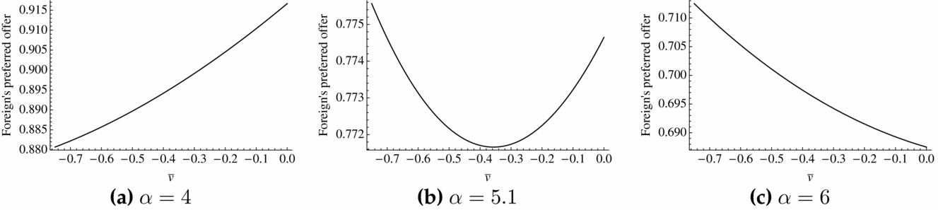




Comments
No Comments have been published for this article.