



%20--%3e%3c!DOCTYPE%20svg%20PUBLIC%20'-//W3C//DTD%20SVG%201.0//EN'%20'http://www.w3.org/TR/2001/REC-SVG-20010904/DTD/svg10.dtd'%3e%3csvg%20version='1.0'%20id='Layer_1'%20xmlns='http://www.w3.org/2000/svg'%20xmlns:xlink='http://www.w3.org/1999/xlink'%20x='0px'%20y='0px'%20width='64px'%20height='64px'%20viewBox='5.5%20-3.5%2064%2064'%20enable-background='new%205.5%20-3.5%2064%2064'%20xml:space='preserve'%3e%3cg%3e%3ccircle%20fill='%23FFFFFF'%20fill-opacity='0'%20cx='37.785'%20cy='28.501'%20r='28.836'/%3e%3cpath%20fill='%23595959'%20d='M37.441-3.5c8.951,0,16.572,3.125,22.857,9.372c3.008,3.009,5.295,6.448,6.857,10.314%20c1.561,3.867,2.344,7.971,2.344,12.314c0,4.381-0.773,8.486-2.314,12.313c-1.543,3.828-3.82,7.21-6.828,10.143%20c-3.123,3.085-6.666,5.448-10.629,7.086c-3.961,1.638-8.057,2.457-12.285,2.457s-8.276-0.808-12.143-2.429%20c-3.866-1.618-7.333-3.961-10.4-7.027c-3.067-3.066-5.4-6.524-7-10.372S5.5,32.767,5.5,28.5c0-4.229,0.809-8.295,2.428-12.2%20c1.619-3.905,3.972-7.4,7.057-10.486C21.08-0.394,28.565-3.5,37.441-3.5z%20M37.557,2.272c-7.314,0-13.467,2.553-18.458,7.657%20c-2.515,2.553-4.448,5.419-5.8,8.6c-1.354,3.181-2.029,6.505-2.029,9.972c0,3.429,0.675,6.734,2.029,9.913%20c1.353,3.183,3.285,6.021,5.8,8.516c2.514,2.496,5.351,4.399,8.515,5.715c3.161,1.314,6.476,1.971,9.943,1.971%20c3.428,0,6.75-0.665,9.973-1.999c3.219-1.335,6.121-3.257,8.713-5.771c4.99-4.876,7.484-10.99,7.484-18.344%20c0-3.543-0.648-6.895-1.943-10.057c-1.293-3.162-3.18-5.98-5.654-8.458C50.984,4.844,44.795,2.272,37.557,2.272z%20M37.156,23.187%20l-4.287,2.229c-0.458-0.951-1.019-1.619-1.685-2c-0.667-0.38-1.286-0.571-1.858-0.571c-2.856,0-4.286,1.885-4.286,5.657%20c0,1.714,0.362,3.084,1.085,4.113c0.724,1.029,1.791,1.544,3.201,1.544c1.867,0,3.181-0.915,3.944-2.743l3.942,2%20c-0.838,1.563-2,2.791-3.486,3.686c-1.484,0.896-3.123,1.343-4.914,1.343c-2.857,0-5.163-0.875-6.915-2.629%20c-1.752-1.752-2.628-4.19-2.628-7.313c0-3.048,0.886-5.466,2.657-7.257c1.771-1.79,4.009-2.686,6.715-2.686%20C32.604,18.558,35.441,20.101,37.156,23.187z%20M55.613,23.187l-4.229,2.229c-0.457-0.951-1.02-1.619-1.686-2%20c-0.668-0.38-1.307-0.571-1.914-0.571c-2.857,0-4.287,1.885-4.287,5.657c0,1.714,0.363,3.084,1.086,4.113%20c0.723,1.029,1.789,1.544,3.201,1.544c1.865,0,3.18-0.915,3.941-2.743l4,2c-0.875,1.563-2.057,2.791-3.541,3.686%20c-1.486,0.896-3.105,1.343-4.857,1.343c-2.896,0-5.209-0.875-6.941-2.629c-1.736-1.752-2.602-4.19-2.602-7.313%20c0-3.048,0.885-5.466,2.658-7.257c1.77-1.79,4.008-2.686,6.713-2.686C51.117,18.558,53.938,20.101,55.613,23.187z'/%3e%3c/g%3e%3c/svg%3e)
%20--%3e%3c!DOCTYPE%20svg%20PUBLIC%20'-//W3C//DTD%20SVG%201.0//EN'%20'http://www.w3.org/TR/2001/REC-SVG-20010904/DTD/svg10.dtd'%3e%3csvg%20version='1.0'%20id='Layer_1'%20xmlns='http://www.w3.org/2000/svg'%20xmlns:xlink='http://www.w3.org/1999/xlink'%20x='0px'%20y='0px'%20width='64px'%20height='64px'%20viewBox='5.5%20-3.5%2064%2064'%20enable-background='new%205.5%20-3.5%2064%2064'%20xml:space='preserve'%3e%3cg%3e%3ccircle%20fill='%23FFFFFF'%20fill-opacity='0'%20cx='37.637'%20cy='28.806'%20r='28.276'/%3e%3cg%3e%3cpath%20fill='%23595959'%20d='M37.443-3.5c8.988,0,16.57,3.085,22.742,9.257C66.393,11.967,69.5,19.548,69.5,28.5c0,8.991-3.049,16.476-9.145,22.456%20C53.879,57.319,46.242,60.5,37.443,60.5c-8.649,0-16.153-3.144-22.514-9.43C8.644,44.784,5.5,37.262,5.5,28.5%20c0-8.761,3.144-16.342,9.429-22.742C21.101-0.415,28.604-3.5,37.443-3.5z%20M37.557,2.272c-7.276,0-13.428,2.553-18.457,7.657%20c-5.22,5.334-7.829,11.525-7.829,18.572c0,7.086,2.59,13.22,7.77,18.398c5.181,5.182,11.352,7.771,18.514,7.771%20c7.123,0,13.334-2.607,18.629-7.828c5.029-4.838,7.543-10.952,7.543-18.343c0-7.276-2.553-13.465-7.656-18.571%20C50.967,4.824,44.795,2.272,37.557,2.272z%20M46.129,20.557v13.085h-3.656v15.542h-9.944V33.643h-3.656V20.557%20c0-0.572,0.2-1.057,0.599-1.457c0.401-0.399,0.887-0.6,1.457-0.6h13.144c0.533,0,1.01,0.2,1.428,0.6%20C45.918,19.5,46.129,19.986,46.129,20.557z%20M33.042,12.329c0-3.008,1.485-4.514,4.458-4.514s4.457,1.504,4.457,4.514%20c0,2.971-1.486,4.457-4.457,4.457S33.042,15.3,33.042,12.329z'/%3e%3c/g%3e%3c/g%3e%3c/svg%3e)
1. Introduction
The Taylor–Green vortex (TGV) (Taylor & Green Reference Taylor and Green1937) investigated in this study represents a simple yet well-defined flow configuration that exhibits rich physical phenomena, including the laminar-to-turbulent transition, posing a significant challenge for large-eddy simulation (LES) models. Understanding and accurately predicting this transition is crucial in numerous application areas such as wing aerodynamics and marine engineering. While most practical cases of laminar–turbulent transition involve boundary layers due to the presence of walls, the TGV provides a canonical benchmark for studying free transition in the absence of such effects. Owing to its well-known and straightforward set-up, the TGV has long served as a reference case for analysing the dynamics of turbulence (Orszag Reference Orszag, Glowinski and Lions1974; Brachet et al. Reference Brachet, Meiron, Orszag, Nickel, Morf and Frisch1983; Brachet Reference Brachet1991) and of vorticity fields (Sharma & Sengupta Reference Sharma and Sengupta2019).
With the growth of computational capabilities, unsteady flow simulations have become accessible to a wider scientific community. As a result, the TGV has gained popularity for the development and assessment of hybrid Reynolds-averaged Navier–Stokes (RANS)–LES approaches (Pereira et al. Reference Pereira, Grinstein, Israel, Rauenzahn and Girimaji2021), as well as pure LES methodologies (Domaradzki, Liu & Brachet Reference Domaradzki, Liu and Brachet1993; Ducros et al. Reference Ducros, Ferrand, Nicoud, Weber, Darracq, Gacherieu and Poinsot2006; Hickel, Adams & Domaradzki Reference Hickel, Adams and Domaradzki2006; Geier et al. Reference Geier, Lenz, Schönherr and Krafczyk2021; Jadhav & Chandy Reference Jadhav and Chandy2021; Engelmann et al. Reference Engelmann, Hasslberger, Baik, Klein and Kempf2023).
It has also proven valuable in code development and verification efforts (Orszag Reference Orszag, Glowinski and Lions1974; Fauconnier, De Langhe & Dick Reference Fauconnier, De Langhe and Dick2009; Ghosal & Lund Reference Ghosal and Lund2009; Tyliszczak Reference Tyliszczak2014; Bull & Jameson Reference Bull and Jameson2015), including applications in combustion modelling (Abdelsamie et al. Reference Abdelsamie, Lartigue, Frouzakis and Thévenin2021; Xu & Chen Reference Xu and Chen2023) and compressible flow simulations (Chapelier et al. Reference Chapelier2024). The initialisation of the TGV configuration is particularly straightforward: the initial velocity field is defined by a single wavelength that matches the size of the computational domain. As a result, filtering direct numerical simulation data to extract LES initial conditions becomes unnecessary. Additionally, due to its relatively short simulation times, high-resolution results can be achieved at modest computational cost. These advantages make the TGV an excellent test case for in-the-loop machine learning applications. For instance, it has been employed by Reissmann et al. (Reference Reissmann, Hasslberger, Sandberg and Klein2021) for gene expression programming (GEP)-based optimisation of LES models, as well as in the GEP-based derivation of LES models that incorporate correct asymptotic wall-scaling behaviour (Hasslberger et al. Reference Hasslberger, Reissmann, Sandberg and Klein2025). It is remarked that the tri-periodic, fully three-dimensional analytic solutions to the Navier–Stokes equations, as discussed in Antuono (Reference Antuono2020), are also closely related to the classical TGV problem. Beyond purely hydrodynamic turbulence, the TGV has further been extended to magnetohydrodynamic configurations and dynamo studies (i.e. the self-generation of magnetic field by a conducting moving fluid), where it provides a controlled setting for investigating linear and nonlinear dynamo mechanisms (Ponty et al. Reference Ponty, Mininni, Laval, Alexakis, Baerenzung, Daviaud, Dubrulle, Pinton, Politano and Pouquet2008).
Q-criterion iso-surfaces of the standard TGV (a) and the isotropic TGV (b) at a value of zero coloured using the normalised velocity magnitude
 $|U|/|U_{max}|$
at dimensionless times of
 $t/t_0 = 2.0$
,
 $t/t_0 = 10.0$
and
 $t/t_0 = 25.0$
from left to right.

Figure 1 illustrates the temporal evolution of the TGV. Initially, the flow is laminar, characterised by well-organised, large-scale vortex structures in which the kinetic energy is predominantly concentrated. As time advances, the flow experiences a nonlinear instability that initiates a cascade of energy from large to progressively smaller scales. This marks the onset of turbulence, during which the vortices interact, stretch and break down into finer-scale structures. At this stage, the flow is often assumed to closely resemble ideal homogeneous isotropic turbulence. Ultimately, in the absence of any external forcing, the turbulence decays due to viscous dissipation. Brachet et al. (Reference Brachet, Meiron, Orszag, Nickel, Morf and Frisch1983) demonstrated that the early evolution of the TGV retains its initial anisotropic character, but at higher Reynolds numbers, the flow becomes nearly isotropic for high wavenumbers. This has also been confirmed by Hickel et al. (Reference Hickel, Adams and Domaradzki2006), who note that statistical isotropy at small scales can be reasonably achieved in the decaying stages of the TGV. More recently, high-resolution simulations of the TGV have been employed to study spectral energy transfer, bottleneck effects and thermalised ranges in turbulent cascades, including investigations based on hyperviscous formulations (Agrawal et al. Reference Agrawal, Alexakis, Brachet and Tuckerman2020), essentially a method to mimic flows with extremely large Reynolds numbers.
It is worth noting that the assumptions of isotropy and homogeneity in homogeneous isotropic turbulence impose very strong requirements, far more restrictive than the conditions typically considered in RANS second-order closure modelling, as they demand directional and spatial invariance of all statistical properties, including higher-order moments or two-point statistics. In addition to these mathematical properties, isotropic turbulence is characterised by several well-known physical features. In fact, a recent study by Engelmann et al. (Reference Engelmann, Hasslberger, Baik, Klein and Kempf2023) revealed considerable and persistent anisotropy for plane-averaged velocity statistics of the TGV, presumably imprinted by the initial conditions and the tri-periodic, finite-size computational domain. To the best of the authors’ knowledge, the homogeneity and isotropy of the TGV (in the above sense) have not been studied in detail in the available literature, particularly not for different initial conditions.
Following Kolmogorov’s seminal perspective on turbulence (Kolmogorov Reference Kolmogorov1941a , Reference Kolmogorovb ), the energy cascade along the spectrum of turbulent kinetic energy is accompanied by a progressive loss of information. While the large-scale motions are strongly influenced by the geometry of the flow, it is hypothesised that the small scales, at sufficiently high Reynolds numbers, exhibit universal behaviour and are therefore more amenable to modelling. This assumption forms a cornerstone of both turbulence theory and LES approaches. From a theoretical perspective, spontaneous isotropisation in decaying turbulence is expected to occur primarily at sufficiently small scales, where nonlinear interactions dominate and universality emerges, as emphasised by Kolmogorov and discussed in detail by Frisch (Reference Frisch1995). In contrast, large-scale motions are not necessarily expected to homogenise or isotropise fully, particularly in flows such as the TGV, where persistent symmetries and impermeable subdomains, imprinted by the symmetry-preserving nature of the Navier–Stokes equations (Bardos et al. Reference Bardos, Lopes Filho, Niu, Nussenzveig Lopes and Titi2013; Barker, Prange & Tan Reference Barker, Prange and Tan2024), constrain the dynamics. Nevertheless, the TGV is often interpreted as approaching a homogeneous or homogeneous–isotropic state at late times, at least in an approximate sense, as assumed in several previous studies (Kulikov & Son Reference Kulikov and Son2018; Nathen et al. Reference Nathen, Haussmann, Krause and Adams2018; Hartmann Reference Hartmann, Hirsch, Hillewaert, Hartmann, Couaillier, Boussuge, Chalot, Bosniakov and Haase2021). Accordingly, it is of fundamental importance to examine whether the TGV satisfies the key criteria of homogeneity and isotropy, as this constitutes the basis for its suitability as a model problem for studying turbulent flows and developing turbulence models. Understanding the extent to which isotropisation and homogenisation may emerge from non-homogeneous and non-isotropic periodic initial conditions remains a fundamental problem in turbulence research. Addressing this issue in a general sense is beyond the scope of the present study. Instead, we apply a suite of isotropy and homogeneity tests to assess and quantify the evolution of these properties in time. This also includes different initial conditions, such as the isotropised TGV variant of Ono et al. (Reference Ono, Chitose, Suzuki and Kouchi2024).
2. Problem description
We consider an incompressible flow described by the Navier–Stokes equations defined as
 \begin{align} \frac {\partial {u_{{\!j}}}} {\partial x_{{\!j}}} &= 0, \nonumber\\ \frac {\partial \rho {u_i}}{\partial t} + \frac {\partial \rho {u_{{i}}} {u_{{\!j}}}}{\partial x_{{\!j}}} &= \frac {\partial }{\partial x_{{\!j}}} \left ( \mu \left ( \frac {\partial {u_{{i}}}}{\partial x_{{\!j}}} + \frac {\partial {u_{{\!j}}}}{\partial x_{{i}}} \right )\right ) -\frac {\partial {p}}{\partial x_{{i}}}, \end{align}
where
 $u_i$
stands for the velocity components (
 $u,\,v,\,w$
),
 $p$
the pressure,
 $\rho$
the mass density and
 $\mu$
the dynamic viscosity. The TGV domain features a length of
 $2\pi l_0$
(
 $l_0$
is the reference length) in each dimension. The assumed periodicity eliminates the need to impose numerical boundary conditions, a common Achilles’ heel of numerical simulations. At the same time, it allows the application of specialised high-order numerical codes, as discussed in § 4.
Two TGV configurations are considered, labelled as standard and referred to in the introduction, and isotropic, which will be introduced shortly. The initial velocity field for the standard TGV is given by the following expressions:
 \begin{align} u\left (x,y,z,t=0\right ) &= U_0\cos \left (x\right )\sin \left (y\right )\sin \left (z\right )\!,\nonumber\\ v\left (x,y,z,t=0\right ) &= -U_0\sin \left (x\right )\cos \left (y\right )\sin \left (z\right )\!,\nonumber\\ w\left (x,y,z,t=0\right ) &=0, \end{align}
where
 $U_0$
is the reference velocity. The initial pressure field is obtained from the Poisson equation:
 \begin{equation} {\nabla} ^2 p = -\rho \, \boldsymbol{\nabla }\boldsymbol{\cdot }\left [ (\boldsymbol{u} \boldsymbol{\cdot }\boldsymbol{\nabla })\boldsymbol{u} \right ], \end{equation}
formulated by noting that the viscous term is zero for incompressible flows (
 $\boldsymbol{\nabla }\boldsymbol{\cdot }({\nabla} ^2 \boldsymbol{u})={\nabla} ^2 (\boldsymbol{\nabla }\boldsymbol{\cdot }\boldsymbol{u})=0$
). It is defined as
 \begin{equation} p\left (x,y,z,t=0\right ) = \frac {\rho U_0^2}{16} \left ( \cos (2x) + \cos (2y) \right ) \left ( \cos (2z) - 2 \right ). \end{equation}
The initial velocity field (2.2) fits under an umbrella of general initial conditions defined by Taylor & Green (Reference Taylor and Green1937) in the form
 \begin{align} u\left (x,y,z,t=0\right ) &= A \cos \left (a x\right )\sin \left (b y\right )\sin \left (c z\right )\!,\nonumber\\ v\left (x,y,z,t=0\right ) &= B \sin \left (a x\right )\cos \left (b y\right )\sin \left (c z\right )\!,\nonumber\\ w\left (x,y,z,t=0\right ) &= C \sin \left (a x\right )\sin \left (b y\right )\cos \left (c z\right )\!, \end{align}
where the condition
 $Aa+Bb+Cc=0$
ensures continuity. As the wavenumbers
 $a,b,c$
are positive quantities, the velocity field (2.5) cannot be made isotropic. Using a modified initial condition, Ono et al. (Reference Ono, Chitose, Suzuki and Kouchi2024) introduced the isotropic TGV. Its initialisation, scaled to obtain the same kinetic energy as for the standard TGV, reads
 \begin{align} u(x,y,z,t=0) &= U_0 /\sqrt {6}\left ( -\cos (x)\sin (y) + \cos (x)\sin (z) \right )\!, \nonumber \\ v(x,y,z,t=0) &= U_0 /\sqrt {6}\left ( -\cos (y)\sin (z) + \cos (y)\sin (x) \right )\!, \nonumber \\ w(x,y,z,t=0) &= U_0 /\sqrt {6}\left ( -\cos (z)\sin (x) + \cos (z)\sin (y) \right )\!, \nonumber \\ p\left (x,y,z,t=0\right ) &= \frac {\rho U_0^2}{6} \left [ \!\left ( \!\frac {1}{6} \cos (2x) - \frac {1}{2} \!\right ) \sin (y) \sin (z) + \left ( \!\frac {1}{6} \cos (2y) - \frac {1}{2} \!\right ) \sin (x) \sin (z) \right .\nonumber \\ & \left .+ \left ( \!\frac {1}{6} \cos (2z) - \frac {1}{2}\! \right ) \sin (x) \sin (y) - \frac {1}{2} \left ( \cos (2x) + \cos (2y) + \cos (2z) \right )\! \right ]\!. \end{align}
In both cases, the reference velocity and length are taken as
 $U_0 = 1\ \rm {m\,s^{-1}}$
and
 $l_0 = 1\ \textrm {m}$
. The time scales are
 $t_0 = 1\ \textrm {s}$
for the standard TGV and
 $t_0 = 2\ \textrm {s}$
for the isotropic TGV. In the latter case, the flow field develops more slowly, and adopting the longer reference time scale allows the results to be presented within the same plots. A Reynolds number of
 $Re=\rho U_0 l_0 / \mu =1600$
at initialisation is achieved by setting the density to
 $\rho =1\ \rm {kg\,m}^{-3}$
and the dynamic viscosity to
 $\mu =0.625\boldsymbol{\times }10^{-3}\ \textrm {Pa s}$
. We note that this particular value of the Reynolds number was selected following Brachet et al. (Reference Brachet, Meiron, Orszag, Nickel, Morf and Frisch1983), and it has also been used in several subsequent studies (Hickel et al. Reference Hickel, Adams and Domaradzki2006; Van Rees et al. Reference Van Rees, Leonard, Pullin and Koumoutsakos2011; Jadhav & Chandy Reference Jadhav and Chandy2021).
3. Theoretical background
The TGV is analysed using quantities that characterise the effects of turbulence, such as Reynolds stresses
 $R_{ij}=\langle u_i u_{\!j} \rangle -\langle u_i \rangle \langle u_{\!j} \rangle$
, turbulent kinetic energy
 $k=R_ {ii}/2$
and coherent structure function
 $F_{{\textit{CS}}}$
(Kobayashi Reference Kobayashi2005). Here, the angled brackets denote a suitable averaging operation. In the context of this work, averaging is performed either globally in space or along
 $x{-}y$
planes and lines at a fixed instant in time. In the latter case, the resulting profiles are plotted as a function of the plane-normal direction
 $z$
. The coherent structure function is defined as
 \begin{equation} F_{ {\textit{CS}}} = \frac {Q}{E}, \end{equation}
which is the ratio of the second invariant of the velocity gradient tensor:
 \begin{equation} Q = -\frac {1}{2}\frac {\partial {u}_{\!j}}{\partial x_{i}}\frac {\partial {u}_{i}}{\partial {x}_{\!j}} = \frac {{\nabla} ^2 p}{2\rho } \end{equation}
and its respective magnitude squared:
 \begin{equation} E = \frac {1}{2}\frac {\partial {u}_{\!j}}{\partial x_{i}}\frac {\partial {u}_{\!j}}{\partial x_{i}}. \end{equation}
The coherent structure function is an instructive quantity, as it captures the relationship between dissipation and enstrophy, two fundamental measures used to characterise the structure of turbulent flows. Being a strictly bounded quantity (
 $-1 \lt F_{ {\textit{CS}}} \lt +1$
), it exhibits mathematical elegance, and the iso-contour
 $F_{{\textit{CS}}} = 0$
identifies the state of dissipation–enstrophy equilibrium. Moreover,
 $F_{{\textit{CS}}}$
can be interpreted as a suitably normalised form of the
 $Q$
-criterion, which is commonly employed in the literature to detect enstrophy-dominated regions in turbulent flows.
The anisotropy in a turbulent flow can be conveniently characterised with the help of the Lumley triangle (Lumley Reference Lumley1979). Its boundaries are given as a function of the second and third invariant of the anisotropy tensor
 $ a_{ij} = R_{ij}/ R_{kk}-\delta _{ij}/3$
:
 \begin{equation} \textrm {II}\left (a\right ) = \left (\textrm {trace}\left (a\right )^2-\textrm {trace}\left (a^2\right )\right )/2, \ \ \ \ \ \ \textrm {III}\left (a\right ) = \left (\textrm {det}\left (a\right )\right ) \end{equation}
and by introducing the variables
 \begin{equation} \eta = \left (-\textrm {II}\left (a\right )/3\right )^{1/2} , \ \ \ \ \ \ \xi = \left (-\textrm {III}\left (a\right )/2\right )^{1/3}. \end{equation}
Any physically realisable state of the anisotropy tensor
 $a_{ij}$
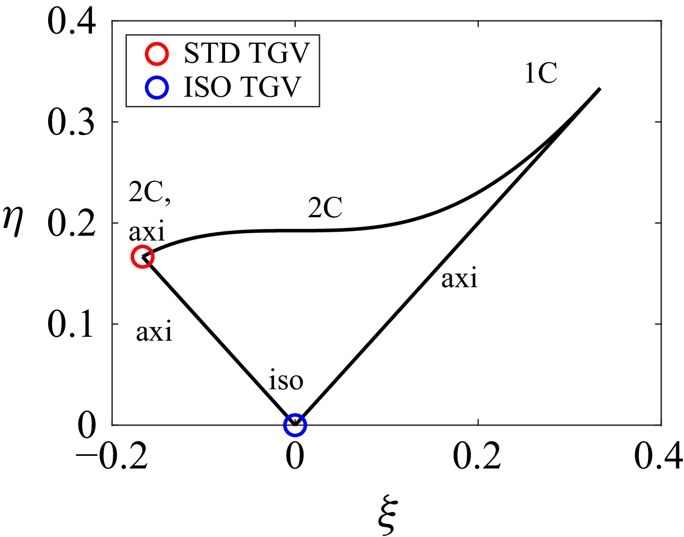
lies within the triangle shown exemplarily in figure 2 for the standard and isotropic TGVs at initialisation, i.e.
 $t/t_0=0$
. The left and right borders of the triangle represent an axisymmetric contraction and expansion, respectively, while the upper border denotes the two-component state. Finally, the isotropic state corresponds to the lower corner
 $ (\xi ,\eta )= (0,0 )$
. By analogy, the anisotropy of the dissipation tensor
 \begin{equation} \varepsilon _{ij} =2\nu \left \langle \frac {\partial u_i^{\prime}}{\partial x_k}\frac {\partial u_{\!j}^{\prime}}{\partial x_k} \right \rangle =2\nu \left ( \left \langle \frac {\partial u_i}{\partial x_k}\frac {\partial u_{\!j}}{\partial x_k} \right \rangle -\left \langle \frac {\partial u_i}{\partial x_k} \right \rangle \left \langle \frac {\partial u_{\!j}}{\partial x_k} \right \rangle \right ) \end{equation}
can be defined, where
 $u_i^{\prime}=u_i-\langle u_i\rangle$
. Since dissipation predominantly occurs at small flow scales, it provides insight into the small-scale anisotropy of the flow.
Anisotropy of the Reynolds stresses in the Lumley triangle, exemplarily shown for the standard (STD) TGV and isotropic (ISO) TGV flow at
 $t/t_0=0$
. The following abbreviations are used: 1C, one-component; 2C, two-component; axi, axisymmetric; iso, isotropic.

The homogeneity of the TGV is analysed by a homogeneity measure introduced by Germano and co-workers (Errante et al. Reference Errante, Klein, Ferrero, Larocca, Scovazzi and Germano2024). It is based on considering a mixed averaging procedure, where
 $\langle \boldsymbol{\cdot }\rangle _\alpha$
denotes averaging in (homogeneous) direction
 $x_\alpha$
,
 $\langle \boldsymbol{\cdot }\rangle _{\alpha \beta }$
denotes averaging in both (homogeneous) directions
 $x_\alpha ,x_\beta$
and
 $\langle \boldsymbol{\cdot }\rangle _{\alpha \beta \gamma }$
denotes averaging in volume. In the general case, time averaging can be included as well, but this does not apply for the TGV, because of its unsteady nature. The choice of the averaging procedure gives rise to a corresponding generalised central moment (Germano Reference Germano1992), signifying the Reynolds stresses determined from averaging in the given direction(s) (when applied to the velocity components):
 \begin{equation} \tau _{\alpha }(u_i,u_{\!j})=\langle u_i u_{\!j} \rangle _{\alpha } -\langle u_i \rangle _{\alpha } \langle u_{\!j} \rangle _{\alpha }, \ \ \ \tau _{\alpha \beta }(u_i,u_{\!j})=\langle u_i u_{\!j} \rangle _{\alpha \beta } -\langle u_i \rangle _{\alpha \beta } \langle u_{\!j} \rangle _{\alpha \beta }, \ \ \ldots \end{equation}
Averaging
 $\tau _\alpha$
in the
 $\beta$
direction and making use of
 $\langle \langle \boldsymbol{\cdot }\rangle _\alpha \rangle _\beta = \langle \langle \boldsymbol{\cdot }\rangle _\beta \rangle _\alpha = \langle \boldsymbol{\cdot }\rangle _{\alpha \beta }$
results in
 \begin{equation} \langle \tau _{\alpha }(u_i,u_{\!j})\rangle _\beta =\langle u_i u_{\!j} \rangle _{\alpha \beta } -\langle \langle u_i \rangle _{\alpha } \langle u_{\!j} \rangle _{\alpha } \rangle _\beta . \end{equation}
Inserting (3.8) into (3.7) for
 $\tau _{\alpha \beta }$
and using
 $\tau _{\beta }(\langle u_i \rangle _\alpha ,\langle u_{\!j} \rangle _\alpha )= \langle \langle u_i \rangle _\alpha \langle u_{\!j} \rangle _\alpha \rangle _{\beta } -\langle \langle u_i \rangle _\alpha \rangle _{\beta } \langle \langle u_{\!j} \rangle _\alpha \rangle _{\beta }$
finally gives rise to
 \begin{eqnarray} \tau _{\beta \alpha }(u_i,u_{\!j})&=& \langle \tau _{\alpha }(u_i,u_{\!j})\rangle _\beta + \tau _{\beta }(\langle u_i \rangle _\alpha ,\langle u_{\!j} \rangle _\alpha ) \nonumber \\ &=& \langle \tau _{\beta }(u_i,u_{\!j})\rangle _\alpha + \tau _{\alpha }(\langle u_i \rangle _\beta ,\langle u_{\!j} \rangle _\beta )= \tau _{\alpha \beta }(u_i,u_{\!j}) \end{eqnarray}
for a two-dimensional partition and
 \begin{eqnarray} \tau _{\gamma \beta \alpha }(u_i,u_{\!j})&=& \langle \tau _{\alpha }(u_i,u_{\!j})\rangle _{\beta \gamma }+ \tau _{\beta \gamma }(\langle u_i\rangle _\alpha ,\langle u_{\!j}\rangle _\alpha ) = \cdots \nonumber \\ &=&\langle \tau _{\alpha \beta }(u_i,u_{\!j})\rangle _{\gamma }+ \tau _{\gamma }(\langle u_i\rangle _{\alpha \beta },\langle u_{\!j}\rangle _{\alpha \beta }) = \cdots \end{eqnarray}
for a three-dimensional partition of the statistical measure. Based on this, we define the following measures of homogeneity in two-dimensional partitions:
 \begin{equation} M_{\alpha (\beta )}(u_i,u_{\!j})= \frac {\langle \tau _{\alpha }(u_i,u_{\!j})\rangle _{\beta }} {\tau _{ \beta \alpha }(u_i,u_{\!j})} = 1-\frac {\tau _{\beta }(\langle u_i\rangle _\alpha ,\langle u_{\!j}\rangle _\alpha )} {\tau _{\beta \alpha }(u_i,u_{\!j})} \end{equation}
and the following in three-dimensional partitions:
 \begin{align}& M_{\alpha (\beta \gamma )}(u_i,u_{\!j})= \frac {\langle \tau _{\alpha }(u_i,u_{\!j})\rangle _{\beta \gamma }} {\tau _{\gamma \beta \alpha }(u_i,u_{\!j})} = 1-\frac {\tau _{\beta \gamma }(\langle u_i\rangle _\alpha ,\langle u_{\!j}\rangle _\alpha )} {\tau _{\gamma \beta \alpha }(u_i,u_{\!j})}, \end{align}
 \begin{align}& M_{\alpha \beta (\gamma )}(u_i,u_{\!j})= \frac {\langle \tau _{\alpha \beta }(u_i,u_{\!j})\rangle _{\gamma }} {\tau _{\gamma \beta \alpha }(u_i,u_{\!j})} = 1-\frac {\tau _{\gamma }(\langle u_i\rangle _{\alpha \beta },\langle u_{\!j}\rangle _{\alpha \beta })} {\tau _{\gamma \beta \alpha }(u_i,u_{\!j})}. \end{align}
These indices allow for quantification of the relative contribution by averaging in different directions to the evaluation of the statistics. For example, an index of
 $M_{\alpha (\beta \gamma )}\approx 1$
indicates that Reynolds stresses are equally well captured for
 $\tau _{\alpha \beta \gamma }$
and
 $\tau _{\alpha }$
statistics. From a probabilistic point of view this implies that there is a sufficient number of statistically independent samples in the
 $x_\alpha$
direction. If the diagonal components of the Reynolds stresses are considered, i.e.
 $i=j$
, we write in the following more briefly
 $M_{\alpha \beta (\gamma )}(u_i)$
instead of
 $M_{\alpha \beta (\gamma )}(u_i,u_i)$
. For an isotropic flow, the quantity
 $M_{\alpha (\beta \gamma )}(u_i)$
should, in a statistical sense, be the same under rotation of the coordinate system, i.e.
 \begin{align} M_{x(yz)}(u)&=M_{y(xz)}(v)=M_{z(xy)}(w), \nonumber \\ M_{y(xz)}(u)&=M_{z(xy)}(u)=M_{x(yz)}(v)=M_{z(xy)}(v)= M_{x(yz)}(w)=M_{y(xz)}(w). \end{align}
We can define indices of homogeneity also for other quantities, in particular for the pressure
 $p$
. We can write
 \begin{equation} M_{\alpha (\beta \gamma )}(p)= \frac {\langle \tau _{\alpha }(p,p)\rangle _{\beta \gamma }} {\tau _{\gamma \beta \alpha }(p,p)}= 1-\frac {\tau _{\beta \gamma }(\langle p\rangle _\alpha ,\langle p\rangle _\alpha )} {\tau _{\gamma \beta \alpha }(p,p)} \end{equation}
and
 \begin{equation} M_{\alpha \beta (\gamma )}(p)= \frac {\langle \tau _{\alpha \beta }(p,p)\rangle _{\gamma }} {\tau _{\gamma \beta \alpha }(p,p)}= 1-\frac {\tau _{\gamma }(\langle p\rangle _{\alpha \beta },\langle p\rangle _{\alpha \beta })} {\tau _{\gamma \beta \alpha }(p,p)} \end{equation}
that we apply in the following to study the homogeneity of the pressure statistics in TGV flow, an argument that we think is largely unexplored.
In turbulent flows, the number of statistically independent spatial samples is inversely proportional to the integral length scale, which is obtained by integrating the appropriate normalised two-point correlation function
 \begin{equation} \chi _{\phi ,\psi ,i}(\boldsymbol{x} ,r)=\langle \phi (\boldsymbol{x}),\psi (\boldsymbol{x}+\boldsymbol{e_i} r) \rangle \big / \langle \phi (\boldsymbol{x}),\psi (\boldsymbol{x}) \rangle \end{equation}
from
 $r=0 \ldots r_+$
, where
 $r_+$
denotes the first root such that
 $\chi _{\phi ,\psi ,i}(\boldsymbol{x}, r_+)=0$
(i.e. the positive lobe convention is applied). For the TGV, the averaging operator
 $\langle \boldsymbol{\cdot }\rangle$
is taken over all three spatial directions, allowing the dependence on
 $\boldsymbol{x}$
to be omitted. The integral length scale is defined as
 \begin{equation} L_{\phi \psi ,i}=\int _0^{r_+} \chi _{\phi ,\psi ,i}(r)\, {\rm d}r. \end{equation}
In the case of the velocity field, the longitudinal integral length scales are denoted compactly as
 $L_{ii,i}$
(in place of
 $L_{u_iu_i,i}$
) and, analogously, the transverse length scales as
 $L_{ii,j}$
for
 $i\ne j$
. Knowing that for homogeneous, isotropic turbulence, the longitudinal and transverse length scales are related by Pope (Reference Pope2000)
 \begin{equation} L_{ii,i}=2 L_{ii,j\ne i} \end{equation}
we examine whether or to what extent the above relation holds for the TGV evolution.
4. Numerical methods
The simulations are carried out using the academic high-order code SAILOR, which employs a projection method to couple pressure and velocity fields. Time integration is performed using a second-order Adams–Bashforth/Adams–Moulton predictor–corrector scheme, while spatial discretisation relies on a tenth-order compact finite-difference method. The numerical formulation uses half-staggered meshes (Tyliszczak Reference Tyliszczak2014, Reference Tyliszczak2016), where velocity components share the same grid points, and pressure nodes are shifted by half a grid spacing. This arrangement simplifies the code implementation and improves computational efficiency, as only limited interpolation between nodes is required. The half-staggering of pressure nodes provides sufficiently strong velocity–pressure coupling, effectively preventing the spurious pressure oscillations typical of collocated grids. Further details on derivative approximations and the interpolation procedure between velocity and pressure nodes can be found in Tyliszczak (Reference Tyliszczak2014, Reference Tyliszczak2016). The SAILOR code has been extensively validated in fully periodic two- and three-dimensional configurations (Tyliszczak Reference Tyliszczak2014; Caban & Tyliszczak Reference Caban and Tyliszczak2022; Caban et al. Reference Caban, Tyliszczak, Geurts and Domaradzki2025), as well as in free-flow cases involving mixed boundary conditions and varying levels of physical complexity (see Tyliszczak Reference Tyliszczak2018; Boguslawski, Wawrzak & Tyliszczak Reference Boguslawski, Wawrzak and Tyliszczak2019; Li et al. Reference Li, Noack, Wang, Cornejo, Guy, Pickering, Shaqarin and Tyliszczak2024; Wawrzak et al. Reference Wawrzak, Boguslawski and Tyliszczak2024a , Reference Wawrzak, Stempka and Tyliszczakb and references therein). Across all these studies, the code consistently demonstrated high computational efficiency and accuracy. Given that the present simulations concern a geometrically simple configuration with three-dimensional periodicity, similar performance can be expected in the current work.
The computations are carried out on a uniform mesh with
 $N=256$
nodes in each spatial direction. The time step is set to
 $\Delta t=10^{-3}$
s (
 $\text{CFL}=\Delta t U_0/h\approx 0.04$
, where
 $h=2\pi l_0/N$
is the grid spacing), and the simulations are run up to
 $t=100\,t_0$
. The maximum ratio of the Kolmogorov length scale to the grid spacing is
 $\eta _K/h=0.49$
and
 $\eta _K/h=0.67$
for the standard and isotropic TGV initialisations, respectively. Hence, the mesh fulfils the criterion for good resolution of the smallest scales (Pope Reference Pope2000). Indeed the results show very good agreement with the spectral code reference data by Brachet et al. (Reference Brachet, Meiron, Orszag, Nickel, Morf and Frisch1983) and Hillewaert (Reference Hillewaert2011). Detailed comparisons are provided in the supplementary material available at [https://doi.org/10.1017/jfm.2026.11380], including the temporal evolution of kinetic energy and its dissipation, amplitude spectra, selected homogeneity indices and a mesh sensitivity analysis using meshes with
 $N=384$
and
 $N=512$
nodes in each spatial direction. In all cases, the results show excellent agreement with one another and with the reference data, with only very minor quantitative differences that do not affect the qualitative conclusions of this work.
(a) Turbulent kinetic energy (TKE) and its dissipation. (b) Turbulent integral length scales and Kolmogorov scale. (c) Coherent structure function. All results are shown for the standard (STD) TGV and isotropic (ISO) TGV. The time scale
 $t_0$
for the isotropic TGV is twice that of the standard TGV.

5. Results
The discussion of the results is divided into two subsections. First, global statistics are presented to evaluate the isotropy of the TGV. Subsequently, the homogeneity of the TGV is examined based on
 $x,y$
-plane averages. Additionally, for the pressure field the homogeneity indices based on line and plane statistics are compared.
5.1. Global statistics
Both TGV cases start from the same initial turbulent kinetic energy (
 $k=U_0^2/8$
), as shown in figure 3(a). Although the simulation time for the isotropic TGV is twice that of the standard case, the evolution of kinetic energy becomes similar when normalised by the time scale
 $t_0$
. The isotropic TGV exhibits a markedly lower peak of the dissipation rate (
 $\epsilon =-{\rm d}k/{\rm d}t$
), characterised by an extended plateau with two local maxima.
Because of the smaller dissipation rate, the Kolmogorov scale
 $\eta _K$
is larger for the isotropic TGV around the time of
 $\epsilon$
peak (figure 3
b). The size of the energy carrying structures can be estimated as
 $\sim k^{3/2}/\epsilon$
. Hence the considerably smaller dissipation rate is reflected in larger turbulent structures and this can be seen from the mean value of the three longitudinal integral length scales as well. While figure 3 shows the average of
 $L_{ii}$
, it is noted (see figure 9) that for the isotropic TGV we have
 $L_{11}=L_{22}=L_{33}$
while for the standard TGV
 $L_{11}=L_{22}\gt L_{33}$
throughout the simulation.
The coherent structure function in figure 3(c) depicts positive values (i.e. dominance of rotation rate) for small values of
 $t/t_0$
(except for
 $t=0$
where the standard TGV starts from strain–rotation equilibrium, i.e.
 $F_{\textit{CS}}=0$
), while towards the end of the simulation it tends towards small negative values approaching
 $-0.1$
as expected for isotropic turbulence (Kobayashi Reference Kobayashi2005).
Figure 4 shows the globally averaged Reynolds stress anisotropy in the Lumley triangle for both TGVs over time. The standard TGV starts from the two-component axisymmetric corner (note that
 $w=0$
for
 $t=0$
) and evolves along the axisymmetric contraction border (i.e.
 $R_{11}=R_{22}\gt R_{33}$
) towards the isotropic state without fully reaching it. Around
 $t/t_0=8$
it reverses directions and slowly departs again from the isotropic state towards
 $(\xi ,\eta )=(-0.057,0.057)$
for
 $t/t_0=25$
. This departure from isotropy can also be seen from the Reynolds stresses shown in figure 7, where around
 $t/t_0=8$
the Reynolds stresses are closest to each other. Subsequently, the flow loses energy rapidly and the isotropy state remains close to its position for
 $t/t_0=25$
, even up to
 $t/t_0=100$
(not shown in the figure), where it attains the values
 $(\xi ,\eta )=(-0.073,0.073)$
.
The isotropic TGV, on the other hand, starts from a perfectly isotropic state and remains there throughout the simulation. This behaviour is consistent with the diagonal components of the Reynolds stresses shown later in figures 7 and 8. Dissipation occurs predominantly at small scales and the Lumley triangle for the dissipation tensor is shown in figure 5. Although the behaviour is qualitatively similar to the isotropy of the Reynolds stress tensor, it is noted that for
 $t/t_0\gt 10$
the dissipation tensor for the standard TGV has become more isotropic. This is consistent with earlier observations from the literature that the flow becomes nearly isotropic for large wavenumbers (Brachet et al. Reference Brachet, Meiron, Orszag, Nickel, Morf and Frisch1983; Hickel et al. Reference Hickel, Adams and Domaradzki2006) and with simulations in different flow configurations (Klein et al. Reference Klein, Trummler and Radtke2022a
,
Reference Klein, Trummler, Urban and Chakrabortyb
), indicating a higher isotropy for the dissipation tensor compared with the Reynolds stress tensor.
Turbulence state based on Reynolds stresses plotted in the Lumley triangle over time. (a) Standard TGV. (b) Isotropic TGV. The time scale
 $t_0$
for the isotropic TGV is twice that of the standard TGV.

Turbulence state based on the dissipation tensor plotted in the Lumley triangle over time. (a) Standard TGV. (b) Isotropic TGV. The time scale
 $t_0$
for the isotropic TGV is twice that of the standard TGV.

Pressure variance (a) and pressure-based length scales
 $L_{pp,i}, \ i=1,2,3$
(b). Homogeneity indices
 $M_{\alpha (\beta \gamma )}(p)$
(c) and homogeneity indices
 $M_{\alpha \beta (\gamma )}(p)$
(d) for the standard (STD) TGV and isotropic (ISO) TGV.

The homogeneity indices are discussed next. Starting with the pressure as a scalar quantity, figure 6(c) shows
 $M_{\alpha (\beta \gamma )}(p)$
and figure 6(d) shows
 $M_{\alpha \beta (\gamma )}(p)$
, i.e. the homogeneity indices comparing the pressure variance based on line statistics (3.15) and plane statistics (3.16) against the pressure variance based on three-dimensional averages. For the isotropic TGV the homogeneity indices are identical under permutation of the indices
 $\alpha , \beta , \gamma$
, while for the standard TGV we have
 $M_{1(23)}(p)=M_{2(13)}(p)\gt M_{3(12)}(p)$
for
 $0\le t/ t_0\le 4$
and
 $t/t_0\gt 12$
. This suggests less independent samples in the
 $z$
direction or equivalently larger integral scales of the pressure field in this direction, i.e.
 $L_{pp,3}^{\textit{STD}}\gt L_{pp,1}^{\textit{STD}}=L_{pp,2}^{\textit{STD}}$
, which is indeed the case for these points in time as can be seen in figure 6(b). For the same reason we have
 $M_{12(3)}(p)\gt M_{23(1)}(p)=M_{13(2)}(p)$
for
 $0\le t/t_0\le 4$
and
 $t/t_0\gt 12$
, since
 $y{-}z$
- or
 $x{-}z$
-plane statistics of pressure variance contain a smaller number of statistically independent samples compared with
 $x{-}y$
-plane statistics. This behaviour clearly shows the close relation of the homogeneity indices with the integral scales of turbulence. However, while the two-point autocorrelation function
 $\chi$
can be easily computed from its definition, such a naive approximation tends to be noisy with over- and undershoots and oscillations, which can lead to poor estimates of integral length scales (Oliver et al. Reference Oliver, Malaya, Ulerich and Moser2014). Conversely, the homogeneity indices do not suffer from this problem. The following discussion is limited to the homogeneity indices based on line statistics such as
 $M_{\alpha (\beta \gamma )}(\boldsymbol{\cdot })$
which are easier to analyse.
Results for the standard TGV. (a) Reynolds stress components
 $R_{ii},\ i=1,2,3$
. (b–d) Homogeneity indices
 $M_{\alpha (\beta \gamma )}(u_i),\ i=1,2,3$
.

Results for the isotropic TGV. (a) Reynolds stress components
 $R_{ii},\ i=1,2,3$
. (b–d) Homogeneity indices
 $M_{\alpha (\beta \gamma )}(u_i),\ i=1,2,3$
.

We consider the different velocity components next. The homogeneity indices of the individual velocity components
 $M_{\alpha (\beta \gamma )}(u_i)$
are shown in figures 7 and 8 for the standard and isotropic TGVs together with the Reynolds stresses plotted over time. The homogeneity indices
 $M_{\alpha (\beta \gamma )}(u)$
and
 $M_{\alpha (\beta \gamma )}(v)$
start from unity for the standard TGV and decrease slightly during the course of the simulation. For
 $M_{\alpha (\beta \gamma )}(w)$
the behaviour is different for small times but it is noted that
 $w=0$
for
 $t=0$
, which makes the computation of
 $M_{\alpha (\beta \gamma )}(w)$
ill-conditioned for small times. In all cases it is observed that
 $M_{i(jk)}(u_i)\gt M_{j(ik)}(u_i)$
and
 $M_{i(jk)}(u_i)\gt M_{k(ij)}(u_i)$
. A different behaviour is observed for the isotropic TGV where at
 $t=0$
 $M_{i(j,k)}(u_i)=1$
, while
 $M_{j(i,k)}(u_i)=0.5$
and
 $M_{k(i,j)}(u_i)=0.5$
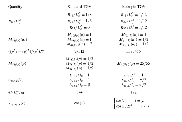
. This can be also shown by analytical integration of the initial conditions and a compilation of selected analytical results for
 $t=0$
is shown in table 2. Nevertheless, also for the isotropic TGV we have
 $M_{i(jk)}(u_i)\gt M_{j(ik)}(u_i)$
. This can be explained from the behaviour of the longitudinal and transverse length scales shown in figure 9. For both TGVs it is immediately clear that larger integral scales (in either longitudinal or transverse direction) are related to smaller homogeneity indices; compare the markers in figures 7 and 8 with those in figure 9. As an example, the largest integral scale for the
 $u$
velocity component of the standard TGV corresponds to
 $L_{11,2}$
. This yields the smallest number of statistically independent samples for line statistics of
 $R_{11}$
in the
 $y$
direction and consequently
 $M_{2(13)}(u)$
is the smallest among the
 $u$
homogeneity indices. As an alternative example we have for the isotropic TGV
 $L_{11,2}\approx L_{11,3} \gt L_{11,1}$
(i.e. far from relation (3.19)) and hence
 $M_{1(23)}(u)\gt M_{2(13)}(u) \approx M_{3(12)}(u)$
. Similar considerations apply for the
 $v$
and
 $w$
velocity components.
Apart from these quantitative trends it is observed that the isotropic TGV fulfils the symmetry conditions expected for an isotropic flow (see (3.14)). This is clearly not the case for the standard TGV. Similarly, the standard TGV does not feature the same longitudinal or transverse length scales and, even for late stages,
 $L_{33,3}\lt L_{11,1}\approx L_{22,2}$
. While the isotropic TGV fulfils all these isotropy conditions related to a rotation of the coordinate system, there is a remarkable discrepancy from isotropic turbulence. For isotropic turbulence it is known that the longitudinal length scales are twice as large as the transverse length scales (see (3.19)). However, for the isotropic TGV the transverse length scales are larger than the longitudinal ones. Transverse length scales in isotropic turbulence are characterised by negative undershoots due to the continuity equation (Hinze Reference Hinze1975). While the positive lobe convention could possibly contribute to an overestimation it cannot explain the reverse trend. It is also instructive to look at the autocorrelation function of the initial conditions (see table 2). They are for the isotropic TGV given by
 $\cos(r)$
for the longitudinal and
 $\cos(r/2)^2$
for the transverse length scale. This implies that even at
 $t=0$
we observe larger transverse length scales and an autocorrelation function without negative values, although the opposite would be expected. This behaviour persists throughout the simulation.
Longitudinal length scales
 $L_{ii,i}$
and transverse length scales
 $L_{ii,j\ne i}$
for
 $i=1,2,3$
for the standard TGV (a) and isotropic TGV (b).

Coherent structure function (a), turbulent kinetic energy (TKE) (b) and pressure variance (c) averaged in the
 $x{-}y$
plane plotted over
 $z/l_0$
for the standard TGV (left) and the isotropic TGV (right).

5.2. Plane-averaged statistics
The simplest hypothesis is that at later stages the TGV not only should be isotropic but ideally should have some homogeneity properties as well. When introducing walls in the TGV flow at
 $z=0$
and
 $z=2\pi$
and comparing it with the standard TGV, Engelmann et al. (Reference Engelmann, Hasslberger, Baik, Klein and Kempf2023) found considerable inhomogeneity. This is unexpected in the late stages of the standard TGV which is often considered to be an approximation of homogeneous and isotropic small-scale turbulence.
Figure 10 shows the
 $x{-}y$
-plane-averaged turbulent kinetic energy, coherent structure function and pressure variance for six different time instants, derived from the plane-averaged Reynolds stresses. It is immediately evident that these quantities exhibit significant variation as a function of
 $z$
. In particular, both TGV variants are characterised by two pronounced negative (positive) peaks at
 $z/l_0 = \pi /2, 3\pi /2$
for the coherent structure function (turbulent kinetic energy), which persist until the late stages of the TGV evolution. Nevertheless, the isotropic TGV shows a smaller variation in both quantities (apart from the two pronounced
 $F_{\textit{CS}}$
peaks). Inhomogeneous features are also observable in the three-dimensional flow fields shown in figure 1.
Based on the plane-averaged Reynolds stresses, the anisotropy state of the TGV can also be examined in the Lumley triangle as a function of
 $z$
. Figure 11 reveals a notable dependence of anisotropy in
 $z$
for five different time instants. The standard TGV initially occupies the two-component corner, and its anisotropy remains mostly confined to the axisymmetric contraction border (i.e.
 $\xi \lt 0$
and
 $R_{11} = R_{22} \gt R_{33}$
) at later times. By contrast, the initial
 $z$
-dependent states of the isotropic TGV are distributed approximately equally along the axisymmetric contraction and expansion borders. While the flow appears isotropic at
 $t=0$
when analysed through global averaging (see figure 4), the plane-averaged results indicate an almost equal likelihood of
 $R_{11} = R_{22} \gt R_{33}$
(i.e.
 $\xi \lt 0$
) and
 $R_{11} = R_{22} \lt R_{33}$
(i.e.
 $\xi \gt 0$
). Subsequently, for
 $t\gt 0$
the anisotropy states of the isotropic TGV start to populate also interior points of the Lumley triangle. A very similar behaviour is observed for the anisotropy of the dissipation tensor shown in figure 12, with the difference that the points are clustered closer to the isotropic state.
Lumley triangle for x–y-plane-averaged Reynolds stresses as a function of
 $z/l_0$
at different times for the standard TGV (a) and the isotropic TGV (b).

6. Discussion
Even from a global, three-dimensional-averaging perspective, the standard TGV is not isotropic at late stages, and the longitudinal integral length scales are not equal to one another, with
 $L_{33,3}$
remaining the smallest throughout the simulation. Consequently, the homogeneity indices also do not exhibit the expected symmetry properties, which is most pronounced for the pressure field and the
 $w$
velocity component. By contrast, the isotropic TGV is, by definition, isotropic and remains so throughout the simulation. Accordingly, the homogeneity indices for scalar quantities are identical, and those associated with the velocity vector are invariant under rotation. It is noted, though, that the isotropic TGV does not feature the correct ratio of longitudinal to transverse length scales expected for homogeneous isotropic turbulence. Both TGV flows are found to be inhomogeneous in the
 $z$
direction when considering statistics extracted from
 $x{-}y$
planes. Most notably, there is a persistent peak in the coherent structure function, and to a lesser extent in the turbulent kinetic energy, which remains spatially fixed at
 $z/l_0 = \pi /2, 3\pi /2$
. This feature appears to be imprinted by the symmetry of the initial conditions and is maintained by the triply periodic domain throughout the simulation for both TGVs.
While results are shown up to
 $t/t_0=25$
the qualitative features discussed so far do not change when continuing the simulation up to
 $t/t_0=100$
. Exemplarily, we mention that the pressure homogeneity indices shown in figure 6 remain nearly unchanged, and the same holds true for anisotropy based on global averaging. Finally, even the negative peaks of
 $F_{\textit{CS}}$
are present for both TGVs at
 $t/t_0=100$
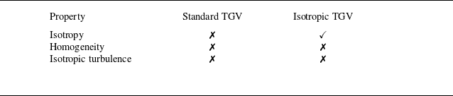
. Table 1 summarises the key properties of both cases. In addition, the supplementary material includes selected results for the standard and isotropic TGVs at
 $Re=3200$
obtained on a mesh consisting of
 $512^3$
nodes. These results are in very good agreement with all statements made in the paper, confirming the conclusions even after doubling the Reynolds number.
Selected properties of the standard and isotropic TGVs.

Lumley triangle for x–y-plane-averaged dissipation tensor as a function of
 $z/l_0$
at different times for the standard TGV (a) and the isotropic TGV (b).

Finally, to facilitate a clearer contextualisation of the results, data of forced homogeneous isotropic turbulence from the literature (Cardesa, Vela-Martín & Jiménez Reference Cardesa, Vela-Martín and Jiménez2017) were also analysed and included in the supplementary material. These data exhibit a much more homogeneous and isotropic behaviour than both TGV cases.
7. Summary
This study examined the isotropy and homogeneity of the standard and isotropic TGV configurations using high-order numerical simulations. Both flow configurations were analysed using classical statistical quantities that characterise turbulent flows, as well as the recently introduced homogeneity indices. The standard TGV, although widely used as a benchmark for turbulence modelling, exhibits persistent anisotropy and inhomogeneity even at late decay stages. In terms of integral length scales, the standard TGV is not isotropic; in addition the isotropic TGV does not satisfy the conditions of homogeneous isotropic turbulence. Both flow configurations display spatial inhomogeneities in the
 $z$
direction, with persistent peaks in the coherent structure function and the turbulent kinetic energy at
 $z/l_0=\pi /2,3\pi /2$
. These features originate from the symmetry of the initial conditions and are maintained by the triply periodic computational domain, through the symmetry-preserving properties of the Navier–Stokes equations, combined with the progressive reduction of nonlinear mixing during decay, which apparently prevents a fully homogeneous flow development. Based on the obtained data and the supplementary material, we do not observe evidence for an approach to homogeneity with increasing Reynolds number. In the formal limit of infinite Reynolds number (zero viscosity) and for sufficiently long integration times, it is conceivable that the accumulation of round-off errors may induce a transition to fully developed turbulence, which could eventually approach a state of homogeneous isotropic turbulence. Such behaviour would likely represent a numerical artefact rather than a manifestation of the underlying flow dynamics, which for any finite Reynolds number and time remains conditioned by the initial TGV state.
In summary, while the isotropic TGV provides a more balanced and symmetric test case, neither flow achieves true homogeneous isotropic turbulence. This should be kept in mind, in particular, when employing the standard TGV as a reference case for turbulence model validation or for isotropy-based assumptions.
Supplementary material
Supplementary material is available at https://doi.org/10.1017/jfm.2026.11380.
Acknowledgements
The authors gratefully acknowledge Poland’s high-performance computing infrastructure, including PLGrid, ACK Cyfronet AGH, and PCSS, for providing computational facilities and technical support.
Funding
A.T. acknowledges financial support from the statutory funds of the Czestochowa University of Technology under grant BS/PB 1-100-3010/2025/P. Computational resources were supported by PLGrid through grants PLG/2025/018864 and PL0356-01.
Declaration of interests
The authors report no conflict of interest.
Data availability statement
The datasets used and/or analysed during the current study are available from the corresponding author on reasonable request.
Author contributions
M.K., J.H. and M.G. contributed conceptualisation; A.T. performed the simulations; M.K. and A.T. post-processed the data; M.K. created the figures and wrote the manuscript; all authors reviewed the manuscript.
Appendix
This appendix provides several analytical results for the global statistical behaviour of the standard and isotropic TGVs for
 $t=0$
, as shown in table 2. The turbulent integral length scales for
 $t=0$
have been obtained by integrating up to the first zero crossing of the autocorrelation function, i.e. using the positive lobe convention.
Selected analytical results for global statistics at
 $t/t_0=0$
.








 Open access

