1. Introduction
Spin coating has gained significant prominence in recent years as one of the foremost methods employed in industry to produce coating films with precise thickness and desired functionality. Its widespread adoption extends to various fields, including microelectronics, optics and other scientific domains. For example, coating for antireflective film (Sarkın et al. Reference Sarkın, Ekren and Saglam2020) or physical protective film (Santoro et al. Reference Santoro, Venkateswaran, Amadeo, Zhang, Brioschi, Callanan, Agrifoglio, Banfi, Bradley and Pesce2018), recording CDs (Mahmoodi Reference Mahmoodi2023), patterning of lithographic process (Zhao et al. Reference Zhao, Song, Ren, Zhang, Lin and Zhao2022) and manufacturing of integrated circuits (Lopes et al. Reference Lopes, Santos, de Almeida and Tavakoli2021) are all inseparable from it. In these applications, it is critical to control the uniformity of coating films, and the early work by Emslie, Bonner & Peck (Reference Emslie, Bonner and Peck1958) has demonstrated that such control is possible when the behaviour and physical mechanisms of the spreading film become better understood.
The process of spin coating is typically carried out by placing a drop on a rotating substrate. Driven by centrifugal forces, the liquid spreads outwards in the radial direction in an approximately axisymmetric way, forming a thin film in the centre and a capillary ridge at the edge. The axisymmetric spreading was first investigated by Emslie et al. (Reference Emslie, Bonner and Peck1958), who employed the lubrication approximation to simplify the governing equations, and assumed that the flow is governed by the balance between centrifugal and viscous forces, while capillary forces can be neglected. Adopting the method of characteristics, the exact solution for the film evolution was obtained, indicating that a uniformly flat film is consistently achieved during the spinning coating process, irrespective of any given initial profile. In particular, the film thickness scales as
 $t^{-1/2}$
for large time
 $t$
, as verified by the experiment of Melo et al. (Reference Melo, Joanny and Fauve1989). Assuming a flat profile of the drop, an implementation of mass conservation condition suggests that the drop radius should evolve as
 $t^{1/4}$
(Melo et al. Reference Melo, Joanny and Fauve1989; Fraysse & Homsy Reference Fraysse and Homsy1994). However, this axisymmetric solution of the drop radius failed to agree quantitatively with the experimental measurements (Fraysse & Homsy Reference Fraysse and Homsy1994; Spaid & Homsy Reference Spaid and Homsy1997; Holloway et al. Reference Holloway, Habdas, Semsarillar, Burfitt and de Bruyn2007). The discrepancy between theory and experiment is attributed to the presence of a capillary ridge near the contact line, which, in contrast to the central region, is characterized by a finite curvature (Fraysse & Homsy Reference Fraysse and Homsy1994). Therefore, capillary forces play an important role and should not be neglected. This argument has been confirmed by the theoretical and numerical investigation of Wilson et al. (Reference Wilson, Hunt and Duffy2000), who considered the axisymmetric spreading of a drop in spin coating in the framework of lubrication theory. They show that the numerical solution of the lubrication equation with finite surface tension could well fit the experimental data of the drop radius (Fraysse & Homsy Reference Fraysse and Homsy1994; Spaid & Homsy Reference Spaid and Homsy1997), while the asymptotic solutions with no or sufficiently weak surface tension failed to exhibit a quantitative agreement.
In practical spin coating, the axisymmetric spreading occurs only at the early stage. When the radius of the drop gradually increases, the capillary ridge near the contact line becomes unstable, leading to a wavy rim and subsequent development of finger-like rivulets. This fingering instability has received a great deal of attention in the literature (see e.g. Melo et al. Reference Melo, Joanny and Fauve1989; Fraysse & Homsy Reference Fraysse and Homsy1994; Spaid & Homsy Reference Spaid and Homsy1997; Schwartz & Roy Reference Schwartz and Roy2004; Holloway et al. Reference Holloway, Habdas, Semsarillar, Burfitt and de Bruyn2007). Since the basic axisymmetric flow is time-dependent, a stringent stability analysis of spin coating is challenging. It is usually assumed that the capillary ridge evolves in a quasi-steady manner such that an analogy with the fingering instability of a gravity draining film down a plate can be adopted. For the latter, a capillary ridge also occurs near the advancing contact line (Huppert Reference Huppert1982; Tuck & Schwartz Reference Tuck and Schwartz1990; Moriarty et al. Reference Moriarty, Schwartz and Tuck1991), and a stability analysis based on normal modes can be performed (Troian et al. Reference Troian, Herbolzheimer, Safran and Joanny1989; Spaid & Homsy Reference Spaid and Homsy1996; Bertozzi & Brenner Reference Bertozzi and Brenner1997). Based on the linear stability theory of Troian et al. (Reference Troian, Herbolzheimer, Safran and Joanny1989), the number of fingers observed in the experiment of spin coating by Fraysse & Homsy (Reference Fraysse and Homsy1994) and Holloway et al. (Reference Holloway, Habdas, Semsarillar, Burfitt and de Bruyn2007) shows a satisfactory agreement, provided that the experimentally measured value of the critical drop radius at the onset of instability is given. We note that the fingering instability typically occurs well before the droplet is fully spread out. The ratio between the critical and initial radius is approximately less than 2 and insensitive to the angular velocity at low rotational rates (Melo et al. Reference Melo, Joanny and Fauve1989; Fraysse & Homsy Reference Fraysse and Homsy1994; Holloway et al. Reference Holloway, Habdas, Semsarillar, Burfitt and de Bruyn2007). The attainable radius of axisymmetric spreading can be increased by a few times when the rotation is sufficiently fast, as demonstrated experimentally by Wang & Chou (Reference Wang and Chou2001). Obviously, the presence of the capillary ridge is crucial in triggering the fingering instability. However, a systematic investigation of the evolution of the capillary ridge in spin coating remains to be performed.
Some insights of the instability of spin coating can be gained at low rotational speeds. In this situation, the profile of a partially wetting droplet admits a static solution, which is determined by the balance between capillary and centrifugal forces with a possible modulation of gravity. In the framework of lubrication theory, an analytical form of the solution was reported by McKinley and co-workers (McKinley et al. Reference McKinley, Wilson and Duffy1999; McKinley & Wilson Reference McKinley and Wilson2001, Reference McKinley and Wilson2002), who also investigated a mathematically equivalent problem, namely a sessile drop subject to an air jet acting normally to the substrate. McKinley et al. (Reference McKinley, Wilson and Duffy1999) show that some of the solutions may be stable to axisymmetric disturbances. However, a subsequent linear stability analysis demonstrated that all solutions are unconditionally unstable to non-axisymmetric disturbances (McKinley & Wilson Reference McKinley and Wilson2002). Schwartz & Roy (Reference Schwartz and Roy2004) also performed a stability investigation using an energy method, both with and without the lubrication approximation, and confirmed the unstable feature of the drop in spin coating. Boettcher & Ehrhard (Reference Boettcher and Ehrhard2014) assumed that the interface profile away from the contact line can be described by a quasi-static solution, in which the contact-angle condition may not be satisfied, and reported stability behaviours of a droplet under gravitational and centrifugal forces similar to McKinley & Wilson (Reference McKinley and Wilson2002). It remains unclear to what extent the unsteady droplet profile can be approximated by these quasi-static solutions. Definitely, while these static or quasi-static solutions may exhibit a convex or concave shape of the droplet, they do not describe the film profile near the onset of fingering instability at large rotational rates (Melo et al. Reference Melo, Joanny and Fauve1989), which is characterized by a well-flattened central region and an annular capillary ridge.
This paper focuses on the axisymmetric spreading and thinning of a Newtonian fluid in the framework of lubrication theory, aiming at a systematic description of the interface evolution. Particular attention is devoted to the contact-line dynamics and the evolution of the capillary ridge. At low rotational rates, we will present an asymptotic solution to describe the approaching of the drop profile toward the equilibrium state. When the droplet is spread out by centrifugal force, we report a novel film structure separating the central region and the capillary ridge, whose thickness scales with the contact-line speed
 $\dot {a}$
as
 $\dot {a}^{2/3}$
in analogy with the Landau–Levich–Derjaguin-type (LLD-type) film (Landau & Levich Reference Landau and Levich1942; Derjaguin Reference Derjaguin1943). The presence of this new region gives rise to the decoupling of the evolutions of the central region and the capillary ridge, in contrast to the classical scenario that the central flat film and the capillary ridge are directly connected, yielding a film thickness proportional to
 $t^{-1/2}$
.
The paper is organized as follows. The problem statement and governing equation are introduced in § 2, together with initial and boundary conditions. Numerical and theoretical results are presented in § 3. Starting from an overview of the flow regimes in § 3.1, the interface evolution at low rotational rates together with the static solution is presented in § 3.2, where a reduced equation for the drop radius is also derived using matched asymptotic expansions. In § 3.3, the characteristics of the central flat film, the capillary ridge and the LLD-type film are studied in a piecewise way; both numerical results and approximate theory are presented and discussed. Some conclusions are drawn in § 4.
2. Formulation
We consider a Newtonian drop with volume
 $V$
, which spreads on a rotating horizontal substrate with angular speed
 $\omega$
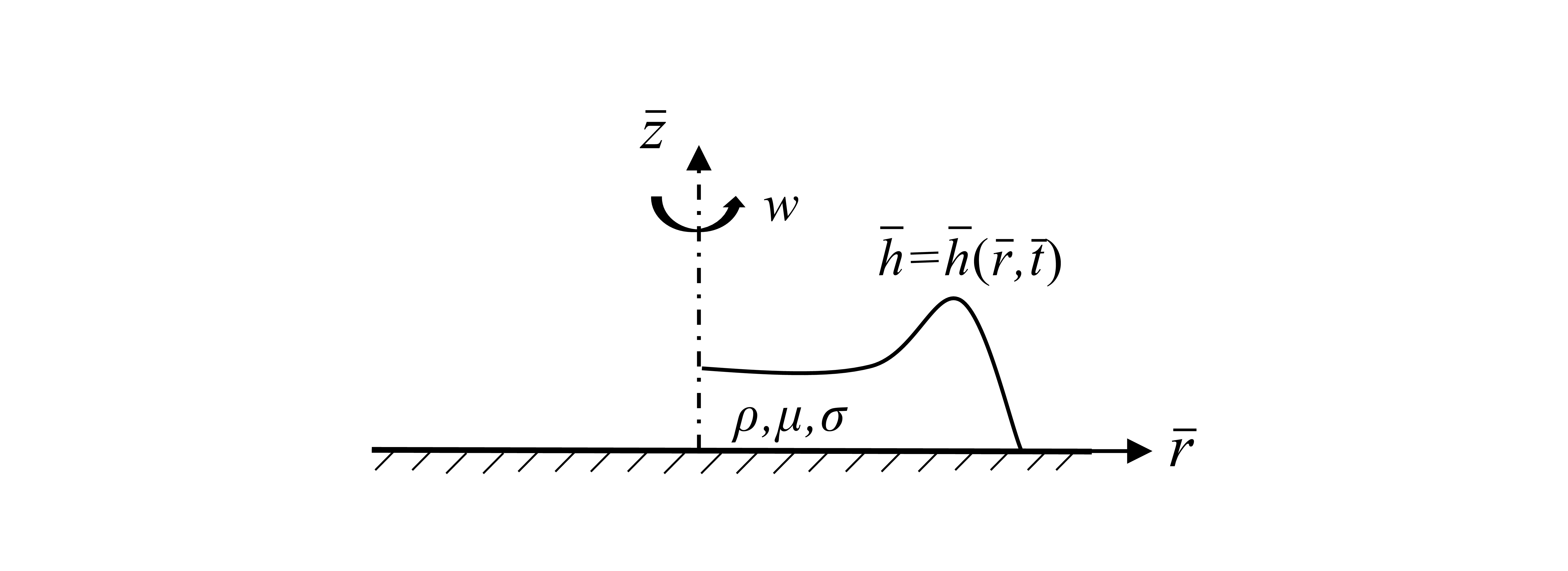
, as sketched in figure 1. The liquid is of constant viscosity
 $\mu$
and density
 $\rho$
, and the surface tension is denoted by
 $\sigma$
. It is convenient to introduce a cylindrical coordinate system
 $(\bar {r},\bar {\varphi }, \bar {z})$
; hereafter, we use a bar to denote dimensional variables. For the axisymmetric spreading of present interest, the position of the free surface is written as
 $\bar{z}=\bar {h}(\bar {r}, \bar {t})$
, where
 $\bar {t}$
denotes time. The surface of the drop intersects the substrate with a microscopic contact angle
 $\theta _e$
, which is assumed small such that the lubrication approximation can be used (Oron et al. Reference Oron, Davis and Bankoff1997). It is known that the presence of moving contact lines gives rise to a stress singularity (Huh & Scriven Reference Huh and Scriven1971; Dussan & Davis Reference Dussan and Davis1974), which should be resolved by introducing a microscopic contact-line model such as some sort of slip (Snoeijer & Andreotti Reference Snoeijer and Andreotti2013). Among others, the Greenspan slip model (Greenspan Reference Greenspan1978) can fully eliminate the contact-line singularity and is appropriate in numerically solving the lubrication equation, as employed by Wilson et al. (Reference Wilson, Hunt and Duffy2000) for the spin coating problem. In the present work, we alternatively adopted the Navier slip model, which is more popular in theoretical studies of moving contact lines (see e.g. Hocking Reference Hocking1983; Eggers Reference Eggers2005). The slip length is denoted by
 $\lambda _s$
, which is typically of a few nanometres.
Sketch of the thin film flow on a rotating horizontal substrate.

Initially, the drop maintains an equilibrium state without rotation. We define a length scale
 \begin{equation} L=\left (\frac {V}{2\pi \theta _{e}}\right )^{1/3}, \end{equation}
which measures the horizontal extent of the drop; one can easily verify that the maximum height of the equilibrium drop is given by
 $\theta _eL$
. The problem can be simplified by estimating the Ohnesorge number
 $Oh=\mu /\sqrt {\rho L\theta _e\sigma }$
, the Bond number
 $Bo=g\rho L^2\theta _e^2/\sigma$
and the reduced Reynolds number
 $Re=\rho \omega L^2\theta _e^2/\mu$
, which measure the ratios of viscous to inertia and capillary forces, gravity to capillary forces, and Coriolis to viscous forces, respectively. In particular, the estimation of the Coriolis force can be found in Emslie et al. (Reference Emslie, Bonner and Peck1958). Following Melo et al. (Reference Melo, Joanny and Fauve1989), Fraysse & Homsy (Reference Fraysse and Homsy1994) and Wilson et al. (Reference Wilson, Hunt and Duffy2000), we consider a small viscous drop such that
 $Oh\gg 1$
,
 $Bo\ll 1$
and
 $Re\ll 1$
. Then the evolution of the liquid film is governed by viscosity, capillarity and centrifugal force, while the effects of inertia, gravity and Coriolis forces can be neglected.
Then the problem is non-dimensionalized by scaling the variables as
 \begin{equation} \bar {r}=Lr,\quad \bar {h}=\theta _{e}Lh,\quad \bar {t}=\frac {3\mu L}{\sigma \theta ^{3}_{e}}\,t. \end{equation}
Accordingly, the lubrication equation governing the axisymmetric spin coating can be written in dimensionless form as
 \begin{equation} h_{t}+\frac {1}{r}\left \{rh^{2}\left (h+3\lambda \right )\left [\left (\frac {\left (rh_{r}\right )_{r}}{r}\right )_{r}+\beta r\right ]\right \}_{r}=0, \end{equation}
where the rotational Bond number
 \begin{equation} \beta =\frac {\rho \omega ^{2}V}{2\pi \sigma \theta _{e}^2} \end{equation}
measures the ratio of centrifugal force and surface tension, and is the sole parameter containing the angular speed
 $\omega$
;
 $\lambda =\lambda _s/(\theta _{e}L)$
is the dimensionless slip length.
The fourth-order equation (2.3) is supplemented by the following conditions. At the axis
 $r=0$
, we have the symmetry conditions
 \begin{equation} h_{r}=0,\quad h_{rrr}=0. \end{equation}
The boundary conditions at the contact line
 $r=a(t)$
are
 \begin{equation} h=0,\quad h_{r}=-1. \end{equation}
Since the contact-line radius
 $a(t)$
should be solved as part of the solution, an additional condition is required. It turns out to be a kinematic condition, i.e.
 \begin{equation} \dot a =3\lambda \lim _{r\to a} hh_{rrr}, \end{equation}
where
 $\dot {a}\equiv \mathrm {d}a/\mathrm {\rm d}t$
represents the contact-line velocity. This condition can be obtained by calculating the depth-averaged velocity of the liquid and then taking the limit towards the contact line. The initial condition is simply an equilibrium drop, which has a parabolic profile and reads
 \begin{equation} h(r,0)=1-\frac {r^{2}}{4}. \end{equation}
Note that the initial radius of the contact line is
 $a(0)=2$
. Besides, by integrating (2.3), one can easily demonstrate that the mass conservation condition
 \begin{equation} \int _{0}^a rh \,\mathrm {\rm d}r=1 \end{equation}
is automatically satisfied.
The axisymmetric lubrication equation (2.3) and the complementary conditions (2.5)–(2.8) were solved numerically using an algorithm presented in Qin et al. (Reference Qin, Lu and Gao2024). The main ingredients of the method are also described in Appendix A for completeness.
3. Results
The spin coating is governed by two parameters, i.e.
 $\beta$
and
 $\lambda$
. It is expected that
 $\lambda$
plays a logarithmic role in the macroscopic film profiles. Our numerical results show that the film evolution at
 $\lambda =10^{-4}$
and
 $10^{-5}$
does not exhibit qualitative differences. In the present work, a rather small slip length
 $\lambda =10^{-5}$
is implemented; this value is reasonable for a millimetre-sized drop. We focus on the effect of the rotational Bond number
 $\beta$
on the film evolution.
Interface evolution for different values of
 $\beta$
: (a)
 $\beta =0.5$
at
 $t=0$
, 5, 10, 15, 100; (b)
 $\beta =1$
from
 $t=0$
to
 $t=900$
with time interval
 $100$
; (c)
 $\beta =4$
from
 $t=0$
to
 $t=180$
with time interval
 $20$
. The insets in (b) and (c) show the details of the film near the ridge.

3.1. Overview of film evolution
Our numerical results show that the spreading of the drop on a rotational substrate develops into different interfacial shapes depending on the spin rates. As depicted in figure 2, we begin with an overview of the evolution of the film profiles and their dependence on the governing parameter
 $\beta$
. As shown later, there exists a critical value of rotational Bond number,
 $\beta _c=3/4$
, which separates two distinct flow regimes in film evolution. When
 $\beta \leqslant \beta _c$
, the lubrication equation admits a static solution, corresponding to a balance between capillary and centrifugal forces. As shown in figure 2(a) for
 $\beta =0.5$
, the initial droplet spreads under the influence of centrifugal force and eventually approaches the static solution. The equilibrium position of the contact line remains close to its initial position. In contrast, when
 $\beta \gt \beta _c$
, the drop continues to spread, giving rise to a thin liquid film, as illustrated in figure 2(b,c). The film becomes thinner with time and is characterized by a flat film in the central region and a capillary ridge near the contact line. For convenience, the film evolutions for
 $\beta$
below and above
 $\beta _c$
are referred to as the low-speed and high-speed regimes, respectively. Notably, in the high-speed regime, when
 $\beta$
is slightly above
 $\beta _c$
, a thinner film occurs between the central flat film and the capillary ridge, as shown in figure 2(b) for
 $\beta =1$
. This film was identified as an LLD-type film (Landau & Levich Reference Landau and Levich1942; Derjaguin Reference Derjaguin1943), which is entrained by the displacement of the capillary ridge. Note that the LLD-type film disappears after a finite period of time. When
 $\beta$
is significantly larger than
 $\beta _c$
, the LLD-type film was not observed, with the central region directly connected to the capillary ridge (see figure 2(c) for
 $\beta =4$
). More detailed elaboration of each regime will be presented in the following subsections.
3.2. Low-speed regime
3.2.1. Existence of a static solution
The static solution describing the morphology of a thin drop driven by centrifugal forces in spin coating or by a jet of impinging air was reported by McKinley et al. (Reference McKinley, Wilson and Duffy1999), McKinley & Wilson (Reference McKinley and Wilson2002) and Schwartz & Roy (Reference Schwartz and Roy2004). In terms of present dimensionless variables, the solution without gravity can be written as
 \begin{equation} h=\frac {\left (a^{2}_{\infty }-r^{2}\right )\left [16-\beta a_{\infty }\left (a^{2}_{\infty }-r^{2}\right )\right ]}{32a_{\infty }}, \end{equation}
which can also be derived from the lubrication equation (2.3) together with the boundary conditions (2.5) and (2.6). Here,
 $a_\infty$
is the radius of the contact line, which is also the limit of the contact-line radius as
 $t$
goes to infinity in the low-speed regime. According to the volume conservation condition (2.9),
 $a_\infty$
can be determined as
 \begin{equation} a_{\infty }=\left [\frac {4}{\beta }\left (3\pm \sqrt {9-12\beta }\right )\right ]^{1/3}. \end{equation}
Clearly, the solution exists only when
 $\beta \leqslant \beta _c=3/4$
.
The relationship between
 $a_\infty$
and
 $\beta$
is plotted in figure 3(a). It is seen that the solution bifurcates at
 $\beta =\beta _c$
, giving rise to two branches of the curve. The lower and upper branches of the solution are expected to be stable and unstable to axisymmetric disturbances, respectively. Therefore, it is only the lower branch of the solution that can be realized in our axisymmetric calculations. Representative drop profiles of the static solution are presented in figure 3(b). As
 $\beta$
increases along the lower branch, the drop height is significantly reduced, while the contact-line radius increases by a relatively small amount. At the threshold, the contact-line radius for the lower branch attains its maximum
 $a_{c,\infty }=2^{4/3}$
, and the corresponding drop profile is given by the red curve in figure 3(b). There is another critical point,
 $\beta =2/3$
, beyond which the drop is concave around the axis. When
 $\beta \lt 2/3$
, the solution of the upper branch exhibits negative film thickness and hence is unphysical.
(a) Bifurcation curves of the static solution in terms of
 $a_\infty$
as functions of
 $\beta$
. The solid and dashed lines correspond to the negative and positive signs in (3.2), respectively. (b) Static drop profiles given by (3.1) for representative values of
 $\beta$
. The solid and dashed lines correspond to the lower and upper branches in (a), respectively.

The static solution is compared with the numerical results of the unsteady lubrication equation in figure 4 for
 $\beta =0.5$
and 0.7. In both cases, the numerical solution converges to an equilibrium state. For sufficiently large times, e.g.
 $t=100$
, the interface profiles show perfect agreement with the static solution denoted by the dashed lines. This comparison in turn demonstrates the accuracy of our numerical algorithm.


3.2.2. Asymptotic solution of low-speed drop spreading
When
 $\beta \leqslant \beta _c$
, the drop is expected to spread at a rather slow rate, i.e.
 $\dot {a}\ll 1$
. An asymptotic theory can be developed in the limit
 $\lambda \rightarrow 0$
following the procedure proposed by Hocking (Reference Hocking1983), who considered the spreading of a thin drop in the absence or presence of gravity. For the present spin coating problem, the structure of the drop consists of an outer region and an inner region near the contact line. In the outer region, the drop exhibits a quasi-static behaviour and the slip effect is insignificant. The inner region is characterized by a length of
 $O(\lambda )$
, over which a significant variation of the surface slope occurs due to the large viscous force therein. A matching of the outer and inner solutions typically yields a relation between the speed and position of moving contact lines.
For the outer solution, it is instructive to replace
 $r$
with the new variable
 $y=r/a$
. Accordingly, the problem is transformed onto a fixed domain
 $0\leqslant y\leqslant 1$
. Then the lubrication equation of
 $h=h(y,t)$
can be written as
 \begin{equation} h_{t}-\frac {\dot {a}}{a}yh_y+\frac {1}{a^4y}\left \{yh^{3}\left [\left (\frac {\left (yh_{y}\right )_{y}}{y}\right )_{y}+\beta a^4y\right ]\right \}_{y}=0, \end{equation}
where the slip effect has been neglected. The supplementary conditions include
 \begin{equation} h_y=0,\ h_{yyy}=0 \quad \mbox {at}\ y=0, \end{equation}
 \begin{equation} h=0 \quad \mbox {at}\ y=1, \end{equation}
and the condition of the mass conservation
 \begin{equation} \int _{0}^1 yh \,\mathrm {d}y=a^{-2}. \end{equation}
Note that it is unnecessary for the outer solution to satisfy the contact-angle condition.
When the contact-line velocity
 $\dot {a}$
is small, it turns out that
 $h$
can be expanded as
 \begin{equation} h(y,t )=h_{0} (y,a )+\dot {a}\,h_{1} (y,a )+O(\dot {a}^{2}), \end{equation}
where
 $h_0$
and
 $h_1$
represent the hydrostatic profile and the first-order correction by the flow, respectively. Accordingly, the time derivative in (3.3) can be expressed as
 \begin{equation} h_{t}=\dot {a} h_{0a}+O(\dot {a}^{2}). \end{equation}
Substituting (3.7) and (3.8) into (3.3), we obtain equations for each power of
 $\dot {a}$
. The leading-order equation, after one integration, reads
 \begin{equation} \left [\frac {\left (yh_{0y}\right )_{y}}{y}\right ]_{y}+\beta a^{4}y=0. \end{equation}
The solution is given by
 \begin{equation} h_{0}=\frac {\left (1-y^{2}\right )\left [4-2b\left (1-3y^2\right )\right ]}{a^{2}}, \end{equation}
where
 $b=\beta a^{6}/{192}$
. This quasi-static solution satisfies boundary conditions in the form of (3.4)–(3.6) with
 $h$
replaced by
 $h_0$
. One can easily verify that (3.10) reduces to the equilibrium solution (3.1) when
 $a=a_\infty$
given by (3.2). The first-order correction is determined by the equation
 \begin{equation} h_{0a}-\frac {y}{a}h_{0y}+\frac {1}{a^{4}y}\left \{yh_{0}^{3}\left [\frac {\left (yh_{1y}\right )_{y}}{y}\right ]_{y}\right \}_y=0. \end{equation}
The details of solving (3.11) for
 $h_{1}$
are given in Appendix B. Of present interest is the slope close to the contact line. Correspondingly, we have
 \begin{equation} h_{1y}\left (y\right )\sim -\frac {a^7}{64\left (1+b\right )^{2}}\left \{\ln \left [\mathrm {e}^2\,\frac {2-b}{1+b}\left (1-y\right )\right ]-\frac {3b}{4-2b}\right \}\quad \mbox {as}\ y\rightarrow 1. \end{equation}
It is convenient to calculate the cube of the surface slope, which can be directly matched by the inner solution without invoking an intermediate region (Eggers Reference Eggers2005; Savva & Kalliadasis Reference Savva and Kalliadasis2009; Sibley et al. Reference Sibley, Nold and Kalliadasis2015; Savva et al. Reference Savva, Rezgdnikov and Colinet2017). Combining (3.12) and the derivative of (3.10), we obtain
 \begin{eqnarray} h_{y}^{3} & =& h_{0y}^{3}+3\dot {a}h_{0y}^{2}h_{1y}+O (\dot {a}^{2} ) \nonumber \\ & \sim & -\left [\frac {8(1+b)}{a^{2}}\right ]^{3}-3a^{3}\dot {a}\left \{\ln \left [\mathrm {e}^{2}\,\frac {2-b}{1+b}\left (1-y\right )\right ]-\frac {3b}{4-2b}\right \}\quad \mbox {as}\ y\rightarrow 1. \end{eqnarray}
Since this solution does not satisfy the contact-angle condition, there must be an inner region, where the slip effect should be taken into account.
For the inner solution, we consider a small-
 $\dot {a}$
expansion again, just as for the outer region:
 \begin{equation} H (\xi ,t )=H_{0} (\xi ,a )+\dot {a}\,H_{1} (\xi ,a )+O(\dot {a}^{2}), \end{equation}
where
 $H=h/(3\lambda )$
and
 $\xi = (a-r )/{(3\lambda )}$
. The inner solution has been solved in many papers (Hocking Reference Hocking1983; Eggers Reference Eggers2005; Sibley et al. Reference Sibley, Nold and Kalliadasis2015). The asymptotic behaviour of the solution for large
 $\xi$
is
 \begin{equation} H_{\xi }=1+\dot {a}\ln (\mathrm {e}\xi )+O (\dot {a}^{2}). \end{equation}
Furthermore, the cube of
 $H_\xi$
has the form
 \begin{equation} H^{3}_{\xi }=1+3\dot {a}\ln (\mathrm {e}\xi )+O (\dot {a}^{2}), \end{equation}
which can be matched with the outer solution.
Rewriting the inner solution (3.16) using the outer variables
 $h$
and
 $y$
, and matching to the outer solution (3.13), we obtain a relation between
 $a$
and
 $\dot {a}$
:
 \begin{equation} \left [\frac {8(1+b)}{a^{3}}\right ]^{3}-1=3\dot {a}\left [\ln \left (\frac {1+b}{2-b}\,\frac {a}{3\mathrm {e}\lambda }\right )+\frac {3b}{4-2b}\right ]. \end{equation}
Note that
 $b\leqslant 1$
is satisfied in the low-speed regime such that the argument of the logarithmic term remains positive. The left-hand side of (3.17) represents the cube difference between the apparent and equilibrium contact angles. To validate (3.17), we explore two special cases. First, when
 $\dot {a}=0$
, it is trivial to show that the contact-line position of the static solution, i.e. (3.2), is recovered. Second, considering the case
 $b=0$
, (3.17) reduces to
 \begin{equation} \left ( \frac {2}{a}\right )^{9}-1=3\dot {a}\ln \left (\frac {a}{6\mathrm {e} \lambda }\right ), \end{equation}
which is exactly the relation presented by Hocking (Reference Hocking1983) for drop spreading without centrifugal and gravitational forces.


The asymptotic solution of
 $a$
and
 $\dot {a}$
can be calculated conveniently by solving (3.17), starting from the initial value
 $a=2$
. The results for representative values of
 $\beta$
are shown in figure 5, where the numerical solutions of the lubrication equation (2.3) are also plotted for comparison. It can be seen that the asymptotic theory is in perfect agreement with the numerical results when
 $\beta \lt 3/4$
, since the underlying assumption of the asymptotic analysis, i.e.
 $\dot {a}\ll 1$
, does hold according to these results. We also observe that drops at larger values of
 $\beta$
move faster, but take longer to reach equilibrium.
Furthermore, it is noteworthy that the derivation of (3.17) does not rely on the condition
 $\beta \leqslant \beta _c$
. When
 $\beta$
slightly exceeds
 $3/4$
, the early stage of spreading is also quasi-static and (3.17) remains valid, as confirmed in figure 5 for
 $\beta =0.8$
and 1. The predictions of the quasi-static analysis deviate from the exact solutions for large
 $t$
due to the formation of thin films around the axis, as discussed later.
3.3. High-speed regime
In the high-speed regime (
 $\beta \gt 3/4$
), the drop continues to spread. The numerical results presented in figures 2(b,c) reveal that the film evolution goes through distinct stages. At the very late stage, the film ultimately evolves into a flat film zone surrounded by a capillary ridge. However, before reaching this final configuration, an LLD-type film zone can be developed when
 $\beta$
is slightly greater than
 $\beta _c$
(figure 2
b). At sufficiently large values of
 $\beta$
, the LLD-type film is not observed. Given the occurrence of these diverse film structures, the film evolution in different zones is governed by different physical mechanisms and can be studied in a piecewise manner, yielding local self-similarity solutions or scaling laws. In the following subsubsections, we examine the characteristics of the central flat film, the capillary ridge and the LLD film, including their mutual dependencies.
3.3.1. Flat central film
Figures 2(b,c) demonstrate that the film in the central zone flattens rapidly upon the application of rotation. Given the near-uniform thickness of the film, the curvature and hence the capillary force can be safely neglected in this region. Consequently, the flow is primarily governed by the balance between viscous and centrifugal forces. Eliminating the surface tension term and the slip effect, the lubrication equation (2.3) becomes
 \begin{equation} h_{\tau }+\frac {1}{r}\left (r^{2}h^{3}\right )_{r}=0. \end{equation}
We have introduced a rescaled time
 $\tau =\beta t$
, which scales out the surface tension according to (2.2) and (2.4). Emslie et al. (Reference Emslie, Bonner and Peck1958) and Schwartz & Roy (Reference Schwartz and Roy2004) solved (3.19) under initial conditions of a general form and a uniform film, respectively. In particular, given an initially uniform film of thickness
 $h_p$
, the solution is
 \begin{equation} h_{f}=\frac {h_p}{\sqrt {1+4h_p^2\tau }}, \end{equation}
which describes the thinning of a flat film with thickness
 $h_f$
. The long-time asymptotics of these solutions has the form
 \begin{equation} h_{f}=\tfrac {1}{2}\tau ^{-{1}/{2}}, \end{equation}
and has also been reported by Fraysse & Homsy (Reference Fraysse and Homsy1994). It is trivial to verify that (3.21) is a self-similar solution of (3.19). Clearly, as initial and boundary conditions are not involved, this solution holds for long-time evolution of the film and is independent of the film structure near the contact line. The comparison of the numerical results and the theoretical solution (3.21) is depicted in figure 6. It can be seen that the numerical results for all values of
 $\beta$
collapse onto the theoretical curve at large
 $\tau$
. According to (3.20), the range of
 $\tau$
over which the data approach the similarity solution depends on
 $h_p$
rather than
 $\beta$
. However, for the initial condition of a drop profile, the timescale for the collapse depends on
 $\beta$
; as shown in the inset of figure 6, it takes a longer time to approach the theoretical curve for smaller
 $\beta$
. We emphasize that surface tension still plays a role in the early surface evolution due to the finite curvature, and can only be disregarded as the liquid film is well flattened. As shown in figure 6, deviations of the numerical results from the theoretical curve can be observed at the early stage due to the effect of surface tension, especially for small values of
 $\beta$
.


3.3.2. Capillary ridge
An annular ridge occurs in the vicinity of the contact line such that capillary force becomes locally important. The ridge is connected to the LLD-type film (figure 2
b) or the thin flat film zone (figure 2
c), depending on the spinning rate and time stage. We first discuss the case without the LLD-type film. Figure 7(a) shows the film profiles at
 $\beta =2$
and four time instants when the flat film and the ridge are well developed. As the film spreads, both the thickness of the flat region and the height and width of the ridge decrease. The relative height of the ridge with respect to the thickness of the flat region actually grows with time, as shown in the inset of figure 7(a). The influence of
 $\beta$
on the ridge size is depicted in figure 7(b), which plots the film profiles at a given
 $\tau$
, corresponding to an approximately identical value of
 $h_f$
. As demonstrated later, the shape of the ridge is determined by the balance between capillary and centrifugal forces. With an increase in
 $\beta$
, the centrifugal force becomes more pronounced. Therefore, the ridge size is reduced such that the capillary force increases to balance the centrifugal force.
(a) Instantaneous film profiles at
 $\beta =2$
. The inset shows the local structures of the capillary ridge with
 $h$
rescaled by
 $\tau ^{-1/2}$
or equivalently the thickness of the flat region. (b) The ridge profiles for different
 $\beta$
at
 $\tau =600$
.

It is believed that the capillary ridge in spin coating evolves in a quasi-steady way, similar to the two-dimensional ridge encountered in the front of a draining film on a wall (Troian et al. Reference Troian, Herbolzheimer, Safran and Joanny1989; Fraysse & Homsy Reference Fraysse and Homsy1994). The present calculations allow for more quantitative validation of this analogy. When the film is well spread out, the width of the capillary ridge
 $W$
is much smaller than the contact-line radius
 $a$
. Therefore, the local film around the ridge can be treated effectively as a two-dimensional region, in which the spatial variation of the driving centrifugal force can be neglected. Moreover, as the contact-line speed is small (see figure 10b), the evolution of the ridge is quasi-steady in a reference frame moving with the contact line. Accordingly, introducing
 $x=r-a$
, one gets an equation governing the film thickness in the ridge zone:
 \begin{equation} \frac {1}{\beta }h_{xxx}=\frac {a_{\tau }}{h\left (h+3\lambda \right )}-a, \end{equation}
where
 $a_{\tau }=\mathrm {d}a/\mathrm {d}\tau =\dot {a}/\beta$
is the rescaled contact-line velocity, and the three terms represent capillary, viscous and centrifugal forces, respectively. For
 $\lambda \ll 1$
, (3.22) possesses the solution of uniform thickness
 \begin{equation} h=\sqrt {\frac {a_{\tau }}{a}}. \end{equation}
It is convenient to rescale this equation by introducing
 \begin{equation} x=\left (\frac {a_{\tau }}{\beta ^{2}a^{3}}\right )^{1/6}X, \quad h=\sqrt {\frac {a_{\tau }}{a}}\,\mathcal {H},\quad \lambda =\sqrt {\frac {a_{\tau }}{a}}\,\Lambda , \end{equation}
which gives rise to
 \begin{equation} \mathcal {H}_{XXX}=\frac {1}{\mathcal {H}\left (\mathcal {H}+3\Lambda \right )}-1. \end{equation}
The boundary conditions are
 $\mathcal {H}(0)=0$
,
 $\mathcal {H}_X(0)=-1/\sqrt [3]{\beta a_{\tau }}$
and
 $\mathcal {H}\rightarrow 1$
as
 $X\rightarrow -\infty$
for
 $\Lambda \ll 1$
by ignoring higher-order
 $O(\Lambda )$
terms. Equations of similar forms have also been investigated by Tuck & Schwartz (Reference Tuck and Schwartz1990) and Spaid & Homsy (Reference Spaid and Homsy1996). A shooting method is employed to solve (3.25), with
 $a_\tau$
provided by the numerical solution of the full lubrication equation (2.3). As illustrated in figure 8, the quasi-steady theory agrees well with the numerical results. In particular, the asymptotically flat film of the ridge coincides with the central region and adapts to its decreasing thickness. The rescaled slip length
 $\Lambda$
plays only a weak role in the height of the ridge. As the film spreads, the increase of the maximum height of the ridge relative to the flat film, shown in the inset of figure 7(a), is caused by the slowing down of the contact-line speed, which results in an increase of the rescaled contact angle
 $1/\sqrt [3]{\beta a_{\tau }}$
.


(a) Evolution of the ridge volume for different
 $\beta$
. (b) Variation of the ridge volume as a function of
 $\beta$
at
 $\tau =5000$
, with the solid curve from (3.30). The inset illustrates a comparison of the ridge profiles, with the solid and dashed curves denoting the numerical solution and (3.28) at
 $\beta =6$
, respectively.

Furthermore, the quasi-steady model of the capillary ridge allows us to develop an approximate prediction of the macroscopic morphology of the ridge and the amount of liquid accumulated in it. At small spreading rates, the viscous flow is important only in the region of small film thicknesses, i.e. the thin flat film and the region near the contact line. Alternatively, the macroscopic shape of the ridge is determined mainly by the balance between the capillary and centrifugal forces. By neglecting the viscous term in (3.22), we have
 \begin{equation} h_{xxx}=-\beta a. \end{equation}
The thickness of the capillary ridge should vanish at the contact line. On the other side, the ridge connects to a flat film with an asymptotically vanishing thickness. Correspondingly, the boundary conditions of (3.26) have the form
 \begin{equation} h|_{x=-W}=0, \quad \frac {\partial h}{\partial x}\bigg |_{x=-W}=0, \quad h|_{x=0}=0, \quad \frac {\partial h}{\partial x}\bigg |_{x=0}=-1, \end{equation}
where the ridge width
 $W$
is defined as the distance from the dimple (see figure 8) to the contact line, and remains to be determined. Note that we simply impose
 $h_x=-1$
at
 $x=0$
, which is used as an additional condition to determine
 $W$
. This condition is based on the fact that the contact speed is small in the late stage, hence the apparent contact angle of the ridge remains close to the equilibrium contact angle, as confirmed by our numerical calculations. The solution to problem (3.26)–(3.27) can be readily obtained as
 \begin{equation} h=-\frac {\beta a}{6}x\left (x+W\right )^{2}, \quad W =\sqrt {\frac {6}{\beta a}}. \end{equation}
Correspondingly, the maximum height of the ridge is
 \begin{equation} h_{ridge} = \frac {4}{9}\sqrt {\frac {2}{3\beta a}}, \end{equation}
and the volume of the ridge can thus be calculated as
 \begin{equation} V_{ridge}=\int _{a-W}^a r h\,\mathrm {d}r\approx \int _{-W}^0 a h\,\mathrm {d}x=\frac {1}{2\beta }. \end{equation}
Interestingly,
 $V_{ridge}$
approaches a finite constant instead of vanishing after a long time. This scenario is confirmed by the numerical results shown in figure 9(a). Here,
 $V_{ridge}$
is computed by integrating from the local minimum between the flat region and the ridge to the contact line. It is seen that
 $V_{ridge}$
decreases with time, and varies very little in the late stages. The volume of the ridge at a large time instant
 $\tau =5000$
is plotted in figure 9(b) as a function of
 $\beta$
, and compares satisfactorily with the theoretical prediction (3.30). The agreement is due to a reasonable description of the ridge profile provided by (3.28), as illustrated in the inset of figure 9(b). Note that the capillary ridge can accommodate a significant amount of liquid at small
 $\beta$
.
Previous works on spin coating usually neglect the presence of the capillary ridge and assume a uniformly flat film to predict the growth of the contact radius (Emslie et al. Reference Emslie, Bonner and Peck1958; Fraysse & Homsy Reference Fraysse and Homsy1994). As a result, the volume conservation condition can be expressed as
 $a^2h_f=1$
, which, together with (3.21), yields the long-time asymptotics of the contact line:
 \begin{equation} a=2\tau ^{1/4},\quad a_{\tau }=\tfrac {1}{2}\tau ^{-3/4}. \end{equation}
In figure 10, we present a comparison of the theoretical and numerical solutions for different
 $\beta$
. The observed kinks in the curves for
 $\beta =0.8$
and
 $\beta =1$
are attributed to the appearance of LLD-type film, which will be discussed in § 3.3.3. The numerical results for
 $a$
are significantly below the values predicted by (3.31), especially for small values of
 $\beta$
. The deviation from the theoretical curve for the contact-line speed can also be observed in figure 10(b). The over-prediction of the theory was also observed in the work of Fraysse & Homsy (Reference Fraysse and Homsy1994), who reported an improved solution based on (3.20); however, there is still a remarkable deviation from their experimental results (see also Spaid & Homsy Reference Spaid and Homsy1997; Holloway et al. Reference Holloway, Habdas, Semsarillar, Burfitt and de Bruyn2007). These expressions can be improved by reconsidering the volume conservation condition, but with the volume of the capillary ridge subtracted. It turns out that the resulting radius and speed of the contact line differ from (3.31) only by a factor, and read
 \begin{equation} a=2\tau ^{1/4}\sqrt {1-\frac {1}{2\beta }},\quad a_{\tau }=\frac {1}{2}\tau ^{-3/4}\sqrt {1-\frac {1}{2\beta }}. \end{equation}
The numerical results are rescaled according to (3.32) and plotted in figure 11, which shows much better agreement between theory and calculations. The remaining difference at
 $\beta =0.8$
and
 $\beta =1$
is due to the occurrence of the LLD-type film, which is described later.


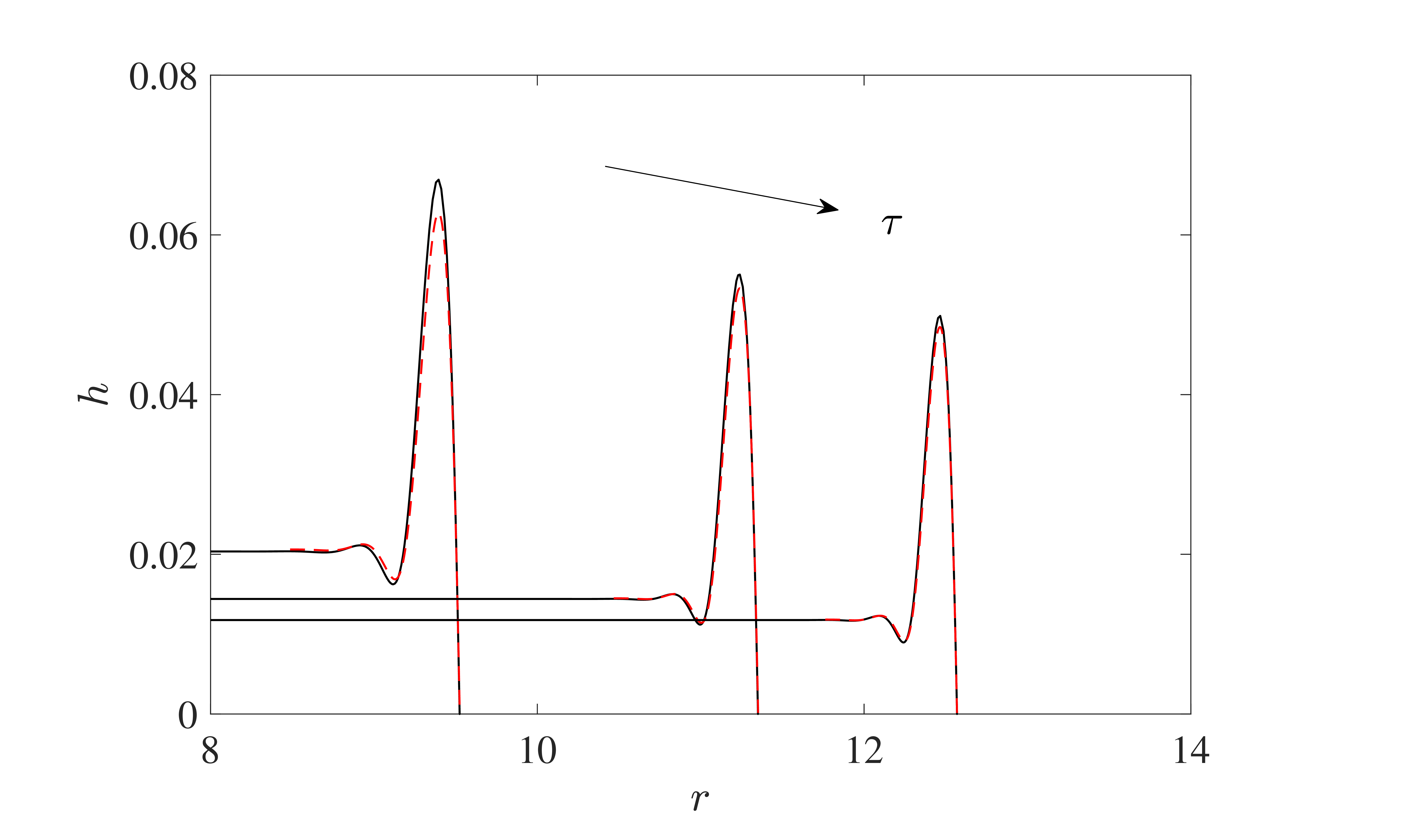
Evolution of the LLD-type film from
 $\tau =1000$
to
 $\tau=5000$
with time interval
 $1000$
for
 $\beta =0.8$
.

3.3.3. LLD-type film
As mentioned earlier, the flat central film is connected to the capillary ridge through an intermediate film zone when
 $\beta$
is slightly larger than
 $\beta _c$
. The thin film between the central region and the capillary ridge is further illustrated in figure 12 for
 $\beta =0.8$
. Compared with the central region, this intermediate film exhibits a couple of distinct features. First, its thickness is much smaller yet non-uniform. Second, a careful examination of figure 12 shows that the film thickness in the intermediate zone decreases with
 $r$
rather than time
 $\tau$
. The film profile varies from the flat central region to the thinner film through a smooth zone at
 $\tau =1000$
, which subsequently becomes steeper and evolves into a moving capillary shock. Meanwhile, the capillary ridge slows down. The thinner film eventually disappears at
 $\tau =5000$
due to the reconnecting of the flat film and the ridge, which is also responsible for the fluctuations of the curves in figures 10(b) and 11(b). Then the whole film evolves following the principles described earlier.
The presence of the thinner film and the capillary shock is reminiscent of the film structures in dip coating (Snoeijer et al. 2006; Gao et al. Reference Gao, Li, Feng, Ding and Lu2016; Xia et al. Reference Xia, Qin and Gao2020). A thin film can be entrained by withdrawing a solid plate away from a liquid bath, as first investigated by Landau & Levich (Reference Landau and Levich1942) and Derjaguin (Reference Derjaguin1943). We anticipate that the film in the intermediate region is entrained from the travelling capillary ridge following a similar mechanism, and hence refer to it as the LLD-type film. In order to confirm this idea and to develop a theoretical prediction of the film thickness, we examine the dynamic meniscus connecting the LLD-type film and the capillary ridge. The dynamic meniscus is assumed to move with the speed of the contact line. Employing the reference frame for analysing the capillary ridge, the film profile near
 $x=-W$
is governed by
 \begin{equation} h_{xxx} = \frac {\dot {a}}{h^2}\left ({1-\frac {h_L}{h}} \right ), \end{equation}
where
 $h_L$
is the thickness of the thin film with its weak non-uniformity neglected. The meniscus is governed by the balance between viscous and capillary forces, and the centrifugal force has also been neglected. Equation (3.33) is known as the Landau–Levich equation, and can be further simplified by appropriately rescaling the variables. As shown in many works (e.g.Landau & Levich Reference Landau and Levich1942; Wilson Reference Wilson1982; Du & Gao Reference Du and Gao2022), the solution for
 $h\gg h_L$
has an asymptotically constant curvature
 \begin{equation} h''_{in} = 0.643\frac {\dot {a}^{2/3}}{h_L}, \end{equation}
which should be matched to an outer solution corresponding to the macroscopic geometry of the capillary ridge. According to (3.28), the curvature of the capillary ridge as
 $x\rightarrow -W$
is
 \begin{equation} h''_{out} = \sqrt {\frac {2}{3}\beta a}. \end{equation}
The matching of the two curvatures yields
 \begin{equation} h_{L}=0.643\times \sqrt {\frac {3}{2\beta a}}\,\dot {a}^{2/3}, \end{equation}
which is confirmed by the numerical solution of the lubrication equation in figure 13. Here, the numerical results for
 $h_L$
are measured at the local minimum of the film. Due to the time-dependent contact-line velocity and radius, the LLD-type film becomes progressively thinner in thickness, distinguishing it from the classical LLD film.
Comparison of LLD-type film thickness with the asmptotic theory (3.36) at
 $\beta =1$
.

Since the LLD-type film is much thinner, it is expected that the flow rate in this zone is significantly suppressed. Consequently, the flat central film and the capillary ridge are decoupled and evolve independently, in contrast to the situations in the absence of the LLD-type film.
4. Concluding remarks
We have performed a numerical and theoretical investigation on the axisymmetric evolution of the liquid films on a rotating substrate, which is characterized by a small yet finite contact angle. The contact-line singularity is relieved by employing a Navier slip model with a sufficiently small slip length. Starting from an equilibrium state without rotation, a drop evolves into a new static solution when the rotational Bond number
 $\beta \leqslant 3/4$
. The drop spreading process can be well described by the solution based on matched asymptotic expansions. In particular, the asymptotic solution returns to the well-known solution of Hocking (Reference Hocking1983) when centrifugal force is absent. When
 $\beta \gt 3/4$
, the drop spreads into a liquid film driven by the centrifugal forces. In most situations, the film consists of a central region of uniform thickness and an annular capillary ridge. While the central film thins as
 $\tau ^{-1/2}$
, the height of the ridge decays at a much slower rate. It is found that the ridge follows a quasi-steady evolution, and the total volume of the ridge eventually approaches a constant
 $1/(2\beta )$
. The classical long-time asymptotic behaviour of the contact radius can be corrected by considering the finite volume of the ridge and shows better agreement with the numerical results. An intermediate film between the central region and the capillary ridge can be found for
 $\beta$
slightly larger than
 $3/4$
. This film, characterized by a smaller thickness, is entrained out of the capillary ridge, following a similar mechanism of the LLD film. The thickness of the intermediate film thins over
 $r$
rather than time, in contrast to the central region.
In experiments, the axisymmetric film can be observed only before the fingering instability occurs. The corresponding critical radius of instability is roughly twice the initial radius of the drop (Fraysse & Homsy Reference Fraysse and Homsy1994; Spaid & Homsy Reference Spaid and Homsy1997) and hence is well below the range of radius over which the present long-time behaviours of the film occur. For instance, the LLD-type film can be found in the region
 $r/a(0)\gt 3$
, as shown in figure 12. To perform an experimental verification of the LLD-type film, it is necessary to delay the fingering instability and extend the period of axisymmetric evolution. Recently, Pan et al. (Reference Pan, Wang, Zhao, Deng and Xia2022) carried out an experiment of spin coating, focusing on the axisymmetric evolution of the film. Instead of a sessile drop, the coating process was initialized by an impacting drop onto the substrate, which significantly delayed the fingering instability. The reconstructed three-dimensional morphology of the film is similar to figure 12. In particular, there exists an intermediate thin film that has been overlooked therein. Finally, an in-depth numerical investigation of the three-dimensional film evolution in spin coating, as performed by Schwartz & Roy (Reference Schwartz and Roy2004), is of obvious significance for understanding the fingering instability.
Funding
This work was supported by the NSFC (grant nos 12325208, 12241204, 11932019 and 12388101).
Declaration of interests
The authors report no conflict of interest.
Appendix A. Numerical method for the lubrication equation
The difficulty in solving (2.3) numerically is that the contact line represents a singular point, where the coefficient of the highest derivative vanishes. Alternatively, one can observe the singularity in (2.7), which indicates a diverging
 $h_{rrr}$
at the contact line. Physically, this is associated with the fact that the implementation of the Navier slip conditions does not fully eliminate the singularity of moving contact lines, and still gives rise to a divergent pressure (Buckingham et al. Reference Buckingham, Shearer and Bertozzi2003; Snoeijer & Andreotti Reference Snoeijer and Andreotti2013). In addition, the presence of
 $r$
in the denominator of (2.3) gives rise to a formal singularity at the axis of symmetry.
In order to solve these problems, we adopt the procedure used by Benilov & Benilov (Reference Benilov and Benilov2015), who introduced local asymptotic expansions of
 $h$
to replace the boundary conditions. Near the contact line
 $r = a$
, the interface profile has an asymptotic expansion
 \begin{equation} h = \left ( {a - r} \right ) - \frac {{\dot a}}{{6\lambda }}{\left ( {a - r} \right )^2}\ln \left ( {a - r} \right )+ P{\left ( {a - r} \right )^2} +O\left [{(a-r)^3\ln (a-r)}\right ], \end{equation}
where
 $P$
is a free parameter to be determined. Note that this asymptotic solution is derived for small
 $a-r$
and does not rely on the assumption of small contact-line velocity. One can easily verify that (A1) is consistent with the contact-line conditions (2.6) and (2.7). Near the axis of symmetry,
 $h$
can be expressed as a parabolic form
 \begin{equation} h = A + B{r^2} + O({r^4}) \quad \mbox {as}\ r \to 0, \end{equation}
where
 $A$
and
 $B$
are undetermined parameters.
The singularities can be removed by truncating the domain to
 $r_0\leqslant r\leqslant a-\epsilon$
, where
 $r_0$
and
 $\epsilon$
are specified small parameters. Appropriate boundary conditions based on the local asymptotic expansions of
 $h$
can be imposed at the new boundaries. The introduction of the unknowns
 $P$
,
 $A$
and
 $B$
requires more conditions. We evaluate the values of
 $h$
and its first three derivatives at
 $r=a-\epsilon$
and
 $r=r_0$
from (A1) and (A2), respectively, yielding eight boundary conditions to close the problem.
The time-dependent domain
 $[r_0,a-\epsilon ]$
is transformed into the fixed domain
 $[0,1]$
using the mapping
 \begin{equation} r=r_{0}+\tilde {a}y, \end{equation}
where
 $\tilde {a}\equiv a-\epsilon -r_{0}$
. Accordingly, the lubrication equation (2.3) becomes
 \begin{equation} {h_t} - \frac {\dot {\tilde a} }{{\tilde a}}y{h_y} + \frac {1}{ {{r_0} + \tilde ay} }{\!\left \{\! {\frac {{h^2}\left ( {h + 3\lambda } \right )\left ( {{r_0} + \tilde ay} \right )}{{\tilde a}^4}\!\left [\! {{{\left (\! {\frac {{{{\left ( {({r_0} + \tilde ay){h_y}} \!\right )}_y}}}{ r_0 + \tilde a y}} \right )}_y}\! + \beta \left ( {{r_0} + \tilde ay} \right )} \!\right ]}\! \right \}_y} = 0, \end{equation}
where
 $\dot {\tilde a}\equiv \mathrm {d}\tilde a/\mathrm {d}t=\dot {a}$
. After discretizing in time using the backward Euler scheme, we have
 \begin{equation} \begin{aligned} &{\frac {{h^{n} - {h^{n-1}}}}{{\Delta t}}} - \frac {{\dot {\tilde a}^n} }{{\tilde a}^{n}}yh_y^n \\ &+ \frac {1}{r_0 + \tilde a^{n} y}{\left \{ {\frac {h^2(h + 3\lambda )(r_0+\tilde ay)}{\tilde a^4}\left [ {\left ( {\frac {{{{\left ( {({r_0} + \tilde ay){h_y}} \right )}_y}}}{{\left ( {{r_0} + \tilde ay} \right )}}} \right )_y} + \beta (r_0+\tilde ay) \right ]} \right \}_y^n} = 0, \end{aligned} \end{equation}
where the superscripts
 $n$
and
 $n-1$
denote quantities at times
 $t$
and
 $t-\Delta t$
, respectively, and
 $\Delta t$
is the time step. Furthermore, one can also eliminate
 $\dot {\tilde a}^n$
or
 $\tilde {a}^n$
using
 $\dot {\tilde a}^n=({\tilde a}^n-\tilde {a}^{n-1})/\Delta t$
. The semi-discrete equation (A5) together with appropriate boundary conditions represents a fourth-order boundary-value problem of
 $h^n(y)$
with additional unknowns, e.g.
 $\dot {\tilde a}^n$
,
 $P^n$
,
 $A^n$
and
 $B^n$
.
The boundary-value problem was solved using the MATLAB function bvp5c, which incorporates a fifth-order method and can handle problems with unknown parameters. The accuracy of the method is controlled by adjusting the absolute and relative error tolerances and the time step
 $\Delta t$
, which were fixed with sufficiently small values such that no visible differences of the numerical results can be identified.
For the cut-off position, numerical tests show that the results converge when
 $\epsilon \leqslant \lambda /10$
, in accordance with the work of Benilov & Benilov (Reference Benilov and Benilov2015). The restriction on
 $r_0$
is more relaxed. All of the numerical results presented in this work were calculated using
 $r_{0}=\epsilon =\lambda /10$
. Moreover, the present method perfectly ensures the conservation of the liquid volume, which shows a variation less than 0.1 % during the spreading. A typical simulation takes less than one day for the low-speed regime, and approximately a week at high rotation speeds on a PC.
Appendix B. The solving details for
 $h_1$

Substituting (3.10) into (3.11), the equation for
 $h_1$
, after integration, reduces to
 \begin{equation} \left [\frac {\left (yh_{1y}\right )_{y}}{y}\right ]_{y}=\frac {a^{7}\left (1+b\right )y}{2\left (1-y^{2}\right )^{2}\left [2\left (1+b\right )-3b\left (1-y^{2}\right )\right ]^{3}}\equiv f\left (y\right ). \end{equation}
The constant of integration is zero due to the symmetric conditions at
 $y=0$
. Obviously,
 $f(y)$
exhibits a singularity of
 $(1-y)^{-2}$
as
 $y\rightarrow 1$
. This equation has to be solved under the conditions
 \begin{equation} h_{1y} (0,a)=0,\quad h_{1}(1,a)=0,\quad \int _{0}^{1}yh_{1}\mathrm {d}y=0. \end{equation}
To make the derivation more concise, we introduce functions in the form
 \begin{equation} F_0(y)=\int _0^yf(y_1)\,\mathrm {d}y_1,\quad F_1(y)=\int _0^yy_1^2\,f(y_1)\,\mathrm {d}y_1, \end{equation}
 \begin{equation} F_2(y)=\int _0^y(y_1^2\ln y_1)\,f(y_1)\,\mathrm {d}y_1,\quad F_3(y)=\int _0^yy_1^4\,f(y_1)\,\mathrm {d}y_1. \end{equation}
By integrating (B1) twice, we obtain
 \begin{equation} h_{1y} (y )=\frac {1}{2}\,Ay+\frac {B}{y}+\frac {1}{2}\,y\,F_{0} (y )-\frac {1}{2y}\,F_{1} (y ), \end{equation}
where
 $A$
and
 $B$
are constants to be determined. It is easy to find that the first boundary condition of (B2) leads to
 $B=0$
; otherwise,
 $h_{1}(y)$
diverges as
 $y\rightarrow 0$
. To fully determine the solution, one needs to further integrate (B5) by parts, yielding
 \begin{equation} h_{1} (y )=\frac {1}{4}\,Ay^{2}+\frac {1}{4}\, [y^{2}\,F_{0} (y)-F_{1}(y ) ]-\frac {1}{2}\, [F_{1} (y )\ln y-F_{2} (y ) ]+C. \end{equation}
Then the rest conditions of (B2) can be implemented to find
 $A$
and
 $C$
. After some simplification, we obtain
 \begin{equation} \left \{ \begin{array}{l} \displaystyle {h_1}(1) = \frac {1}{4}\,A + C + \frac {1}{4}\mathop {\lim }\limits _{y \to 1} \left [ {{F_0}(y) - {F_1}(y) + 2{F_2}(y)} \right ] = 0,\\ \displaystyle \int _0^1 {y{h_1}}\, {\textrm {d}}y = \frac {1}{{16}}\,A + \frac {1}{2}\,C + \frac {1}{{16}}\mathop {\lim }\limits _{y \to 1} \left [ {{F_0}(y) + 4{F_2}(y) - {F_3}(y)} \right ] = 0.\\ \end{array} \right . \end{equation}
After eliminating
 $C$
,
 $A$
can be calculated as
 \begin{equation} \begin{aligned}-A &=\lim \limits _{y\rightarrow 1}\left [{F_{0}}\left (y\right )-2{F_{1}}\left (y\right )+{F_{3}}\left (y\right )\right ]\\ &=\int _0^1(1-y^2)^2\,f(y)\,\mathrm {d}y =\frac {a^7\left (4+b\right )}{32\left (1+b\right )\left (2-b\right )^{2}}.\end{aligned} \end{equation}
We can now examine the slope of
 $h_1$
near the contact line. After substituting
 $B=0$
and making some simplifications, the asymptotic expansion of (B5) near
 $y=1$
has the form
 \begin{equation} h_{1y}\left (y\right )\sim \frac {1}{2}A+\frac {1}{2}\left [y^2F_{0}\left (y\right )-F_{1}(y)\right ]. \end{equation}
The second term on the right-hand side is expected to have a logarithmic singularity, and turns out to be
 \begin{equation} \frac {1}{2}\int _0^y(y^2-y_1^2)\,f(y_1)\,\mathrm {d}y_1 \sim -\frac {a^7}{64\left (1+b\right )^{2}}\left \{\ln \left [\mathrm {e}^2\,\frac {2-b}{1+b}\left (1-y\right )\right ]+\frac {1}{2}-\frac {6\left (1+b\right )}{\left (2-b\right )^{2}}\right \}. \end{equation}
Substituting (B8) and (B10) into (B9), we eventually arrive at
 \begin{equation} h_{1y}\left (y\right ) \sim -\frac {a^7}{64\left (1+b\right )^{2}}\left \{\ln \left [\mathrm {e}^2\,\frac {2-b}{1+b}\left (1-y\right )\right ]-\frac {3b}{4-2b}\right \} \end{equation}
as
 $y\rightarrow 1$
.