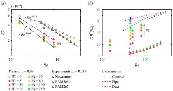
1. Introduction
It is well known that the addition of a small amount of long-chain flexible polymer leads to substantial drag reduction (DR) in wall-bound unidirectional turbulent shear flows. Since the discovery of this phenomenon by Toms (Reference Toms1949), it has become the subject of widespread research due to its fundamental and technological importance (see, e.g., the review by White & Mungal (Reference White and Mungal2008)). Among the more than 70 years of studies on polymer-induced DR, the feature that has attracted the most attention is the intriguing asymptotic behaviour of the DR effect, namely, the maximum drag reduction (MDR) originally proposed by Virk, Mickley & Smith (Reference Virk, Mickley and Smith1970). Specifically, in the dilute solution limit the extent of DR increases with polymer concentration and/or molecular weight and the commensurate elastic forces typically quantified by the Weissenberg number
 $Wi$
; however, this increase is eventually bounded by an upper limit, namely MDR, which is considered to depend solely on fluid inertia (quantified by Reynolds number,
 $Re$
) and to be insensitive to solvent and polymer properties (Xi Reference Xi2019). The mean velocity profile of the MDR state usually follows an empirical logarithmic law, that is, Virk’s asymptote (Virk et al. Reference Virk, Mickley and Smith1970). In addition, in the MDR state, the full polymer additives cannot eliminate turbulence, which poses the challenge of understanding the persistence of turbulence even at vanishingly small Reynolds stresses (Warholic, Massah & Hanratty Reference Warholic, Massah and Hanratty1999). To that end, since its discovery, the mechanistic understanding of the Virk’s asymptote that emerges from the complex interaction between small-scale turbulent vortices and microscale polymer dynamics has fascinated the community engaged in developing first-principal models and simulations that can faithfully predict the complex spatiotemporal dynamics of polymeric flows.
In the past three decades, the use of sophisticated experimental techniques and commensurate numerical simulations has led to a deeper mechanistic understanding of the aforementioned MDR state. Regarding the physical nature of this asymptotic flow state in planar shear turbulent flows (e.g. pipe and channel flows), two different points of view have gained significant traction (Xi Reference Xi2019; Dubief, Terrapon & Hof Reference Dubief, Terrapon and Hof2023). The first perspective views MDR as a marginal, ‘hibernating’ turbulent state, where the turbulent vortices are greatly suppressed and only a small population of small-scale hairpin vortices remains. This suggests that MDR is inherently a part of Newtonian turbulence, and it appears due to the introduced polymers (Xi & Graham Reference Xi and Graham2010, Reference Xi and Graham2012). Typically, the elastic torque produced by stretching polymers acts opposite to the rotation of small-scale vortices near the wall (Kim et al. Reference Kim, Li, Sureshkumar, Balachandar and Adrian2007, Reference Kim, Adrian, Balachandar and Sureshkumar2008), resulting in the weakening of vortical structures that give rise to Reynolds stresses (Li, Sureshkumar & Khomami Reference Li, Sureshkumar and Khomami2006; Teng et al. Reference Teng, Liu, Lu and Khomami2018) and significant flow intermittency (i.e. longer ‘hibernating’ periods) (Graham Reference Graham2014; Li, Sureshkumar & Khomami Reference Li, Sureshkumar and Khomami2015). Hence, the dynamics of suppressed vortices is closely related to the MDR dynamics. In the ‘hibernating state’, the intensity and number of small-scale turbulent vortices are too weak and too few to sufficiently stretch the polymers and generate significant polymer stress; therefore, the polymers cannot further suppress the turbulent flow motions (Xi Reference Xi2019; Zhu & Xi Reference Zhu and Xi2021).
The second viewpoint considers MDR to be a regime of elastoinertial turbulence (EIT) that is sustained by both inertial and elastic forces (Dubief et al. Reference Dubief, Terrapon and Hof2023) and is distinguished by small-scale spanwise cylindrical structures (Dubief, Terrapon & Soria Reference Dubief, Terrapon and Soria2013; Sid, Terrapon & Dubief Reference Sid, Terrapon and Dubief2018; Shekar et al. Reference Shekar, McMullen, Wang, McKeon and Graham2019). In this regard, MDR is a state disconnected from Newtonian (inertial) turbulence. This is supported by the observation that for turbulent pipe flows near the transition threshold, a continuous increase in polymer concentration leads to a reverse transition and subsequently to a relaminarization of turbulence, as well as the elimination of turbulent vortices (Choueiri, Lopez & Hof Reference Choueiri, Lopez and Hof2018; Lopez, Choueiri & Hof Reference Lopez, Choueiri and Hof2019). In this scenario, the drag exceeds the MDR limit and, in turn, reverts to the laminar value. Further enhancement of polymer elasticity triggers a secondary instability, leading to EIT, with the characteristic drag level of the MDR asymptote (Samanta et al. Reference Samanta, Dubief, Holzner, Schäfer, Morozov, Wagner and Hof2013). Small-scale spanwise cylindrical vortices have been found to play a crucial role in the self-sustaining process of EIT (Dubief et al. Reference Dubief, Terrapon and Soria2013; Zhang et al. Reference Zhang, Shao, Li, Ma, Zhang and Li2021a ). Specifically, the polymer body force induced by sheet-like high polymer extension creates these vortical structures, which in turn perturb the stress field of the polymer through the pressure redistribution effect (Terrapon, Dubief & Soria Reference Terrapon, Dubief and Soria2015). More recently, the two perspectives above are harmonized by Wang et al. (Reference Wang, Zhang, Wang, Li, Zhang and Li2023). By carefully examining the small-scale vortical structures and associated turbulence dynamics, these authors argue that maximum chain extensibility is the parameter of critical importance in determining the essence of MDR. This is consistent with previous studies by Khomami and colleagues (Li et al. Reference Li, Sureshkumar and Khomami2006, Reference Li, Sureshkumar and Khomami2015).
The studies above provide a summary of how macromolecules and small-scale vortices ‘dubbed’ shear energized vortices (SEVs) interact. Here, the term SEV refers to small-scale vortical structures sustained essentially by shear instabilities, and these vortices usually populate the wall region of planar shear turbulent flows, such as hairpin vortices and quasistreamwise vortices. Furthermore, the presence of system rotation or geometric curvature can induce the formation of additional small-scale turbulent vortices. The strong coupling between these additional small-scale vortices and polymer dynamics can lead to dramatically different asymptotic drag-limiting states (Zhu et al. Reference Zhu, Wan, Lin, Liu, Lu and Khomami2023; Lin et al. Reference Lin, Song, Liu, Wan, Lu and Khomami2024). For example, in addition to SEVs in wall-bounded turbulence, strong rotation in the spanwise-rotating plane Couette flow (RPCF) gives rise to additional small-scale Coriolis-force-generated turbulent vortices that are streamwise oriented and attached to the wall (Tsukahara, Tillmark & Alfredsson Reference Tsukahara, Tillmark and Alfredsson2010). These vortices can transport highly stretched polymer chains from the walls to the bulk, which in turn leads to incoherent transport of polymer stresses and results in notable drag enhancement (DE) (Zhu et al. Reference Zhu, Song, Lin, Liu, Lu and Khomami2022), leading to a novel maximum drag enhancement (MDE) state (Zhu et al. Reference Zhu, Wan, Lin, Liu, Lu and Khomami2023). To be more specific, Coriolis-force-generated vortices exhibit saturation of transverse momentum exchange with increased
 $Wi$
, leading to an asymptotic DE flow state. Another example of typical small-scale turbulent vortices is the centrifugal-force-induced G
 $\ddot {\text {o}}$
rtler vortices commonly seen in high-curvature (quantified by radius ratio
 $\eta =R_i/R_o=0.5$
, where
 $R_i$
and
 $R_o$
correspond to the inner and outer cylinder radii, respectively) Taylor–Couette flow (TCF) (Dong Reference Dong2007). Interestingly, by gradually increasing
 $Wi$
asymptotic MDE states appear in a wide-gap turbulent TCF in the Reynolds number range of
 $Re=1500\sim 8000$
(Lin et al. Reference Lin, Song, Liu, Wan, Lu and Khomami2024). In this case, the MDE state results from the creation and eventual saturation of small-scale elastic and inertioelastic G
 $\ddot {\text {o}}$
rtler vortices in the inner- and outer-wall regions (Liu & Khomami Reference Liu and Khomami2013), respectively. These vortical structures also facilitate efficient incoherent transport of polymer stress (Song et al. Reference Song, Teng, Liu, Ding, Lu and Khomami2019), resulting in a significant development of polymer stress. Despite the opposite polymer-induced drag modification (DM), the MDE and classical MDR flow states have important similarities. Here we would like to emphasize one of the most important similarities, namely, the drastic reduction in the Reynolds stresses up to
 $\sim 80\%$
(Samanta et al. Reference Samanta, Dubief, Holzner, Schäfer, Morozov, Wagner and Hof2013; Zhu et al. Reference Zhu, Wan, Lin, Liu, Lu and Khomami2023). In both cases, this reduction occurs because of the significant suppression of SEV by polymer additives. Hence, the MDE is a unique drag-limiting state with a Reynolds stress reduction similar to that of the MDR but with significant polymer-induced DE.
To date, most studies have focused on the drag-limiting states that arise from the interaction of polymer additives and small-scale turbulent vortices. However, in important canonical wall-bounded turbulent flows, such as plane and Taylor–Couette flows, large-scale structures (LSSs) have pronounced effects on the flow dynamics, including the self-sustaining process of turbulence and the wall scaling law (Orlandi, Bernardini & Pirozzoli Reference Orlandi, Bernardini and Pirozzoli2015; Rawat et al. Reference Rawat, Cossu, Hwang and Rincon2015). Here, LSSs refer to flow structures that span the gap, that is, they usually have a transverse length scale comparable to the gap width. In fact, recent studies have shown that intriguing phenomena arise in wall-bounded flows because of the interaction between polymers and LSSs. For example, the viscoelastic plane Couette flow exhibits DR when large-scale roll cells occupy the entire gap (Pereira et al. Reference Pereira, Mompean, Thais and Soares2017a
,Reference Pereira, Mompean, Thais, Soares and Thompson
b
). Compared with channel flow with only small-scale vortices, LSSs in plane Couette flow have a significant impact on energy exchange between polymers and turbulent motions (Teng et al. Reference Teng, Liu, Lu and Khomami2018). Another common type of LSSs is Taylor vortices in TCF. For moderate
 $\eta =0.72\sim 0.912$
, we found that polymer additives lead to a better organization of large-scale Taylor vortices, which in turn enhances the flow drag through stronger coherent angular momentum transport (Song et al. Reference Song, Teng, Liu, Ding, Lu and Khomami2019). Moreover, a very recent experimental study (Zhang et al. Reference Zhang, Fan, Su, Xi and Sun2025) has detected an asymptotic drag-reducing state in a wide-gap TCF with
 $\eta =0.714$
. It is found that at high curvature the effects of polymers on the large-scale Taylor vortices are only marginal. However, because of the lack of experimental techniques for characterizing polymer deformation and associated polymer stress, the underlying mechanisms associated with polymer dynamics is unknown. Although these studies provide preliminary information on the interaction between turbulent LSSs and polymers, a comprehensive investigation of the asymptotic property in this flow is still lacking. On the basis of the fact that turbulent vortices play a dual role in generating Reynolds stress and homogenizing polymer stress, there exists a potential to explore asymptotic flow states with different extents of DM. To that end, the following fundamental questions are raised. (i) Can polymers lead to asymptotic drag-limiting states (MDE or MDR) in turbulent wall-bounded flows containing LSSs (for example, low-curvature small-gap TCF)? (ii) Do novel turbulence and polymer dynamics exist in this asymptotic flow state? (iii) What is the mechanism by which LSSs influence the asymptotic drag-limiting state?
To answer these questions, we have chosen the low-curvature TCF geometry to minimize the influence of Görtler vortices, which allows a detailed examination of the interaction between the polymer chain dynamics and LSSs. To this end, we observe a novel polymer-induced MDR state in the turbulent Taylor vortex regime (
 $Re$
ranging from
 $1500$
to
 $8000$
), at different maximum chain extensibility (
 $L=50\sim 200$
) and a wide range of fluid elasticity (
 $Wi=0\sim 150$
). The dominant flow structure in this asymptotic drag-limiting flow state is the LSSs. To obtain a mechanistic understanding of the MDR in the TCF, we performed a systematic investigation of the turbulence and polymer chain dynamics. These detailed studies underscore the significant differences between the MDR flow state in TCF and channel/pipe flows. Finally, we elucidate the influence of maximum chain extensibility on dominant flow structures and the extent of DR in this asymptotic flow state.
2. Numerical details
2.1. Governing equations
We used direct numerical simulations (DNS) to investigate the flow dynamics of viscoelastic TCF with inner rotating and outer stationary cylinders. Similarly to our previous studies on drag-limiting behaviours of viscoelastic turbulent flows (Zhu et al. Reference Zhu, Wan, Lin, Liu, Lu and Khomami2023; Lin et al. Reference Lin, Song, Liu, Wan, Lu and Khomami2024), the constitutive equation FENE-P (finitely extensible nonlinear elastic-Peterlin) is adopted to model the polymeric contribution to total stress. We have chosen
 $d=R_{o}-R_{i}$
,
 $d/\Omega R_i$
,
 $\Omega R_{i}$
,
 $\rho (\Omega R_{i})^2$
and
 $\eta _{p} \Omega R_{i} /d$
as characteristic scales for length, time, velocity
 $\boldsymbol {u}$
, pressure
 $P$
and polymer stress
 $\boldsymbol {\tau }$
, respectively. Here,
 $\Omega$
denotes the angular velocity of the inner cylinder,
 $\rho$
represents the density of the fluid, and the total viscosity of the solution
 $\eta _t$
is the sum of the solvent contributions
 $(\eta _s)$
and the polymeric contributions
 $(\eta _p)$
. The resulting non-dimensional governing equations for incompressible, viscoelastic flow of FENE-P fluids are given as follows:
 \begin{align} {\boldsymbol {\nabla }}\,{\boldsymbol {\cdot }}\,\boldsymbol {u}& = 0,\end{align}
 \begin{align} \frac {\partial \boldsymbol {u}}{\partial t}+\boldsymbol {u}\,{\boldsymbol {\cdot }}\, {\boldsymbol {\nabla }} \boldsymbol {u}=-{\boldsymbol {\nabla }} P&+\frac {\beta }{Re}\nabla ^2\boldsymbol {u}+\frac {1-\beta }{Re}{\boldsymbol {\nabla }} \,{\boldsymbol {\cdot }}\, \boldsymbol {\tau }\end{align}
and
 \begin{equation} \frac {\partial \unicode{x1D63E}}{\partial t}+\boldsymbol {u}\,{\boldsymbol {\cdot }}\, {\boldsymbol {\nabla }} \unicode{x1D63E}=\unicode{x1D63E}\,{\boldsymbol {\cdot }}\, {\boldsymbol {\nabla }} \boldsymbol {u}+\left ( {\boldsymbol {\nabla }} \boldsymbol {u} \right )^{T}{\boldsymbol{\cdot}}\, {\unicode{x1D63E}}-\boldsymbol {\tau }, \end{equation}
where
 $\unicode{x1D63E}$
is the symmetric positive definite conformation tensor that represents the ensemble average of the second moment of the end-to-end vector of the polymer chain. The parameter
 $\beta =\eta _s/\eta _t$
is the solvent to total zero-shear viscosity ratio and
 $Re=\rho \Omega R_i d/\eta _t$
is the Reynolds number based on the inner cylinder velocity. Furthermore, to obtain a closed-form constitutive equation for the polymer stress, the following relationship is adopted in the FENE-P model:
 \begin{equation} \boldsymbol {\tau }=\frac {f(\unicode{x1D63E}\kern1.5pt)\unicode{x1D63E}-\unicode{x1D644}}{Wi}, \end{equation}
where
 $f(\unicode{x1D63E}\kern1.5pt)=(L^2-3)/[L^2-\textrm {trace}(\unicode{x1D63E}\kern1.5pt)]$
is the Peterlin function and
 $L$
denotes the maximum chain extensibility. The parameter
 $Wi=\lambda R_i \Omega /d$
is the Weissenberg number with
 $\lambda$
being the relaxation time of the polymer solutions.
Boundary conditions are supplemented to solve these equations. That is, the axial direction is assumed to be periodic, whereas the cylinder walls are subjected to non-slip and non-penetration boundary conditions. It should also be noted that no boundary conditions are imposed on the walls of
 $\unicode{x1D63E}$
since the evolution equation for the conformation tensor is hyperbolic.
2.2. Numerical methods and computational settings
In this study, we employ an in-house finite-difference algorithm (Lin et al. Reference Lin, Wan, Zhu, Liu, Lu and Khomami2022) to perform DNS to solve the governing equations (2.1)–(2.4). Specifically, for temporal integration we use a combination of a fractional-step third-order low-storage Runge–Kutta method and the Crank–Nicolson scheme for the viscous terms. In particular, in the constitutive equation (2.3) the stress relaxation term is implicitly advanced to enforce the boundedness of the polymer conformation tensor (Somasi et al. Reference Somasi, Khomami, Woo, Hur and Shaqfeh2002; Dubief et al. Reference Dubief, Terrapon, White, Shaqfeh, Moin and Lele2005; Song et al. Reference Song, Lin, Liu, Lu and Khomami2021a
). We employ a combination of a staggered grid arrangement and a well-established central second-order accurate finite-difference scheme (Verzicco & Orlandi Reference Verzicco and Orlandi1996) for spatial discretization. This technique is routinely used in simulations of turbulent TCF (Ostilla-Mónico et al. Reference Ostilla-Mónico, Stevens, Grossmann, Verzicco and Lohse2013, Reference Ostilla-Mónico, van der Poel, Verzicco, Grossmann and Lohse2014b
) due to its inherent discrete energy conservation property (Moin & Verzicco Reference Moin and Verzicco2016). However, the treatment of the convection term in the constitutive equation (2.3) requires special consideration due to the hyperbolic nature of (2.3) at high
 $Wi$
, which could lead to significant numerical instability (Talwar, Ganpule & Khomami Reference Talwar, Ganpule and Khomami1994; Yang & Khomami Reference Yang and Khomami1999; Alves, Oliveira & Pinho Reference Alves, Oliveira and Pinho2021). To that end, we adopt the Kurganov–Tadmor shock capture scheme (Vaithianathan et al. Reference Vaithianathan, Robert, Brasseur and Collins2006) to accurately resolve the sharp gradients in the polymer stress field. This scheme maintains the symmetric positive definite property of
 $\unicode{x1D63E}$
during time integration with an appropriately small time step, by monitoring the eigenvalues of the conformation tensor for all grid points in our present simulations. Furthermore, we use uniform grid spacing in the axial and azimuthal directions, while in the radial direction a clipped Chebyshev-type clustering is implemented near both walls to increase the near-wall grid resolution required for simulations of wall-bounded turbulence. In general, our solver is an efficient and high-fidelity algorithm for large-scale DNS over a wide range of elastically modified turbulent flow regimes, see Lin et al. (Reference Lin, Wan, Zhu, Liu, Lu and Khomami2022) for additional details.
To achieve the desired flow field, that is, one that contains small-scale SEVs, large-scale Taylor vortices and devoid of Görtler vortices, we perform simulations in a low-curvature small-gap viscoelastic TCF at a radius ratio of
 $\eta =R_i/R_o=0.99$
. This allows a clear comparison with the MDE asymptote in the high-curvature (
 $\eta =0.5$
) TCF (Lin et al. Reference Lin, Song, Liu, Wan, Lu and Khomami2024), where the dominant flow structure is that of small-scale Görtler vortices. Furthermore, we have chosen
 $\beta = 0.9$
to mimic dilute polymeric solutions with negligible shear-thinning of viscosity. To gain a comprehensive picture of flow transitions in the route to flow states exhibiting asymptotic drag behaviour, we perform extensive DNS in
 $L=100$
over a wide range of
 $Wi=0\sim 150$
in
 $Re$
of
 $1500, 5000$
and
 $8000$
. Recent studies have shown that varying the maximum extensibility of the polymer chain leads to significant qualitative flow changes (Song et al. Reference Song, Wan, Liu, Lu and Khomami2021b
; Wang et al. Reference Wang, Zhang, Wang, Li, Zhang and Li2023; Beneitez et al. Reference Beneitez, Page, Dubief and Kerswell2024). To this end, we have also performed simulations with
 $L=50$
and
 $L=200$
at
 $Re=5000$
to determine the influence of the maximum chain extensibility on flow dynamics and the extent of drag. Table 1 contains the simulation parameters. It is also worth mentioning that for the selected low-curvature geometry, the TCF tends to approach its limiting case, that is, the curvature-free RPCF, in which intriguing polymer-induced DM has also been observed (Zhu et al. Reference Zhu, Song, Lin, Liu, Lu and Khomami2022, Reference Zhu, Wan, Lin, Liu, Lu and Khomami2023). According to Brauckmann, Salewski & Eckhardt (Reference Brauckmann, Salewski and Eckhardt2016), the TCFs in
 $Re=1500,5000$
and
 $8000$
with
 $\eta =0.99$
are related to the RPCF systems in sequence with
 $Re_s = 1507.5, 5025.1$
and
 $8040.2$
with weak rotation
 $R_{\Omega }=0.01$
, where
 $Re_s$
is the shear Reynolds number and
 $R_{\Omega }$
is the rotation number in the RPCF.
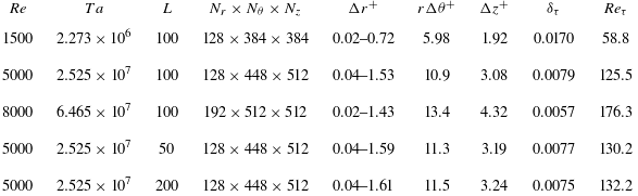
Numerical parameters and grid resolutions at
 $Wi=150$
for various
 $Re$
and
 $L$
. The superscript ‘
 $+$
’ denotes the quantities non-dimensionalized by the viscous length scale
 $\delta _\tau =\eta _t/\rho /u_\tau$
; the friction velocity is defined as
 $u_\tau =\sqrt {\tau _w/\rho }$
, where
 $\tau _w$
is the total wall stress (the sum of viscous stress and polymer stress); the friction Reynolds number is defined as
 $Re_\tau =\rho u_\tau d/\eta _t$
. For each
 $Re$
, we have also provided the corresponding Taylor number (
 $Ta$
), which is defined as
 $Ta = [(1+\eta )^4(R_o - R_i)^2(R_o + R_i)^2(\Omega -\Omega _o)^2]/(64\eta ^2 \nu ^2)$
, with
 $\Omega _o$
being the angular velocity of the outer cylinder (
 $\Omega _o=0$
in our cases) (Grossmann et al. Reference Grossmann, Lohse and Sun2016). Also, the kinematic viscosity is denoted as
 $\nu$
.

In the numerical simulation of TCF, the length of the axial computational domain (
 $L_z$
) is a critical parameter, as it determines the axial length scale of the LSS. Based on extensive a priori test calculations,
 $L_z$
is set as
 $4\pi$
so that it contains at least two pairs of large-scale Taylor vortices in the asymptotic drag-limiting states. In addition, one must ensure that
 $L_z=4\pi$
is long enough to allow an accurate capture of the axial motions of LSSs, as demonstrated by the DNS of transitional viscoelastic TCF that involves vortex merging and splitting events (Lopez Reference Lopez2022). To reduce computational requirements for small-gap geometry (large radius ratio) (Ostilla-Mónico et al. Reference Ostilla-Mónico, Huisman, Jannink, Van Gils, Verzicco, Grossmann, Sun and Lohse2014a
,Reference Ostilla-Mónico, van der Poel, Verzicco, Grossmann and Lohse
b
, Reference Ostilla-Mónico, Verzicco and Lohse2015; Brauckmann et al. Reference Brauckmann, Salewski and Eckhardt2016), we chose azimuthal periodicity
 $n_{sym}=16$
to reduce the natural azimuthal length to
 $L_{\theta }=2\pi R_a /n_{sym}=39.1$
with the mean radius
 $R_a=(R_i+R_o)/2$
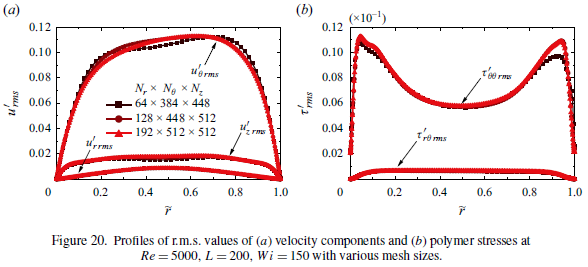
. To that end, in Appendix A we have verified that the chosen computational domain faithfully captures the flow structures of interest. Table 1 contains the grid size and associated spatial resolutions (in units of inner wall) in the drag-limiting states in viscoelastic TCF. Evidently, the results reported based on the grid sizes listed in table 1 are accurate (see extensive grid convergence studies reported in Appendix B). The simulation protocol is as follows. We first obtain the Newtonian turbulent flow field at each
 $Re$
and start all other simulations at a new
 $Wi$
from the chaotic flow states obtained at the previous lower
 $Wi$
. Simulations are performed with a small time step of
 $\unicode{x0394} t=0.005$
and sufficiently long calculations of
 $O (1000T)$
, where
 $T=d/(R_i\Omega )$
is the convective time unit, to ensure that we obtain statistically stationary flows. In addition, an ensemble average is performed over a time period of at least 1000
 $T$
to obtain reliable turbulence statistics.
3. Characterization of novel MDR state
In this section, we discuss the drag-limiting behaviour of viscoelastic TCF with different
 $Re$
, with particular emphasis on realization of the MDR state. Similarly to our previous studies on the DM in TCF of dilute polymeric solutions (Song et al. Reference Song, Teng, Liu, Ding, Lu and Khomami2019; Lin et al. Reference Lin, Song, Liu, Wan, Lu and Khomami2024), we use the Nusselt number (
 $Nu_{\omega }=J^{\omega }/J^{\omega }_{lam}$
) which represents the overall transport of angular momentum to quantify drag (Eckhardt, Grossmann & Lohse Reference Eckhardt, Grossmann and Lohse2007). Specifically,
 $J^{\omega }$
is a conserved quantity that characterizes the radial current of angular momentum flux,
 \begin{equation} J^{\omega }=r^3\left [ \left \lt u_r\omega \right \gt -\frac {\beta }{Re}\frac {\partial \left \lt \omega \right \gt }{\partial r}-\frac {\left ( 1-\beta \right )}{Re}\frac {\left \lt \tau _{r\theta } \right \gt }{r} \right ], \end{equation}
where
 $\omega =u_{\theta }/r$
is the angular velocity, and
 $\langle \cdot \rangle =\langle \cdot \rangle _{\theta ,z,t}$
denotes hereafter the averaging of the ensemble in the
 $\theta -$
and
 $z-$
directions and in time. This allows for the evaluation of the fluctuating part of the variable
 $\phi$
as
 $\phi '=\phi -\left \langle \phi \right \rangle$
. It should be noted that although
 $r^3$
appears in (3.1),
 $J^{\omega }$
is a quantity independent of
 $r$
, which represents the conserved transverse current of azimuthal motion, transporting
 $\omega$
in the radial direction. In addition,
 $J^{\omega }_{lam}=2(\omega _i-\omega _o)r_{i}^{2}r_{o}^{2}/Re(r_{o}^{2}-r_{i}^{2})$
corresponds to the Newtonian non-vortical laminar current, which is induced solely by molecular diffusion. Hence, we compute the extent of DR as
 $(Nu_{\omega }-Nu_{\omega }^{N})/Nu_{\omega }^{N}$
with
 $Nu_{\omega }^{N}$
being the Newtonian value at the corresponding
 $Re$
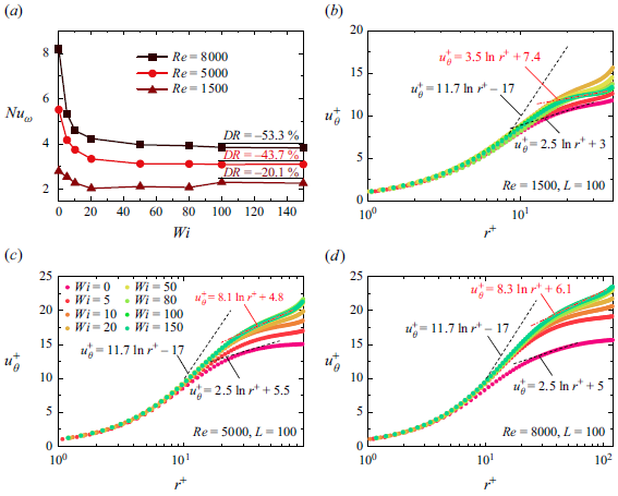
. As depicted in figure 1(
 $a$
), for the low
 $Wi$
regime (
 $Wi\leqslant 20$
), DR is continuously enhanced. That is, as the elastic effects grow larger,
 $Nu_{\omega }$
continues to decrease with increasing
 $Wi$
at all
 $Re$
. This phenomenon is remarkably similar to the polymer-induced DR in planar shear channel/pipe flows because, in both cases, polymer elasticity suppresses SEVs. Hence, when
 $Nu_{\omega }$
plateaus at sufficiently high
 $Wi$
, we attain the MDR states. Specifically,
 $Nu_{\omega }$
shows no visible changes to the naked eye for
 $Wi\geqslant 50$
at
 $Re=5000, 8000$
and for
 $Wi\geqslant 100$
at
 $Re=1500$
. The extents of DR in these asymptotes are
 $-20.1\, \%$
,
 $-43.7\, \%$
and
 $-53.3\, \%$
for
 $Re=1500$
, 5000 and 8000, respectively. Hence, the extent of DR has a monotonic dependence on
 $Re$
. This is consistent with experimental observations in drag-reducing channel/pipe flows (Virk Reference Virk1975; Xi Reference Xi2019). Furthermore, the DR rate realized in this study is higher than that (
 $\sim -20\, \%$
) obtained by recent experiments for TCF at
 $\eta =0.714$
(Zhang et al. Reference Zhang, Fan, Su, Xi and Sun2025). However, at
 $Re$
= 8000 (
 $Re_{\tau }=258$
) the level of DR is still relatively lower compared with the classical MRD state realized in channel flow (Li et al. Reference Li, Sureshkumar and Khomami2006; Dallas, Vassilicos & Hewitt Reference Dallas, Vassilicos and Hewitt2010) (for example,
 $-74.0\, \%$
DR at
 $Re_{\tau }=180$
), which is clearly demonstrated in Appendix D. This clearly shows that the MDR states realized in TCF do not follow the well-known Virk limit, indicating that these asymptotic drag-limiting states are distinct from those in planar shear turbulent flows. This deviation is expected because, as shown below, the MDR states in TCF are in different flow regimes that contain LSSs.
(
 $a$
) Nusselt number
 $Nu_{\omega }$
versus
 $Wi$
at various
 $Re$
with
 $L=100$
. The extent of DR for the highest
 $Wi=150$
realized in our simulations is reported. The log plots of mean velocity profile
 $u_{\theta }^{+}$
in the inner-half of the gap versus wall-normal distance
 $r^+$
for (
 $b$
)
 $Re=1500$
, (
 $c$
)
 $Re=5000$
and (
 $d$
)
 $Re=8000$
. Here,
 $u_{\theta }^{+}$
is calculated as
 $(1-\langle u_{\theta }\rangle )/u_\tau$
. The log law plot of
 $u_{\theta }^{+}=\kappa \textrm {ln}(r^+)+C$
is added hereafter as a visual guide, with
 $\kappa =2.5$
and
 $11.7$
corresponding to the von Kármán law and the Virk law, respectively.

To identify MDR asymptotes in viscoelastic TCF at different
 $Re$
, we have also used dimensionless mean velocity profiles based on traditional inner variable scaling. For ease of comparison, we have added the Virk law of the classical MDR in planar shear flows (Virk Reference Virk1975) to these plots. As shown in figure 1(
 $b$
,
 $c$
), similar to other polymer drag-reducing flows, the increase in
 $Wi$
in the range of
 $5- 20$
leads to a gradual increase in
 $u_{\theta }^{+}$
in the core region. As elastic effects are further enhanced (
 $Wi\geqslant$
50), a continuous increase is observed for
 $Re=5000, 8000$
(see figure 1
c,d), while the velocity decreases in the core region for
 $Re=1500$
(see figure 1
 $b$
), corresponding to the slight increase of
 $Nu_{\omega }$
shown in figure 1(
 $a$
). However, the
 $u_{\theta }^{+}$
profiles for all
 $Re$
considered show an asymptotic limit at sufficiently large
 $Wi$
, that is, they collapse onto a single curve. Hence, we attain asymptotic flow states although the mean velocity profiles lie below Virk’s asymptote. As expected, this depiction also supports the idea that polymer-induced asymptotic behaviours also exist in low-curvature small-gap TCF while the resulting flow states may differ from the classical MDR state of viscoelastic turbulent channel and pipe flows. This is rationale because the classical MDR states are realized in the flow regime dominated by small-scale SEVs. Hence, the deviation from the Virk MDR velocity profile is also observed in the experiments for asymptotic DR states of TCF with
 $Re$
up to
 $2.5\times 10^4$
, which are still dominated by turbulent Taylor vortices (Zhang et al. Reference Zhang, Fan, Su, Xi and Sun2025). In addition, it is worth comparing the current MDR state with the MDE state in high-curvature (
 $\eta =0.5$
) TCF (Lin et al. Reference Lin, Song, Liu, Wan, Lu and Khomami2024), in which the mean velocity profile closely follows a logarithmic-like law with an identical slope. By fitting the
 $u_{\theta }^{+}$
profiles in the regions
 $r^+\geqslant 20$
for
 $Re=1500$
and
 $r^+\geqslant 30$
for
 $Re=5000, 8000$
, we do not find a unified logarithmic-like law in the parameter range considered in the present study. These discrepancies point to the fact that MDR in TCF is a novel asymptotic flow state, as revealed by the distinct flow structures discussed below.
To elucidate the flow transitions that lead to the realization of the MDR flow state in viscoelastic TCF, we examine the evolution of space–time plots of radial velocity
 $u_r$
enroute to MDR. This also allows for highlighting the differences in flow structures between MDR in TCF and in channel/pipe flows. As shown in figure 2(
 $a$
), inflow (blue) and outflow (red) streaks that are highly oscillatory in time signify typical turbulent Taylor vortices (Andereck, Liu & Swinney Reference Andereck, Liu and Swinney1986; Grossmann, Lohse & Sun Reference Grossmann, Lohse and Sun2016). Upon the introduction of polymers, the suppression effect of elasticity is observed by weaker oscillations of streaks, as well as fewer inflow (outflow) spots in the flow field (see figure 2
 $b$
–
 $d$
). The change in the number of Taylor vortices, i.e. from four to five pairs, gives rise to the slight increase in flow drag from
 $Wi=80$
to 100 (see figure 1
 $a$
). This is consistent with the experimental observation that the torque in the flow state with a larger number of Taylor rolls is higher at low
 $Re$
(Martínez-Arias et al. Reference Martínez-Arias, Peixinho, Crumeyrolle and Mutabazi2014). Eventually, identical flow patterns at
 $Wi=100, 150$
(see figure 2
 $e$
,
 $f$
) signify the existence of an asymptotic flow state. Interestingly, achieving the MDR state at
 $Re=1500$
reveals a reverse transition route from turbulent Taylor vortices to a flow pattern similar to wavy turbulent vortices (Dutcher & Muller Reference Dutcher and Muller2009). Specifically, in this wavy-turbulent-vortices-like flow state, the large-scale Taylor vortices are wavy. Meanwhile, the velocity streaks shown as cutoffs in the space–time plots (see the blue frames marked in figure 2
 $e$
,
 $f$
) provide visual evidence of the strong intermittency in the velocity streaks. It should be noted that at low
 $Re$
the existence of the reverse transition and secondary instability leading to EIT in channel and pipe flows when approaching the MDR state is well documented (Choueiri et al. Reference Choueiri, Lopez and Hof2018; Shekar et al. Reference Shekar, McMullen, Wang, McKeon and Graham2019; Lopez et al. Reference Lopez, Choueiri and Hof2019). However, here we do not obtain a non-vortical fully laminar state enroute to MDR in TCF. This could be due to: (i)
 $Re=1500$
being still high in TCF; (ii) despite the low curvature at
 $\eta =0.99$
, the hoop stress rendered by the curved streamline persists to destabilize the flow. Nevertheless, based on the examination of flow structures at
 $Re=1500$
, we postulate that LSSs are the dominant flow feature in this novel MDR flow state.
Space–time plots of radial velocity
 $u_r$
along axial sampling line at the middle of the gap (
 $\tilde {r}=0.5$
) for (
 $a$
)
 $Wi=0$
, (
 $b$
)
 $Wi=5$
, (
 $c$
)
 $Wi=20$
, (
 $d$
)
 $Wi=50$
, (
 $e$
)
 $Wi=100$
and (
 $f$
)
 $Wi=150$
at
 $Re=1500$
. Hereafter
 $\tilde {r}=(r-R_i)/d$
represents the dimensionless distance to the inner cylinder wall. The blue dashed frames indicate the time period when strong intermittency occurs.

Although LSSs are the dominant flow feature in MDR at
 $Re=1500$
, the dominance of large-scale flow structures at MDR at higher
 $Re$
needs to be closely examined. To that end, we examined the evolution of the space–time plots at
 $Re=5000$
and
 $8000$
(see figures 3 and 4). We observe a similar phenomenon in the low
 $Wi$
regime (
 $Wi\lt 20$
). That is, as one approaches the MDR state, we observe suppression of small-scale motions and stabilization of large-scale Taylor vortices (figures 3
 $b$
and 4
 $b$
). In addition, the identical flow patterns at
 $Wi\geqslant 50$
, consistent with the plateaus
 $Nu_{\omega }$
seen in figure 1(
 $a$
), are indicative of an asymptotic flow state. However, with high fluid inertia, LSSs cannot maintain a well-organized pattern as observed at
 $Re=1500$
. Specifically, the highly meandering inflow/outflow streaks in the axial space–time plots depict significant axial motions of these structures. Despite the random appearance of axial motions, the imprints of LSSs can still be observed, as marked by blue dashed lines in figures 3(
 $f$
) and 4(
 $f$
). This feature is also different from the MDE in high-curvature TCF (Lin et al. Reference Lin, Song, Liu, Wan, Lu and Khomami2024), where strong hoop stresses break down LSSs into small-scale elastic and inertioelastic Görtler vortices. Moreover, for TCF with different
 $\eta$
(
 $=0.714$
), it is found that the wavelength and pattern of LSSs are not changed in the asymptotic DR states (Zhang et al. Reference Zhang, Fan, Su, Xi and Sun2025). This is mainly attributed to the fact that for
 $\eta =0.714$
the strength of the LSSs has been enhanced by the stronger curvature (centrifugal) effects.
Space–time plots of radial velocity
 $u_r$
along axial sampling line at the middle of the gap (
 $\tilde {r}=0.5$
) for (
 $a$
)
 $Wi=0$
, (
 $b$
)
 $Wi=5$
, (
 $c$
)
 $Wi=20$
, (
 $d$
)
 $Wi=50$
, (
 $e$
)
 $Wi=100$
and (
 $f$
)
 $Wi=150$
at
 $Re=5000$
. The blue dashed lines indicate the outflow streaks associated with LSSs.

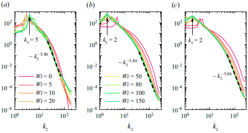
The power spectral density is used to quantify the persistence of LSSs in the MDR states. Specifically, we plot the one-dimensional spanwise spectra of the turbulent kinetic energy (TKE) in the
 $Re$
range considered in figure 5. Overall, all spectral curves show approximately eight orders of magnitude of energy decay, indicating that we have accurately captured the relevant spatial scales. The LSSs can be identified by the highest spectral peaks in the low-wavenumber range. Specifically, in the MDR regime, consistent with the flow structures illustrated by the space–time plots, we observe dominant spatial modes with wavenumbers
 $k_z=5, 2$
and 2 for
 $Re=1500$
,
 $5000$
and
 $8000$
, respectively. On the other hand, the energy transfer induced by small-scale motions is suggested by the spectral behaviour for the wavenumbers in the dissipation range. Interestingly, spectra show approximately
 $k_z^{-5.86}$
scaling at all
 $Re$
. This exponent value of the decaying law is slightly lower than the
 $-14/3$
law commonly seen in the classical MDR states of planar shear turbulent flows (Dubief et al. Reference Dubief, Terrapon and Soria2013; Wang et al. Reference Wang, Zhang, Wang, Li, Zhang and Li2023), indicating that small-scale motions present faster energy transfer for MDR states in low-curvature TCF.
Space–time plots of radial velocity
 $u_r$
along axial sampling line at the middle of the gap (
 $\tilde {r}=0.5$
) for (
 $a$
)
 $Wi=0$
, (
 $b$
)
 $Wi=5$
, (
 $c$
)
 $Wi=20$
, (
 $d$
)
 $Wi=50$
, (
 $e$
)
 $Wi=100$
and (
 $f$
)
 $Wi=150$
at
 $Re=8000$
. The blue dashed lines indicate the outflow streaks associated with LSSs.

One-dimensional spanwise spectra of the turbulent kinetic energy
 $(\langle \boldsymbol {u}' \cdot \boldsymbol {u}' \rangle /2)$
sampled at the middle of the gap for (
 $a$
)
 $Re=1500$
, (
 $b$
)
 $Re=5000$
and (
 $c$
)
 $Re=8000$
at various
 $Wi$
. The dominant spatial mode that has the highest energy at the MDR state is marked with black arrow. The decaying exponent
 $-5.86$
is obtained by fitting the spectral curve at
 $Re=8000, Wi=150$
in the region
 $k_z \geqslant 50$
.

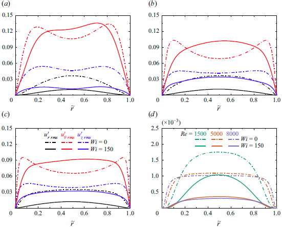
Profiles of the root-mean-square (r.m.s.) values of the velocity fluctuations for (
 $a$
)
 $Re=1500$
, (
 $b$
)
 $Re=5000$
and (
 $c$
)
 $Re=8000$
. (
 $d$
) Comparison of the Reynolds stress in Newtonian TCF and the MDR states for various
 $Re$
.

Overall, the above analyses have conclusively demonstrated the existence of a novel MDR state in viscoelastic TCF. This drag-limiting state is unique because of the persistence of LSSs in the flow field, which is distinct from other reported asymptotic flow states. Specifically, the dominant flow structures in MDR of channel/pipe flows are found to be small-scale (marginal inertial) streamwise or (elastoinertial) spanwise vortices (Dubief et al. Reference Dubief, Terrapon and Hof2023; Wang et al. Reference Wang, Zhang, Wang, Li, Zhang and Li2023), while in the MDE of RPCF and high-curvature TCF are small-scale Coriolis-force-generated vortices and elastic/inertioelastic Görtler vortices (Zhu et al. Reference Zhu, Wan, Lin, Liu, Lu and Khomami2023; Lin et al. Reference Lin, Song, Liu, Wan, Lu and Khomami2024), respectively. Thus, the flow dynamics associated with LSSs plays a critical role in maintaining this novel MDR flow state.
4. Turbulence dynamics in the MDR state
In what follows, we discuss the turbulence dynamics in the MDR states of TCF, with a particular focus on important flow characteristics that arise due to LSSs. It is well-known that the turbulent motions of vortical structures can generate Reynolds stresses. On the other hand, the interaction between polymers and vortical structures leads to the creation and homogenization of polymer stresses. To that end, we depict the dynamical changes of turbulent motions, namely, turbulent intensities and Reynolds stresses enroute to the MDR state in figure 6. Specifically, the peak values in the r.m.s. of azimuthal velocity fluctuations
 $u'_{\theta \ rms}$
indicate the presence of small-scale SEVs in the near-wall regions for Newtonian (
 $Wi=0$
) flows. Meanwhile, the peak values in
 $u'_{r \ rms}$
and
 $u'_{z \ rms}$
correspond to intense radial and axial fluctuation motions induced by large-scale Taylor vortices (Bilson & Bremhorst Reference Bilson and Bremhorst2007). In the MDR state (
 $Wi=150$
), we observe a redistribution of
 $u'_{\theta \ rms}$
as well as a reduction of
 $u'_{r \ rms}$
and
 $u'_{z \ rms}$
(see figure 6
 $a$
–
 $c$
). To that end, the two near-wall peaks in
 $u'_{\theta \ rms}$
have disappeared, while the values of the bulk region have become larger. This is a clear manifestation of the polymer-induced suppression of SEVs. Both
 $u'_{r \ rms}$
and
 $u'_{z \ rms}$
depict a significant reduction in value compared with their Newtonian counterpart, while their peaks are more pronounced in the middle of the gap (except for
 $Re=1500$
, in which
 $u'_{z \ rms}$
maintains its two near-wall peaks due to the well-organized LSSs). Changes in radial and axial turbulence intensities support the weakening of LSSs, which is manifested by (i) elastic stabilization, especially for
 $Re=1500$
(figure 2), and (ii) reduction in number, that is, from five pairs to two pairs for
 $Re=5000, 8000$
(figures 3 and 4). To that end, we observe distinct flow structures in the MDR state of TCF, as highlighted in figure 7. That is, polymers lead to a great suppression of SEVs, as indicated by the few remaining small-scale structures; while the LSSs persist in the asymptotic drag-limiting states, as evidenced by the long streamwise rolls. Eventually, owing to the above structural changes, we observe a significant reduction of Reynolds stresses (see figure 6
 $d$
), and a commensurate reduction of turbulent drag. Although the reduction of Reynolds stresses is a hallmark of drag-reducing flows, here, because of the presence of LSSs, the distribution of Reynolds stresses is dramatically different from the classical MDR state. Specifically, the peak value of Reynolds stresses occurs in the middle of the gap, while in the MDR state of channel/pipe flows it occurs in the near-wall regions where the SEVs are highly energetic (Dallas et al. Reference Dallas, Vassilicos and Hewitt2010; Wang et al. Reference Wang, Zhang, Wang, Li, Zhang and Li2023). Moreover, Reynolds stresses are commonly vanishingly small for MDR channel/pipe flows compared with Newtonian cases (Warholic et al. Reference Warholic, Massah and Hanratty1999; Choueiri et al. Reference Choueiri, Lopez and Hof2018). However, for TCF, they are comparable to their Newtonian counterparts due to the presence of LSSs (Zhang et al. Reference Zhang, Fan, Su, Xi and Sun2025), especially for
 $Re=1500$
.
Instantaneous flow structures visualized by the fluctuating streamwise velocity with
 $u_{\theta }'=\pm 0.1$
and coloured by the fluctuating radial velocity
 $u_r'$
for (
 $a$
) a typical Newtonian turbulence at
 $Re=1500$
and MDR states (
 $Wi=150$
) at (
 $b$
)
 $Re=1500$
, (
 $c$
)
 $Re=5000$
and (
 $d$
)
 $Re=8000$
.

In addition to Reynolds stress, polymer stress in viscoelastic wall-bounded turbulence also contributes to flow drag (see (3.1)). To that end, the development of polymer stress competes with the reduction of Reynolds stress, offsetting part of the DR effect. For example, in MDE states, significant polymer stress can even far exceed the suppressed Reynolds stress, resulting in remarkable DE (Zhu et al. Reference Zhu, Wan, Lin, Liu, Lu and Khomami2023; Lin et al. Reference Lin, Song, Liu, Wan, Lu and Khomami2024). Hence, the behaviour of polymer stress is closely related to the degree of DR that can be achieved in asymptotic flow states. To examine these intriguing polymer dynamics, we examine the
 $r\theta$
-component polymer stress that is directly related to flow drag. As depicted in figure 8(
 $a$
), for all MDR states under different
 $Re$
, the distribution of polymer stress is similar, i.e. the rescaled
 $\langle \tau _{r\theta } \rangle$
achieves a local maximum in the bulk bridging the two near-wall local minima. Increasing fluid inertia leads to a reduction in the magnitude of polymer stress, facilitating a higher DR rate in the MDR state with higher
 $Re$
.
In order to quantify the polymer stress in more detail,
 $\langle \tau _{r\theta } \rangle$
is decomposed into
 $\tau _{r\theta }^{e1}$
, which is induced by non-vortical flows and
 $\tau _{r\theta }^{e2}$
that arises due to interaction with vortical structures. Following Zhang et al. (Reference Zhang, Zhang, Li, Yu and Li2021b
) and Wang et al. (Reference Wang, Zhang, Wang, Li, Zhang and Li2023), we obtain
 $\tau _{r\theta }^{e1}$
by solving the FENE-P conformation tensor
 $\unicode{x1D63E}^{\kern1pt e1}$
in a non-vortical Couette flow as
 \begin{equation} \unicode{x1D63E}^{\kern1pt e1}=\left [ \begin{matrix} \frac {1}{f\left ( \unicode{x1D63E} \kern1.5pt \right )}& \frac {-Wi\cdot S}{f^2\left ( \unicode{x1D63E} \kern1.5pt \right )}& 0\\ \frac {-Wi\cdot S}{f^2\left ( \unicode{x1D63E} \kern1.5pt \right )}& \frac {L^2-\left ( L^2-1 \right )}{f\left ( \unicode{x1D63E} \kern1.5pt \right )}& 0\\ 0& 0& \frac {1}{f\left ( \unicode{x1D63E} \kern1.5pt \right )}\\ \end{matrix} \right ], \end{equation}
where
 $S=r ({\partial \langle u_{\theta }/r\rangle })/{\partial r}$
is the local shear rate of the mean flow. Therefore,
 $\tau _{r\theta }^{e2} = \langle \tau _{r\theta } \rangle - \tau _{r\theta }^{e1}$
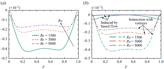
, represents the polymer stress generated by the interaction between polymers and vortical structures. Figure 8(
 $b$
) depicts the decomposed polymer stress in MDR states as a function of
 $Re$
. Interestingly, in a flow driven by wall motion (shear), the polymeric shear stress
 $\tau _{r\theta }^{e1}$
is quite small in magnitude. Hence, the vast majority of polymer stress comes from the contribution of
 $\tau _{r\theta }^{e2}$
, indicating the significant effect of vortical structures on polymer deformation. However, in low-curvature turbulent TCF LSSs coexist with SEVs. Hence, with this approach, one cannot unequivocally determine which vortical structures play the dominant role in the deformation of polymer chains. However, the more pronounced
 $\tau _{r\theta }^{e2}$
observed in MDR with
 $Re=1500$
is the basis for the fact that a well-organized LSS results in stronger polymer deformations and stresses.
(
 $a$
) Rescaled polymer stresses
 $(1-\beta )\langle \tau _{r\theta } \rangle /Re$
at the MDR state (
 $Wi=150$
) for various
 $Re$
. (
 $b$
) Decomposition of polymer stress into
 $\tau _{r\theta }^{e1}$
that induced by the non-vortical based flow and
 $\tau _{r\theta }^{e2}$
that interacts with vortical structures.

To further quantify the relationship between vortical structures and polymer dynamics and stresses, we performed POD analysis of the MDR states in TCF. The POD provides a global decomposition of field quantities into an orthonormal basis ordered in an optimal way to best represent the Euclidean norm (Lumley Reference Lumley1970). In turbulent flows, POD allows for the identification of dominant coherent structures (Taira et al. Reference Taira, Brunton, Dawson, Rowley, Colonius, McKeon, Schmidt, Gordeyev, Theofilis and Ukeiley2017). Furthermore, Wang et al. (Reference Wang, Graham, Hahn and Xi2014) extended this approach to the viscoelastic turbulent channel flow to examine the spatial structure of the dominant energetic component, assuming that
 $\textrm {trace}(\unicode{x1D63E}\kern1.5pt)$
is proportional to the elastic energy. To that end, we apply POD to fluctuating velocities and
 $\textrm {trace}(\unicode{x1D63E}\kern1.5pt)$
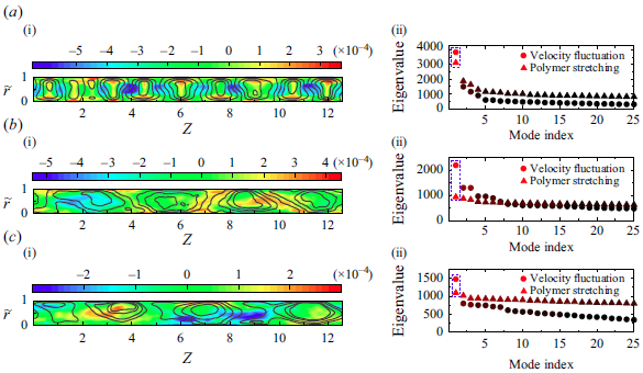
, to find the most energetic spatial modes, in terms of TKE and elastic energy. The leading mode is more obvious for the MDR state at
 $Re=1500$
(see figure 9
a ii,b ii,c ii), as the flow structures are more or less regular. The increase in randomness weakens the dominance of the most energetic POD mode for
 $Re=5000, 8000$
. However, we have thoroughly examined the first three modes (not shown here for brevity) and observed a similar behaviour for the most energetic modes examined. Thus, the following discussions based on the most energetic POD modes depict the correct underlying physics.
As expected, both POD modes for velocity and polymer conformation tensor fields reveal large-scale characteristics (see figure 9). While the TKE spectra (see figure 5) capture the presence of LSSs in the velocity field at MDR states, here we demonstrate the large-scale features in the polymer conformation field. Interestingly, we observe a strong correlation between the spatial distribution of these two types of POD modes. That is, the fluctuating polymer stretch is always prominent at the boundaries of the LSSs of the velocity field. In the MDR state at low
 $Re=1500$
, we observe strong polymer stretch in the near-wall boundaries of well-organized LSSs; while in MDR states with higher
 $Re=5000, 8000$
, regions of high polymer stretch are located in the bulk regions between two LSSs. This is a clear indication that LSSs can stretch polymers dramatically. Hence, significant polymer stress develops in the MDR state of TCF, inhibiting the occurrence of a classical MDR state that achieves an exceedingly high DR of
 $\sim -80\, \%$
, as seen in the channel and pipe flows (Li et al. Reference Li, Sureshkumar and Khomami2006; Choueiri et al. Reference Choueiri, Lopez and Hof2018).
The streamwise component of the most energetic proper orthogonal decomposition (POD) modes of fluctuating velocities (line) and the most energetic POD modes of polymer trace fluctuation (contour) for (
 $a$
)
 $Re=1500$
, (
 $b$
)
 $Re=5000$
and (
 $c$
)
 $Re=8000$
. Panels (a ii,b ii,c ii) show the corresponding POD singular values, with blue frames marking the most energetic ones.

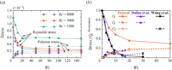
To elucidate that the interaction between LSSs and polymer chains sustains the drag-limiting states, we examined the reduction of Reynolds stresses and the development of polymer stresses as the flow approaches the asymptotic flow state. To that end, the volume-averaged Reynolds stress
 $\tau _{R}^{v}$
and polymer stress
 $\tau _{P}^{v}$
are scrutinized (see figure 10
 $a$
). Evidently, both the Reynolds stress and the polymer stress reach a plateau at sufficiently large
 $Wi$
, indicating saturation of the turbulence dynamics in the MDR state. We quantify the reduction in Reynolds stresses by comparing
 $\tau _{R}^{v}$
in MDR with its Newtonian flow counterpart. Specifically, a reduction in
 $\tau _{R}^{v}$
of up to
 $-52.2\, \%$
,
 $-73.7\, \%$
and
 $-76.0\, \%$
is observed at
 $Re=1500$
,
 $5000$
and
 $8000$
, respectively. These values are comparable to the DR seen in the classical MDR state of the channel/pipe flows (Xi Reference Xi2019) as well as the Reynolds stress reduction in the MDE states of TCF and RPCF (Zhu et al. Reference Zhu, Wan, Lin, Liu, Lu and Khomami2023; Lin et al. Reference Lin, Song, Liu, Wan, Lu and Khomami2024). On the other hand, by comparing
 $\tau _{P}^{v}$
in the MDR state and
 $\tau _{R}^{v}$
in the Newtonian flow field, we observe increased polymer stresses of
 $28.9\, \%$
,
 $20.4\, \%$
and
 $16.2\, \%$
for
 $Re=1500$
,
 $5000$
and
 $8000$
, respectively. Therefore, an estimate of the extent of DR in the MDR state of the viscoelastic TCF can be obtained by adding the reduction of Reynolds stress to the increase in polymer stress. Interestingly, this estimate leads to the DR of
 $-23.3\, \%$
,
 $-53.3\, \%$
and
 $-59.8\, \%$
in sequence for
 $Re=1500$
,
 $5000$
and
 $8000$
, which are close to the “real” DR rate calculated from
 $Nu_{\omega }$
(see figure 1
 $a$
). In general, the above analysis underscores that in this novel MDR state, moderate to high DR can only be achieved, as significant polymer stress and associated drag induced by LSSs (see figures 6
 $d$
and 9) offset the DR resulting from the reduction of Reynolds stress.
This argument is substantiated in figure 10(
 $b$
) by comparing the MDR state in TCF and the classical MDR state in channel flows. Specifically, we extracted Reynolds stress and shear polymer stress from the classical MDR states in comparable friction Reynolds numbers (
 $Re_\tau =181$
,
 $L=120$
in Dallas et al. (Reference Dallas, Vassilicos and Hewitt2010);
 $Re_\tau =189$
,
 $L=100$
in Wang et al. (Reference Wang, Zhang, Wang, Li, Zhang and Li2023);
 $Re_\tau =167$
obtained for
 $Re=5000$
,
 $L=100$
in this study). Results shown in figure 10(
 $b$
) have highlighted the mechanisms for the occurrence of relatively lower DR rates in the MDR state of TCF. On the one hand, the polymer-induced reduction in Reynolds stress (
 $\tau _{R}^{v}$
) is relatively lower for TCF compared with MDR in channel flows, because LSSs persist in generating Reynolds stress (see figure 6
 $d$
); on the other hand, the development of polymer stress (
 $\tau _{P}^{v}$
,
 $\tau _{e2}^{v}$
) is relatively stronger in TCF, because LSSs cause greater polymer stretch (see figures 8 and 9). Note that
 $\tau _P^{v}$
obtained by Dallas et al. (Reference Dallas, Vassilicos and Hewitt2010) in the MDR channel flow absent of LSSs is only slightly smaller than that in the present study, as demonstrated in figure 10(
 $b$
). This may be attributed to the larger
 $L=120$
used in Dallas et al. (Reference Dallas, Vassilicos and Hewitt2010). Hence,
 $\tau _{e2}^{v}$
calculated from Wang et al. (Reference Wang, Zhang, Wang, Li, Zhang and Li2023) also using
 $L=100$
is more comparable to the present study, although
 $\tau _P^{v}$
cannot unfortunately be calculated for comparison by available data.
(
 $a$
) The volume-averaged Reynolds stress and polymer stress for
 $Re$
= 1500, 5000, 8000 calculated as
 $\tau _{R}^{v}=({1}/{d})\int _{R_i}^{R_o}{\langle u_{r}'u_{\theta }' \rangle {\rm d}r}$
and
 $\tau _{P}^{v}=- ({1}/{d})\int _{R_i}^{R_o}{\langle \frac {1-\beta }{Re}\tau _{r\theta } \rangle {\rm d}r}$
, respectively. (
 $b$
) Comparison between MDR in TCF (at
 $Re=5000$
) and classical MDR in channel flow (Dallas et al. Reference Dallas, Vassilicos and Hewitt2010; Wang et al. Reference Wang, Zhang, Wang, Li, Zhang and Li2023). The volume-averaged polymer stress induced by vortical structures, i.e.
 $\tau _{e2}^{v}=-({1}/{d})\int _{R_i}^{R_o}{\langle \frac {1-\beta }{Re}\tau _{r\theta } ^{e2} \rangle {\rm d}r}$
is also plotted. To promote a reasonable comparison between different cases,
 $\tau _{R}^{v}$
,
 $\tau _{P}^{v}$
and
 $\tau _{e2}^{v}$
have been rescaled by the volume-averaged Reynolds stress of corresponding Newtonian turbulent flows.

5. Polymer conformation dynamics
The complete description of the MDR state in TCF requires understanding the variations of the polymer conformation away from its equilibrium state. Most prior studies used variations of isolated components of
 $\unicode{x1D63E}$
or
 $\textrm {trace}(\unicode{x1D63E}\kern1.5pt)$
that are representative of the polymer stretch. However, as suggested by Hameduddin et al. (Reference Hameduddin, Meneveau, Zaki and Gayme2018), such a description is insufficient as the polymer conformation can undergo complex volumetric deformation. Therefore, these authors proposed rigorous scalar measures tailored for characterizing the polymer deformation and its perturbations. Specifically, once a conformation tensor
 $\overline {\unicode{x1D63E}}$
is chosen as a reference, the deformation of polymers can be quantified by the following scalar measures: (i) the logarithmic volume ratio
 $\zeta \equiv \textrm {log}( {\textrm {det}\unicode{x1D63E}}/{\textrm { det}\overline {\unicode{x1D63E}}}\kern1.5pt)$
, which represents the relative expansion or compression with respect to
 $\overline {\unicode{x1D63E}}$
; (ii) the squared geodesic distance
 $\kappa = d^2(\overline {\unicode{x1D63E}},\unicode{x1D63E}\kern1.5pt)\equiv \mathrm { trace[ log^2}(\overline {\unicode{x1D63E}}^{-1/2}\,{\boldsymbol {\cdot }}\,\unicode{x1D63E}\,{\boldsymbol {\cdot }}\, \overline {\unicode{x1D63E}}^{-1/2})]$
, which represents the magnitude of the fluctuations with respect to
 $\overline {\unicode{x1D63E}}$
; (iii) the anisotropy index
 $\xi \equiv \kappa - ({1}/{3})\zeta ^2$
, which represents the deviation of the shape of the polymer from the shape corresponding to the reference tensor
 $\overline {\unicode{x1D63E}}$
. In this paper,
 $\overline {\unicode{x1D63E}}$
is selected as the unit tensor
 $\unicode{x1D644}$
and the log-Euclidean mean conformation tensor
 $\langle \unicode{x1D63E} \kern1.5pt \rangle _{\textrm {log}} \equiv \textrm {exp} ( \langle \textrm {log} \unicode{x1D63E} \kern1.5pt \rangle )$
, to depict the departure of polymer chains from their isotropic equilibrium state (denoted as
 $\zeta _i$
,
 $\kappa _i$
and
 $\xi _i$
) and from the mean flow state (denoted as
 $\zeta _m$
,
 $\kappa _m$
and
 $\xi _m$
), respectively. Here, we employ the log-Euclidean mean as it provides the most physical representation of the ensemble (Hameduddin & Zaki Reference Hameduddin and Zaki2019).
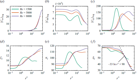
Components of the log-Euclidean mean conformation for the MDR states (
 $Wi=150$
) under different
 $Re$
: (
 $a$
)
 $\langle C_{rr} \rangle _{\textrm {log}}$
, (
 $b$
)
 $\langle C_{\theta \theta } \rangle _{\textrm {log}}$
and (
 $c$
)
 $\langle C_{zz} \rangle _{\textrm {log}}$
. Scalar measures of the conformation tensor: (
 $d$
) the logarithmic volume
 $\zeta _i$
; (
 $e$
) the squared geodesic distance
 $\kappa _i$
; (
 $f$
) the anisotropy index
 $\xi _i$
. Note that here the reference tensor is selected to be the unit tensor
 $\unicode{x1D644}$
that represents the isotropic equilibrium state. Only the inner-half of the gap is shown for clarity.

First, we examine the deformation of the polymer in MDR states in different
 $Re$
, with respect to the isotropic equilibrium state
 $\unicode{x1D644}$
. Figure 11 delineates the wall-normal distributions of the scalar measures mentioned above and the three diagonal components of the log-Euclidean mean conformation. As seen in figure 11(d,e), the distributions of
 $\zeta _i$
and
 $\kappa _i$
are similar because relative to the equilibrium state the polymer expansion and fluctuations are closely related to each other. Specifically, the minimum values of
 $\zeta _i$
and
 $\kappa _i$
occur in the immediate vicinity of the wall (
 $r^+\lt 0.4$
for
 $Re=1500$
and
 $r^+\lt 1$
for
 $Re=5000, 8000$
). As the polymers move away from the wall, they continue to expand and further deviate from the equilibrium state, as evidenced by the increasing values of
 $\zeta _i$
and
 $\kappa _i$
. This behaviour is due to an improved radial and axial polymer stretch (see figure 11
a,c), induced by the increased turbulent fluctuations away from the wall (see figure 6
 $a$
–
 $c$
). However, it should be noted that the streamwise polymer stretch exhibits an overall decrease (figure 11
 $b$
) as it approaches the middle of the gap due to weakening of the mean shear (see figure 1
 $b$
–
 $d$
).
When comparing the MDR states at different
 $Re$
, we observe a notable difference in the position where the maximum values of
 $\zeta _i$
and
 $\kappa _i$
occur. That is,
 $\zeta _i$
and
 $\kappa _i$
peak much closer to the wall (
 $r^+ \approx 2$
) for low
 $Re=1500$
, while they obtain maximum values in the middle of the gap for
 $Re=5000, 8000$
(here,
 $\kappa _i$
for
 $Re=5000$
shows a marginal difference after reaching the peak). This observation is consistent with the spatial distribution of the most energetic POD modes of the polymer conformation tensor field (see figure 9). As discussed above, for the MDR state with
 $Re=1500$
, the well-organized LSSs result in stronger polymer stretch at near-wall boundaries, while at
 $Re=5000,8000$
we observe significant polymer stretch in the centre of the gap. Hence, it is not surprising to see different peak positions for
 $\zeta _i$
and
 $\kappa _i$
at
 $Re=1500$
. In addition, the stretch of the near-wall polymer induced by LSSs occurs mainly in the axial direction, as evidenced by the pronounced peak value of
 $\langle C_{zz} \rangle _{\textrm {log}}$
for
 $Re=1500$
(see figure 11
 $c$
). For all MDR states,
 $\xi _i$
decays away from the wall, indicating the enhanced sphericity of polymers similar to the drag-reducing channel flow (Hameduddin et al. Reference Hameduddin, Meneveau, Zaki and Gayme2018). This is because the increase in polymer stretch in the radial and axial directions leads to a more isotropic conformation tensor. Interestingly, we observe a logarithmic decay law
 $\xi _i =-33 \textrm {ln} r^++90$
by fitting the
 $\xi _i$
profile for a high
 $Re=8000$
in the
 $r^+\gt 10$
region. The physical origin of this decaying law might also be related to the polymer stretch (see weak logarithmic behaviours in figure 11
 $a$
–
 $c$
). Nevertheless, future studies should examine this trend, particularly in regard to the strict theoretical relationship between polymer stretch and the anisotropy of polymer conformation.
(
 $a$
) The squared geodesic distance
 $\kappa _m$
for the MDR states (
 $Wi=150$
) under different
 $Re$
. Note that here the reference tensor is selected to be the log-Euclidean mean conformation. Only the inner-half of the gap is shown for clarity. (
 $b$
) Probability density function of
 $\kappa _m$
sampling at different radial positions in the MDR state with
 $Re=1500$
.

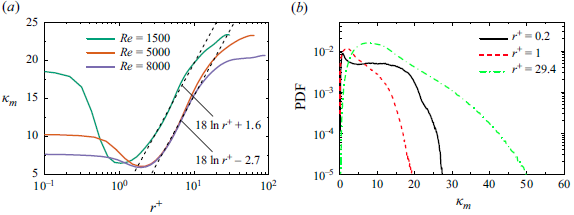
We have also examined the deformation of the polymer relative to the mean state
 $\langle \unicode{x1D63E}\rangle _{\textrm {log}}$
. We have depicted the profiles of
 $\kappa _m$
, because: (i) the volumetric expansion and compression relative to
 $\langle \unicode{x1D63E}\rangle _{\textrm {log}}$
is symmetric, that is, the mean value of
 $\zeta _m$
is zero; and (ii) the anisotropy index
 $\xi _m$
is just a function of
 $\zeta _m$
and
 $\kappa _m$
, which is equal to
 $\kappa _m$
in this case. Figure 12(
 $a$
) shows a strong similarity between the distribution of
 $\kappa _m$
in MDR states of different
 $Re$
, indicating a universal polymer fluctuation dynamics in MDR states of viscoelastic turbulent TCF. Specifically,
 $\kappa _m$
decays as polymers move away from the wall and then attains a local minimum at
 $r^+\approx 1$
for
 $Re=1500$
and at
 $r^+\approx 2$
for
 $Re=5000, 8000$
. Subsequently, it exhibits a logarithmic growth and eventually reaches a peak value at the middle of the gap. A similar variation of
 $\kappa _m$
, namely, an appreciable near-wall drop exists in drag-reducing channel flows (Esteghamatian & Zaki Reference Esteghamatian and Zaki2020). Also, it is interesting to note that the logarithmic law of
 $\kappa _m$
for different MDR states shares an identical slope, that is,
 $\kappa _m=18\textrm {ln}r^+ + B$
, with
 $B=1.6$
for
 $Re=1500$
and
 $B=-2.7$
for
 $Re=5000, 8000$
. This slope value is specific to viscoelastic TCF studies, and its universality remains an open question.
The joint probability density function (JPDF) of the logarithmic volume ratio
 $\zeta _m$
and the squared geodesic distance
 $\kappa _m$
for the MDR states (
 $Wi=150$
) at
 $(a)$
 $Re=1500$
,
 $(b)$
 $Re=5000$
and
 $(c)$
 $Re=8000$
. Note that here the reference tensor is selected to be the log-Euclidean mean conformation. The grey and green line contours refer to radial locations at the near-wall position (
 $r^+=1$
) and at the middle of gap, respectively. For all plots, eight contour levels in a log range of [
 $10^{-9},10^{-3}$
] are used. The red dashed line denotes the realizability bound
 $\kappa _m=(1/3)\zeta _m^2$
, derived in Hameduddin et al. (Reference Hameduddin, Meneveau, Zaki and Gayme2018).

In the MDR state
 $Re=8000$
, although polymers undergo a larger conformation deviation from the equilibrium in the middle of the gap (figure 11
 $e$
), their departure from the mean state is smaller than that of smaller
 $Re$
. To gain more insight into the spatial distribution of the polymer deformation fluctuations, we examine the probability density function (PDF) of
 $\kappa _m$
sampling at three prototypical radial positions. Only the PDFs for
 $Re=1500$
are depicted for brevity, since the results at other
 $Re$
are similar. As seen in figure 12(
 $b$
), the peak of PDF values shifts to larger
 $\kappa _m$
as
 $r^+$
increases. This is once again due to the fact that the turbulent fluctuations are more intense as one approaches the middle of the gap. This in turn creates more events with stronger polymer deformation fluctuations. Moreover, by comparing the PDF distributions for
 $r^+=0.2$
and
 $r^+=1$
one can rationalize the occurrence of the local minimum observed in figure 12(
 $a$
). Specifically, an abundance of extreme-valued events (e.g.
 $\kappa _m\gt 20$
) is observed at
 $r^+=0.2$
, which in turn results in higher mean values of
 $\kappa _m$
in the immediate vicinity of the wall (
 $r^+\lt 1$
for
 $Re=1500$
and
 $r^+\lt 2$
for
 $Re=5000,8000$
). To that end, in the wall vicinity, the fluctuation of the wall shear can produce events with extreme-valued polymer deformation fluctuations.
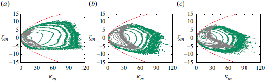
To further scrutinize the dynamics of the polymer conformation in the MDR state, we have calculated the JPDF of
 $\zeta _m$
and
 $\kappa _m$
relative to
 $\langle \unicode{x1D63E}\rangle _{\textrm {log}}$
. The shape of JPDF is symmetric about
 $\zeta _m=0$
; although a slight asymmetry is evident at higher
 $Re$
, they correspond to rare events. This is consistent with the fact that the polymer expansion and compression are symmetric with respect to the mean state. The most extreme excursions of polymers away from the mean occur in the middle of the gap where the turbulence fluctuations are stronger (see figure 6
 $d$
). Moreover, comparing different MDR states reveals a greater area in the
 $(\zeta _m,\kappa _m)$
plane at the middle of the gap for
 $Re=1500$
, which shows events with up to
 $\kappa _m=105$
. This provides concrete evidence that, although the LSSs are well organized at
 $Re=1500$
, they can lead to a larger polymer departure from the mean state.
6. Influence of the maximum chain extensibility on asymptotic drag states
Recent studies have shown that maximum chain extensibility plays a key role in drag-reducing planar shear flows. Specifically, it can alter the relaminarization transition threshold in viscoelastic pipe flows (Lopez et al. Reference Lopez, Choueiri and Hof2019) or influence the essence of the classical MDR state in channel flows (Wang et al. Reference Wang, Zhang, Wang, Li, Zhang and Li2023). Therefore, in this section, we have conducted simulations at
 $Re=5000$
with smaller
 $L=50$
and larger
 $L=200$
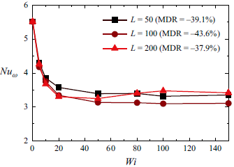
to examine the influence of maximum chain extensibility on the novel MDR state of TCF. As shown in figure 14, we observe different degrees of DR with different
 $L$
, evidenced by the limiting behaviour of
 $Nu_{\omega }$
in sufficiently large
 $Wi$
. Interestingly, the DR rate in the MDR state shows a non-monotonic dependence on the maximum chain extensibility. We observe the highest DR (
 $-43.6\, \%$
) in a moderate
 $L=100$
; while at smaller
 $L=50$
and larger
 $L=200$
, we observe lower DR rates of
 $-39.1\, \%$
and
 $-37.9\, \%$
, respectively. This further highlights that elastically induced DR in the MDR state of TCF is still not as efficient as that of channel/pipe flows. Although the extents of DR at
 $L=50$
and
 $L=200$
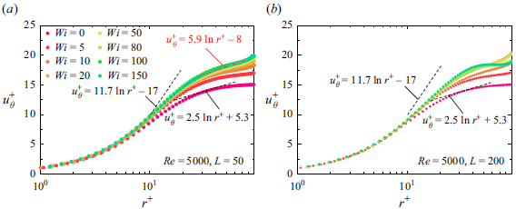
are remarkably close, the mean velocity profiles
 $u_{\theta }^+$
demonstrate a different behaviour at high
 $Wi$
. Specifically, for the MDR state with
 $L=50$
a logarithmic-like law
 $u_{\theta }^+=5.9 \textrm {ln} r^+ -8$
can be obtained by fitting the profile
 $u_{\theta }^+$
in the region
 $r^+\geqslant 30$
(see figure 15
 $a$
). However, the gradient of
 $u_{\theta }^+$
is negative in the bulk for the MDR state with
 $L=200$
(see figure 15
 $b$
). This clearly indicates that the maximum chain extensibility plays a significant role in determining the flow dynamics of the MDR states in TCF. To this end, in the following we will discuss in detail the
 $L$
-induced alteration of turbulence dynamics in MDR states.
Nusselt number
 $Nu_{\omega }$
versus
 $Wi$
at various
 $L$
with
 $Re=5000$
.

The log plots of mean velocity profile
 $u_{\theta }^{+}$
in the inner-half of the gap versus wall-normal distance
 $r^+$
for (
 $a$
)
 $L=50$
and (
 $b$
)
 $L=200$
with
 $Re=5000$
.

Space–time plots of radial velocity
 $u_r$
along axial sampling lines near the inner wall
 $(a,d,g)$
, at the middle of gap
 $(b,e,h)$
and near the outer wall
 $(c,f,i)$
for the MDR states (
 $Wi=150$
) with
 $L=50$
 $(a,b,c)$
,
 $L=100$
 $(d,e,f)$
and
 $L=200$
 $(g,h,i)$
at
 $Re=5000$
. To provide a better illustration, here
 $u_r^i$
,
 $u_r^m$
and
 $u_r^o$
have been used to denote the radial velocities near the inner wall, at the middle of gap and near the outer wall, respectively.

We examined the influence of the maximum extensibility of the chain on the flow structures of MDR states through the space–time plots shown in figure 16. Basically, increasing
 $L$
results in more structured and organized flow patterns. Specifically, at
 $L=50$
we observed a large number of intense inflow/outflow spots across the gap at MDR (see figure 16
 $a$
–
 $c$
), indicating that small-scale structures primarily drive the flow dynamics. For
 $L=100$
, as previously discussed, two pairs of large-scale Taylor vortices become apparent due to the polymer-induced suppression of small-scale motions. This characteristic is particularly evident in the near-wall regions (see figure 16
 $d$
,
 $f$
), while the flow pattern in the middle of the gap still exhibits a high degree of randomness. In fact, we observe the most organized flow patterns at
 $L=200$
. This is due to the continued suppression of small-scale structures. In addition, the space–time plots clearly delineate the presence of three pairs of LSSs spanning the gap (see figure 16
 $g$
–
 $i$
). Compared with
 $L=100$
, a higher maximum chain extensibility (
 $L=200$
) further weakens the randomness of the flow in the middle of the gap. In general, increasing
 $L$
in the MDR states of TCF leads to structural changes, namely weakening and improving the dominance of small- and large-scale structures, respectively. It should be noted that for the MDR state in channel flow, Wang et al. (Reference Wang, Zhang, Wang, Li, Zhang and Li2023) had also found a structural change related to
 $L$
, namely, small
 $L$
results in marginal inertial turbulence containing hairpin vortex structures, while large
 $L$
excites EIT characterized by cylindrical structures oriented spanwise. Clearly, the above
 $L$
-induced structural changes are different as here the MDR state contains LSSs. Nevertheless, increasing the maximum chain extensibility alters the dominant flow dynamics in MDR states of TCF.
Instantaneous isosurfaces of the decomposed streamwise velocity fluctuations coloured by the corresponding decomposed radial velocity fluctuations at the MDR states (
 $Wi=150$
) with
 $Re=5000$
: (
 $a,c,e$
) for
 $u_{\theta ,l}'$
and (
 $b,d,f$
) for
 $u_{\theta ,s}'$
, whereas (
 $a,b$
) for
 $L=50$
, (
 $c,d$
) for
 $L=100$
and (
 $e,f$
) for
 $L=200$
. For all the plots,
 $u_{\theta ,l}'=$
 $u_{\theta ,s}'=0.05$
.

Balance of angular momentum current across the gap for the MDR state (
 $Wi=150$
) of (
 $a$
)
 $L=50$
, (
 $b$
)
 $L=100$
and (
 $c$
)
 $L=200$
, with
 $Re=5000$
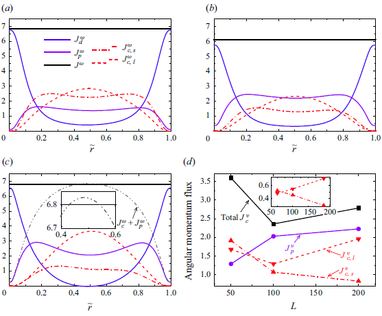
. Here,
 $J^{\omega }_d= -({r^3\beta }/{Re})({\partial \langle \omega \rangle }/{\partial r})$
and
 $J^{\omega }_p= -({r^3( 1-\beta )}/{Re})({\langle \tau _{r\theta } \rangle }/{r})$
represent the diffusive flux, and the elastic source/sink, respectively, while the convective flux
 $J^{\omega }_c=r^3\langle u_r\omega \rangle$
has been decomposed into large- and small-scale parts. In panel (
 $c$
), the inset shows the zoom-in of the centre region of the gap. (
 $d$
) Volume-averaged angular momentum fluxes as a function of
 $L$
, for the MDR state (
 $Wi=150$
) with
 $Re=5000$
. Here, the volume-averaged values are calculated by the integral across the gap, e.g.
 $J_{c}^{v}=({1}/{d})\int _{R_i}^{R_o}{ J_{c}^{\omega } {\rm d} r}$
. Inset in panel (
 $d$
) depicts the variation of decomposed
 $J_{c}^{v}$
, which has been rescaled by the total
 $J_{c}^{v}$
at each
 $L$
.

To quantify turbulence fluctuations induced by different flow structures, we use a decomposition method based on a filter operation (Motoori & Goto Reference Motoori and Goto2021; Motoori, Wong & Goto Reference Motoori, Wong and Goto2022). Specifically, turbulent motions are decomposed into large- and small-scale velocity fluctuations, denoted as
 $\boldsymbol {u}_{l}'$
and
 $\boldsymbol {u}_{s}'$
, respectively. They are strictly separated in the Fourier space by implementing filter operations, with low- and high-pass filters for
 $\boldsymbol {u}_{l}'$
and
 $\boldsymbol {u}_{s}'$
, respectively. It is noted that the filters are only applied in the axial direction, as different flow structures are characterized by their axial wavelengths. To this end, the filtering scale
 $k_z^{filter}$
is carefully chosen according to the axial wavelengths of LSSs (see Appendix A). As depicted in figure 17, the implemented filter operation has faithfully decomposed flow structures at different scales. Moreover, the reduction in the number of flow structures visualized by the isosurfaces of
 $u_{\theta ,s}'$
clearly points to a significant weakening of small-scale SEVs with increasing
 $L$
(see figure 17
b,d,f), consistent with the observation in figure 16.
Since we decompose the large- and small-scale structures as outlined above, one can ascertain how these structures contribute to angular momentum transport. To answer this question, we decompose the convective flux
 $J^{\omega }_c=r^3 \langle u_r\omega \rangle$
into the large- and small-scale components (denoted as
 $J^{\omega }_{c,l}$
and
 $J^{\omega }_{c,s}$
, respectively) using the decomposed velocity fluctuations. As depicted in figure 18, the balance of the angular momentum current across the gap is maintained for all MDR states with different
 $L$
, justifying the applied decomposition. By increasing
 $L$
, the resulting modifications of angular momentum transport can be summarized as
 $J^{\omega }_{c,s}$
is weakened, while
 $J^{\omega }_p$
is enhanced and
 $J^{\omega }_{c,l}$
depicts a non-monotonic variation, as evidenced by figure 18(
 $a$
–
 $c$
). Specifically, we see a continuous reduction from 2.5 to 1 in the peak value of
 $J^{\omega }_{c,s}$
, while the peak value of
 $J^{\omega }_{c,l}$
decreases from 2.8 to 2.3 before increasing to 3.5. Meanwhile, due to the efficient polymer chain stretch induced by the well-organized LSSs with increased elasticity (
 $L=50\to 200$
), the maximum value of
 $J^{\omega }_p$
increases from 1.5 to 3. Interestingly, for the MDR state at
 $L=200$
, the sum of angular momentum currents induced by Reynolds and polymer stresses has exceeded the total current in the centre region of the gap (see the inset of figure 18
 $c$
), which is reminiscent of the situation in weak rotation RPCF where significant Reynolds stress exceeds total stress (Salewski & Eckhardt Reference Salewski and Eckhardt2015). This sum of the overshot of
 $J^{\omega }_p$
and
 $J^{\omega }_c$
gives rise to the negative
 $u_\theta ^+$
gradient observed in figure 15(
 $b$
), and is attributed to the efficient transverse angular momentum transport induced by well-organized LSSs (Song et al. Reference Song, Teng, Liu, Ding, Lu and Khomami2019).
To highlight the underlying mechanisms of the non-monotonic behaviour of the MDR rate as
 $L$
increases, we calculate the volume-averaged values of different angular momentum currents as a function of
 $L$
. As depicted in figure 18(
 $d$
), the competition between various angular momentum transport mechanisms results in the dependence of the DR rate on
 $L$
. Basically,
 $J^v_p$
monotonically increases with increasing
 $L$
, while
 $J^v_c$
reaches a minimum at
 $L=100$
. Hence, the non-monotonic behaviour of
 $J^v_c$
is responsible for the occurrence of a most efficient MDR state in TCF. By decomposing
 $J^v_c$
into large- and small-scale parts, it is further shown that the non-monotonic variation of
 $J^v_{c,l}$
accounts for the non-monotonic total
 $J^v_c$
. Specifically,
 $J^v_{c,l}$
is relatively larger in
 $L=50,200$
, because the corresponding MDR states have a larger number of Taylor rolls (Martínez-Arias et al. Reference Martínez-Arias, Peixinho, Crumeyrolle and Mutabazi2014), i.e. three pairs in
 $L=50,200$
and two pairs at
 $L=100$
as depicted in figure 17(a,c,e). On the other hand,
 $J^v_{c,s}$
continuously decreases with increasing
 $L$
, indicating that larger
 $L$
suppresses SEVs more significantly (Wang et al. Reference Wang, Zhang, Wang, Li, Zhang and Li2023). Consequently, though both MDR states at
 $L=50,200$
exhibit higher flow drags compared with
 $L=100$
, the underlying mechanisms are different. For
 $L=50$
, both small-scale incoherent and large-scale coherent transports contribute to a higher flow drag. However, increasing
 $L$
from 100 to 200 further refines the LSSs, contributing to stronger large-scale coherent transport and, in turn, resulting in higher flow drag.
7. Concluding remarks
To explore polymer-induced drag-limiting states, we performed extensive DNS of low-curvature TCF (
 $\eta =0.99$
) of dilute polymeric solutions. Specifically, by gradually increasing
 $Wi$
from 0 to 150 within the Reynolds number range of
 $Re=1500\sim 8000$
, we demonstrate the existence of a novel MDR state in turbulent wall-bounded flows containing LSSs. The novelties of the observed asymptotic MDR state are as follows. Even at an exceedingly high
 $Wi$
, the degree of DR for the realized MDR states is not as high as that for classical MDR states (parallel wall-bounded flows) at comparable friction Reynolds numbers, thus preventing the mean velocity profile from reaching the well-known Virk asymptote. Moreover, in contrast to the sole presence of small-scale vortices typically observed in the MDR of channel/pipe flows, the flow structures consist of LSSs that coexist with small-scale SEVs. These LSSs persist on the way to MDR in low-curvature TCF, as revealed qualitatively by the evolution of space–time plots and quantitatively by the TKE spectra.
We have also thoroughly investigated the turbulence dynamics of this novel MDR state, with particular focus on those associated with LSSs. It is observed that the polymer elasticity leads to suppression of SEVs, and stabilization as well as weakening of LSSs, leading to reduced Reynolds stresses and a commensurate DR. However, the polymer-induced reduction of Reynolds stress is lower than the classical MDR in channel/pipe flows, because LSSs always persist and contribute to the generation of Reynolds stress. On the other hand, we demonstrate that the interaction between vortical structures and polymers leads to a significant development of polymer stress. Moreover, POD analysis of the velocity and polymer conformation fields reveals that this development is ostensibly due to LSSs, particularly their ability to stretch polymers dramatically at the vortical boundaries. The drag-limiting state arises from both the asymptotic behaviours of Reynolds stress reduction and polymer stress development. Therefore, the remanence of Reynolds stress and the strong polymer stress induced by the distinct flow structures in TCF combine to result in an MDR state with lower DR extent than in channel and pipe flows.
To provide a complete description of the novel MDR state, we carefully examine the deformation of the polymer using the scalar measures proposed by Hameduddin et al. (Reference Hameduddin, Meneveau, Zaki and Gayme2018). For all MDR states at varying
 $Re$
, the intense wall shear generates a large polymer deformation in the immediate vicinity of the wall. As the polymers move away from the wall, typically they further accumulate expansion and deviate from the equilibrium state because of the gradual enhancement of turbulent fluctuations. However, the different behaviour of the LSSs results in different peak positions of
 $\zeta _i$
and
 $\kappa _i$
, where the deviation is the farthest from the equilibrium states. That is, well-organized LSSs in the MDR state at
 $Re=1500$
result in pronounced axial polymer stretching, and hence larger polymer deformation, in the near-wall regions. Relative to the mean state, the polymer deformation fluctuation quantified by squared geodesic distance displays a universal behaviour at the MDR states of TCF, i.e.
 $\kappa _m$
decays to attain a local minimum as polymers move away from the wall and subsequently reaches a peak value in the middle of the gap with identical-slope logarithmic growth.
Furthermore, we investigated the role of
 $L$
on the flow dynamics of the MDR state in TCF by conducting additional simulations with smaller
 $L=50$
and larger
 $L=200$
at
 $Re=5000$
. The extents of DR in different MDR states show a non-monotonic dependence on
 $L$
. Within the present parameter range, the most efficient DR occurs in the moderate range
 $L=100$
. Examination of flow structures indicates that the
 $L$
-induced structural changes lead to weakening the dominance of small-scale structures and non-monotonic variation of the number of large-scale Taylor rolls. This observation is further quantitatively verified by the variation of small- and large-scale convective fluxes, which are obtained from a strict decomposition method based on filter operations. Moreover, on the basis of the balance of angular momentum transport, the underlying mechanism for the non-monotonic behaviour of the MDR rate is discussed. Specifically, the MDR state at
 $L=50$
exhibits a higher flow drag because both small-scale incoherent and large-scale coherent transports are stronger compared with
 $L=100$
. However, LSSs are enhanced by increasing
 $L$
from 100 to 200, resulting in a higher flow drag via the stronger large-scale coherent transport.
In summary, present DNS results demonstrate for the first time the existence of an asymptotic MDR state in low-curvature turbulent TCF containing LSSs. A comprehensive examination of this novel MDR state has enabled elucidation of the intriguing turbulence dynamics, and polymer deformations as well as the influence of maximum chain extensibility. Considering the previous findings of MDE, this study provides concrete evidence for our earlier postulation that polymer-induced asymptotic behaviours are an inherent property of viscoelastic wall-bounded turbulent flows. Hence, it is rational to assume that asymptotic drag-limiting states with arbitrary DM can be achieved by combining the mechanisms of polymer stress development and Reynolds stress reduction, which would be a further motivation of our future work to explore the physical origin underlying such asymptotic flow states from the perspective of polymer–turbulence interaction.
Acknowledgements.
The calculations were completed on the supercomputing system in the Supercomputing Center at the University of Science and Technology of China.
Funding.
This work was supported by the National Natural Science Foundation of China through grant numbers 12388101, 12402257, 12172353, 92252202; the Science Challenge Project; the Postdoctoral Fellowship Program of CPSF under grant number GZC20232551; and National Science Foundation CBET0755269.
Declaration of interests.
The authors report no conflict of interest.
Appendix A. Verification of the computational domain
A rigorous test of the adequacy of the size of the computational domain is provided by the two-point autocorrelation functions, which are defined as
 \begin{equation} R_{\theta \theta }(\unicode{x0394} x)=\frac {\langle u'_{\theta }(r,\theta ,z,t)u'_{\theta }(r,\theta ,z+\unicode{x0394} x,t) \rangle }{\langle {u'_{\theta }}^{2}(r,\theta ,z,t)\rangle }, \end{equation}
where
 $\unicode{x0394} x$
denotes spatial separation. In our case, this corresponds to
 $\unicode{x0394} z$
and
 $\unicode{x0394} \theta$
since we are interested in examining the correlation of streamwise velocity fluctuation in axial and azimuthal directions, respectively. Previously, we have shown that computational domains that are not sufficiently long lead to a large value of
 $R_{\theta \theta }$
, i.e.
 $R_{\theta \theta }$
cannot decay to zero, as one cannot capture the largest turbulence scales with the selected domain (Li et al. Reference Li, Sureshkumar and Khomami2006). To do this, we have calculated
 $R_{\theta \theta }$
for all MDR states achieved at
 $Wi=150$
for each (
 $Re, L$
). As depicted in figure 19, the quasiperiodicity of
 $R_{\theta \theta }(\unicode{x0394} z)$
signifies the LSSs stacked in the axial direction, and
 $R_{\theta \theta }(r\unicode{x0394} \theta )$
rapidly drops to zero for all curves, which suggests that the azimuthal computational domain is sufficiently long. Moreover,
 $R_{\theta \theta }(r\unicode{x0394} \theta )$
recovers to zero except for
 $(Re, L)=(1500, 100)$
and (
 $5000, 200$
). This is because in these two cases the well-organized LSSs are spanning the full azimuthal length of the computational domain, as indicated by figures 2(
 $f$
) and 16(
 $g$
–
 $i$
). In addition, the axial length scale of the LSSs can be analysed from
 $R_{\theta \theta }(\unicode{x0394} z)$
along the axial direction. As suggested by Dong (Reference Dong2008), velocity fluctuations negatively correlate in an azimuthal vortex tube. Therefore, the first minimum of
 $R_{\theta \theta }(\unicode{x0394} z)$
is commonly used to evaluate the axial length scale of the vortex tube. As shown in figure 19(
 $a$
), the axial separations of the first minimum in
 $R_{\theta \theta }(\unicode{x0394} z)$
are found to be
 $1.17$
,
 $3.06$
and
 $2.55$
in sequence for
 $(Re, L)=(1500, 100)$
, (
 $5000, 100$
) and (
 $8000, 100$
). These values correspond to approximately
 $5$
,
 $2$
and
 $2$
pairs of LSSs, respectively, consistent with the dominant spatial modes depicted in figure 5. Overall, examination of two-point correlations along the axial and azimuthal directions has shown that the chosen computational domain is sufficient to obtain reasonable turbulence statistics.
Appendix B. Grid convergence study
Two-point autocorrelation functions at the middle of gap (
 $\tilde {r}=0.5$
) for streamwise velocity fluctuation in (
 $a$
) axial and (
 $b$
) azimuthal direction. All curves correspond to the MDR states achieved at
 $Wi=150$
for each (
 $Re, L$
). Here, the first minimum of
 $R_{\theta \theta }(\unicode{x0394} z)$
is marked with triangle.

Profiles of r.m.s. values of (
 $a$
) velocity components and (
 $b$
) polymer stresses at
 $Re=5000, L=200, Wi=150$
with various mesh sizes.

Simulations of viscoelastic turbulent flows are extremely challenging due to the necessity to accurately resolve the polymeric stresses. Therefore, to scrutinize the precision of our simulation results, we performed a grid convergence study using the parameter set that corresponds to flows with the largest elastic effect, i.e.
 $L=200, Wi=150$
. Specifically, we implemented two additional mesh sizes, namely coarser and refined grids of
 $N_{r}\times N_{\theta } \times N_{z}=64\times 384\times 384$
and
 $192\times 512\times 512$
, respectively. As shown in figure 20, the profiles of the r.m.s. values of the velocity components and the polymer stresses confirmed the precision of the reported results. Overall, both velocity and polymer stress fields attain excellent grid convergence with increasing spatial resolution. That is, the results for the predicted velocity and polymer stress fields do not show noticeable differences for the two finer grids. It is also a clear indication that the flow dynamics discussed in this study do not suffer from the recently reported polymer diffusive instability (Beneitez, Page & Kerswell Reference Beneitez, Page and Kerswell2023; Couchman et al. Reference Couchman, Beneitez, Page and Kerswell2024). The more or less identical polymer stress fields obtained with different ‘numerical dissipation’ (grid resolution; see figure 20
 $b$
) unequivocally support this assertion.
Appendix C. Examination of the TCF flow regimes
It has been well documented that the turbulent Newtonian TCF can be categorized into the classical (transitional) turbulent regime and the ultimate regime (Grossmann et al. Reference Grossmann, Lohse and Sun2016). In the classical regime, turbulence develops mainly in the bulk, while the boundary layers (BLs) are still of the laminar type. By increasing driving force, the flow enters the ultimate regime, which is characterized by turbulent BLs, with the bulk being turbulent Taylor vortices or featureless turbulent flows. We have carried out an analysis of the BL dynamics to determine which regime the TCF in this study belongs to (particularly for
 $Re=8000$
). Specifically, we have plotted the instantaneous azimuthal velocity in the
 $r$
–
 $z$
plane. As depicted in figure 21(
 $a$
), the plumes are not ejected from the entire boundary (Ostilla-Mónico et al. Reference Ostilla-Mónico, van der Poel, Verzicco, Grossmann and Lohse2014b
), so the BLs are still laminar-type for all the
 $Re$
considered. To this end, the angular velocity profiles can be decomposed into the bulk and two BLs, as illustrated in figure 21(
 $b$
). It should be noted that although the bulk profile of
 $\langle \omega \rangle / \Omega$
is flatter with increasing
 $Re$
, the linear fit to the bulk part still shows a slight angular velocity gradient due to the low curvature. In fact, the fitting function is given as
 $\langle \omega \rangle / \Omega = -0.05 \tilde {r}+0.51$
for the present simulations (
 $Re=8000$
). Moreover, the measurement of the BL thickness further demonstrates laminar-type BLs. We define BL thickness
 $\delta$
as the depth where the linear fit to the
 $\langle \omega \rangle / \Omega$
profile near the wall intersects the linear fit to the profile mid-depth (Ostilla-Mónico et al. Reference Ostilla-Mónico, Stevens, Grossmann, Verzicco and Lohse2013). As seen in the inset of figure 21(
 $b$
), the scaling of
 $\delta$
closely follows the Prandtl–Blasius prediction for laminar BLs, i.e.
 $\delta \sim Re^{-0.5}$
(Landau & Lifshitz Reference Landau and Lifshitz1987). Overall, the analysis presented above has shown that the investigated TCFs are in the classical (transitional) regime, characterized by laminar BLs and turbulent Taylor vortices in the bulk.
(
 $a$
) Snapshots of the azimuthal velocity
 $u_\theta$
for Newtonian fluids at various
 $Re$
. Only
 $0\leqslant z \leqslant \pi$
are shown for clarity. (
 $b$
) Angular velocity profiles for Newtonian fluids at various
 $Re$
. The black dashed lines are an illustration of the laminar BLs, while the black dashed–dotted line shows a linear fit to the bulk part of
 $\langle \omega \rangle / \Omega$
. The inset depicts the variation of BL thickness
 $\delta$
as a function of
 $Re$
.

Appendix D. Comparison with other asymptotic DR states
To examine the possibility of experiments to obtain the MDR state shown in this study, we carried out a comparison between the present numerical results and available experimental data. Before conducting the analysis, we must emphasize that a quantitative comparison of numerical simulations and experiments is challenging for viscoelastic flows, due to the following aspects: (i) the polymer constitutive equation models such as the FENE-P model are not a fully accurate representative of actual dilute polymeric solutions (Larson & Desai Reference Larson and Desai2015); (ii) the simulation protocol is difficult to match in experiments. That is, the MDR state is usually obtained by increasing
 $Wi$
in numerical simulations. Although experiments must keep the elasticity number (
 $El=Wi/Re$
) fixed, the MDR state at a fixed
 $Re$
can only be achieved by increasing the polymer concentrations (Procaccia, L’vov & Benzi Reference Procaccia, L’vov and Benzi2008; Xi Reference Xi2019). However, the qualitative comparison made here may highlight the present MDR state as a distinctive piece in the puzzle ‘phase spaces’ of various asymptotic MDR and MDE states in different flow configurations.
(
 $a$
) Friction factor
 $C_f$
as a function of
 $Re$
. For TCF,
 $C_f$
is calculated as
 $[(1-\eta )^2/\pi ]G/Re^2$
, with
 $G$
being the dimensionless torque (Lathrop, Fineberg & Swinney Reference Lathrop, Fineberg and Swinney1992; Grossmann et al. Reference Grossmann, Lohse and Sun2016). The dashed–dotted lines indicate the power-law scaling for
 $C_f$
. (
 $b$
) The DR rate for various flow geometries. For consistency, here the definition of DR is based on
 $C_f$
, namely,
 $DR^*=1-C_f/C_f^{N}$
, with
 $C_f^{N}$
being the friction factor for Newtonian fluids. Circles, numerical simulation for TCF at
 $\eta =0.99$
; triangles, experiments for TCF at
 $\eta =0.714$
using two different polyacrylamide polymers (Zhang et al. Reference Zhang, Fan, Su, Xi and Sun2025); solid squares, numerical simulation for channel flow conducted by Wang et al. (Reference Wang, Zhang, Wang, Li, Zhang and Li2023) (note that these authors used a
 $Wi$
range of
 $1\sim 60$
); hollow squares, numerical simulation for channel flow conducted by Dallas et al. (Reference Dallas, Vassilicos and Hewitt2010) (note that these authors used a
 $Wi$
range of
 $2\sim 17$
); dashed lines, experiments for typical parallel-shear turbulent flows (Owolabi, Dennis & Poole Reference Owolabi, Dennis and Poole2017).

Specifically, we have compared the friction factor
 $C_f$
in
 $\eta =0.99$
with the experiment data obtained in
 $\eta =0.714$
(Zhang et al. Reference Zhang, Fan, Su, Xi and Sun2025). As depicted in figure 22(
 $a$
),
 $C_f$
for
 $5\leqslant Wi\leqslant 20$
closely follows the power-law scaling
 $C_f \sim Re^{-0.58}$
found in the experiments. An increase in
 $Wi$
leads to a steeper scaling law of
 $C_f \sim Re^{-0.69}$
, provided that the present numerical simulations consider a limited range of
 $Re$
. It is worth noting that in experiments with a smaller
 $\eta$
, the wavelength and pattern of the large-scale Taylor vortices are not changed compared with the Newtonian cases. Hence, the present change in scaling (
 $Re^{-0.58} \to Re^{-0.69}$
) can be attributed to the fact that the wavelength and pattern of LSSs have been significantly modified for large
 $Wi$
, as seen from figures 2–5. In fact, the largest
 $Wi$
achieved in the experiments by Zhang et al. (Reference Zhang, Fan, Su, Xi and Sun2025), is only approximately 30 (at
 $Re=2.5\times 10^4$
). Although the scaling exponents for TCF are close to those for pipe flow (as summarized by Virk et al. (Reference Virk, Mickley and Smith1970),
 $C_f=0.59Re^{-0.58}$
), the DR rate is relatively lower for TCF (both in experiments and numerical simulations). To provide a clear illustration of this point, we have summarized the DR rate for different flow geometries in figure 22(
 $b$
). We again emphasize the difference in protocols between numerical simulations and experiments (Procaccia et al. Reference Procaccia, L’vov and Benzi2008; Xi Reference Xi2019). Hence, the MDR rates obtained by numerical simulations of channel flow exceed those obtained by experiments. Nevertheless, it is seen that the MDR states in TCF at
 $\eta =0.99$
have lower DR rates compared with those for parallel-shear turbulent flows (especially those obtained by numerical simulations), consistent with the arguments we made in the main text. This plot also provides an indication that the geometry curvature may play a significant role in determining the DR rate of MDR states. For
 $\eta =0.714$
, high curvature may have led to stronger Taylor vortices. On the one hand, their contribution to angular momentum transport is significant (Zhang et al. Reference Zhang, Fan, Su, Xi and Sun2025). However, they stretch the polymer more violently, leading to larger polymer stress. These two aspects result in a much lower DR rate (
 $\sim -20\, \%$
). For
 $\eta =0.99$
, centrifugal-force-induced Taylor vortices are weaker and the contribution of small-scale SEVs is more significant. This makes the flow more like parallel-shear flows. However, the MDR rate obtained for low-curvature TCF is still lower than that for parallel-shear flows, because of the persistence of LSSs. In general, exploring different asymptotic drag-limiting states in various flow configurations can be an interesting topic for future work on polymer-induced drag modification in wall-bounded turbulent flows.