2 Statement of the problem

Let us consider a semi-bounded volume of a liquid and the same volume of its vapour (see figure 1). The phases differ from each other by their densities $\unicode[STIX]{x1D70C}_{j}$ and also by the coefficients of kinematic viscosity, $\unicode[STIX]{x1D708}_{j}$ , thermal conductivity, $\unicode[STIX]{x1D705}_{j}$ , and thermal diffusivity, $\unicode[STIX]{x1D712}_{j}$ . Hereinafter, the index $j$ refers to the liquid ( $j=1$ ), its vapour ( $j=2$ ), or both the phases. The main case studied in the present paper is water and water vapour at atmospheric pressure and the corresponding saturation temperature $100\,^{\circ }\text{C}$ (see table 1). So, the ratio of the liquid density to that of its vapour is taken much greater than the corresponding ratio of the coefficients of their kinematic viscosities, which is also large. The ratio of the thermal conductivity coefficients of the liquid and its vapour is much greater than unity. In addition to water, many substances, for example ethanol and its vapour, possess similar properties far from their critical point (see Vargaftik, Vinogradov & Yargin Reference Vargaftik, Vinogradov and Yargin1996).

The two-layer, two-phase system described above is subjected to a field of gravity with the acceleration vector $\boldsymbol{g}$ , which is directed down towards the volume occupied by the heavy liquid. The Rayleigh–Taylor instability is absent. Also, there is permanent, homogeneous subcooling from the side of the liquid and the same heating from the side of its vapour. As is well known, heating from above does not cause thermogravity convection. The formulation of the problem allows a stationary base state with a flat liquid–vapour interface under the pressure $p_{0}$ and at the saturation temperature $T_{s0}$ , characterized by the coefficient of surface tension, $\unicode[STIX]{x1D6FE}$ , and the specific heat of vapour formation, $L$ . Further, as a control parameter, we will use the heat flux $q$ transferred in the process of thermal conductivity through the unperturbed layers of the phases.

Figure 1.

Configuration and parameters of the system.

A two-dimensional formulation of the problem would suffice to perform the linear analysis of stability of the base state, which is homogeneous in the horizontal directions. The origin of the Cartesian coordinate system $\{x,z\}$ is supposed to coincide with some point $O$ at the unperturbed surface of the liquid, aligned with the horizontal axis $x$ . The vertical axis $z$ is oriented along the normal to the surface toward the vapour volume.

In practice, the outer boundaries of thick layers of a liquid and its vapour exert a weak mechanical effect on perturbations of their interphase if their thicknesses $h_{j}\eqsim \unicode[STIX]{x1D705}_{j}\unicode[STIX]{x0394}T_{j}/q$ (related by the Fourier thermal conductivity law to the temperature drops $\unicode[STIX]{x0394}T_{j}$ on the boundaries of the layers) are greater than or of the order of the wavelength $\unicode[STIX]{x1D706}$ . This can be attributed to the fact that damping of perturbations inside the examined media (see, for example, Lamb Reference Lamb1895, pp. 370–374) is of an exponential nature. As a result, the following estimates are obtained:

Thermal inhomogeneity, maintained in our system, generates buoyancy forces, on which, of course, characteristics of gravity–capillary waves depend. This was demonstrated in Dore (Reference Dore1969) for a configuration of two layers of stratified fluids located one above the other. The problem studied in the present paper is further complicated by the fact that the changes in phase densities are determined by the heat transfer process. It may require not the classical Boussinesq approximation, but its modification for the case of a deformable interface (see Lobov, Lyubimov & Lyubimova Reference Lobov, Lyubimov and Lyubimova1996), when the temperature dependence of density is preserved in the gravity term in the condition of normal stress balance. Leaving consideration of the buoyancy factor for the future, hereinafter the liquid and its vapour are considered to be homogeneous media. This will simplify our analysis and make a more convenient comparison with the results of Dore (Reference Dore1969). The temperature dependence of their material parameters can affect effectively perturbations only at a characteristic space scale of their damping equal to the wavelength $\unicode[STIX]{x1D706}$ . If the temperature drops calculated for the indicated interval as $\unicode[STIX]{x0394}T_{j}\eqsim q\unicode[STIX]{x1D706}/\unicode[STIX]{x1D705}_{j}$ are small in comparison with the reference temperature $T_{s0}$ at the unperturbed liquid–vapour interface, then preference should be given to the homogeneous model. Hence,

Requirements (2.1) and (2.2) are quite feasible in practice. Thus, from data for the water–water vapour system of table 1, the permissible heat flux is estimated as $q\ll 9\times 10^{2}~\text{W}~\text{m}^{-2}$ for perturbations with the wavelength $\unicode[STIX]{x1D706}=1~\text{cm}$ . Given $q=10^{2}~\text{W}~\text{m}^{-2}$ , the value of subcooling in water is $\unicode[STIX]{x0394}T_{1}\gtrsim 1.5~\text{K}$ , and the value of overheating in water vapour is $\unicode[STIX]{x0394}T_{2}\gtrsim 42~\text{K}$ .

Table 1.

Parameters for water and its vapour.

3 Perturbation problem

Let the gravity–capillary length $d_{\unicode[STIX]{x1D6FE}g}=\sqrt{\unicode[STIX]{x1D6FE}/(\unicode[STIX]{x1D70C}_{1}-\unicode[STIX]{x1D70C}_{2})g}$ be taken as a length scale; the gravity–capillary time 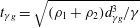$t_{\unicode[STIX]{x1D6FE}g}=\sqrt{(\unicode[STIX]{x1D70C}_{1}+\unicode[STIX]{x1D70C}_{2})d_{\unicode[STIX]{x1D6FE}g}^{3}/\unicode[STIX]{x1D6FE}}$ is the time scale; $d_{\unicode[STIX]{x1D6FE}g}/t_{\unicode[STIX]{x1D6FE}g}$ is the scale for flow velocity; $(\unicode[STIX]{x1D70C}_{1}+\unicode[STIX]{x1D70C}_{2})d_{\unicode[STIX]{x1D6FE}g}^{2}/t_{\unicode[STIX]{x1D6FE}g}^{2}$ is the pressure scale; $qd_{\unicode[STIX]{x1D6FE}g}/(\unicode[STIX]{x1D705}_{1}+\unicode[STIX]{x1D705}_{2})$ is the temperature scale, and $(\unicode[STIX]{x1D70C}_{1}+\unicode[STIX]{x1D70C}_{2})d_{\unicode[STIX]{x1D6FE}g}/t_{\unicode[STIX]{x1D6FE}g}$ is the scale for the phase transition rate.

Our problem is characterized by the relative densities and coefficients of thermal conductivity of the liquid and its vapour,

by their Reynolds, Péclet and Prandtl numbers,

and also by the dimensionless specific heat of phase transition,

For example, the values of the Reynolds, Péclet and Prandtl numbers for water and its vapour, calculated from the data of table 1, are $Re_{1}=1307.1$ , $Re_{2}=18.6$ , $Pe_{1}=2306.7$ , $Pe_{2}=19.6$ , $Pr_{1}=1.7$ and $Pr_{2}=1.05$ , respectively. The relative density and thermal conductivity of water vapour are $\tilde{\unicode[STIX]{x1D70C}}_{2}=6.2\times 10^{-4}$ and $\tilde{\unicode[STIX]{x1D705}}_{2}=3.4\times 10^{-2}$ , respectively. The corresponding values for water in the liquid state are found from the following expressions: $\tilde{\unicode[STIX]{x1D70C}}_{1}=1-\tilde{\unicode[STIX]{x1D70C}}_{2}$ and $\tilde{\unicode[STIX]{x1D705}}_{1}=1-\tilde{\unicode[STIX]{x1D705}}_{2}$ . The dimensionless specific heat of vapour generation is $\unicode[STIX]{x1D6EC}=3.4\times 10^{8}/q\;(\text{W}~\text{m}^{-2})$ , where the heat flux $q$ is measured in $\text{W}~\text{m}^{-2}$ .

The base state is characterized by the vertical gradients of pressure and temperature, $-\tilde{\unicode[STIX]{x1D70C}}_{j}\boldsymbol{e}_{z}/(\tilde{\unicode[STIX]{x1D70C}}_{1}-\tilde{\unicode[STIX]{x1D70C}}_{2})$ and $\boldsymbol{e}_{z}/\tilde{\unicode[STIX]{x1D705}}_{j}$ , where $\boldsymbol{e}_{z}$ is the unit vector of the vertical axis $z$ . In what follows, the gradients of hydrostatic pressure in the phases are taken into account in normal stress balance equation (3.14). There, along with the capillary pressure, they are included in the term proportional to the amplitude of shape perturbations of the surface, $F$ . The base temperature gradients are responsible for the presence of convective terms in the right-hand sides of energy equations (3.6).

The profiles $P_{j}(z)$ , $U_{jz}(z)$ and $\unicode[STIX]{x1D6E9}_{j}(z)$ specify the dependences of pressure, vertical velocity component, and temperature perturbations on the vertical coordinate $z$ , respectively. The relations for these quantities (see Konovalov et al. Reference Konovalov, Lyubimov and Lyubimova2016), which were obtained from the linearized Navier–Stokes equations and also continuity and energy equations for homogeneous incompressible media, are written as

Here, $\unicode[STIX]{x1D714}$ and $k$ are the eigenfrequency and wavenumber of perturbations, respectively.

The following notation is introduced:

Velocity and temperature perturbations are damped in the layers of the liquid and its vapour at $z\rightarrow \pm \infty$ , respectively,

Boundary conditions associated with the liquid–vapour interface are linearized and transported to the coordinate surface $z=0$ . These are conditions (3.10) and (3.11) below, which, when taken together, represent the mass balance of matter in the phases and define the rate of phase transition. Then follow the boundary conditions obtained from continuity of tangential velocity components (3.12), tangential stress continuity (3.13), normal stress balance (3.14), temperature continuity (3.15) and heat flux balance (3.16),

Here, $F$ and $\unicode[STIX]{x1D6EF}$ are the amplitudes of the deviation of the interphase surface from the equilibrium position and rate of phase transition, respectively. The square brackets denote a jump of the corresponding quantities across the interface from the vapour to the liquid.

To close the boundary value problem, it is necessary to prescribe one more boundary condition, which will determine the thermodynamic state of the interface between the phases. Here, we restrict ourselves to its simplest approximate form, assuming that the temperature at the perturbed interface remains equal to the equilibrium saturation temperature $T_{s0}$ ,

This also allows us to ignore thermocapillary forces in condition (3.13). They will be considered in the appendix A of this paper with an emphasis on the weak effect produced by the relationship between the local saturation temperature and media pressure.

It is important to note that the deviation of the interface temperature from the equilibrium temperature occurs due to local temperature perturbations relative to the base state and also due to the displacement of the surface into regions in which the base temperature differs from the base temperature in the initial position. This is reflected in boundary conditions (3.15) and (3.17) containing both the fields $\unicode[STIX]{x1D6E9}_{j}$ and amplitude $F$ .

4 Modification of the problem

Before proceeding to derive an approximation relation for the eigenfrequency shift, we will modify equations (3.4)–(3.6) and boundary conditions (3.8)–(3.17), based on the approach proposed in Cerda & Tirapegui (Reference Cerda and Tirapegui1998), which is generalized here for solving the problem with heat and mass transfer.

General solutions for $U_{jz}$ can be represented in the form of the following sums:

Here, $U_{jz}^{I}$ are particular solutions of equations (3.5) for the corresponding $j$ , and $U_{jz}^{II}$ are general solutions of the homogeneous equations corresponding to (3.5),

or, which is the same,

It is quite possible to assume that each of the solutions $U_{jz}^{I}$ corresponds to a potential viscous flow in an incompressible medium and

Then relations (3.5) for $U_{jz}^{I}$ are reduced to the projections of the Euler equations on the vertical axis $z$ ,

Thus, it is possible not only to separate potential and rotational components of velocity from each other, that, in general, the well-known Helmholtz theorem allows, but also, in the framework of a linearized problem, we can associate the first with pressure perturbations in a unique way.

We write down a series of the transformations of boundary condition (3.13),

associated with the sequential use of expressions (4.1), (4.3) and (4.4) as well as condition (3.10) and its analogue for the vapour (it comes from the replacements $U_{1z}\rightarrow U_{2z}$ and $\tilde{\unicode[STIX]{x1D70C}}_{1}\rightarrow \tilde{\unicode[STIX]{x1D70C}}_{2}$ ). As a result, it reduces to the following form, fulfilled at $z=0$ and free of derivatives with respect to the vertical coordinate $z$ :

Using expressions (4.1) and condition (3.12), boundary condition (3.14), imposed at $z=0$ , can be rewritten as

General solutions for $\unicode[STIX]{x1D6E9}_{j}$ can be represented as the following sums:

Here, $\unicode[STIX]{x1D6E9}_{j}^{I}$ and $\unicode[STIX]{x1D6E9}_{j}^{II}$ are considered to be convective parts of temperature perturbations, which, by virtue of linearity of the problem, are set separately from each other by the corresponding velocity components, $U_{jz}^{I}$ and $U_{jz}^{II}$ , as

It is easy to verify that the sums $\unicode[STIX]{x1D6E9}_{j}^{I}+\unicode[STIX]{x1D6E9}_{j}^{II}$ are particular solutions of inhomogeneous equations (3.6), for this, it is enough to fold the left and right sides of expressions (4.10) and (4.11) and to use expressions (4.1). In turn, $\unicode[STIX]{x1D6E9}_{j}^{III}$ are general solutions of the homogeneous equations corresponding to (3.6),

and hereinafter are called the purely heat-conducting parts of temperature perturbations.

Owing to uniformity of the vertical temperature gradient in the base state, the convective-type perturbations of temperature, $\unicode[STIX]{x1D6E9}_{j}^{I}$ and $\unicode[STIX]{x1D6E9}_{j}^{II}$ , must repeat the dependences of the velocity components $U_{jz}^{I}$ and $U_{jz}^{II}$ on the vertical coordinate $z$ , that means

As a result, from (4.10) and (4.11), the following relations are obtained:

The non-potential flow in the boundary layers creates by convective heat transfer the corresponding thermal inhomogeneity (see (4.15)). It is interesting that, depending on values of the Prandtl number $Pr_{j}=Pe_{j}/Re_{j}$ , the thermal conductivity factor, leading to smoothing of the temperature field, can both weaken and strengthen the solutions of rotational type, $\unicode[STIX]{x1D6E9}_{j}^{II}$ , containing the combinations $Pr_{j}/(Pr_{j}-1)$ , without affecting the potential parts of temperature perturbations, $\unicode[STIX]{x1D6E9}_{j}^{I}$ . This mechanism introduces the viscosities of the phases in the thermal subtask, from which the intensity of the phase transition will be determined below.

By virtue of expressions (4.9), (4.14) and (4.15), boundary conditions (3.15)–(3.17), satisfied at $z=0$ , allow writing in the form that includes both the potential and rotational velocity components, $U_{jz}^{I}$ and $U_{jz}^{II}$ , and heat-conducting parts of temperature perturbations, $\unicode[STIX]{x1D6E9}_{j}^{III}$ , as well as their derivatives in the vertical coordinate $z$ . However, values of $U_{jz}^{I}$ and $\text{d}U_{jz}^{I}/\text{d}z$ can be expressed from the fields $U_{jz}^{II}$ and amplitudes $F$ and $\unicode[STIX]{x1D6EF}$ , using expressions (4.1) and conditions (3.10)–(3.12). The resulting relations

indicate a close relationship of the phase transition amplitude $\unicode[STIX]{x1D6EF}$ with the rotational solutions $U_{jz}^{II}$ and $\unicode[STIX]{x1D6E9}_{j}^{III}$ taken at $z=0$ . The heat flux imbalance at the interphase boundary is created by the process of non-stationary heat transfer in the viscous boundary layers. As was stated in Konovalov et al. (Reference Konovalov, Lyubimov and Lyubimova2017), the heat conduction factor plays an important role here. Indeed, in its absence, if we set $Pe_{j}\rightarrow \infty$ in energy equations (3.6), temperature and velocity perturbations are related as $\unicode[STIX]{x1D6E9}_{j}=\text{i}U_{jz}/\unicode[STIX]{x1D714}\tilde{\unicode[STIX]{x1D705}}_{j}$ . Hence, from conditions of continuity of horizontal velocity component (3.12) and heat flux balance (3.16), it follows that the phase transition rate is $\unicode[STIX]{x1D6EF}=0$ .

The solutions of (3.4), (4.2), (4.5) and (4.12) for perturbations in the liquid, which are damped at $z\rightarrow -\infty$ according to boundary conditions (3.8) and (3.9) and expressions (4.1), (4.9), (4.14) and (4.15), can be written as

For the vapour, it is necessary to use the following solutions, which go to zero at $z\rightarrow \infty$ :

Substituting solutions (4.19)–(4.26) into boundary conditions (3.10)–(3.12), (4.7), (4.8) and (4.16)–(4.18), where, in the first three, expressions (4.1) are applied, we arrive at a system of homogeneous linear algebraic equations for the perturbation amplitudes $a_{1}$ , $a_{2}$ , $a_{3}$ , $b_{1}$ , $b_{2}$ , $b_{3}$ , $F$ and $\unicode[STIX]{x1D6EF}$ :

5 A long-wave correction to the eigenfrequency

In order to obtain necessary estimates from the system of (4.27)–(4.34), it is proposed to divide it into a number of subsystems. The perturbation theory developed below corresponds to the case of a light vapour, weak viscous dissipation in a liquid and its vapour, and same phase transition. The first two requirements are quite obvious, and the last condition is satisfied in the range of heat flux values where the homogeneous model is correct (see (2.2)). This follows from the results of numerical calculations in Konovalov et al. (Reference Konovalov, Lyubimov and Lyubimova2017), considering the similar problem of the Rayleigh–Taylor instability for a configuration of thick layers of phases. Also, we imposed the additional requirement associated with small values of the wavenumber of perturbations.

The eigenfrequency is represented as

Here $\unicode[STIX]{x1D714}_{0}$ is its principal value in the absence of dissipation; $\unicode[STIX]{x0394}\unicode[STIX]{x1D714}_{Re}$ and $\unicode[STIX]{x0394}\unicode[STIX]{x1D714}_{\unicode[STIX]{x1D6EC}}$ are small corrections related to the influence of viscosity and phase transition, respectively.

Next, we introduce a phenomenological coefficient $\unicode[STIX]{x1D6FC}$ expressing the linear amplitude coupling

which is a simple mathematical consequence of the existence of the base state of the system with a flat interphase boundary ( $F=0$ ) without phase transition ( $\unicode[STIX]{x1D6EF}=0$ ). This seems to be convenient if it is possible to separate solutions of the dynamic and thermal subtasks, as for example in the framework of the quasi-equilibrium approximation in Hsieh (Reference Hsieh1978). Generally speaking, the coefficient $\unicode[STIX]{x1D6FC}$ depends on all processes that take place in a perturbed two-layer, two-phase system (see Konovalov et al. Reference Konovalov, Lyubimov and Lyubimova2017), namely the mechanisms of thermal conductivity, convective heat transfer, viscosity and phase transition.

The phase transition through its velocity $\unicode[STIX]{x1D6EF}$ , entering boundary conditions of mass balance (3.10) and (3.11), tends to smooth out the perturbed interface (see Hsieh Reference Hsieh1972, Reference Hsieh1978; Ievlev & Son Reference Ievlev and Son1980), regardless of the viscosities of the liquid and its vapour, which act through the viscous terms in normal stress balance (3.14) and the viscous correction to pressure (see Joseph & Wang Reference Joseph and Wang2004). This allows us to calculate the contribution of the phase transition for a given value of the phenomenological coefficient $\unicode[STIX]{x1D6FC}$ through solving the inviscid problem (see Hsieh Reference Hsieh1978). In doing so, we neglect the secondary effect of redistribution of matter in the phases on the pressure changes produced by viscous flow. According to Adham-Khodaparast et al. (Reference Adham-Khodaparast, Kawaji and Antar1995), it just causes the cut-off wavenumber shift for the Rayleigh–Taylor instability towards the long-wave range, that is controlled in our case by the product of two small quantities, namely the sum of the kinematic viscosities, $Re_{1}^{-1}+Re_{2}^{-1}$ , and the coefficient $\unicode[STIX]{x1D6FC}$ .

Taking into account the remarks of the previous paragraph, we temporarily exclude from consideration the effect of viscosities of the liquid and its vapour, solving the problem of an irrotational flow of inviscid media. The condition that the determinant of system (4.27), (4.28) and (4.31) is equal to zero, taking into account $a_{2}=b_{2}=0$ and $\tilde{\unicode[STIX]{x1D70C}}_{1}+\tilde{\unicode[STIX]{x1D70C}}_{2}=1$ , gives us the dispersion relation

At $\unicode[STIX]{x1D6FC}=0$ , the frequency of undamped waves in the absence of phase transition is found as

Under the condition $\unicode[STIX]{x1D6FC}\ll 1$ , the small contribution of the latter to the eigenfrequency $\unicode[STIX]{x1D714}=\unicode[STIX]{x1D714}_{0}+\unicode[STIX]{x0394}\unicode[STIX]{x1D714}_{\unicode[STIX]{x1D6EC}}$ is

Let us return to consideration of the viscosities of the phases. The value $\unicode[STIX]{x0394}\unicode[STIX]{x1D714}_{Re}$ should be determined from system (4.27)–(4.31) in the absence of phase transition, when, in (4.27), (4.28) and (4.30), the amplitude $\unicode[STIX]{x1D6EF}$ is taken to be zero. Owing to the insignificance of the vapour density, the liquid–vapour interface is practically free. In the limit $\tilde{\unicode[STIX]{x1D70C}}_{2}\rightarrow 0$ and $\tilde{\unicode[STIX]{x1D70C}}_{1}\rightarrow 1$ , this allows us to estimate from (4.27) and (4.30) the amplitudes of velocity perturbations in the liquid as

Equations (4.28) and (4.29), where substitutions (5.6) and (5.7) are made, give the possibility to express the amplitudes of velocity perturbations in the vapour as

These relationships can be simplified by considering $k\ll 1$ , $Re_{2}\gg 1$ and $\sqrt{Re_{1}}\gg \sqrt{Re_{2}}$ . Recall that, for water and its vapour, $Re_{1}=1307.1$ and $Re_{2}=18.6$ . Then

and

Let us substitute expressions (5.9) and (5.10) in (4.27), (4.30) and (4.31), where the following simplifications are applied:

arising from the requirements for the properties of the liquid and its vapour when formulating the problem at the beginning of § 2. As a result, we obtain a system of homogeneous linear algebraic equations for the amplitudes $a_{1}$ , $a_{2}$ and $F$ . The condition that the determinant of this system is zero will lead us to the following dispersion relation (in which the first neglected term was of order $Re_{1}^{-3/2}$ ):

Taking into account the principal eigenfrequency value $\unicode[STIX]{x1D714}_{0}$ (see (5.4)), we obtain its ‘viscous’ correction

This represents in a dimensionless form the result of Dore (Reference Dore1978) (accurate to capillary forces additionally taken into account) for the effects of viscosities of a liquid and gas (vapour) in the absence of phase transformation.

Let us calculate an approximate value of the phenomenological coefficient $\unicode[STIX]{x1D6FC}$ . To do this, we focus on (4.32)–(4.34), in which the viscous solution of the problem expressed by the amplitudes $a_{2}$ and $b_{2}$ is used (see (5.7) and (5.10)). In fact, it should itself depend on the phase transition. In neglecting this, we introduce an error of the second order of smallness in the coefficient $\unicode[STIX]{x1D6FC}$ . We arrive at a system of inhomogeneous linear algebraic equations for the amplitudes $a_{3}$ , $b_{3}$ and $\unicode[STIX]{x1D6EF}$ . Their inhomogeneous parts are proportional to the amplitude $F$ . Solving the system with respect to the amplitude $\unicode[STIX]{x1D6EF}$ , the approximate value of the phenomenological coefficient $\unicode[STIX]{x1D6FC}=-\unicode[STIX]{x1D6EF}/F$ is found as

Here, final expression (5.14) is simplified taking into account that $\tilde{\unicode[STIX]{x1D70C}}_{2}\ll \tilde{\unicode[STIX]{x1D70C}}_{1}\approx 1$ , $\tilde{\unicode[STIX]{x1D705}}_{2}\ll \tilde{\unicode[STIX]{x1D705}}_{1}\approx 1$ , $k\ll 1$ , $Re_{2}\gg 1$ , $\sqrt{Re_{1}}\gg \sqrt{Re_{2}}$ , $Pe_{1}\gg 1$ and $Pe_{2}\gg 1$ (see table 1).

Substituting relation (5.14) into (5.5) gives the following approximation for the correction to the principal eigenfrequency value, $\unicode[STIX]{x1D714}_{0}=\sqrt{k(1+k^{2})}$ , associated with the phase transition:

The quantity $\unicode[STIX]{x0394}\unicode[STIX]{x1D714}_{\unicode[STIX]{x1D6EC}}$ , or rather its real and imaginary parts, monotonically approach saturation in the limit of strong heating,

Estimate (5.16), like the increment due to the vapour viscosity (the second term in expression (5.13)), corresponds to an increase in the damping coefficient of gravity–capillary waves, $\text{Im}\,\unicode[STIX]{x1D714}$ , and equivalent decrease in their real frequency $\text{Re}\,\unicode[STIX]{x1D714}$ . In compliance with (5.16), taking into account $Pe_{2}=Pr_{2}Re_{2}$ , the changes in the wave characteristics caused by the phase transition are limited to the ( $Pr_{2}+\sqrt{Pr_{2}}$ )-th parts of the corresponding contributions of the vapour viscosity.

The part of the dependence $\unicode[STIX]{x0394}\unicode[STIX]{x1D714}_{\unicode[STIX]{x1D6EC}}(\unicode[STIX]{x1D6EC})$ far from the limiting value (5.16) is approximated by the inverse proportionality of the parameter $\unicode[STIX]{x1D6EC}$ , provided that $\unicode[STIX]{x1D6EC}\gg \tilde{\unicode[STIX]{x1D70C}}_{2}^{-1}\sqrt{Pe_{2}/\unicode[STIX]{x1D714}_{0}}$ . This implies an increment to the damping coefficient of perturbations,

at a slight variation in their real frequency. Note that, in contrast with (5.16), this result is more reliable in practice, since it can be approached not running the risk of violating homogeneity criterion (2.2).

6 Numerical results

For numerical verification of the estimates written above, one should return to amplitude system (4.27)–(4.34). It is worthwhile to evaluate its determinant numerically, for example by the method of Gaussian elimination with selection of a leading element. A requirement of equality to zero, applied to the real and imaginary parts of the complex determinant, yields a system of two dispersion relations. Its solutions for the real (real frequency) and imaginary (damping coefficient) parts of the eigenfrequency $\unicode[STIX]{x1D714}$ were also determined numerically by the coordinate descent method with the iteration starting point given by the sum of (5.4), (5.13) and (5.15). The particular cases without heat and mass transfer or vapour viscosity are considered in a similar way through a truncation of system (4.27)–(4.34).

Figure 2.

The real (graphs on the left) and imaginary (graphs on the right) parts of the correction to the eigenfrequency of perturbations due to viscosity as a function of the wavenumber. The graphs are constructed in linear (a,b) and logarithmic (c,d) scales. Solid lines demonstrate numerical data for the general case. Dashed lines show the results of approximation (5.13). Long-dashed lines describe numerical data for the case of inviscid vapour.

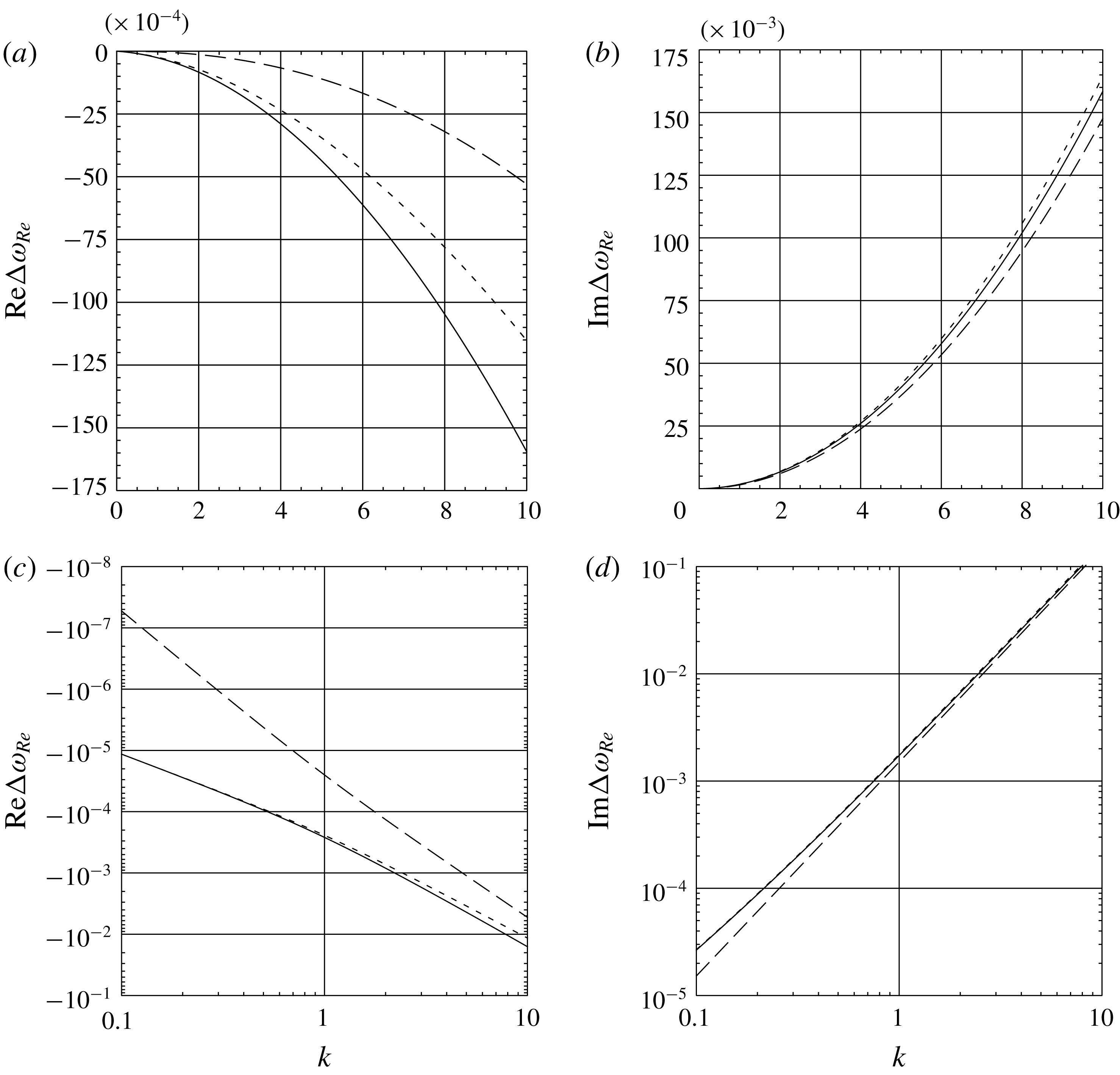
Calculations were carried out on the basis of the data of table 1 in § 2 for water and water vapour. This should be considered as a supplement to the approximate analysis in § 5, which is a generalization of Dore (Reference Dore1978), including capillarity and transfer of matter between the phases. Expression (5.13) (dashed lines in figure 2 a,c) estimates well the imaginary part of the correction $\unicode[STIX]{x0394}\unicode[STIX]{x1D714}_{Re}$ in a wide range of the wavenumber $k$ . Thus, at $k=10$ , the relative error is less than $4\,\%$ and decreases with increasing the perturbation wavelength. As for its real part $\text{Re}\,\unicode[STIX]{x0394}\unicode[STIX]{x1D714}_{Re}$ (see figure 2 a,c), this error already exceeds $7\,\%$ for $k=1$ but is also found to be much smaller in the long-wave range.

Table 2.

Viscous damping in the water–water vapour system.

Table 3.

The effect of phase transition in the water–water vapour system.

In full accordance with the conclusions of Dore (Reference Dore1978), the numerical calculations confirm the importance of considering the viscosity of the light vapour. The corresponding changes in the real and imaginary parts of the correction $\unicode[STIX]{x0394}\unicode[STIX]{x1D714}_{Re}$ as well as those related to the viscosity of the liquid (see solid and long-dashed lines in figure 2 a–d) increase with a growth of the wavenumber $k$ . But, the factor of vapour viscosity becomes of principal importance for sufficiently long waves.

Figure 3.

The imaginary part of the correction to the eigenfrequency of perturbations due to the phase transition as a function of the parameter $\unicode[STIX]{x1D6EC}$ (graphs on (a)) and wavenumber (graphs on (b)). The graphs on the left are plotted for the following values of the wavenumber $k$ : $0.1$ (1), $1$ (2) and $10$ (3). The graphs on the right are plotted for the following values of the parameter $\unicode[STIX]{x1D6EC}$ : $10^{4}$ (1), $10^{6}$ (2) and $10^{8}$ (3). Solid lines demonstrate numerical data. Dashed lines correspond to the results of approximation (5.15). Long-dashed lines describe the numerically calculated contribution of media viscosities, $\text{Im}\unicode[STIX]{x0394}\unicode[STIX]{x1D714}_{Re}$ .

Move on to the effect of phase transition. There is a horizontal asymptote in the graph $\text{Re}\unicode[STIX]{x0394}\unicode[STIX]{x1D714}_{\unicode[STIX]{x1D6EC}}(\unicode[STIX]{x1D6EC})$ in figure 3(a), associated with the upper bound on the intensity of the phase transition (see Konovalov et al. Reference Konovalov, Lyubimov and Lyubimova2016, Reference Konovalov, Lyubimov and Lyubimova2017). A passage to the asymptote begins at $\unicode[STIX]{x1D6EC}\lesssim 10^{3}\,k^{-1}$ (here the contributions of the phase transition and viscosity of the media differ at most by an order of magnitude). It should be emphasized once more that we use the model of homogeneous media, which is in reality correct only at $\unicode[STIX]{x1D6EC}\gg 6\times 10^{5}~\text{k}^{-1}$ (see (2.2)).

Figure 4.

The ratio of the real and imaginary parts of the correction to the eigenfrequency of perturbations due to the phase transition as a function of the parameter $\unicode[STIX]{x1D6EC}$ . The graphs are constructed for the following values of the wavenumber $k$ : $0.1$ (1), $1$ (2) and $10$ (3), based on the results of numerical calculations (solid lines) and approximation (5.15) (dashed lines).

The smaller the wavenumber $k$ is, the closer to each other are the numerical and estimated (see (5.15)) data for the imaginary part of the correction $\unicode[STIX]{x0394}\unicode[STIX]{x1D714}_{\unicode[STIX]{x1D6EC}}$ (compare solid and dashed lines in figure 3 a,b). In general, we can observe a growth of $\text{Im}\unicode[STIX]{x0394}\unicode[STIX]{x1D714}_{\unicode[STIX]{x1D6EC}}$ with increasing $k$ . In figure 4, it is convenient to demonstrate the ratio of the real and imaginary parts, $\text{Re}\unicode[STIX]{x0394}\unicode[STIX]{x1D714}_{\unicode[STIX]{x1D6EC}}/\text{Im}\unicode[STIX]{x0394}\unicode[STIX]{x1D714}_{\unicode[STIX]{x1D6EC}}$ , which is also more accurately described by approximation (5.15) for the case of small $k$ . Note that the denominator $\text{Im}\unicode[STIX]{x0394}\unicode[STIX]{x1D714}_{\unicode[STIX]{x1D6EC}}$ is always positive. However, the quantity $\text{Re}\unicode[STIX]{x0394}\unicode[STIX]{x1D714}_{\unicode[STIX]{x1D6EC}}$ in the numerator can change its sign. By the way, this is not evident from the graphs corresponding to approximation (5.15). Estimate (5.17), which apparently requires smallness of $|\text{Re}\unicode[STIX]{x0394}\unicode[STIX]{x1D714}_{\unicode[STIX]{x1D6EC}}/\text{Im}\unicode[STIX]{x0394}\unicode[STIX]{x1D714}_{\unicode[STIX]{x1D6EC}}|$ , is not always correct.

Tables 2 and 3 represent examples of computations, which comply with possible experimental conditions. From these tables, it is clear that the phase transition as a factor of stability can be easily neglected at least for the interface between thick layers of a liquid and its vapour.