2.1. Governing equations and challenging cases

Consider, as shown in figure 1, a solid and arbitrarily shaped no-slip body $\mathcal P$ (also termed particle) immersed in a Newtonian fluid bounded by a solid, motionless, impermeable and plane slip wall $\varSigma .$

Figure 1.

A solid, arbitrarily shaped and no-slip particle ${\mathcal P},$ with length scale $a,$ immersed in a Newtonian liquid near the $x_3=0$ motionless, impermeable and slipping plane wall $\varSigma .$ The particle–wall gap is $d$ , the wall slip length is $\lambda$ and M designates a point located in the $ x_{3}\gt 0$ domain. The particle is suspended in a prescribed ambient flow $(\boldsymbol {u}_a,p_a)$ and its rigid-body motion has translational velocity $\boldsymbol {U}$ and angular velocity ${\boldsymbol \varOmega }.$ For example, the velocity profile of a ‘linear’ ambient shear flow is drawn for $\lambda \gt 0.$

The particle length scale is $a$ and the wall–particle gap is $d\gt 0.$ Note that this work therefore disregards the case of a particle in contact with the wall.

We use Cartesian coordinates $(O,x_1, x_2, x_3),$ with origin $O$ attached to the $x_3=0$ plane wall $\varSigma$ and associated unit vectors $(\boldsymbol {e}_1, \boldsymbol {e}_2, \boldsymbol {e}_3).$ Thus, a point M located in the $x_{3}\gt 0$ domain (see figure 1) is located with $ \boldsymbol {x}=\boldsymbol{O \kern-2pt M}$ and one has $x_{i}=\boldsymbol {x}\boldsymbol{\cdot }\boldsymbol {e}_{i}.$ The fluid uniform density is $\rho_{\kern-1pt f}$ and its viscosity is $\mu \gt 0.$ Far from the particle a prescribed arbitrary ambient steady Stokes flow, with velocity $\boldsymbol {u}_a$ and pressure $p_a,$ might be imposed. This ambient flow satisfies the Stokes equations together with appropriate boundary conditions on the impermeable slip wall $\varSigma .$ More precisely,

(2.1) \begin{align} \mu {\boldsymbol{\nabla} }^2\boldsymbol {u}_a &={\boldsymbol{\nabla }\!}p_a\,\text{and}\,{\boldsymbol{\nabla }}\boldsymbol{\cdot }\boldsymbol {u}_a=0 \text{ for }{ x_3\gt 0,} \end{align}

(2.2) \begin{align} \boldsymbol {u}_a\boldsymbol{\cdot }\boldsymbol {e} _3 &=0\,\text{and}\,\boldsymbol {u}_a\boldsymbol{\cdot }\boldsymbol {e}_{\!j}=\lambda \left[{{\partial \boldsymbol {u}_a\boldsymbol{\cdot }\boldsymbol {e}_{\!j}}\over {\partial x_3}}\right]\, {\text{for } j=1,2 \text{ on } \varSigma (x_3=0).} \end{align}

As discussed in the introduction, the second condition (2.2) is the Navier (Reference Navier1823) slip condition on the wall with slip length $\lambda \geqslant 0.$ For example, an ambient shear flow with velocity $\boldsymbol {u}_a=[k_l(x_3+\lambda )+k_q x_3^2]\boldsymbol {e}_1$ and pressure $p_a=2\mu k_q x_3$ satisfies (2.1)–(2.2). It has parameters $k_l$ and $k_q$ associated with a ‘linear’ and a quadratic shear flow, respectively.

As shown in figure 1, the particle rigid-body motion has translational velocity $\boldsymbol {U}$ (here the velocity of the point $O'$ attached to the particle) and angular velocity ${\boldsymbol \varOmega }.$ The particle affects the ambient flow so that the flow about the particle has velocity $\boldsymbol {u}_a+\boldsymbol {u}$ and pressure $p_a+p$ in the fluid domain ${\mathcal D}.$ The flow Reynolds number is $ {Re}=\rho_{\kern-1pt f} V a/\mu$ with $a$ the particle length scale and $V$ the typical magnitude of $\boldsymbol {u}_a+\boldsymbol {u}.$ Assuming that $ {Re}\ll 1$ ensures that, like $(\boldsymbol {u}_a,p_a),$ the flow $(\boldsymbol {u},p)$ satisfies the steady Stokes equations. The particle surface $S$ is no-slip and the flow $(\boldsymbol {u},p)$ therefore obeys

(2.3) \begin{align} \mu {\boldsymbol{\nabla} }^2\boldsymbol {u}&={\boldsymbol{\nabla }}p\,\text{and}\,{\boldsymbol{\nabla }}\boldsymbol{\cdot }\boldsymbol {u}=0\quad\text{in }{\mathcal D},\, (\boldsymbol {u},p)\rightarrow (\boldsymbol {0},0)\,\text{as}\,|\boldsymbol{O \kern-2pt M}|\rightarrow \infty , \end{align}

(2.4) \begin{align} \boldsymbol {u}\boldsymbol{\cdot }\boldsymbol {e}_3&=0\,\text{and}\,\boldsymbol {u}\boldsymbol{\cdot }\boldsymbol {e}_{\!j}=\lambda \left[{{\partial \boldsymbol {u}\boldsymbol{\cdot }\boldsymbol {e}_{\!j}}\over {\partial x_3}}\right]\, {\text{for } j=1,2 \text{ on } \varSigma (x_3=0),} \end{align}

(2.5) \begin{align} \boldsymbol {u}&=-\boldsymbol {u}_a+\boldsymbol {U}+{\boldsymbol\varOmega }\wedge \boldsymbol{O}'\!\boldsymbol{M}\,\text{on }S. \end{align}

The flow $(\boldsymbol {u},p)$ has stress tensor ${\boldsymbol \sigma }.$ It exerts on the particle boundary $S,$ having unit normal $\boldsymbol {n}$ pointing into the fluid, a surface stress $\boldsymbol {f}={\boldsymbol \sigma }\boldsymbol{\cdot }\boldsymbol {n}.$ Likewise, the ambient flow field $(\boldsymbol {u}_a,p_a)$ with stress tensor ${{\boldsymbol \sigma }\!}_a$ induces on $S$ a stress $\boldsymbol {f\!}_a={{\boldsymbol \sigma }\!}_a\boldsymbol{\cdot }\boldsymbol {n}.$ Since (2.1) also holds inside the particle, integrating $\boldsymbol {f\!}_a$ and its first moment on $S$ yields zero force and torque on the particle. Accordingly, the force $\boldsymbol {F}$ and the torque $\boldsymbol\varGamma$ (about the point $O')$ exerted by the flow $(\boldsymbol {u}_a+\boldsymbol {u},p_a+p)$ on the particle can be written

(2.6) \begin{equation} \boldsymbol {F}=\int _S {\boldsymbol \sigma }\boldsymbol{\cdot }\boldsymbol {n}{\rm d}S,\,{\boldsymbol\varGamma }=\int _S \boldsymbol{O}'\!\boldsymbol{M}\wedge {\boldsymbol \sigma }\boldsymbol{\cdot }\boldsymbol {n}{\rm d}S. \end{equation}

The problem (2.3)–(2.5) is linear in both the ambient flow $(\boldsymbol {u}_a,p_a)$ and the particle rigid-body motion $(\boldsymbol {U},{\boldsymbol \varOmega }).$ Therefore, it is possible to distinguish three different cases.

Case 1 is for a particle moving with a given rigid-body motion $(\boldsymbol {U},{\boldsymbol \varOmega })$ in a quiescent liquid, i.e. for $(\boldsymbol {u}_a,p_a)=(\boldsymbol {0},0).$ By linearity, the hydrodynamic force $\boldsymbol {F}_{\!h}$ and torque ${\boldsymbol\varGamma }_h$ experienced by the particle are written $\boldsymbol {F}_{\!h}=-\mu \{\boldsymbol {A}\boldsymbol{\cdot }\boldsymbol {U}+\boldsymbol {B}\boldsymbol{\cdot }{\boldsymbol \varOmega }\}$ and ${\boldsymbol\varGamma }_h=-\mu \{\boldsymbol {C}\boldsymbol{\cdot }\boldsymbol {U}+\boldsymbol {D}\boldsymbol{\cdot }{\boldsymbol \varOmega }\}$ with so-called resistance second-rank tensors $\boldsymbol {A}, \boldsymbol {B}, \boldsymbol {C}$ and $\boldsymbol {D}$ depending upon the wall slip length $\lambda$ and the particle geometry and location.

Case 2 is for a particle held fixed $(\boldsymbol {U}={\boldsymbol \varOmega }=\boldsymbol {0})$ in the ambient flow. As shown in § 2.2, both the force $\boldsymbol {F}_{\!a}$ and the torque ${\boldsymbol\varGamma }_a$ exerted on the particle can be obtained by solely solving the previous Case 1.

Case 3 is for a particle freely suspended in the ambient flow. Combining the previous Cases 1 and 2 gives $\boldsymbol {F}=\boldsymbol {F}_{\!h}+\boldsymbol {F}_{\!a}$ and ${\boldsymbol\varGamma }={\boldsymbol\varGamma }_h+{\boldsymbol\varGamma }_a.$ Imposing the freely suspended particle to be force-free and torque-free provides its rigid-body motion $(\boldsymbol {U},{\boldsymbol \varOmega })$ by solving the linear equations $\mu \{\boldsymbol {A}\boldsymbol{\cdot }\boldsymbol {U}+\boldsymbol {B}\boldsymbol{\cdot }{\boldsymbol \varOmega }\}=\boldsymbol {F}_{\!a}$ and $\mu \{\boldsymbol {C}\boldsymbol{\cdot }\boldsymbol {U}+\boldsymbol {D}\boldsymbol{\cdot }{\boldsymbol \varOmega }\}={\boldsymbol\varGamma }_a.$ The stress $\boldsymbol {f\!}_a+\boldsymbol {f}$ on the particle surface $S$ is subsequently obtained in two steps: first, by calculating $\boldsymbol {f\!}_a={{\boldsymbol \sigma }\!}_a\boldsymbol{\cdot }\boldsymbol {n}$ and then getting the flow $(\boldsymbol {u},p)$ solution to (2.3)–(2.5) for the rigid-body motion $(\boldsymbol {U},{\boldsymbol \varOmega })$ to obtain its traction $\boldsymbol {f}={\boldsymbol \sigma } \boldsymbol{\cdot }\boldsymbol {n}$ . This stress $\boldsymbol {f\!}_a+\boldsymbol {f}$ can in practice be obtained by solving a boundary-integral equation (see (3.4)). Once known, it permits one to calculate the second-rank symmetric stresslet tensor $\boldsymbol {S}$ defined as (since the particle is force-free the definition of $\boldsymbol {S}$ is independent of the selected point $O^\prime$ )

(2.7) \begin{equation} \boldsymbol {S}={{1}\over {2}}\int _S\biggl \{\boldsymbol{O}'\!\boldsymbol{M} \otimes (\boldsymbol {f\!}_a+\boldsymbol {f})+ (\boldsymbol {f\!}_a+\boldsymbol {f})\otimes \boldsymbol{O}'\!\boldsymbol{M}-{{2}\over {3}} \big[(\boldsymbol {f\!}_a+\boldsymbol {f})\boldsymbol{\cdot }\boldsymbol{O}'\!\boldsymbol{M} \big]\boldsymbol {I} \biggl \}{\rm d}S \end{equation}

with $\boldsymbol {I}$ the identity tensor. For instance, the component $S_{13}=\boldsymbol {e}_1\boldsymbol{\cdot }\boldsymbol {S}\boldsymbol{\cdot }\boldsymbol {e}_3$ is the essential ingredient in the calculation of the effective viscosity of a dilute suspension of particles subject to ambient ‘linear’ shear flow either for an unbounded suspension (see Batchelor Reference Batchelor1970; Batchelor & Green Reference Batchelor and Green1972a ,Reference Batchelor and Green b ) or, as shown in Tözeren & Skalak (Reference Tözeren and Skalak1983), for a suspension bounded by a no-slip plane wall.

2.2. Extended reciprocal identity and resulting well-posed linear system

This subsection extends for a fluid bounded by the plane slip wall $\varSigma$ the usual material available in standard textbooks (see Happel & Brenner Reference Happel and Brenner1973; Kim & Karrila Reference Kim and Karrila1991) for the unbounded fluid case. Consider two flow fields $(\boldsymbol {u},p)$ and $(\boldsymbol {u}',p')$ obeying (2.3). Let their stress tensors be $\boldsymbol \sigma$ and ${\boldsymbol \sigma }',$ respectively. Mimicking the treatment given in Happel & Brenner (Reference Happel and Brenner1973) for the unbounded fluid, then easily yields

(2.8) \begin{equation} \int _{S\cup \varSigma }[\boldsymbol {u}\boldsymbol{\cdot }{\boldsymbol \sigma }'\boldsymbol{\cdot }\boldsymbol {n}-\boldsymbol {u}'\boldsymbol{\cdot }{\boldsymbol \sigma }\boldsymbol{\cdot }\boldsymbol {n}]{\rm d}S=0,\, \int _{S\cup \varSigma }\boldsymbol {u}\boldsymbol{\cdot }{\boldsymbol \sigma }\boldsymbol{\cdot }\boldsymbol {n}{\rm d}S=-2\mu \int _{{\mathcal D}}e_{\textit{ij}}e_{\textit{ij}}{\rm d}\varOmega \end{equation}

with $\mathcal D$ the liquid domain. In (2.8) there is a summation over indices $i$ and $j$ (taking the values 1, 2, 3) and $e_{\textit{ij}}$ designates the Cartesian component of the flow second-rank rate of strain tensor $\boldsymbol {e}.$ Hence, setting $u_i=\boldsymbol {u}\boldsymbol{\cdot }\boldsymbol {e}_i$ and $u_{i,j}=\partial u_i/\partial x_{\!j}$ gives $e_{\textit{ij}}=(u_{i,j}+u_{j,i})/2.$ Requiring both $\boldsymbol {u}$ and $\boldsymbol {u}'$ to satisfy the Navier boundary conditions (2.4) on the $x_3=0$ slip wall $\varSigma$ also yields (recall, see figure 1, that $\boldsymbol {n}=\boldsymbol {e}_3$ and also that $u_{3,j}=u_3=u^{\prime}_{3,j}=u^{\prime}_3=0$ for $j=1,2$ on $\varSigma $ )

(2.9) \begin{align} \boldsymbol {u}\boldsymbol{\cdot }{\boldsymbol \sigma }'\boldsymbol{\cdot }\boldsymbol {n}&=\lambda \mu \left(u_{1,3}u^{\prime}_{1,3}+u_{2,3}u^{\prime}_{2,3}\right)=\boldsymbol {u}'\boldsymbol{\cdot }{\boldsymbol \sigma }\boldsymbol{\cdot }\boldsymbol {n} \,\text{and} \nonumber\\ \boldsymbol {u}\boldsymbol{\cdot }{\boldsymbol \sigma }'\boldsymbol{\cdot }\boldsymbol {n}&=\lambda \mu \big\{(u_{1,3})^2+(u_{2,3})^2\big\}\, {\text{on } \varSigma .} \end{align}

According to (2.8)–(2.9) two arbitrary flows $(\boldsymbol {u},p)$ and $(\boldsymbol {u}',p')$ fulfilling (2.3)–(2.4) satisfy, whatever the wall slip length $\lambda \geqslant 0,$ the key identities and inequality

(2.10) \begin{align} \int _S\boldsymbol {u}\boldsymbol{\cdot }{\boldsymbol \sigma }'\boldsymbol{\cdot }\boldsymbol {n}{\rm d}S&=\int _S\boldsymbol {u}'\boldsymbol{\cdot }{\boldsymbol \sigma }\boldsymbol{\cdot }\boldsymbol {n}{\rm d}S, \end{align}

(2.11) \begin{align} E_S:= \int _S\boldsymbol {u}\boldsymbol{\cdot }{\boldsymbol \sigma }\boldsymbol{\cdot }\boldsymbol {n}{\rm d}S&=-\mu \left [2\int _{{\mathcal D}}e_{\textit{ij}}e_{\textit{ij}}{\rm d}\varOmega +\lambda \int _{\varSigma }\big\{(u_{1,3})^2+(u_{2,3})^2\big\}{\rm d}S \right ]\lt 0.\\[9pt] \nonumber \end{align}

The result (2.10) is an extension of the Lorentz reciprocity theorem for two arbitrary flows $(\boldsymbol {u},p)$ and $(\boldsymbol {u}',p')$ bounded by the slip wall $\varSigma .$ The equality (2.11) expresses the rate of energy dissipation, $E_S,$ of the surface stress $\boldsymbol {f}={\boldsymbol \sigma }\boldsymbol{\cdot }\boldsymbol {n}$ on the particle boundary $S.$ The inequality $E_S\lt 0$ is valid whatever the wall slip length $\lambda \geqslant 0$ and the flow $(\boldsymbol {u},p)$ obeying (2.3)–(2.4) (of course, we actually discard the quiescent fluid case for which $E_S=0$ ).

In dealing with Case 1 let us introduce for ${i}=1,2,3$ six auxiliary flows $(\boldsymbol {u}^{(i)}_t, p^{(i)}_t)$ and $(\boldsymbol {u}^{(i)}_r, p^{(i)}_r)$ obeying (2.3)–(2.4) and the boundary conditions $\boldsymbol {u}^{(i)}_t=\boldsymbol {e}_i$ and $\boldsymbol {u}^{(i)}_r=\boldsymbol {e}_i\wedge \boldsymbol{O}'\!\boldsymbol{M}$ on the particle surface $S.$ These flows are induced by a translation or a rotation of the particle in quiescent fluid. For $L=t,r$ the flow $(\boldsymbol {u}^{(i)}_L, p^{(i)}_L)$ has stress tensor ${\boldsymbol \sigma }^{(i)}_L$ and exerts on $S$ a stress $\boldsymbol {f}^{(i)}_L={\boldsymbol \sigma }^{(i)}_L\boldsymbol{\cdot }\boldsymbol {n}.$ The Cartesian components $A_{\textit{ij}}, B_{\textit{ij}}, C_{\textit{ij}}$ and $D_{\textit{ij}}$ of the resistance tensors $\boldsymbol {A}, \boldsymbol {B}, \boldsymbol {C}$ and $\boldsymbol {D}$ introduced in § 2.1 are then expressed as

(2.12) \begin{align} A_{\textit{ij}}&=-{\frac {1}{\mu }}\left[\int _S\boldsymbol {e}_i\boldsymbol{\cdot }\boldsymbol {f}^{(j)}_t {\rm d}S\right]\!,\, B_{\textit{ij}}=-{\frac {1}{\mu }}\left[\int _S\boldsymbol {e}_i\boldsymbol{\cdot }\boldsymbol {f}^{(j)}_r {\rm d}S\right]\!, \end{align}

(2.13) \begin{align} C_{\textit{ij}}&=-{\frac {1}{\mu }}\left[\int _S\boldsymbol {e}_i\boldsymbol{\cdot }\left(\boldsymbol{O}'\!\boldsymbol{M}\wedge \boldsymbol {f}^{(j)}_t\right){\rm d}S\right]\!,\, D_{\textit{ij}}=-{\frac {1}{\mu }}\left[\int _S\boldsymbol {e}_i\boldsymbol{\cdot }\left(\boldsymbol{O}'\!\boldsymbol{M}\wedge \boldsymbol {f}^{(j)}_r\right){\rm d}S\right]\!. \end{align}

In Case 2, the particle held fixed in the ambient flow $(\boldsymbol {u}_a,p_a)$ experiences a force $\boldsymbol {F}_{\!a}$ and a torque ${\boldsymbol\varGamma }_a.$ These vectors are obtained by applying the reciprocal identity (2.10) to the perturbed flow $(\boldsymbol {u},p)$ about the fixed particle and the flows $(\boldsymbol {u}^{(i)}_L, p^{(i)}_L).$ Adopting henceforth the usual summation convention over repeated indices then gives

(2.14) \begin{equation} \boldsymbol {F}_{\!a}=-\left[\int _S\boldsymbol {u}_a\boldsymbol{\cdot }\boldsymbol {f}^{(i)}_t {\rm d}S\right]\boldsymbol {e}_i,\, {\boldsymbol\varGamma }_a=-\left[\int _S\boldsymbol {u}_a\boldsymbol{\cdot }\boldsymbol {f}^{(i)}_r {\rm d}S\right]\boldsymbol {e}_i. \end{equation}

Accordingly, the Cartesian components $\boldsymbol {U}=U_{\!j}\boldsymbol {e}_{\!j}$ and ${\boldsymbol \varOmega }=\varOmega _{\!j}\boldsymbol {e}_{\!j}$ of the freely suspended particle translational and angular velocities satisfy for $i=1,2,3$ the equations

(2.15) \begin{equation} \mu \big\{A_{\textit{ij}}U_{\!j}+B_{\textit{ij}}\varOmega _{\!j} \big\}=\int _S\boldsymbol {u}_a.\boldsymbol {f}^{(i)}_t {\rm d}S,\, \mu \big\{C_{\textit{ij}}U_{\!j}+D_{\textit{ij}}\varOmega _{\!j} \big\}=\int _S\boldsymbol {u}_a.\boldsymbol {f}^{(i)}_r {\rm d}S. \end{equation}

The linear system (2.15) is written $\boldsymbol {R}\boldsymbol{\cdot }{(}^t\!\boldsymbol{X}{)}=\boldsymbol {Y}$ with $^t\!\boldsymbol{X}$ the transpose of $\boldsymbol {X}=(\boldsymbol {U},{\boldsymbol \varOmega })$ and $\boldsymbol {R}$ the so-called $6\times 6$ resistance matrix. Applying (2.12)–(2.13) and the reciprocal identity (2.10) gives $A_{\textit{ij}}=A_{ji},\ B_{\textit{ij}}=C_{ji}$ and $D_{\textit{ij}}=D_{ji}$ so that $\boldsymbol {R}$ is symmetric. Moreover, from (2.11) one gets $E_S=-\mu \boldsymbol {X}\boldsymbol{\cdot }\boldsymbol {R}\boldsymbol{\cdot }{(}^t\!\boldsymbol{X}{)}\lt 0$ whatever the non-zero particle rigid-body motion $\boldsymbol {X}.$ Thus, $\boldsymbol {R}$ is positive-definite. Consequently, the linear system (2.15) has a unique solution $(\boldsymbol {U},{\boldsymbol \varOmega }).$

3.1. Boundary-integral approach

The flow $(\boldsymbol {u},p),$ solution to (2.3)–(2.5), is obtained by a boundary-integral method. This is done by extending the material presented for a no-slip wall in Pozrikidis (Reference Pozrikidis1992). The main results are given while, since elementary, the proofs are left to the reader.

Consider for $j=1,2,3$ the fundamental Stokes flow produced, above the slip wall and in the absence of the particle, by a force with strength $\boldsymbol {e}_{\!j}$ concentrated at a source point $\boldsymbol {y}$ located in the $y_3\gt 0$ domain. The flow velocity $\boldsymbol {v}^{(j)}(\boldsymbol {x},\boldsymbol {y})$ and pressure $p^{(j)}(\boldsymbol {x},\boldsymbol {y})$ at any point $\boldsymbol {x}$ above the wall $(x_3\geqslant 0)$ satisfy

(3.1) \begin{align} \mu {\boldsymbol{\nabla} }^2\boldsymbol {v}^{(j)}&={\boldsymbol{\nabla }}p^{(k)}-\delta _{3d}(\boldsymbol {x}-\boldsymbol {y})\boldsymbol {e}_k,\!\!\quad\! {\boldsymbol{\nabla }}\boldsymbol{\cdot }\boldsymbol {v}^{(j)}=0,\!\!\quad \big(\boldsymbol {u}^{(j)},p^{(j)}\big)\rightarrow (\boldsymbol {0},0)\!\!\!\quad\text{as }|\boldsymbol{O \kern-2pt M}|\rightarrow \infty , \end{align}

(3.2) \begin{align} \boldsymbol {v}^{(j)}\boldsymbol{\cdot }\boldsymbol {e}_3&=0\,{\text {and}}\,\boldsymbol {v}^{(j)}\boldsymbol{\cdot }\boldsymbol {e}_i= \lambda \left[{{\partial \boldsymbol {v}^{(j)}\boldsymbol{\cdot }\boldsymbol {e}_i}\over {\partial x_3}}\right]\, {\text{for } i=1,2 \text{ on } \varSigma (x_3=0),} \end{align}

with $\delta _{3d}(\boldsymbol {x}-\boldsymbol {y})=\delta _d(x_1-y_1)\delta _d(x_2-y_2)\delta _d(x_3-y_3)$ and $\delta _d$ the Dirac distribution. Solving (3.1)–(3.2) provides the second-rank velocity tensor $\boldsymbol {G}(\boldsymbol {x},\boldsymbol {y})$ with Cartesian components $G_{\textit{ij}}(\boldsymbol {x},\boldsymbol {y})=8\pi \mu \boldsymbol {v}^{(j)}(\boldsymbol {x},\boldsymbol {y})\boldsymbol{\cdot }\boldsymbol {e}_i.$ Proceeding as in Pozrikidis (Reference Pozrikidis1992) and using again the reciprocal identity (2.10) yields the symmetry property $G_{\textit{ij}}(\boldsymbol {x},\boldsymbol {y})=G_{ji}(\boldsymbol {y},\boldsymbol {x})$ and a single-layer integral representation, over the particle surface $S$ and in the entire fluid domain ${\mathcal D},$ for each velocity component $u_{\!j}=\boldsymbol {u}\boldsymbol{\cdot }\boldsymbol {e}_{\!j}$ of the flow $(\boldsymbol {u},p)$ solution to (2.3)–(2.5). It reads (summing over indices $i$ in (3.3))

(3.3) \begin{equation} u_{\!j}(\boldsymbol {x})=-{{1}\over {8\pi \mu }}\int _S G_{ji}(\boldsymbol {x},\boldsymbol {y})[\boldsymbol {f\!}_a+\boldsymbol {f}](\boldsymbol {y})\boldsymbol{\cdot }\boldsymbol {e}_i{\rm d}S\, {\text{for}\, \boldsymbol {x}\in {\mathcal D}\, \text{and}\, j=1,2,3.} \end{equation}

For (3.3) recall that $\boldsymbol {f\!}_a$ and $\boldsymbol {f}$ are the surface stresses induced on $S$ by the ambient flow $(\boldsymbol {u}_a,p_a)$ and the perturbation flow $(\boldsymbol {u},p).$ Actually, (3.3) still holds as $\boldsymbol {x}$ tends onto $S.$ Imposing (2.5) then yields the following boundary-integral equation:

(3.4) \begin{equation} 8\pi \mu \big[\boldsymbol {u}_a(\boldsymbol {x})-\boldsymbol {U}-{\boldsymbol\varOmega }\wedge \boldsymbol{O}'\!\boldsymbol{M} \big]= \int _S \boldsymbol {G}(\boldsymbol {x},\boldsymbol {y})\boldsymbol{\cdot }[\boldsymbol {f\!}_a+\boldsymbol {f}](\boldsymbol {y}){\rm d}S\, {\text{for } \boldsymbol {x} \text{ on } S} \end{equation}

for the stress $\boldsymbol {f\!}_a+\boldsymbol {f}$ exerted on the particle boundary.

The boundary-integral equation (3.4) is of the first kind. Usually, integral equations of the first kind can be ill-posed. Here, the solution $\boldsymbol {f\!}_a +\boldsymbol {f}$ to (3.4) is defined up to a constant multiple of $\boldsymbol {n}$ which, however, does not affect the resistance matrix Cartesian components (2.12)–(2.13) and the force $\boldsymbol {F}_{\!a}$ and torque ${\boldsymbol\varGamma }_a$ given by (2.14). Despite this property, Youngren & Acrivos (Reference Youngren and Acrivos1975) found for an unbounded fluid that the numerical treatment of (3.4) provides accurate solutions and stated that ‘very accurate solutions were obtained with minimal difficulty, a fact which suggests that any ill-conditioning that may exist is much less serious for this particular equation than for other integral equations of the first kind’. The same nice behaviour has been observed in the present work for (3.4). As detailed in § 4.2, accurate results have been obtained nicely agreeing with the literature which resorts to quite different approaches. In this work the particle surface $S$ is meshed using six-node curved boundary elements and this enables us to accurately invert (3.4) spreading on $S$ a reasonable number of nodal points and therefore ending up with a well-conditioned matrix for the linear system resulting from discretising (3.4). It is also theoretically possible to start from a velocity integral representation different from (3.3) and termed compound double-layer representation (see Pozrikidis Reference Pozrikidis1992). This approach, pioneered in Power & Miranda (Reference Power and Miranda1987), ends up with a well-posed boundary-integral equation of the second kind replacing (3.4). Unfortunately, it requires calculation of the third-rank stress tensor $\boldsymbol {T}$ associated with the problem second-rank Green velocity tensor G given in § 3.2. Since the determination of $\boldsymbol {T}$ is very cumbersome, such a procedure is not worked out in this work.

From the (numerical) knowledge of the stress $\boldsymbol {f\!}_a+\boldsymbol {f}$ it is possible to subsequently compute in the fluid domain $\mathcal D$ the flow velocity u by implementing the integral representation (3.3). Similarly, the pressure $p$ associated with u also admits a useful integral representation in the fluid domain. This representation requires the determination of the fundamental pressure $p^{(k)}$ for the problem (3.1)–(3.2) and is not provided here.

All Cases 1–3 presented in § 1.2 are solved using (3.4). First, the surface stresses $\boldsymbol {f}^{(i)}_t$ and $\boldsymbol {f}^{(i)}_r$ are obtained by inverting (3.4) for $\boldsymbol {u}_a=\boldsymbol {0}.$ Then, the resistance tensors $\boldsymbol {A}, \boldsymbol {B}, \boldsymbol {C}$ and $\boldsymbol {D}$ follow from (2.11)–(2.12) and $(\boldsymbol {F}_{\!a},{\boldsymbol\varGamma }_a)$ for Case 2 is deduced from (2.14). The linear system (2.15) is solved to get the freely suspended particle rigid-body motion $(\boldsymbol {U},{\boldsymbol \varOmega }).$ Finally, inverting (3.4) provides the stress $\boldsymbol {f\!}_a+\boldsymbol {f}$ and thereby the components of the stresslet tensor defined by (2.7).

3.2. Green tensor

The Green tensor $\boldsymbol {G}$ was obtained in different forms in Lauga & Squires (Reference Lauga and Squires2005) and Elasmi (Reference Elasmi2008). However, these forms are not convenient for a numerical purpose and this perhaps explains why Lauga & Squires (Reference Lauga and Squires2005) did not perform any computation of $\boldsymbol {G}$ . Here, $\boldsymbol {G}$ is thus provided in another closed form which is quite appropriate for an efficient numerical treatment.

In the absence of a wall, $\boldsymbol {G}$ is the free-space Stokeslet tensor $ \boldsymbol {G}^{st}$ given by Lorentz (Reference Lorentz1907). It reads

(3.5) \begin{equation} \boldsymbol {G}^{st}(\boldsymbol {x},\boldsymbol {y})=\boldsymbol {I}/|\boldsymbol {x}-\boldsymbol {y}|+ (\boldsymbol {x}-\boldsymbol {y})\otimes (\boldsymbol {x}-\boldsymbol {y})/|\boldsymbol {x}-\boldsymbol {y}|^3 \end{equation}

with $\boldsymbol {I}=\boldsymbol {e}_i\otimes \boldsymbol {e}_i$ the usual unit tensor. Following the approach of Blake (Reference Blake1971) for the no-slip wall case, $\boldsymbol {G}$ is sought as $\boldsymbol {G}(\boldsymbol {x},\boldsymbol {y})=\boldsymbol {G}^{st}(\boldsymbol {x},\boldsymbol {y}) -\boldsymbol {G}^{st}(\boldsymbol {x},\boldsymbol {y}')+\boldsymbol {W}(\boldsymbol {x},\boldsymbol {y})$ , where $\boldsymbol {y}'$ denotes the symmetric (image point) of $\boldsymbol {y}$ with respect to the slip wall $\varSigma$ at $x_3=0.$ The tensor $\boldsymbol {W},$ which is regular in the entire domain above the wall, is obtained by applying a two-dimensional Fourier transform on the variables $x_1-y_1$ and $x_2-y_2.$ Such a technique has been also worked out in Sellier & Ghalya (Reference Sellier and Ghalya2011) for the more complex case of anisotropic Navier slip on a plane wall. Here, the Cartesian components $W_{\textit{ij}}(\boldsymbol {x},\boldsymbol {y})$ are expressed in terms of seven one-dimensional Hankel integrals. The results are $(\text{taking}\, i=1,2)$

(3.6) \begin{align} W_{i3}(\boldsymbol {x},\boldsymbol {y})&={{2y_3(x_i-y_i)}\over {\rho }} \left[L_1^{1,1}-x_3L_1^{2,1}\right];\quad W_{33}(\boldsymbol {x},\boldsymbol {y})=-2x_3 y_3 L_1^{2,0}, \end{align}

(3.7) \begin{align} W_{11}(\boldsymbol {x},\boldsymbol {y})&=2[x_3 y_3+2\lambda (x_3+y_3)] \biggl \{\left({{x_1-y_1}\over {\rho }}\right)^2 L_1^{2,2}-{{L_1^{1,1}}\over {\rho }}\biggr \}\nonumber \\ &\quad +4\lambda ^2\biggl \{{{L_2^{1,1}}\over {\rho }} -\left({{x_2-y_2}\over {\rho }}\right)^2 L_2^{2,2}\biggr \}+4\lambda L_1^{1,0}, \end{align}

(3.8) \begin{align} W_{21}(\boldsymbol {x},\boldsymbol {y})&={{2(x_1-y_1)(x_2-y_2)}\over {\rho ^2}} \Big \{[x_3 y_3+2\lambda (x_3+y_3)]L_1^{2,2}+ 4\lambda ^2 L_2^{2,2}\Big \}, \end{align}

(3.9) \begin{align} W_{31}(\boldsymbol {x},\boldsymbol {y})&={{2(x_1-y_1)}\over {\rho }} \biggl \{x_3(y_3+2\lambda )L_1^{2,1} +{{\rho y_3}\over {\big(\rho ^2+R_3^{\prime 2}\big)^{3/2}}}\biggr \} \end{align}

with $R^{\prime}_3=x_3+y_3,\ \rho =\{(x_1-y_1)^2+(x_2-y_2)^2\}^{1/2}$ and Hankel integrals $L_1^{p,q}$ and $L_2^{p,q}$ defined in terms of $(\rho ,R^{\prime}_3;\lambda )$ in Appendix A. Moreover, $W_{12}=W_{21}$ while $W_{22}$ and $W_{32}$ are obtained therefrom by switching $x_1-y_1$ and $x_2-y_2$ in (3.7) and (3.9), respectively. For $\lambda =0$ each of the above Hankel integrals can be analytically obtained and one retrieves the Blake (Reference Blake1971) tensor derived for a no-slip plane wall. As $\rho \rightarrow 0$ , each above quantity ${W}_{\!\textit{ij}}(\boldsymbol {x},\boldsymbol {y})$ tends to a finite value given in Appendix A.

3.3. Resulting asymptotic results

For a particle–wall gap $d$ (see figure 1) that is large compared with the wall slip length $\lambda ,$ one expects to retrieve, at leading order, the case of the particle interacting with a no-slip wall located at $x_3={-\lambda }.$ Obtaining a more refined approximation, versus the small parameter $\epsilon =\lambda /d,$ requires additional effort. This can be done, within the previous boundary-integral formulation, by asymptotically expanding the Green tensor $\boldsymbol {G}(\boldsymbol {x},\boldsymbol {y})$ for points $\boldsymbol {x}$ and $\boldsymbol {y}$ located on the particle surface using the property $\text{Min}(x_3,y_3)\geqslant d\gg \lambda .$ Note that in addition to the lengths $d$ and $\lambda ,$ the particle length scale $a$ also arises in the problem.

For a particle that is distant from the slip wall, in the sense $d\gg a$ and $\lambda \leqslant O(a),$ it is possible to use the asymptotic results derived in Khabthani, Sellier & Feuillebois (Reference Khabthani, Sellier and Feuillebois2013) for a particle distant from a porous slab with thickness $e,$ permeability $K\gt 0$ and upper and lower plane surfaces on which Beavers & Joseph (Reference Beavers and Joseph1967) boundary conditions with slip length $\lambda$ apply. The associated Green tensor, obtained in Khabthani et al. (Reference Khabthani, Sellier, Elasmi and Feuillebois2012), is complicated and depends upon $(\sqrt {K}, e, \lambda ).$ It reduces to the present Green tensor $\boldsymbol {G}$ for vanishing $\sqrt {K}.$ Denoting by $\boldsymbol {G}^{\textit{ns}}$ the Blake (Reference Blake1971) Green tensor for a no-slip wall $\varSigma$ at $x_3=0$ (i.e. obtained by taking $\lambda =0$ in § 3.2) and letting $\sqrt {K}$ vanish in (35)–(36) from Khabthani et al. (Reference Khabthani, Sellier and Feuillebois2013) easily yields

(3.10) \begin{equation} \boldsymbol {G}(\boldsymbol {x},\boldsymbol {y})=\boldsymbol {G}^{\textit{ns}}(\boldsymbol {x},\boldsymbol {y})\big[1+O\big(a^2/d^2\big)\big]\quad {\text{for } \boldsymbol {x} \text{ and } \boldsymbol {y} \text{ on } S \text{ and } 0\leqslant \lambda \leqslant O(a)\ll d.} \end{equation}

As worked out in Khabthani et al. (Reference Khabthani, Sellier and Feuillebois2013) for a distant sphere, (3.10) can be used to derive an asymptotic solution of (3.4) for a distant and arbitrary-shaped particle. However, (3.10) only holds for $d\gg O(a)$ although the case $d\leqslant O(a)$ can also occur when $\lambda \leqslant O(a)\ll d.$ The case $\lambda \ll d$ has been treated by Lecoq et al. (Reference Lecoq, Anthore, Cichocki, Szymczak and Feuillebois2004) at the first order in $\epsilon =\lambda /\text{Min}(a,d)\ll 1$ and only for a sphere translating normal to the plane slip wall. The drag experienced by the sphere for the slip wall with sphere–wall gap $d$ is shown by those authors to be, at $O \big(\epsilon ^2 \big),$ the same as for a no-slip wall with sphere–wall gap $d+\lambda .$ Another approach is developed here to extend these results to non-spherical particles and/or other rigid-body motions. It consists of expanding for points $\boldsymbol {x}$ and $\boldsymbol {y}$ on the particle surface $S$ the Green tensor $\boldsymbol {G}(\boldsymbol {x},\boldsymbol {y})$ given in § 3.2 for $\epsilon =\lambda /d\ll 1.$

Indeed, introducing shifted points $\boldsymbol{\tilde {x}}=\boldsymbol {x}+\lambda \boldsymbol {e}_3$ and $\boldsymbol{\tilde {y}}=\boldsymbol {y}+\lambda \boldsymbol {e}_3$ shown in figure 2 and noting that $x_3\geqslant d\gg \lambda$ and $y_3\geqslant d\gg \lambda$ , it is found (see e.g. Appendix B for the component $G_{31})$ that

(3.11) \begin{equation} \boldsymbol {G}(\boldsymbol {x},\boldsymbol {y})=\boldsymbol {G}^{\textit{ns}}(\boldsymbol{\tilde {x}},\boldsymbol{\tilde {y}})\big[1+O \big(\epsilon ^2 \big)\big]\quad {\text{for } \boldsymbol {x} \text{ and } \boldsymbol {y} \text{ on } S \text{ and } \epsilon =\lambda /d\ll 1.} \end{equation}

In contrast to (3.10), the expansion (3.11) brings no restriction on the normalised particle distance $d/a$ from the slip wall and no restriction on the normalised wall slip length $\lambda /a.$ Clearly, the tensor $\boldsymbol {G}^{\textit{ns}}(\boldsymbol{\tilde {x}},\boldsymbol{\tilde {y}})$ is that for a particle interacting with a no-slip wall $\varSigma$ that is shifted normally to the actual wall so that the new particle–wall gap is ${\tilde d}=d+\lambda .$ The different cases associated with $\boldsymbol {G}(\boldsymbol {x},\boldsymbol {y})$ and $\boldsymbol {G}^{\textit{ns}}(\boldsymbol{\tilde {x}},\boldsymbol{\tilde {y}})$ are sketched in figure 2.

Figure 2.

The same particle interacting with a plane wall in two different circumstances. (a) Case of a wall–particle gap $d$ and a slip wall $\varSigma$ with slip length $\lambda \ll d.$ (b) Case of wall–particle gap ${\tilde d}=d+\lambda$ and a no-slip wall. For this figure, $d$ is of the same order as the particle length scale $a.$

At a point $M$ on the particle surface $S$ the key auxiliary stress $\boldsymbol {f}^{(i)}_L$ depends upon $S,$ the wall–particle gap $d,$ the wall slip length $\lambda$ and the location $\boldsymbol {x}'=\boldsymbol{O}'\!\boldsymbol{M}.$ Given a particle and omitting the dependence on $S,$ we note $\boldsymbol {f}^{(i)}_L(\boldsymbol {x}';d,\lambda )$ for the previous stress and $\boldsymbol {R}(d,\lambda )$ for the resulting resistance matrix introduced in § 2.2. Using (3.11) and asymptotically inverting for $\boldsymbol {u}_a=\boldsymbol {0}$ the boundary-integral equation (3.4), versus $\epsilon =\lambda /d\ll 1,$ then yields

(3.12) \begin{align} \boldsymbol {f}^{(i)}_L(\boldsymbol {x}';d,\lambda )=\boldsymbol {f}^{(i)}_L(\boldsymbol {x}';d+\lambda ,0)\big[1+O \big(\epsilon ^2 \big)\big], \!\!\quad\boldsymbol {R}(d,\lambda )=\boldsymbol {R}(d+\lambda ,0)\big[1+O \big(\epsilon ^2 \big)\big]. \\[-20pt] \nonumber \end{align}

The results (3.12), extending those of Lecoq et al. (Reference Lecoq, Anthore, Cichocki, Szymczak and Feuillebois2004) to any rigid-body motion of a particle with arbitrary shape, provide a ‘recipe’ for $\epsilon =\lambda /d\ll 1$ : one can, at $O \big(\epsilon ^2 \big),$ replace the slip wall located at $d$ from the particle with a no-slip wall located at $d+\lambda .$ Clearly, this ‘recipe’ also holds for the settling motion of the particle under a given gravity field in the absence of ambient flow. In contrast, the ‘recipe’ is not always valid for a particle freely suspended in a given ambient flow. This feature is illustrated by considering two examples of ambient shear flows.

(i) Ambient ‘unit linear’ shear flow with velocity ${\boldsymbol{\tilde u}}_a^l=(x_3+\lambda )\boldsymbol {e}_1.$ For this flow the particle experiences a force ${\boldsymbol{\tilde F}}_a^l(d,\lambda )$ and a torque ${\boldsymbol{\tilde \varGamma }}_a^l(d,\lambda )$ when it is held fixed and translational velocity ${\tilde U}^l(d,\lambda )$ and angular velocity $\tilde {\boldsymbol \varOmega }^l(d,\lambda )$ when it is freely suspended. As sketched in figure 2, for figure 2(a) the slip wall is located at a distance $d$ from the particle and for figure 2(b) the wall is no-slip and located at a distance $d+\lambda$ . For each case (2.14) is applied. Noting that in figure 2(b) the ambient velocity is ${\tilde x}_3\boldsymbol {e}_1$ with ${\tilde x}_3=x_3+\lambda$ and recalling (3.12) immediately gives

(3.13) \begin{equation} {\boldsymbol{\tilde V}}^l(d,\lambda )={\boldsymbol{\tilde V}}^l(d+\lambda ,0)\big[1+O \big(\epsilon ^2 \big)\big],\quad {\boldsymbol{\tilde V}}={\boldsymbol{\tilde F}}_a, {\boldsymbol{\tilde \varGamma }}_a, {\boldsymbol{\tilde U}}, \tilde {{\boldsymbol \varOmega }}. \end{equation}

Thus, the ‘recipe’ is valid for the ambient ‘linear’ shear flow.

(ii) Ambient ‘unit’ quadratic shear flow with velocity ${\tilde u}_a^l=x_3^2\boldsymbol {e}_1.$ Here, the notations for the force, torque and velocities are the same as before with the superscript $l$ replaced with $q.$ For the case of figure 2(b) note that on the particle surface $x_3\geqslant d\gg \lambda$ so that ${\tilde x}_3^2\sim x_3^2+2\lambda {\tilde x}_3.$ Consequently,

(3.14) \begin{equation} {\boldsymbol{\tilde V}}^q(d,\lambda )=\big[{\boldsymbol{\tilde V}}^q-2\lambda {\boldsymbol{\tilde V}}^l\big](d+\lambda ,0)\big[1+O \big(\epsilon ^2 \big)\big],\quad {\boldsymbol{\tilde V}}={\boldsymbol{\tilde F}}_a, {\boldsymbol{\tilde \varGamma }}_a, {\boldsymbol{\tilde U}}, \tilde {{\boldsymbol \varOmega }}. \end{equation}

According to (3.14) the ‘recipe’ is not valid for the ambient quadratic shear flow.

4.1. Considered ellipsoidal particles and resulting normalised quantities

Consider, as shown in figure 3(a), a solid ellipsoid with planes of symmetry intersecting at its centre of volume $O',$ normal to the unit vectors ${\tilde {\boldsymbol {e}}}_1, {\tilde {\boldsymbol {e}}}_2$ and ${\tilde {\boldsymbol {e}}}_3$ ; we take $ {\tilde {\boldsymbol {e}}}_2=\boldsymbol {e}_2$ in all examples. The ellipsoid Euler angle of orientation is $\beta ,$ with ${\tilde {\boldsymbol {e}}}_3\boldsymbol{\cdot }\boldsymbol {e}_3=\cos \beta ,$ and its semi-axis in the $(O',{\tilde {\boldsymbol {e}}}_i)$ direction is ${\tilde a}_i$ with ${\tilde a}_1=a, {\tilde a}_2=a/s$ and ${\tilde a}_3=sa$ , where $s\gt 0$ is the shape parameter. The ellipsoid $(s \neq 1)$ has the same volume as a sphere $(s=1)$ with radius $a$ but a surface area ${\mathcal A}_s=4\pi a^2 A_s$ different from the sphere surface area $4\pi a^2.$ Note that $A_s$ is expressed in terms of elliptic integrals (see Bowman Reference Bowman1961) but can also be approximated, with about 1 % relative accuracy, by a simple formula. (As suggested by Knud Thomsen, here $A_s\sim [(s^{-\alpha }+1+s^{\alpha })/3]^{1/\alpha }$ with $\alpha =1.6075.$ ) The ellipsoid centre of volume is $O'$ with $\ell =\boldsymbol {OO'}\boldsymbol{\cdot }\boldsymbol {e}_3.$ A calculus exercise shows that the ellipsoid–wall gap is $d=\ell -a(s^2\cos ^2\beta +\sin ^2\beta )^{1/2}.$

Figure 3.

Considered ellipsoidal and spherical particles interacting with a plane slip wall $\varSigma$ located at the same distance $d$ from the particle surface. (a) Sketch of the $s=2$ inclined ellipsoid with orientation $\beta$ for $0\lt \beta \lt \pi /2.$ (b) Same ellipsoid with orientation $\beta =0.$ (c) Same ellipsoid with orientation $\beta =\pi /2.$ (d) Sphere with radius $a.$ Recall that all particles have the same volume (the ellipsoid semi-axis in the direction $\boldsymbol {e}_2,$ normal to the plane of the figure, is $a/s).$ Bottom row: graphical illustration of the hydrodynamic coefficients introduced by (4.1)–(4.2): (e) $\boldsymbol {U}=U\boldsymbol {e}_1,\ \boldsymbol{\varOmega }=\boldsymbol {0},\ \boldsymbol {F}_{\!h}=6\pi \mu aU\overline {\boldsymbol {F}}_h$ and ${{\varGamma }}_h=8\pi \mu a^2 U\overline { \varGamma }_h$ ; (f) same as (e) with $\boldsymbol {U}=U\boldsymbol {e}_3$ ; (g) ${\boldsymbol \varOmega }=\varOmega \boldsymbol {e}_2,\ \boldsymbol {U}=\boldsymbol {0},\ \boldsymbol {F}_{\!h}=6\pi \mu a^2\varOmega \overline {\boldsymbol {F}}_h$ and ${\varGamma }_h=8\pi \mu a^3\varOmega \overline {\varGamma }_h$ .

For the considered ellipsoids and ambient ‘linear’ or quadratic shear flows the symmetries permit one to restrict attention to $\beta$ in $[0,\pi /2].$ When freely suspended in such ambient flows the ellipsoid rotates about the $(O',\boldsymbol {e}_2)$ axis and translates normal to $\boldsymbol {e}_2.$ Thus, only rigid-body motions $(\boldsymbol {U},{\boldsymbol \varOmega })$ with $\boldsymbol {U}\boldsymbol{\cdot }\boldsymbol {e}_2={\boldsymbol \varOmega }\wedge \boldsymbol {e}_2=\boldsymbol {0}$ are considered. The hydrodynamic force and torque $(\boldsymbol {F}_{\!h},{\boldsymbol\varGamma }_h)$ in the absence of ambient flow then become

(4.1) \begin{align} \boldsymbol {F}_{\!h}&=-\,6\pi \mu a\left \{\left[f^t_{11}(\boldsymbol {U}\boldsymbol{\cdot }\boldsymbol {e}_1)+f^t_{13}\left(\boldsymbol {U}\boldsymbol{\cdot }\boldsymbol {e}_3\right)\right]\boldsymbol {e}_1 \right .\nonumber \\&\quad\left . + \left[f^t_{31}\left(\boldsymbol {U}\boldsymbol{\cdot }\boldsymbol {e}_1\right)+f^t_{33}\left(\boldsymbol {U}\boldsymbol{\cdot }\boldsymbol {e}_3\right)\right]\boldsymbol {e}_3 +{a}({\boldsymbol \varOmega }\boldsymbol{\cdot }\boldsymbol {e}_2)\left[f^r_{21}\boldsymbol {e}_1+f^r_{23}\boldsymbol {e}_3\right]\right \}\!, \end{align}

(4.2) \begin{align} {\boldsymbol\varGamma }_h &= -\,8\pi \mu a^3\left \{\left[c^t_{12}\left(\boldsymbol {U}\boldsymbol{\cdot }\boldsymbol {e}_1\right)+c^t_{32}\left(\boldsymbol {U}\boldsymbol{\cdot }\boldsymbol {e}_3\right)\right]/a +c^r_{22}\left({\boldsymbol \varOmega }\boldsymbol{\cdot }\boldsymbol {e}_2\right)\right \}\boldsymbol {e}_2 \end{align}

with nine friction coefficients $f^t_{11},\ldots ,c^r_{22}$ to be calculated. The coefficients $f^r_{21}, f^r_{23}, c^t_{12}$ and $c^t_{32}$ are termed coupling coefficients since $\boldsymbol {F}_{\!h}$ depends on $\boldsymbol \varOmega$ through $(f^r_{21},f^r_{23})$ while ${\boldsymbol\varGamma }_h$ depends on $\boldsymbol {U}$ through $(c^t_{12},c^t_{32}).$ For the considered orthotropic particle those coefficients vanish in the absence of the wall. The reciprocal identity (2.10) yields $f^t_{13}=f^t_{31}, f^r_{21}=4c^t_{12}/3$ and $f^r_{23}=4c^t_{32}/3.$ Thus, only $f^t_{11}, f^t_{31}, f^t_{33}, c^t_{12}, c^t_{32}$ and $c^r_{22}$ are considered. Those six friction coefficients depend on the normalised wall slip length $\overline {\lambda }=\lambda /a$ and on the normalised ellipsoid distance to the wall ${\overline {d}}=d/a,$ orientation $\beta$ and shape parameter $s.$

Henceforth, the superscript $0$ symbol is used for the value taken by a quantity as $a/\ell$ vanishes. Clearly, $c^{t,0}_{12}=c^{t,0}_{32}=0$ while $f^{t,0}_{11}, f^{t,0}_{33}, f_{31}^{t,0}$ and $c^{r,0}_{22}$ are obtained from the stresses ${\tilde {\boldsymbol {f}}}^{(i)}_t$ or ${\tilde {\boldsymbol {f}}}^{(i)}_r$ exerted on the ellipsoid when it translates or rotates, in an unbounded liquid, at ‘velocity’ ${\tilde {\boldsymbol {e}}}_i.$ Those key vectors are provided in closed form in Jeffery (Reference Jeffery1922) versus $\boldsymbol {x}'=\boldsymbol{O}'\!\boldsymbol{M}$ and the ellipsoid semi-axis $({\tilde a}_1, {\tilde a}_2, {\tilde a}_3).$ Setting ${\tilde x}_i=\boldsymbol {x}'\boldsymbol{\cdot }{\tilde {\boldsymbol {e}}}_i$ and introducing $\gamma _0=0$ and $\gamma _3=-\gamma _2=2,$ the results for the considered ellipsoids are (in (4.3) there is no summation over $i$ )

(4.3) \begin{align} {\tilde {\boldsymbol {f}}}^{(i)}_t&={{-4\mu v(\boldsymbol {x}'){\tilde {\boldsymbol {e}}}_i} \over {\chi +s^{\gamma _i}\alpha _i}},\!\!\quad{\tilde {\boldsymbol {f}}}^{(i)}_r={{4\mu v(\boldsymbol {x}')({\tilde {\boldsymbol {e}}}_i\wedge \boldsymbol {x}')} \over {-\chi +s^{\gamma _i}\alpha _i}},\!\!\quad v(\boldsymbol {x}')=\Big\{{\tilde x}_1^2 + s^4{\tilde x}_2 +{{{\tilde x}_3}\over{s^4}}\Big\}^{-1/2},\end{align}

(4.4) \begin{align} \chi &=\int _0^{\infty }\!\!f(t){\rm d}t,\!\!\quad \alpha _i=\int _0^{\infty }\!\!{{f(t){\rm d}t}\over {s^{\gamma _i}+t}},\!\!\quad f(t)=\big\{\big(s^{-2}+t\big)(1+t)\big(s^{2}+t\big)\big\}^{-1/2}. \end{align}

Using (4.3)–(4.4) then easily yields

(4.5) \begin{align} &&\hspace {-0.5cm}f_{11}^{t,0}={{8}\over {3}}\biggl [ {{\cos ^2\beta }\over {\chi +\alpha _1}}+{{\sin ^2\beta }\over {\chi +s^2\alpha _3}}\biggr ],\quad f_{33}^{t,0}={{8}\over {3}}\biggl [{{\sin ^2\beta }\over {\chi +\alpha _1}}+{{\cos ^2\beta }\over {\chi +s^2\alpha _3}}\biggr ], \end{align}

(4.6) \begin{align} &&\hspace {-0.5cm}f_{31}^{t,0}={{8\sin \beta \cos \beta }\over {3}}\biggl [{{1}\over {\chi +s^2\alpha _3}} -{{1}\over {\chi +\alpha _1}}\biggr ],\quad c_{22}^{r,0}={{2(1+s^2)}\over {3\big[\chi -\alpha _2/s^2 \big]}}. \end{align}

When immersed in the ambient ‘linear’ shear velocity $\boldsymbol {u}_a=k_l(x_3+\lambda )\boldsymbol {e}_1$ the ellipsoid experiences if held fixed a force $\boldsymbol {F}_{\!a}^l$ and torque ${\boldsymbol\varGamma }_a^l$ while it adopts the rigid-body motion $(\boldsymbol {U}^l,{\boldsymbol \varOmega }^l)$ when freely suspended. Similar notations, with letter $l$ replaced with $q,$ are used for the ambient quadratic shear velocity $\boldsymbol {u}_a=k_q x_3^2\boldsymbol {e}_1.$ For symmetry reasons, the previous forces, torques and translational and angular velocities take the following forms:

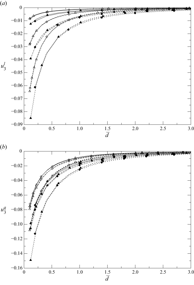
(4.7) \begin{align} \boldsymbol {F}_{\!a}^l&=6\pi \mu a(\ell +\lambda )k_l\big[f_1^l\boldsymbol {e}_1+f_3^l\boldsymbol {e}_3\big],\, \boldsymbol {U}^l=k_l(\ell +\lambda )\big[u_1^l\boldsymbol {e}_1+u_3^l\boldsymbol {e}_3\big], \\[-12pt] \nonumber \end{align}

(4.8) \begin{align} \boldsymbol {F}_{\!a}^q&=6\pi \mu a \ell ^2 k_q\left[f_1^q\boldsymbol {e}_1+f_3^q\boldsymbol {e}_3\right]\!,\, \boldsymbol {U}^q=k_q\big(\ell ^2+a^2/3\big)\left[u_1^q\boldsymbol {e}_1+u_3^q\boldsymbol {e}_3\right]\!, \\[-12pt] \nonumber \end{align}

(4.9) \begin{align} {\boldsymbol\varGamma }_a^l&=4\pi \mu a^3 k_l c_2^l\boldsymbol {e}_2,\, {\boldsymbol \varOmega }^l=k_l\big(w_2^l/2\big)\boldsymbol {e}_2,\, {\boldsymbol\varGamma }_a^q=8\pi \mu a^3\ell k_l c_2^q\boldsymbol {e}_2,\, {\boldsymbol \varOmega }^q=k_q\ell w_2^q\boldsymbol {e}_2. \\[9pt] \nonumber \end{align}

Table 1.

Computed normalised free-space quantities obtained for vanishing ratio $a/\ell$ and given by (4.5), (4.6) and (4.13). The ellipsoid shape parameter is $s=1.2,1.5,2$ and four orientations $\beta$ are considered. Note that $c^{r,0}_{22}$ is independent of $\beta $ .

Each of the above vectors is scaled using the values provided for the sphere immersed in an unbounded fluid by the usual Faxen (Reference Faxen1922, Reference Faxen1923) relations. The ellipsoid behaviour in the addressed shear flows is here characterised by 12 normalised quantities $f_1^l,\ldots ,w_2^q.$ For the triplet $\alpha =(\alpha _0,\alpha _1,\alpha _2)$ let us introduce the Stokes velocity $\boldsymbol {u}^{\alpha }_a=[\alpha _0+\alpha _1 x^{\prime}_3+\alpha _2 (x^{\prime}_3)^2]\boldsymbol {e}_1$ with $x^{\prime}_3=\boldsymbol {x}'\boldsymbol{\cdot }\boldsymbol {e}_3.$ In the absence of a wall (2.14) and (4.3) give the component along ${\tilde {\boldsymbol {e}}}_i$ of the force $\boldsymbol {F}_{\!a}^{nw}$ and of the torque ${\varGamma }_a^{nw}$ exerted on the ellipsoid held fixed in the ambient velocity $\boldsymbol {u}^{\alpha }_a.$ One gets

(4.10) \begin{equation} \boldsymbol {F}_{\!a}^{nw}=16\pi \mu a(\alpha _0 I+\alpha _2 J)\biggl [{{\cos \beta {\tilde {\boldsymbol {e}}}_1}\over {\chi +\alpha _1}} +{{\sin \beta {\tilde {\boldsymbol {e}}}_3}\over {\chi +s^2\alpha _3}}\biggr ],\, {\varGamma }_a^{nw}={{16\pi \mu \alpha _1 a J\boldsymbol {e}_2}\over {\chi -\alpha _2/s^2}} \end{equation}

with, for the ellipsoid selected semi-axis ${\tilde a}_i,$ the following definitions and identities:

(4.11) \begin{equation} I=\int _S {{v{\rm d}S}\over {4\pi a}}=1,\, J=\int _S{{\big[\left(\cos \beta {\tilde x}_3\right)^2+\left(\sin \beta {\tilde x}_1\right)^2\big]v{\rm d}S}\over {4\pi a}}= {{a^2\big(s^2\cos ^2\beta +\sin ^2\beta \big)}\over {3}}. \end{equation}

The force $\boldsymbol {F}_{\!h}^{nw}$ and torque ${\boldsymbol\varGamma }_h^{nw}$ applied on the ellipsoid when it translates at velocity $\boldsymbol {U}={\tilde U}_1{\tilde {\boldsymbol {e}}}_1+{\tilde U}_3{\tilde {\boldsymbol {e}}}_3$ and rotates at velocity ${\boldsymbol \varOmega }=\varOmega _2{\tilde {\boldsymbol {e}}}_2$ in a quiescent and unbounded fluid can be obtained from Oberbeck (Reference Oberbeck1876), Edwardes (Reference Edwardes1892) and Lamb (Reference Lamb1932) and read

(4.12) \begin{equation} \boldsymbol {F}_{\!h}^{nw}=-16\pi \mu a\biggl [{{{\tilde U}_1{\tilde {\boldsymbol {e}}}_1}\over {\chi +\alpha _1}} +{{{\tilde U}_3{\tilde {\boldsymbol {e}}}_3}\over {\chi +s^2\alpha _3}}\biggr ],\, {\boldsymbol\varGamma }_h^{nw}=-{{16\pi \mu a^3(1+s^2)\varOmega _2\boldsymbol {e}_2}\over {3[\chi -\alpha _2/s^2]}}. \end{equation}

Expressing $({\tilde {\boldsymbol {e}}}_1,{\tilde {\boldsymbol {e}}}_3)$ in terms of $\beta$ and $(\boldsymbol {e}_1,\boldsymbol {e}_3),$ using (4.10)–(4.12) and then letting $a/\ell$ vanish provides the quantities $f_1^{l,0},\ldots ,w_2^{q,0}$ associated with those occurring in (4.7)–(4.9) by adequately selecting $\alpha .$ Since not used in this work, the values for the ellipsoid at rest are not reported here. For the freely suspended ellipsoid one arrives at

(4.13) \begin{equation} u_1^{l,0}=u_1^{q,0}=1,\, u_1^{3,0}=u_1^{3,0}=0,\, w_2^{l,0}=w_2^{q,0}={{2 \big(s^2\cos ^2\beta +\sin ^2\beta \big)}\over {1+s^2}}. \end{equation}

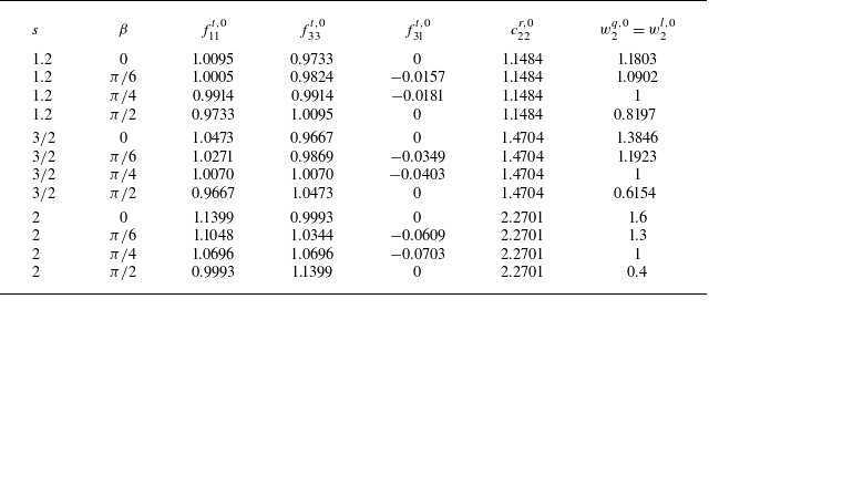
As expected, for the sphere $(s=1)$ each free-space quantity given in (4.5)–(4.6) and (4.13) is either zero or unity. The values of those quantities, calculated with the Maple software, are provided in table 1 for $s=1.2,1.5,2$ and some orientations $\beta $ .

4.2. Numerical implementation and comparisons for a spheroid

In this work the key boundary-integral equation (3.4) is numerically solved by a boundary-element method (BEM). For details regarding this efficient approach the reader is directed to Brebbia, Telles & Wrobel (Reference Brebbia, Telles and Wrobel1984), Pozrikidis (Reference Pozrikidis1992) and Bonnet (Reference Bonnet1995). In contrast to most usual implementations, six-node curved (P2) triangular boundary elements are used to mesh the particle surface. This is done by spreading on this boundary $N$ nodal points at which each Cartesian component of the stress $\boldsymbol {f\!}_a+\boldsymbol {f}$ is unknown. 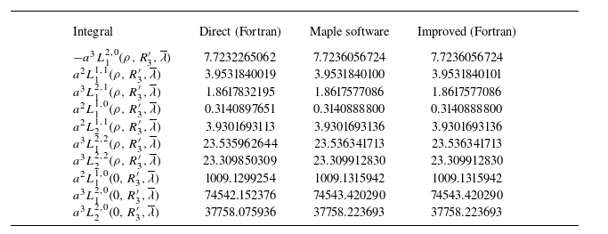The resulting discretised form of (3.4), obtained as explained in detail in Sellier (Reference Sellier2010), is enforced at each node and this yields a $3N$ -equation linear system. Since it has a fully populated and non-symmetric matrix, this linear system is solved with Gaussian elimination. As shown in § 3.2, the Green tensor involves seven Hankel integrals (recall (3.6)–(3.9)) which are accurately computed, with a prescribed accuracy $\epsilon _a,$ by using an iterative Gaussian quadrature briefly explained and tested in Appendix A (see table 6). 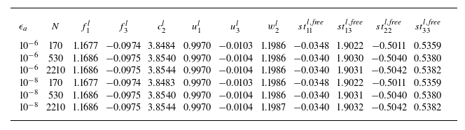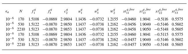For the present work, all the computations have been performed with $\epsilon _a={10^{-6}}$ which is a sufficient accuracy level to provide the normalised friction coefficients and velocity components with a four-digit accuracy (see tables 7 and 8 in Appendix A). When the normalised particle–wall gap ${\overline {d}}=d/a$ becomes small and/or the normalised wall slip length $\overline {\lambda }=\lambda /a$ becomes large a refined mesh is needed. Actually, attention is restricted to the range $\overline {\lambda } \leqslant 5$ because our numerical experiments reveal that the results are nearly unchanged beyond $\overline {\lambda }=5$ . For example, our computations in bipolar coordinates for a sphere translating normal to a plane slip wall (as for table 9 in Appendix C) show that the error $|f^t_{33}(\overline {\lambda }=5)/(f^t_{33}(\overline {\lambda }=\infty )-1|$ is at the most 4 % for $d/a\geqslant 1.0453$ . (The value $f^t_{33}(\overline {\lambda }=\infty )$ is for a plane free surface and has been given in closed form by Brenner (Reference Brenner1961).) This is because, as $\overline {\lambda } \rightarrow \infty$ , the Navier slip condition quickly reduces to the zero-shear condition prevailing on a plane and undisturbed free surface. As later illustrated (see, for instance, tables 7 and 8 in Appendix A), a quite sufficient four-digit accuracy has been obtained for ${\overline {d}}\geqslant O(0.05)$ and $\overline {\lambda }\leqslant O(5)$ using a quite reasonable value of $N.$ More precisely, for the reported results, taking $N\leqslant 3000$ was sufficient and this was made possible by using six-node curved boundary elements.

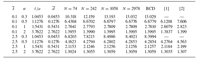
As mentioned in the introduction, accurate numerical results for a sphere with radius $a$ have been obtained using the bipolar coordinates in O’Neill & Bhatt (Reference O’Neill and Bhatt1991), Loussaief et al. (Reference Loussaief, Pasol and Feuillebois2015) and Ghalia et al. (Reference Ghalia, Feuillebois and Sellier2016). Those results permit one to test the accuracy of the present boundary-integral method implementation. A good agreement has been found between the two quite different approaches. Some illustrative results are provided in Appendix C (see tables 9–11). For example, a three-digit accuracy is obtained for the friction coefficient $f_{33}^t$ of a sphere with radius $a$ translating normal to the wall for ${\overline {d}}\sim 0.0453$ and $\overline {\lambda }=2.5$ putting $N=2978$ nodes on the sphere boundary. Finally, the present implementation predictions have been also well compared for a spheroidal body settling near a no-slip wall (Hsu & Ganatos Reference Hsu and Ganatos1994). In that case the Green tensor is the Blake (Reference Blake1971) tensor and the comparisons reported in Sellier (Reference Sellier2005) (see table 1 here) are retrieved.

4.3. Results for a large ellipsoid–wall gap compared with the wall slip length

The normalised quantities introduced in § 4.1 depend on $(s,{\overline {d}},\overline {\lambda },\beta ).$ According to (3.12), for $\epsilon =\lambda /d\ll 1$ each friction coefficient obeys the ‘recipe’ established in § 3.3: it is unchanged, at $O \big(\epsilon ^2 \big),$ when replacing $({\overline {d}},\overline {\lambda })$ with $({\overline {d}}+\overline {\lambda },0).$ When recast in terms of the normalised velocities, (3.13) shows that $(u_1^l, u_3^l)$ and $\omega _2^l$ also obey the ‘recipe’ for the ambient ‘linear’ shear flow. For the ambient quadratic shear flow the ‘recipe’ is not valid. Indeed, (3.14) yields $\text{for }{ k=1,3}$

(4.14) \begin{align} u_k^q({\overline {d}},\overline {\lambda })&=u_k^q({\overline {d}}+\overline {\lambda },0)+{{6\overline {\lambda } \big[u_k^q\left({\overline {d}}+\overline {\lambda },0\right)-u_k^l\left({\overline {d}}+\overline {\lambda },0\right)\big]}\over {3\ell /a+a/\ell }}+O \big(\epsilon ^2 \big); \end{align}

(4.15) \begin{align} \omega _2^q({\overline {d}},\overline {\lambda })&=\omega _2^q({\overline {d}}+\overline {\lambda },0)+\overline {\lambda }\left({{a}\over {\ell }}\right)\big[ \omega _2^q({\overline {d}}+\overline {\lambda },0)-\omega _2^l\left({\overline {d}}+\overline {\lambda },0\right)\big]+O (\epsilon ^2). \end{align}

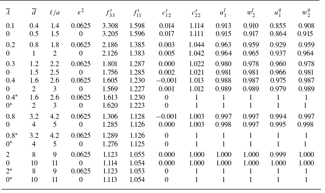
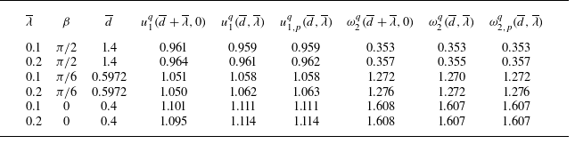
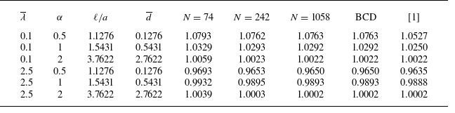
The ‘recipe’ is first numerically tested for a spherical particle and some normalised quantities. Some results are displayed in table 2 for $\lambda /d=0.25$ and ${\overline {d}} \geqslant 0.4$ (i.e. $l/a\geqslant 1.4).$

Table 2.

Some computed normalised quantities for a sphere with radius $a$ and different pairs $(\overline {\lambda },{\overline {d}}).$ Results are given for the wall slip length $\lambda \gt 0$ with wall–sphere gap $d\gg \lambda$ and for the no-slip wall with wall–sphere gap $d+\lambda .$ Here, $\epsilon =\lambda /d=0.25.$ For $l/a\geqslant 2.6$ the asymptotic predictions (4.16) are given in the rows for which the value of $\overline {\lambda }$ has an asterisk.

The reported three-digit values are obtained by the accurate bipolar method. Clearly, the results agree very well for the friction coefficients and $(u_1^l,\omega _2^l)$ with the proposed ‘recipe’ for $\ell /a$ in the considered range $[1.4,11].$ Actually, for $\ell /a$ large and $\overline {\lambda }\leqslant O(1)$ each quantity receives an expansion versus small $a/\ell$ either built from Khabthani et al. (Reference Khabthani, Sellier and Feuillebois2013) or available in Ghalia et al. (Reference Ghalia, Feuillebois and Sellier2016). The estimates derived there for the friction coefficients $f_{11}$ and $f_{33}$ read

(4.16) \begin{equation} f_{kk}=1+f_k\left({{a}\over {\ell }}\right)+f_k[f_k-\overline {\lambda }]\left({{a}\over {\ell }}\right)^2+O\left(\left({{a}\over {\ell }}\right)^3\right),\, f_1={{9}\over {16}},\, f_3={{9}\over {8}}. \end{equation}

Moreover, $c_{12}^t\sim 0$ while the other non-zero quantities are approximated by unity. Note that each approximation (4.16) obeys the ‘recipe’ obtained in § 3.3. The resulting estimates are, for comparison, also provided in table 2 for $\ell /a\geqslant 2.6.$ The results are in full agreement with the predicted ‘recipe’ for the concerned normalised quantities. Remarkably, the velocity $\omega _2^q$ seems to also obey the ‘recipe’ despite (4.15). This is because $\omega _2^q\sim \omega _2^l$ for the sphere (see also the asymptotics provided in Ghalia et al. (Reference Ghalia, Feuillebois and Sellier2016) for $\ell /a$ large). Application of (4.14) supplies values of $u_1^q({\overline {d}},\overline {\lambda })$ close to the reported ones obtained using the bipolar coordinates method. For instance, (4.14) gives $u_1^q(0.4,0.1)=0.8574, u_1^q(0.8,0.2)=0.9311$ and $u_1^q(1.2,0.3)=0.9620.$

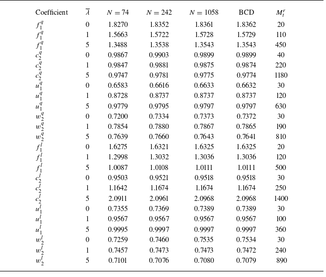
Comparisons have been also made for the considered ellipsoids using the BEM code. For that purpose, a refined mesh on the ellipsoid surface is used so that results with a four-digit accuracy are obtained (see tables 7 and 8).

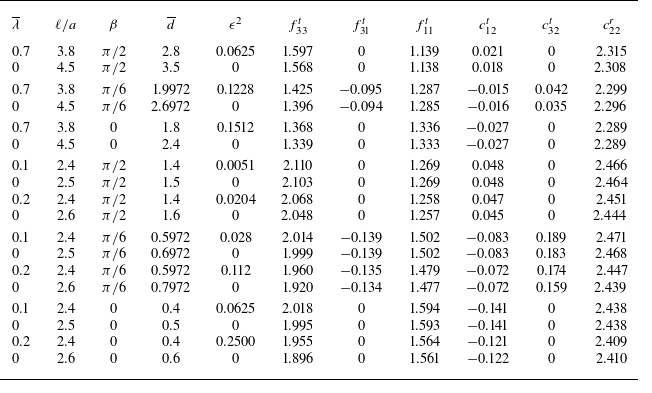
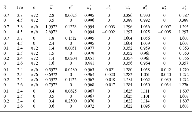
The computed friction coefficients defined by (4.1)–(4.2) are given for the $s=2$ ellipsoid in table 3 for $\lambda /d\leqslant 0.5,$ different orientations $\beta$ and ${\overline {d}} \geqslant 0.4.$ Clearly, each coefficient is seen to nicely obey the proposed ‘recipe’. For the same ellipsoid and settings the normalised velocities defined by (4.7)–(4.9) are provided in table 4.

Table 3.

Computed friction coefficients for the $s=2$ ellipsoid taking a few orientation angles $\beta$ and pairs $(\overline {\lambda },\ell /a).$ The normalised wall–ellipsoid gap ${\overline {d}}=\ell /a-(\sin ^2\beta +s^2\cos ^2\beta )^{1/2}$ (see § 4.1) is indicated and $N=2210$ nodes are put on the ellipsoid boundary. For given $\beta$ the results are reported for a wall slip length $\lambda \gt 0$ with wall–ellipsoid gap $d\gt \lambda$ and for the no-slip wall with wall–ellipsoid gap $d+\lambda .$ Here, $\epsilon =\lambda /d$ .

Table 4.

Counterpart of table 3 giving the normalised velocity components for the $s=2$ ellipsoid freely suspended in a ‘linear’ or quadratic ambient shear flow.

As predicted, the normalised velocities $u_1^l, u_3^l$ and $\omega _2^l$ satisfy the proposed ‘recipe’. The differences $u_1^q({\overline {d}},\overline {\lambda })-u_1^q({\overline {d}}+\overline {\lambda },0)$ are of order $0.01$ and the prediction, $u_{1,p}^q({\overline {d}},\overline {\lambda }),$ from (4.14) is compared, in table 5, with the computed values $u_1^q({\overline {d}},\overline {\lambda })$ and $u_1^q({\overline {d}}+\overline {\lambda },0).$

Table 5.

Computed and predicted (from (4.14)–(4.15)) normalised velocities for the $s=2$ ellipsoid, with location $\ell /a=2.4,$ freely suspended in ambient quadratic shear flow.

It turns out that (4.14) nicely approaches $u_1^q({\overline {d}},\overline {\lambda }).$ Comparisons for the normalised angular velocity predicted by (4.15), $\omega _{2,p}^q({\overline {d}},\overline {\lambda }),$ are also provided in table 5. For $\beta =0$ the predictions are excellent. For $\beta =\pi /6,\pi /2$ the values obtained from (4.15) are pretty good and always below $\omega _{2}^q({\overline {d}}+\overline {\lambda },0)$ as is $\omega _{2}^q({\overline {d}},\overline {\lambda }).$ For these orientations, the small difference $\omega _{2}^q({\overline {d}},\overline {\lambda })-\omega _{2,p}^q({\overline {d}},\overline {\lambda })$ is due to the neglected higher terms in small $\epsilon =\lambda /d.$

4.4. Rigid-body motion of a solid ellipsoid in a quiescent liquid

This subsection considers the rigid-body motion of an ellipsoid in a quiescent liquid. Note that a few results have been given in Feuillebois et al. (Reference Feuillebois, Ghalya and Sellier2012) for the coefficients $f_{11}^t, f_{33}^t, c_{22}^r$ and $c_{12}^t$ only for the $s=1.2$ nearly spherical ellipsoid with orientation $\beta =0$ (see figure 3 b). Those results for $f_{11}^t$ and $f_{33}^t$ are nearly those for the sphere and this is because the $s=1.2$ normalised surface area is $A_{1.2}\sim 1.02$ (recall that all ellipsoids have the sphere volume). A moderate shape sensitivity has been observed (when compared with the sphere) for the coefficients $c_{22}^r$ whatever $l/a$ and for $c_{12}^t$ only near the slip plane. For other orientations and larger values of $s\gt 1$ the coefficients $f_{31}^t$ and $c_{32}^t$ do not necessarily vanish and other trends (shape and orientation effects) are expected for the friction coefficients. This section investigates this key issue, restricting, for conciseness, attention to some $s\gt 1$ ellipsoids.

For given $(s,{\overline {d}}),$ a normalised quantity $\textit {Q}$ (such as the friction coefficients in (4.1)–(4.2), the normalised velocities in (4.7)–(4.9), etc.) can depend on both the particle orientation $\beta$ and the normalised wall slip length $\overline {\lambda }$ in a non-trivial way. This is also the case for the local surface stress $\boldsymbol {f}$ exerted on the particle boundary $S.$ As before, the ${(}0{)}$ superscript is used to designate the value obtained when neglecting the wall–particle interactions. Here, $\delta \boldsymbol {f}=\boldsymbol {f}-\boldsymbol {f}^{{(}0{)}},$ which is due to the interactions with the wall, has a typical magnitude $\delta \!f$ on the part $S_w$ of $S$ where it is not small. Then, the magnitude of $\textit {Q}-\textit {Q}^{(0)}$ is dictated by the product ${\overline S}_w\delta \!f$ , where ${\overline S}_w$ is the area of $S_w.$ For small enough wall–particle gap and slip on the wall, the surface $S_w$ is the part of $S$ located close to the wall. In such circumstances ${\overline S}_w$ increases with $\beta$ (recall figure 3) and $\delta \!f$ increases with $\overline {\lambda }$ so that one can predict the sensitivity of $\textit {Q}-\textit {Q}^{(0)}$ to $(\overline {\lambda },\beta ).$ When $\overline {\lambda }$ is larger the flow on the wall might be even speeded up when compared with the free-space case so that the points of $S_w$ are no longer close to the wall and the behaviour of $\textit {Q}-\textit {Q}^{(0)}$ can become non-trivial.

A numerical analysis has been performed for $s=1.5,2$ and similar new behaviours have been observed. However, $A_{3/2}\sim 1.09$ while $A_{2}\sim 1.26$ so that the shape effects have been found to be more pronounced for $s=2$ than for $s=1.5.$ This is already the case in the absence of a wall, as observed for the free-space coefficients given in table 1 for $s=1.2,1.5,2.$ Indeed, for each coefficient the difference from its value for the sphere $(s=1)$ increases in magnitude as $s$ increases. For conciseness, the results reported in this subsection are for the $s=2$ ellipsoid and, for comparison, for the sphere. The computations for the ellipsoid are achieved using the present BEM approach and stopped at the small value ${\overline {d}}\sim 0.2$ because of numerical limitations, while the bipolar coordinates method (Ghalia et al. Reference Ghalia, Feuillebois and Sellier2016) is used for the sphere and permits one to consider smaller sphere–wall gaps. (Accordingly, in figures 4, 6, 9 and 10 the curves for the sphere are obtained with the bipolar coordinates method and extend to small values of $d.$ )

Figure 4.

Drag coefficients $f^t_{33}$ (a) and $f^t_{11}$ (b) versus the normalised particle–wall gap ${\overline {d}},$ for the $s=2$ ellipsoid translating normal or tangent to a plane slip wall and having orientation $\beta =0$ (square), $\beta =\pi /4$ (triangle) and $\beta =\pi /2$ (circle). The wall has normalised slip length ${\overline \lambda }=0$ (dotted curves), ${\overline \lambda }=0.7$ (dashed curves) and ${\overline \lambda }=5$ (solid curves). For comparison, the results for the sphere (no symbol) are also plotted.

Below the results for all coefficients $f^t_{33}, f^t_{11}, c^r_{22}, c^t_{12}, f^t_{31}$ and $c^t_{32}$ are given versus the normalised particle–wall gap $\overline {d}$ for different orientations $\beta$ and normalised wall slip lengths $\overline {\lambda }.$ Each coefficient depends on $(s,{\overline {d}},\overline {\lambda },\beta ).$ Some coefficients are found to monotonically evolve with increasing $\beta$ in the same fashion whatever ${\overline {d}}.$ Some other coefficients’ sensitivity to $\beta$ depends on ${\overline {d}}.$ For those coefficients additional plots show for ${\overline {d}}=0.2$ the variation of the coefficient versus $\beta$ for different wall slips.

First, the drag coefficients $f_{33}^t$ and $f_{11}^t$ are plotted in figure 4 for the $s=2$ ellipsoid, with orientations $\beta =0,\pi /4,\pi /2,$ and a volume equivalent sphere interacting with a plane with normalised slip $\overline {\lambda }=0,0.7,5.$

The coefficient $f_{33}^t,$ which is a drag coefficient, is positive. The results for $\overline {\lambda }=0.7$ are similar and thus omitted for clarity. As expected, $f_{33}^t$ increases monotonically for decreasing $\overline {d}$ or $\overline {\lambda }.$ In all cases, $f_{33}^t$ strongly depends on the particle location since it slowly tends to its free-space value $f_{33}^{t,0}$ (given in table 1) for large $\overline {d}$ and diverges at contact, as proven by the lubrication analysis for a sphere in Vinogradova (Reference Vinogradova1995) and for an ellipsoid with $\beta =0,\pi /2$ in Vinogradova (Reference Vinogradova1996, Reference Vinogradova1999). Moreover, $f_{33}^t$ is shape-sensitive (compare with the sphere) and shape effects actually depend on the ellipsoid orientation $\beta$ and location ${\overline {d}}$ . For $\beta =\pi /2$ the coefficient $f_{33}^t$ is larger than for the sphere but for $\beta =\pi /4$ it is larger or smaller than for the sphere for $\overline {d}$ large or small, respectively. As far from the wall, $f_{33}^t$ increases with increasing ellipsoid orientation $\beta$ whatever ${\overline {d}}.$ This is because the part of the ellipsoid surface where the friction plays a significant role increases with $\beta$ (see figure 3).

The second drag coefficient $f_{11}^t,$ also plotted in figure 4, is positive and smaller than $f_{33}^t$ as is well known for a sphere near a no-slip wall (O’Neill & Stewartson Reference O’Neill and Stewartson1967; Chaoui & Feuillebois Reference Chaoui and Feuillebois2003). It slowly asymptotes to its free-space value $f_{11}^{t,0}$ (see table 1) as $\overline {d}$ increases. Moreover, starting from $f_{11}^{t,0}$ for the distant wall case it monotonically increases or decreases as $\overline {d}$ drops when the wall slip length is sufficiently small or large (here $\overline {\lambda }=5),$ respectively. For a slip wall $(\overline {\lambda }\gt 0)$ one expects that $f_{11}^t$ has a finite limit at contact, like for the sphere. For instance, it is found in Ghalia et al. (Reference Ghalia, Feuillebois and Sellier2016) that $f_{11}^t\sim 0.98$ at contact for $\overline {\lambda }=5.$ Shape effects are dictated by the orientation $\beta$ (i.e. are weakly dependent on ${\overline {d}}).$ For $\beta =\pi /2$ the coefficient $f_{11}^t$ is slightly (small shape effects) lower than for the sphere whatever the wall slip. In contrast, for $\beta =0$ shape effects occur and $f_{11}^t$ is larger than for the sphere whatever $\overline {d}$ for $\overline {\lambda }=0.7,5$ and either larger or smaller for $\overline {\lambda }=0,$ depending on ${\overline {d}}.$ Not surprisingly, for given $(s,{\overline {d}},\beta )$ the quantity $f_{11}^t$ drops when increasing $\overline {\lambda }.$ Finally, the variation of $f_{11}^t$ with the ellipsoid orientation $\beta$ depends in a non-trivial way on $({\overline {d}},\overline {\lambda }).$ Indeed, for $\overline {d}$ sufficiently large $f_{11}^t$ decreases when increasing $\beta$ whatever the wall slip as is the case in the absence of a wall, but for small enough $\overline {d}$ this behaviour is no longer true.

Figure 5.

Coefficients $f^t_{11}$ and $c^r_{22}$ for the $s=2$ ellipsoid, with orientation $\beta ,$ interacting with a plane slip wall with normalised slip length ${\overline \lambda }=0$ (dotted curves), ${\overline \lambda }=0.7$ (dashed curves) and ${\overline \lambda }=5$ (solid curves). (a) Coefficients $f^t_{11}$ (no symbol) and $c^r_{22}$ (star) versus $\beta /\pi$ for ${\overline {d}}=0.2.$ (b) Coefficient $c^r_{22}$ versus ${\overline {d}}$ for the sphere (no symbol) and the $s=2$ ellipsoid with $\beta =0$ (square), $\beta =\pi /4$ (triangle) and $\beta =\pi /2$ (circle).

This behaviour of $f_{11}^t$ is illustrated for ${\overline {d}}=0.2$ in figure 5 which plots $f_{11}^t$ versus $\beta /\pi$ for $\overline {\lambda }=0,0.7,5.$ For a sufficiently large wall slip $f_{11}^t$ decreases when increasing $\beta$ while for a small slip (here for $\overline {\lambda }=0)$ the coefficient $f_{11}^t$ first slightly decreases and then increases for increasing $\beta .$ This is due to the strong particle–wall interactions, prevailing for a small slip, which apply to a larger part of the ellipsoid surface close to the wall when $\beta$ approaches $\pi /2$ (recall figure 3).

The torque friction coefficient $c_{22}^r$ is also plotted in figure 5 still for $\beta =0,\pi /4,\pi /2$ and $\overline {\lambda }=0,0.7,5.$ It is positive and strongly shape-dependent since for the ellipsoid being about twice that for the sphere, as is the case for the free-space value $c_{22}^{r,0}$ (see table 1). For the sphere, $c_{22}^r$ increases for decaying sphere–wall gap whatever $\overline {\lambda }$ and reaches at contact a finite value only for $\overline {\lambda }\gt 0$ (see O’Neill & Stewartson (Reference O’Neill and Stewartson1967) for the no-slip wall and Loussaief et al. (Reference Loussaief, Pasol and Feuillebois2015) for the slip wall). For the ellipsoid, $c_{22}^r$ varies in a similar way except for a sufficiently large wall slip (here $\overline {\lambda }=5)$ and $\beta =\pi /2.$ In that case, $c_{22}^r$ decreases monotonically as the ellipsoid approaches the wall. Note that $c_{22}^r-c_{22}^{r,0}$ vanishes for large $\overline {d}$ faster for the sphere (for which, see Ghalia et al. (Reference Ghalia, Feuillebois and Sellier2016), it is $O(1/{\overline {d}}^{3})$ ) than for the ellipsoid. As deemed, for both particles $c_{22}^r$ decreases when increasing the wall slip. For $\overline {d}$ small enough and $\overline {\lambda }$ sufficiently small $c_{22}^r$ first increases with $\beta ,$ further decreases with $\beta$ and takes its largest value for $\beta$ close to $\pi /2.$ This property is illustrated in figure 5 for ${\overline {d}}=0.2.$ For other settings $({\overline {d}},\overline {\lambda })$ the coefficient $c_{22}^r$ drops for increasing $\beta$ as is the case in the absence of a wall.

Figure 6.

Friction coefficient $c^t_{12}$ for the $s=2$ ellipsoid, with orientation $\beta ,$ interacting with a plane slip wall with normalised slip length ${\overline \lambda }=0$ (dotted curves), ${\overline \lambda }=0.7$ (dashed curves) and ${\overline \lambda }=5$ (solid curves). (a) Coefficient $c^t_{12}$ versus ${\overline {d}}$ for the sphere (no symbol) and for the $s=2$ ellipsoid with $\beta =0$ (square), $\beta =\pi /4$ (triangle) and $\beta =\pi /2$ . (b) Coefficient $c^t_{12}$ versus $\beta /\pi $ for the $s=2$ ellipsoid and ${\overline {d}}=0.2.$ For comparison, the values for the sphere are indicated as horizontal lines with open circles.

The coupling coefficient $c_{12}^t$ is plotted, still versus $\overline {d}$ and for $\overline {\lambda }=0,0.7,5,$ in figure 6 for three orientations $\beta$ and also versus $\beta /\pi$ for ${\overline {d}}=0.2.$ It is either positive or negative, of rather small magnitude and vanishes slowly as $\overline {d}$ becomes large. As $\overline {d}$ decreases, $|c_{12}^t|$ monotonically increases for the sphere while this is not always the case for the ellipsoid. For example, for a sufficiently small ellipsoid–wall gap it appears that $|c_{12}^t|$ decreases with $d/a$ for $\overline {\lambda }=0.7$ and $\beta =\pi /4.$ At contact the value is finite for each particle. The sensitivity of $c_{12}^t$ to the particle shape is strong: the signs of $c_{12}^t$ for the sphere and for the ellipsoid are different for $\overline {\lambda }=0,5$ while for $\overline {\lambda }=0.7$ and depending on $\overline {d}$ identical signs can be obtained. The variation of $|c_{12}^t|$ with the wall slip is not trivial and strongly depends on the ellipsoid orientation. For instance, if $\beta =0$ then $|c_{12}^t|$ significantly decreases when increasing the slip. In contrast, for $\beta =\pi /2$ then $|c_{12}^t|$ slightly varies and can either increase or decrease with $\overline {\lambda }$ sufficiently small or large, respectively. Moreover, as illustrated in figure 6 for ${\overline {d}}=0.2,$ the quantities $c_{12}^t$ and $|c_{12}^t|$ vary with $\beta$ and $\overline {\lambda }$ in a non-trivial fashion. Clearly, $c_{12}^t$ increases with the orientation $\beta$ whatever the wall slip. For a sufficient slip, $c_{12}^t$ is larger than for the sphere whatever the orientation (here $\overline {\lambda }=5).$ For other slip it is smaller or larger than for the sphere depending on $\beta .$ Let $\beta _c$ be the critical orientation at which $c_{12}^t=0$ for $\overline {\lambda }=0.$ Here, $\beta _c/\pi \sim 0.39$ and for $\beta \gt \beta _c$ then $c_{12}^t$ is positive and increases with $\overline {\lambda }$ which is a somewhat unexpected behaviour because one usually expects a positive friction coefficient to decrease when increasing the slip on the wall. In contrast, for $\beta \lt \beta _c$ there exists a critical normalised slip $\overline {\lambda }_{cr}(\beta )$ for which $c_{12}^t=0$ and then $c_{12}^t$ becomes negative or positive for $\overline {\lambda }\lt \overline {\lambda }_{cr}(\beta )$ or $\overline {\lambda }\gt \overline {\lambda }_{cr}(\beta ),$ respectively. Note that the magnitude of $c_{12}^t$ decreases from its value for the no-slip wall to zero as $\overline {\lambda }$ increases from zero to $\overline {\lambda }_{cr}(\beta )$ and then increases as $\overline {\lambda }$ further increases. In summary, there is a non-trivial sensitivity of $|c_{12}^t|$ to increase of slip on the wall for a given ellipsoid orientation $\beta \lt \beta _c.$

Figure 7.

Coefficients $f^t_{31}$ and $c^t_{32}$ for the $s=2$ ellipsoid, with orientation $\beta ,$ interacting with a plane slip wall with normalised slip length ${\overline \lambda }=0$ (dotted curves), ${\overline \lambda }=0.7$ (dashed curves) and ${\overline \lambda }=5$ (solid curves). (a) Coefficient $f^t_{31}$ versus ${\overline {d}}$ for $\beta =\pi /6$ (diamond) and $\beta =\pi /4$ (triangle). (b) Coefficients $f^t_{31}$ (no symbol) and $c^t_{32}$ (star) versus $\beta /\pi ,$ for ${\overline {d}}=0.2.$

The coefficient $f_{31}^t,$ displayed in figure 7, vanishes for $\beta =0,\pi /2$ and for a sphere. For other ellipsoid orientations it is strictly negative. Therefore, it is strongly shape-dependent. Here, it is plotted for $\beta =\pi /6, \pi /4$ and its magnitude, much smaller than that of the drag force coefficient $f_{33}^t,$ is comparable with that of $c_{12}^t.$ Moreover, $|f_{33}^t|$ vanishes slowly away from the wall and increases as the ellipsoid approaches the slip wall. At contact, $f_{31}^t$ seemingly reaches a finite value. Note that $|f_{31}^t|$ decreases as the slip increases which is a presumable behaviour. Finally, as shown in figure 7, for ${\overline {d}}=0.2,$ the coefficient $f_{31}^t$ first decreases and then further increases when the orientation $\beta$ increases. Therefore, its magnitude admits a largest value for some specific ellipsoid orientation close to $3\pi /10.$ Note that whatever the slip on the wall the plot of $f_{31}^t$ is, notably, nearly (but not exactly) symmetric with respect to the $\theta /\pi =0.25$ vertical line.

Figure 8.

Coefficient $c^t_{32}$ versus $d/a$ for the $s=2$ ellipsoid translating with orientations $\beta =\pi /6$ (diamond) and $\beta =\pi /4$ (triangle) normal to a plane slip wall with normalised slip length ${\overline \lambda }=0$ (dotted curves), ${\overline \lambda }=0.7$ (dashed curves) and ${\overline \lambda }=5$ (solid curves).

Like $f_{31}^t,$ the coupling coefficient $c_{32}^t$ vanishes for a sphere and also, by symmetry, for the ellipsoid with orientation $\beta =0,\pi /2.$ It is plotted in figure 8 for $\beta =\pi /6, \pi /4.$ In contrast to $f_{31}^t,$ it is strictly positive and can be, for small $d/a,$ of significant magnitude. This indicates strong shape effects, near the wall, for this coefficient. Moreover, $c_{32}^t$ slowly vanishes far from the wall and monotonically increases as $\overline {d}$ decreases whatever the wall slip. As for $|f_{31}^t|,$ the coefficient $c_{32}^t$ decreases when increasing the slip. Whatever ${\overline {d}},$ the coefficient $c_{32}^t$ increases and then decreases as the orientation increases. This behaviour is also shown in figure 7 for ${\overline {d}}=0.2.$

4.5. Ellipsoidal particle immersed in a linear or quadratic ambient shear flow

This subsection provides and discusses some results obtained for an ellipsoid freely suspended in a ‘linear’ or quadratic ambient shear flow. For conciseness, the results for the ellipsoid held fixed are not reported. Here, the behaviours of the $s=1.5,2$ ellipsoids are considered and compared with the results obtained for the sphere in Ghalia et al. (Reference Ghalia, Feuillebois and Sellier2016). When freely suspended in the ambient ‘linear’ or quadratic shear flow tangent to the wall, each considered body adopts a translational velocity with normalised components $u_1^l$ (or $u_1^q)$ tangent to the wall and $u_3^l$ (or $u_3^q)$ normal to the wall. Those normalised velocities are introduced in (4.8)–(4.9) and computed with a three-digit accuracy for different settings $(s,{\overline {d}},\overline {\lambda },\beta ).$ For examples and further reference, some results for the $s=1.5$ ellipsoid are displayed in the supplementary material (see the table there) available at https://doi.org/10.1017/jfm.2025.10753.

Figure 9.

Normalised velocity $u_1^q$ versus ${\overline {d}}$ for the freely suspended sphere (no symbols) and the $s=1.5$ (open symbols) and $s=2$ (filled symbols) ellipsoids. Each ellipsoid orientation is $\beta =0\,$ (a, squares), $\beta =\pi /4\,$ (b, triangles) and $\beta =\pi /2\,$ (c, circles). The normalised slip on the plane wall is ${\overline \lambda }=0$ (dotted curves), ${\overline \lambda }=0.7$ (dashed curves) and ${\overline \lambda }=5$ (solid curves).

The normalised velocity $u_1^q$ is plotted in figure 9 for $\beta =0,\pi /4,\pi /2$ and $\overline {\lambda }=0,0.7,5.$ Whatever the ellipsoid, it is positive and quickly tends to unity (recall (4.13)) as $\overline {d}$ increases. For a sphere, $u_1^q\lt 1,$ i.e. the sphere–wall interactions always slow down the sphere. For $s=1.5, 2$ the ellipsoid–wall interactions can speed up the particle ending up with $u_1^q$ slightly above unity. For $s=2$ this is true whatever the slip on the wall for $\beta =0$ with $u_1^q$ increasing as the ellipsoid approaches the wall. This behaviour is modified when increasing the orientation $\beta$ : for instance, for $\beta =\pi /4, \pi /2$ the velocity $u_1^q$ this time decreases with $\overline {d}$ for $\overline {\lambda }=0,0.7.$ The $s=1.5$ ellipsoid behaviour is dictated only by the wall slip: its velocity $u_1^q$ either increases or decreases with decreasing $\overline {d}$ depending on $\overline {\lambda }$ and not on $\beta .$ When it decreases near the wall note that the ellipsoid is slightly slowed down near the wall.

The counterpart of figure 9 for the velocity $u_1^q$ is given in Appendix D (see figure 12). Except for large $\overline {\lambda },$ this time $u_1^q$ always decreases when the particle approaches the wall. Close to a highly slipping wall, $u_1^l$ marginally exceeds unity whatever the shape parameter $s.$

The behaviour of both $u_1^q$ and $u_1^l$ close the wall is considered in figure 10 versus $\beta /\pi$ for the $s=2$ ellipsoid and the small normalised gap ${\overline {d}}=0.2.$ Both velocities clearly depend on the ellipsoid orientation. For small slip $u_1^l$ decreases as $\beta$ increases because the part of the ellipsoid surface subject close to the wall to a large friction increases. For a large slip (here $\overline {\lambda }=5)$ the velocity increases somewhat with the orientation $\beta$ . This is because the wall now exerts a small stress on the part of the ellipsoid surface located in its vicinity. In contrast, $u_1^q$ decreases with increasing $\beta$ whatever the wall slip and for a sufficiently large slip $u_1^q\gt 1$ whatever $\beta .$ For a small or moderate slip (here for $\overline {\lambda }=0,0.7)$ there exists a critical orientation $\beta _c$ at which $u_1^q=1.$ For this ellipsoid orientation there are no global wall–particle interactions and $u_1^q\gt 1$ or $u_1^q\lt 1$ for $\beta \lt \beta _c$ or $\beta \gt \beta _c,$ respectively. Note that for ${\overline {d}}=0.2$ and $\beta /\pi \leqslant 0.22$ the wall–ellipsoid interactions speed up the $s=2$ ellipsoid whatever the slip on the wall, i.e. also for a no-slip wall. This is because for $\beta$ small the part of the ellipsoid surface near point $A$ in figure 3 is subject to a larger ambient velocity. For a large enough slip on the wall (here for $\overline {\lambda }=5)$ the wall–particle interactions speed up the particle $(u_1^q\gt 1)$ whatever its orientation because there is less friction at the point of the ellipsoid surface located close to the wall.

Plots of the angular velocities $\omega _2^q$ and $\omega _2^l$ are available in the supplementary material. It is found that:

1. (i) As $\overline {d}$ increases both velocities are positive and quickly asymptote to $\omega _2^{q,0}$ given by (4.13).

2. (ii) Both velocities are weakly sensitive to the wall slip whatever ${\overline {d}}.$

3. (iii) At a given $\overline {d}$ each velocity strongly depends on the ellipsoid orientation $\beta$ except for $\beta$ close to $\beta =\pi /4.$ For this latter value note that $\partial \omega _2^{l,0}/\partial s=0.$

Plots of the velocities $u_3^l$ and $u_3^q$ are provided and discussed in Appendix D (see figure 13). In the absence of a wall both vanish and the wall–particle interactions are found to increase as $\overline {d}$ decreases and to induce negative velocities of weak magnitude compared with $u_1^l$ and $u_1^q.$

Figure 10.

Normalised velocities $u_1^l $ (triangle) and $u_1^q $ (star) versus $\beta /\pi ,$ for the $s=2$ ellipsoid and ${\overline {d}}=0.2.$ The normalised slip on the plane wall is ${\overline \lambda }=0$ (dotted curves), ${\overline \lambda }=0.7$ (dashed curves) and ${\overline \lambda }=5$ (solid curves).

Figure 11.

Normalised velocities $u_3^l $ (triangle) and $u_3^q $ (star) versus $\beta /\pi $ for the $s=2$ ellipsoid and ${\overline {d}}=0.2$ . The normalised slip on the plane wall is ${\overline \lambda }=0$ (dotted curves), ${\overline \lambda }=0.7$ (dashed curves) and ${\overline \lambda }=5$ (solid curves).

For given $(s,{\overline {d}})$ the sensitivity of $u_3^l$ to $(\overline {\lambda },\beta )$ is the same as that previously found for the coefficient $f^t_{31}$ and illustrated for $s=2$ in figure 7. In the same spirit, figure 11 displays $u_3^l$ and $u_3^q$ versus $\beta /\pi$ for ${\overline {d}}=0.2$ and $\overline {\lambda }=0,0.7,5.$ The comments made for $f^t_{31}$ still hold: $u_3^l$ first decreases and then increases when $\beta$ increases and $|u_3^l|$ decreases, for given $\beta ,$ as $\overline {\lambda }$ increases. Note that whatever the slip on the wall $|u_3^l|$ reaches its maximum for $\beta$ close to $\pi /4.$ Moreover, $u_3^q$ exhibits the same behaviours as $u_3^l.$