1 Introduction
The pressure far field of an object executing small-amplitude motions in a quiescent fluid is a fundamental problem in acoustics, serving as a set-up for examining the production and propagation of sound waves in a fluid. The problem has been studied extensively in the context of continuum mechanics and in various set-ups (Morse Reference Morse1948), characterizing the far-field radiation through the pressure point-wise amplitude and directivity fields. Simplified calculations have been initially presented for an ideal fluid (Morse Reference Morse1948), and extended later on to account for the attenuating impacts of fluid viscosity and heat conductivity (Landau & Lifshitz Reference Landau and Lifshitz1959). In a parallel set of studies, the thermoacoustic sound generation by the unsteady heating of a stationary surface has been examined (see, e.g. McDonald & Wetsel Reference McDonald and Wetsel1978; Yariv & Brenner Reference Yariv and Brenner2004; Hu et al. Reference Hu, Wang, Wu and Wang2012, and works cited therein). This type of acoustic excitation has been applied to develop the thermophone (Arnold & Crandall Reference Arnold and Crandall1917; Wente Reference Wente1922; Shinoda et al. Reference Shinoda, Nakajima, Ueno and Koshida1999) as a means for sound generation with no moving parts.
A key outcome of the above investigations has been the determination of the acoustic waves speed and decay rate. While these have shown to agree well with measurements at low and intermediate frequencies, significant discrepancies have appeared at high frequencies (Greenspan Reference Greenspan1956; Hadjiconstantinou & Garcia Reference Hadjiconstantinou and Garcia2001; Struchtrup Reference Struchtrup2012). These revealed the inadequacy of the continuum description to account for the phase speed and attenuation rate at non-continuum conditions, invoking the study of rarefaction effects on sound wave propagation.
The propagation of sound waves in rarefied gases has been investigated in a considerable number of works. These become relevant wherever the characteristic length scale, or time scale, of the set-up involved is of the order of the molecular mean free path, or time, respectively. In vibroacoustic applications, such scenarios are common in micromechanical oscillators, where short length scales and high frequencies occur (Tamayo Reference Tamayo2005; Bargatin, Kozinsky & Roukes Reference Bargatin, Kozinsky and Roukes2007; Iannacci et al. Reference Iannacci, Huhn, Tschoban and Potter2016). Focusing on a planar vibrating surface (see Sirovich & Thurber Reference Sirovich and Thurber1965; Loyalka & Cheng Reference Loyalka and Cheng1979; Hadjiconstantinou Reference Hadjiconstantinou2002; Manela, Radtke & Pogorelyuk Reference Manela, Radtke and Pogorelyuk2014 and papers cited therein), existing studies have analysed the attenuating effect of gas rarefaction, resulting in decay rates larger than at continuum conditions. Considering a stationary plane, counterpart studies have examined the perturbation field generated by time temperature variations of the boundary (Sone Reference Sone1965; Wadsworth, Erwin & Muntz Reference Wadsworth, Erwin and Muntz1993; Manela & Hadjiconstantinou Reference Manela and Hadjiconstantinou2007, Reference Manela and Hadjiconstantinou2010; Nassios, Yap & Sader Reference Nassios, Yap and Sader2016). Later works have demonstrated that thermoacoustic sound, caused by boundary heat-flux excitations, may be applied for monitoring the sound of a vibrating planar object (Manela & Pogorelyuk Reference Manela and Pogorelyuk2014, Reference Manela and Pogorelyuk2015).
In difference from the above planar set-up investigations, sound wave generation by non-planar objects at rarefied-flow conditions has been studied in only few works. These include the acoustic field analyses of a pulsating cylindrical source carried out by Kalempa & Sharipov (Reference Kalempa and Sharipov2014) and Ben Ami & Manela (Reference Ben Ami and Manela2017), as well as the hydrodynamic perturbations induced by small-amplitude translations of a rigid sphere, considered by Yap & Sader (Reference Yap and Sader2016). Retaining a fixed volume, the sphere translations in Yap & Sader (Reference Yap and Sader2016) were used to model a dipole source, which is of weaker strength than its counterpart volume-varying monopole (Morse Reference Morse1948). It is therefore of interest to complement these studies and consider the vibro- and thermo-acoustic efficiencies of a three-dimensional monopole at non-continuum conditions.
While acknowledging the fundamental interest in studying the canonical pulsating-sphere set-up, the results of such a study may also be of practical value for the analysis of the acoustic field of vibrating nanoscale particles, where both shape and volume variations take form (Pelton et al. Reference Pelton, Sader, Burgin, Liu, Guyot-Sionnest and Gosztola2009; Juvé et al. Reference Juvé, Crut, Maioli, Pellarin, Broyer, Fatti and Vallée2010). In this context, the past decade has evidenced growing interest in the investigation of small-scale micro and nanoparticle vibrations (see Crut et al. (Reference Crut, Maioli, Fatti and Vallée2015), and an abundance of references cited therein). Due to the small size of the particles, quantitative assessment of their internal structural, morphological and mechanical properties requires the application of non-conventional (indirect) measurement techniques. The method of time-resolved spectroscopy is often used for this purpose. The method applies pulsed-laser signals to trigger acoustic oscillations within the particles, through which their properties of interest are captured. The particles response, characterized by their oscillation frequencies and dampening time scales, depends strongly on their interaction with the surrounding medium (Pelton et al. Reference Pelton, Sader, Burgin, Liu, Guyot-Sionnest and Gosztola2009; Marty et al. Reference Marty, Arbouet, Girard, Mlayah, Paillard, Lin, Teo and Tripathy2011). It is therefore of evident importance to study the coupled gas response to acoustic vibrations at small scales, where traditional continuum models break down.
The dynamics of rarefied gas flows is governed by the Boltzmann equation, valid at length and times scales that are larger than the molecular diameter and collision duration, respectively. However, due to the complexity of the kinetic equation, analytical treatments are traditionally limited to the regimes of high (ballistic) and low (continuum-limit) Knudsen (
 $\mathit{Kn}$
) numbers, whereas the intermediate domain of
 $\mathit{Kn}\sim O(1)$
is studied numerically via direct finite-difference-based solutions of the equation or molecular simulations. Notably, the characteristically small excitation amplitudes involved in acoustic problems make the latter approach computationally expensive, and the advantage of obtaining analytical approximations is apparent.
Recent years have shown significant progress in the study of moment equations and their application for the modelling of rarefied gas flows at low and intermediate Knudsen numbers. Originally introduced by Grad (Reference Grad1949), these methods obtain closed-form sets of hydrodynamic-type equations from the Boltzmann equation, in an effort to capture non-small rarefaction effects. Recent progress has been initiated by Struchtrup and Torrilhon (see Struchtrup & Torrilhon (Reference Struchtrup and Torrilhon2003), Struchtrup (Reference Struchtrup2005) and papers cited therein), who formulated the regularized set of thirteen moment equations (R13). Gu & Emerson (Reference Gu and Emerson2007) have complemented the model by deriving the boundary conditions to be imposed at a solid diffuse or specular reflecting surface for Maxwell-type molecules. These conditions have been reassessed by Torrilhon & Struchtrup (Reference Torrilhon and Struchtrup2008), who overcame some inconsistencies prevailing at nonlinear flow conditions. The R13 and higher-order models have been later on applied to investigate a series of steady rarefied gas flows, recently reviewed by Torrilhon (Reference Torrilhon2016). Steady-state solutions for the R13 equations in a spherical geometry were derived by Claydon et al. (Reference Claydon, Shrestha, Rana, Sprittles and Lockerby2017).
In light of the above, the objective of the present contribution is to analyse the effect of gas rarefaction on the acoustic field of a mechanically actuated (through boundary pulsations) and thermally excited (via normal heat-flux) solid sphere. The sphere radius and excitation time scale are chosen so that non-continuum flow conditions prevail, and the problem is investigated in the entire range of gas rarefaction rates. Analytical investigations are carried out in the limits of low (continuum and early transition) and high (free-molecular) Knudsen numbers, and are accompanied by direct simulation Monte Carlo (DSMC) calculations. An analytical solution is derived using the R13 equations, which is found valid at non-small Knudsen numbers (up to
 $\mathit{Kn}\approx 0.6$
) for low enough excitation frequencies. The R13 predictions reveal the appearance of a high-order Knudsen-layer mode, which is missing from the Navier–Stokes description.
In the next section, the pulsating sphere problem is formulated. The analytical treatments in the near-continuum and free-molecular limits are described in §§ 3 and 4, respectively, followed by an outline of the numerical DSMC scheme in § 5. Our results are presented in § 6, where the domains of applicability of the limit-case analyses are delineated, and the acoustic fields of a pulsating adiabatic sphere and a stationary heated surface are described. Concluding remarks are given in § 7.
2 Statement of the problem
Consider a semi-confined monoatomic gas layer of uniform density
 $\unicode[STIX]{x1D70C}_{0}^{\ast }$
and temperature
 $T_{0}^{\ast }$
surrounding an impermeable sphere of radius
 $r^{\ast }=r_{0}^{\ast }$
(hereafter asterisks denote dimensional quantities). The gas is initially at rest and in thermodynamic equilibrium with the sphere. At time
 $t^{\ast }\geqslant 0$
, radial surface pulsations are imposed with velocity
 $$\begin{eqnarray}\unicode[STIX]{x1D700}\boldsymbol{U}_{\boldsymbol{w}}^{\ast }(t^{\ast })=\unicode[STIX]{x1D700}U_{w}^{\ast }(t^{\ast })\hat{\boldsymbol{r}},\end{eqnarray}$$
together with normal heat-flux excitations
 $$\begin{eqnarray}\unicode[STIX]{x1D700}\boldsymbol{Q}_{\boldsymbol{w}}^{\ast }(t^{\ast })=\unicode[STIX]{x1D700}Q_{w}^{\ast }(t^{\ast })\hat{\boldsymbol{r}}.\end{eqnarray}$$
In (2.1) and (2.2),
 $\hat{\boldsymbol{r}}$
marks a unit vector in the radial direction, and
 $\unicode[STIX]{x1D700}\ll 1$
, so that the system description may be linearized about its initial equilibrium. In practice, the monitoring of time-varying heat-flux excitations requires the determination of the amount of energy that is transmitted to the gas. A similar issue, concerning the evaluation of energy transmission efficiency, has been considered in the context of the thermophone device (see Shinoda et al. (Reference Shinoda, Nakajima, Ueno and Koshida1999), Julius et al. (Reference Julius, Gold, Kleiman, Leizeronok and Cukurel2018), and works cited therein). Accordingly, a more comprehensive formulation would couple the thermoacoustic gas state to a heat-conduction problem within the sphere. This calculation would involve the replacement of the boundary condition (2.2) with appropriate matching conditions of heat fluxes and temperatures between the solid and fluid sides of the sphere. The solution of the coupled problem should yield a transfer function relating the amount of invested energy and the heat flux transmitted to the gas, affected by the thermal properties of the solid material. Such an analysis is not followed in the present work, which focuses on the effect of gas rarefaction on monopole sound radiation. In particular, a large portion of our discussion focuses on the generation of sound by an adiabatic (thermally insulating) sphere, which may be easily realized in experiments.
In what follows we analyse the gas response to sphere actuations in the entire range of sphere radii and excitation time scales relative to their counterpart molecular quantities. While the analysis is carried out in part for arbitrary small-amplitude actuations (see § 4), our results are presented for harmonic wall excitations,
 $$\begin{eqnarray}U_{w}^{\ast }(t^{\ast })=\overline{U}_{w}^{\ast }\cos (\unicode[STIX]{x1D714}^{\ast }t^{\ast })\quad \text{and}\quad Q_{w}^{\ast }(t^{\ast })=\overline{Q}_{w}^{\ast }\cos (\unicode[STIX]{x1D714}^{\ast }t^{\ast }),\end{eqnarray}$$
where
 $\unicode[STIX]{x1D714}^{\ast }$
denotes the common mechanical and heat-flux actuation frequency, and we focus on the final time-periodic state of the system. Here,
 $\unicode[STIX]{x1D700}$
has been omitted for convenience, yet the numerical values of
 $\overline{U}_{w}^{\ast }$
and
 $\overline{Q}_{w}^{\ast }$
will be taken small in their normalized form.
Further analysis requires the scaling of the problem. To this end we normalize the length and velocity by the nominal sphere radius
 $r_{0}^{\ast }$
and molecular mean thermal speed
 $U_{th}^{\ast }=\sqrt{2{\mathcal{R}}^{\ast }T_{0}^{\ast }}$
(where
 ${\mathcal{R}}^{\ast }$
marks the specific gas constant), respectively. The non-dimensional problem is then governed by the gas mean Knudsen number and scaled frequency,
 $$\begin{eqnarray}\mathit{Kn}=l_{0}^{\ast }/r_{0}^{\ast }\quad \text{and}\quad \unicode[STIX]{x1D714}=\unicode[STIX]{x1D714}^{\ast }r_{0}^{\ast }/U_{th}^{\ast },\end{eqnarray}$$
respectively, where
 $l_{0}^{\ast }$
marks the molecular mean free path, specified after (3.8). In terms of the governing parameters, it is expected that free-molecular conditions should prevail when
 $\mathit{Kn}\gg 1$
or
 $\unicode[STIX]{x1D714}\mathit{Kn}\gg 1$
, for which either the length scale or time scale is short compared with the mean free path or mean free time, respectively. In contrast, as will be discussed in § 6, continuum-limit conditions require that both
 $\mathit{Kn}\ll 1$
and
 $\unicode[STIX]{x1D714}^{2}\mathit{Kn}\ll 1$
. For later convenience we denote
 $$\begin{eqnarray}\mathit{Kn}_{\unicode[STIX]{x1D714}}=\unicode[STIX]{x1D714}\mathit{Kn}=\unicode[STIX]{x1D714}^{\ast }l_{0}^{\ast }/U_{th}^{\ast },\end{eqnarray}$$
as the frequency-based Knudsen number, representing the ratio between the excitation frequency and the molecular collision frequency. The following analysis will be presented in terms of
 $\mathit{Kn}$
and
 $\unicode[STIX]{x1D714}$
, while
 $\mathit{Kn}_{\unicode[STIX]{x1D714}}$
will be used to facilitate the discussion in § 6.
To better assess the effect of gas rarefaction on the acoustic efficiency of the source, we recapitulate the known result for the acoustic field of a pulsating sphere at continuum inviscid (
 $\mathit{Kn},\unicode[STIX]{x1D714}\mathit{Kn}\rightarrow 0$
) conditions (Morse Reference Morse1948). Considering the case of harmonic mechanical actuations only (
 $\overline{U}_{w}\neq 0,\overline{Q}_{w}=0$
), the far-field acoustic pressure and radial velocity are given by
 $$\begin{eqnarray}\left.\begin{array}{@{}c@{}}\displaystyle p_{inviscid}(r,t)=\frac{\overline{U}_{w}\unicode[STIX]{x1D714}}{r(1+\unicode[STIX]{x1D714}^{2}/c_{0}^{2})}\left[\frac{\unicode[STIX]{x1D714}}{c_{0}}\cos (\unicode[STIX]{x1D714}t_{r})-\sin (\unicode[STIX]{x1D714}t_{r})\right]\quad \text{and}\\ \displaystyle u_{inviscid}(r,t)=\frac{\overline{U}_{w}\unicode[STIX]{x1D714}}{rc_{0}(1+\unicode[STIX]{x1D714}^{2}/c_{0}^{2})}\left[\frac{\unicode[STIX]{x1D714}}{c_{0}}\left(\frac{c_{0}^{2}}{\unicode[STIX]{x1D714}^{2}r}+1\right)\cos (\unicode[STIX]{x1D714}t_{r})+\left(\frac{1}{r}-1\right)\sin (\unicode[STIX]{x1D714}t_{r})\right]\!,\end{array}\right\}\end{eqnarray}$$
respectively, where
 $t_{r}=t-(r-1)/c_{0}$
is the acoustic retarded time (with
 $r$
denoting the scaled radial distance from the sphere centre), and
 $c_{0}$
marks the mean speed of sound scaled by the mean thermal speed,
 $c_{0}^{\ast }/U_{th}^{\ast }$
. For an ideal monatomic gas considered hereafter,
 $c_{0}^{\ast }=\sqrt{\unicode[STIX]{x1D6FE}{\mathcal{R}}^{\ast }T_{0}^{\ast }}$
(where
 $\unicode[STIX]{x1D6FE}=5/3$
marks the ratio of gas specific heats), and
 $c_{0}=\sqrt{5/6}$
. The overall source strength is evaluated through its acoustic power
 $$\begin{eqnarray}\unicode[STIX]{x1D6F1}(r,t)\equiv \oint _{\tilde{r}=r}p(\tilde{r},t)u(\tilde{r},t)\,\text{d}S,\end{eqnarray}$$
where the integration is carried out over a spherical surface
 $S$
of radius
 $\tilde{r}>1$
centred at
 $\tilde{r}=0$
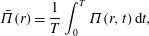
. To obtain a time-independent result, we define the time-averaged acoustic power,
 $$\begin{eqnarray}\bar{\unicode[STIX]{x1D6F1}}(r)=\frac{1}{T}\int _{0}^{T}\unicode[STIX]{x1D6F1}(r,t)\,\text{d}t,\end{eqnarray}$$
obtained by integrating
 $\unicode[STIX]{x1D6F1}(r,t)$
over a period
 $T=2\unicode[STIX]{x03C0}/\unicode[STIX]{x1D714}$
. Substituting (2.6) into (2.7) and then into (2.8), we obtain for the inviscid far-field limit
 $$\begin{eqnarray}\bar{\unicode[STIX]{x1D6F1}}_{inviscid}(r\gg 1)\approx 2\unicode[STIX]{x03C0}\overline{U}_{w}^{2}\sqrt{\frac{6}{5}}\left(\frac{\unicode[STIX]{x1D714}^{2}}{1+6\unicode[STIX]{x1D714}^{2}/5}\right).\end{eqnarray}$$
The result is independent of
 $r\gg 1$
due to the
 $r^{-1}$
leading-order decay of
 $p_{inviscid}$
and
 $u_{inviscid}$
, and thus remains unchanged at arbitrarily large distances from the source. As will be shown in §§ 3 and 4, non-zero gas rarefaction results in stronger decay rates which, in turn, lead to a decrease in (and far-field vanishing of) the acoustic power with increasing
 $r$
(see figure 7).
3 Near-continuum conditions
To analyse the problem at relatively small Knudsen numbers, we make use of the hydrodynamic R13 model mentioned in § 1 (Struchtrup & Torrilhon Reference Struchtrup and Torrilhon2003; Struchtrup Reference Struchtrup2005). The scheme has been derived for a Maxwell-type model of molecular interaction, where the three-dimensional formulation consists of balances for the scalar density and pressure, the vectors of velocity and heat flux and the stress tensor. Higher-order moments are coupled to the system through a Chapman–Enskog-type expansion of the probability density function in the kinetic Boltzmann equation. In this work, we apply the R13 model for an unsteady, one-dimensional (
 $r$
-dependent) and linearized set-up. Focusing on the case of sinusoidal excitation specified in (2.3), we assume harmonic time dependence of all hydrodynamic perturbations,
 $$\begin{eqnarray}\unicode[STIX]{x1D6F7}(r,t)=Re\{\overline{\unicode[STIX]{x1D6F7}}(r)\exp [\text{i}\unicode[STIX]{x1D714}t]\}.\end{eqnarray}$$
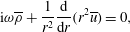
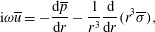
Using spherical coordinates, the macroscopic balances of continuity,
 $r$
-momentum and energy are given by
 $$\begin{eqnarray}\displaystyle & \displaystyle \text{i}\unicode[STIX]{x1D714}\overline{\unicode[STIX]{x1D70C}}+\frac{1}{r^{2}}\frac{\text{d}}{\text{d}r}(r^{2}\overline{u})=0, & \displaystyle\end{eqnarray}$$
 $$\begin{eqnarray}\displaystyle & \displaystyle \text{i}\unicode[STIX]{x1D714}\overline{u}=-\frac{\text{d}\overline{p}}{\text{d}r}-\frac{1}{r^{3}}\frac{\text{d}}{\text{d}r}(r^{3}\overline{\unicode[STIX]{x1D70E}}), & \displaystyle\end{eqnarray}$$
and
 $$\begin{eqnarray}\text{i}\unicode[STIX]{x1D714}\overline{T}=-\frac{2}{3r^{2}}\frac{\text{d}}{\text{d}r}[r^{2}(\overline{u}+2\overline{q})],\end{eqnarray}$$
respectively, and are supplemented by the linearized form of the equation of state,
 $$\begin{eqnarray}\overline{p}=(\overline{\unicode[STIX]{x1D70C}}+\overline{T})/2.\end{eqnarray}$$
Appearing in (3.2)–(3.5) are the amplitudes of the density perturbation
 $\overline{\unicode[STIX]{x1D70C}}(r)$
, radial velocity
 $\overline{u}(r)$
, pressure
 $\overline{p}(r)$
and temperature
 $\overline{T}(r)$
. Also appearing in (3.3)–(3.4) are the amplitudes of the radial normal stress
 $\overline{\unicode[STIX]{x1D70E}}(r)$
, and the radial heat flux
 $\overline{q}(r)$
, which satisfy the additional equations
 $$\begin{eqnarray}\text{i}\unicode[STIX]{x1D714}\overline{\unicode[STIX]{x1D70E}}+\frac{1}{r^{4}}\frac{\text{d}}{\text{d}r}(r^{4}\overline{m})=-\frac{\overline{\unicode[STIX]{x1D70E}}}{2\mathit{Kn}}-\frac{2r}{3}\frac{\text{d}}{\text{d}r}\left[r^{-1}\left(\overline{u}+\frac{4}{5}\overline{q}\right)\right]\end{eqnarray}$$
and
 $$\begin{eqnarray}\text{i}\unicode[STIX]{x1D714}\overline{q}+\frac{1}{2r^{3}}\frac{\text{d}}{\text{d}r}(r^{3}\overline{R})=-\frac{\overline{q}}{3\mathit{Kn}}-\frac{1}{2r^{3}}\frac{\text{d}}{\text{d}r}(r^{3}\overline{\unicode[STIX]{x1D70E}})-\frac{5}{8}\frac{\text{d}\overline{T}}{\text{d}r}-\frac{1}{6}\frac{\text{d}\overline{\unicode[STIX]{x1D6E5}}}{\text{d}r}.\end{eqnarray}$$
Equations (3.6) and (3.7) couple the higher-order moments’ amplitude functions
 $\overline{m}(r)$
,
 $\overline{R}(r)$
and
 $\overline{\unicode[STIX]{x1D6E5}}(r)$
, which are fixed through a linearized form of the closure relations derived by Struchtrup & Torrilhon (Reference Struchtrup and Torrilhon2003),
 $$\begin{eqnarray}\overline{m}=-\frac{6\mathit{Kn}}{5}r^{2}\frac{\text{d}}{\text{d}r}(r^{-2}\overline{\unicode[STIX]{x1D70E}}),\quad \overline{R}=-\frac{16\mathit{Kn}}{5}r\frac{\text{d}}{\text{d}r}(r^{-1}\overline{q})\quad \text{and}\quad \overline{\unicode[STIX]{x1D6E5}}=-\frac{12\mathit{Kn}}{r^{2}}\frac{\text{d}}{\text{d}r}(r^{2}\overline{q}).\end{eqnarray}$$
The Knudsen number appearing in (3.6)–(3.8) is given by
 $$\begin{eqnarray}\mathit{Kn}=\unicode[STIX]{x1D708}_{0}^{\ast }/r_{0}^{\ast }U_{th}^{\ast },\end{eqnarray}$$
where
 $l_{0}^{\ast }=\unicode[STIX]{x1D708}_{0}^{\ast }/U_{th}^{\ast }$
in accordance with (2.4). At continuum-limit conditions,
 $\unicode[STIX]{x1D708}_{0}^{\ast }$
marks the coefficient of kinematic viscosity. Equations (3.2)–(3.8) are supplemented by the conditions of impermeability and normal heat flux at the sphere surface (see (2.1)–(2.2)),
 $$\begin{eqnarray}\overline{u}(1)=\overline{U}_{w}\quad \text{and}\quad \overline{q}(1)=\overline{Q}_{w},\end{eqnarray}$$
together with a high-order moment condition obtained from Gu & Emerson (Reference Gu and Emerson2007),
 $$\begin{eqnarray}-\frac{6}{\sqrt{\unicode[STIX]{x03C0}}}\overline{\unicode[STIX]{x1D70E}}(1)-\frac{6}{7\sqrt{\unicode[STIX]{x03C0}}}\overline{R}(1)-4\overline{m}(1)=\overline{U}_{w}+\frac{4}{5}\overline{Q}_{w},\end{eqnarray}$$
and far-field decay conditions. As expected, a temperature jump condition is missing from the present formulation, and is replaced by the heat-flux condition in (3.10). The condition (3.11) is derived by eliminating the unknown wall temperature from the linearized version of conditions (30) and (31) in Gu & Emerson (Reference Gu and Emerson2007) (or, alternatively, equations (35) and (36) in Torrilhon & Struchtrup (Reference Torrilhon and Struchtrup2008)). Note that in both Gu & Emerson (Reference Gu and Emerson2007) and Torrilhon & Struchtrup (Reference Torrilhon and Struchtrup2008), the boundary considered is not shifted in the normal direction, different from the present set-up. Hence, the wall normal velocity contribution should be added, similarly to Rana, Lockerby & Sprittles (Reference Rana, Lockerby and Sprittles2018) and Beckmann et al. (Reference Beckmann, Rana, Torrilhon and Struchtrup2018), in the context of evaporation-driven flows.
The system of equations may be recast to form a single triharmonic equation for
 $\overline{T}(r)$
,
 $$\begin{eqnarray}\displaystyle & & \displaystyle \mathit{Kn}^{3}\left[1+{\textstyle \frac{36}{5}}\text{i}\unicode[STIX]{x1D714}\mathit{Kn}\right]\unicode[STIX]{x1D6FB}_{r}^{6}\overline{T}-{\textstyle \frac{5}{12}}\mathit{Kn}\left[1+{\textstyle \frac{62}{5}}\text{i}\unicode[STIX]{x1D714}\mathit{Kn}-{\textstyle \frac{888}{25}}(\unicode[STIX]{x1D714}\mathit{Kn})^{2}-{\textstyle \frac{2592}{125}}\text{i}(\unicode[STIX]{x1D714}\mathit{Kn})^{3}\right]\unicode[STIX]{x1D6FB}_{r}^{4}\overline{T}\nonumber\\ \displaystyle & & \displaystyle \qquad +\,{\textstyle \frac{5}{18}}\text{i}\unicode[STIX]{x1D714}\left[1+{\textstyle \frac{48}{5}}\text{i}\unicode[STIX]{x1D714}\mathit{Kn}-{\textstyle \frac{864}{25}}(\unicode[STIX]{x1D714}\mathit{Kn})^{2}-{\textstyle \frac{864}{25}}\text{i}(\unicode[STIX]{x1D714}\mathit{Kn})^{3}\right]\unicode[STIX]{x1D6FB}_{r}^{2}\overline{T}\nonumber\\ \displaystyle & & \displaystyle \qquad +\,{\textstyle \frac{1}{3}}\text{i}\unicode[STIX]{x1D714}^{3}[1+5\text{i}\unicode[STIX]{x1D714}\mathit{Kn}-6(\unicode[STIX]{x1D714}\mathit{Kn})^{2}]\overline{T}=0,\end{eqnarray}$$
where
 $\unicode[STIX]{x1D6FB}_{r}^{2}=r^{-2}(\text{d}/\text{d}r)(r^{2}(\text{d}/\text{d}r))$
denotes the
 $r$
-dependent part of the Laplace operator. The equation is subject to the solution
 $$\begin{eqnarray}\overline{T}(r)=\mathop{\sum }_{n=1}^{6}\unicode[STIX]{x1D6FC}_{n}\unicode[STIX]{x1D6E9}_{n}(r),\end{eqnarray}$$
where
 $\unicode[STIX]{x1D6FC}_{n}$
are constants and
 $\unicode[STIX]{x1D6E9}_{n}(r)$
satisfy the Helmholtz equation
 $$\begin{eqnarray}\unicode[STIX]{x1D6FB}_{r}^{2}\unicode[STIX]{x1D6E9}_{n}=\unicode[STIX]{x1D706}_{n}^{2}\unicode[STIX]{x1D6E9}_{n}.\end{eqnarray}$$
In (3.14),
 $\unicode[STIX]{x1D706}_{n}$
are the roots of the characteristic polynomial of (3.12). Expanding in
 $\mathit{Kn}\ll 1$
, the leading-order expressions for
 $\unicode[STIX]{x1D706}_{n}$
are
 $$\begin{eqnarray}\left.\begin{array}{@{}c@{}}\displaystyle \unicode[STIX]{x1D706}_{1\pm }\approx \pm \sqrt{\frac{6}{5}}\left(\frac{7}{5}\unicode[STIX]{x1D714}^{2}\mathit{Kn}+\text{i}\unicode[STIX]{x1D714}\right),\quad \unicode[STIX]{x1D706}_{2\pm }\approx \pm \sqrt{\frac{1}{3}\frac{\unicode[STIX]{x1D714}}{\mathit{Kn}}}(1+\text{i})\quad \text{and}\\ \displaystyle \unicode[STIX]{x1D706}_{3\pm }\approx \pm \sqrt{15}\left(\frac{1}{6}\mathit{Kn}^{-1}+\frac{3}{10}\text{i}\unicode[STIX]{x1D714}\right),\end{array}\right\}\end{eqnarray}$$
and the general solution for
 $\overline{T}(r)$
may be put in the form
 $$\begin{eqnarray}\overline{T}(r)=\mathop{\sum }_{n=1}^{3}\left\{a_{n}\frac{\sin (\text{i}\unicode[STIX]{x1D706}_{n}r)}{\text{i}\unicode[STIX]{x1D706}_{n}r}+b_{n}\frac{\cos (\text{i}\unicode[STIX]{x1D706}_{n}r)}{\text{i}\unicode[STIX]{x1D706}_{n}r}\right\}.\end{eqnarray}$$
Expecting a casual outward radiating signal, we set
 $a_{n}=\text{i}b_{n}$
, which ensures that no incoming propagating wave is contained, to yield
 $$\begin{eqnarray}\overline{T}(r)=\mathop{\sum }_{n=1}^{3}C_{n}\frac{\exp [-\unicode[STIX]{x1D706}_{n}r]}{r}.\end{eqnarray}$$
For later reference, we denote the
 $\unicode[STIX]{x1D706}_{1},\unicode[STIX]{x1D706}_{2}$
and
 $\unicode[STIX]{x1D706}_{3}$
components of the solution the ‘compression’, ‘thermal’ and ‘Knudsen-layer’ modes, respectively. The compression mode is characterized by the slowest decay rate at low
 $\mathit{Kn}$
, and therefore dominates the far-field response, whereas the thermal and Knudsen-layer components decay much stronger. In particular, the Knudsen-layer mode decays at rate
 ${\sim}\exp [-\sqrt{15}\mathit{Kn}^{-1}r/6]$
, and is therefore significant only in an
 $O(\mathit{Kn})$
(Knudsen-layer) vicinity of the wall. Yet, apart from its direct effect on the gas behaviour inside the layer, it affects the values of the constants
 $C_{1}$
and
 $C_{2}$
multiplying the
 $\unicode[STIX]{x1D706}_{1,2}$
modes, which then modify the gas behaviour in the entire domain. For later discussion we note that the leading-order decay rate of
 $\unicode[STIX]{x1D706}_{3}$
is independent of the excitation frequency, and is therefore not affected by a change in the system time scale.
Having solved for
 $\overline{T}(r)$
, expressions for all other hydrodynamic fields follow by substitutions of (3.17) into the above set of balance equations, as specified in appendix A. Importantly, all fields combine the three decaying components contained in (3.17). The constants
 $C_{n}$
are fixed using the conditions in (3.10) and (3.11).
3.1 The Navier–Stokes–Fourier limit
To assess the differences between the R13 and continuum-limit solutions, it is instructive to derive the Navier–Stokes–Fourier (NSF) description of the system. Either by replacing (3.6) and (3.7) with the Newtonian and Fourier constitutive relations for
 $\overline{\unicode[STIX]{x1D70E}}(r)$
and
 $\overline{q}(r)$
, respectively, or by taking the consistent
 $Kn\ll 1$
leading-order limit of (3.12), the problem for
 $\overline{T}(r)$
reduces to the biharmonic equation
 $$\begin{eqnarray}\frac{5}{4}\mathit{Kn}\unicode[STIX]{x1D6FB}_{r}^{4}\overline{T}+\frac{\unicode[STIX]{x1D714}}{6}(-5\text{i}+23\unicode[STIX]{x1D714}\mathit{Kn})\unicode[STIX]{x1D6FB}_{r}^{2}\overline{T}-\text{i}\unicode[STIX]{x1D714}^{3}\overline{T}=0.\end{eqnarray}$$
Different from the R13 result, the reduction in the equation order leads to the solution
 $$\begin{eqnarray}\overline{T}(r)=\mathop{\sum }_{n=1}^{2}D_{n}\frac{\exp [-\unicode[STIX]{x1D706}_{n}^{NSF}r]}{r},\end{eqnarray}$$
where
 $$\begin{eqnarray}\unicode[STIX]{x1D706}_{1\pm }^{NSF}\approx \pm \sqrt{\frac{6}{5}}\left(\frac{7}{5}\unicode[STIX]{x1D714}^{2}\mathit{Kn}+\text{i}\unicode[STIX]{x1D714}\right)\quad \text{and}\quad \unicode[STIX]{x1D706}_{2\pm }^{NSF}\approx \pm \sqrt{\frac{1}{3}\frac{\unicode[STIX]{x1D714}}{\mathit{Kn}}}(1+\text{i})\end{eqnarray}$$
are the roots of the characteristic polynomial corresponding to (3.18).
Inspecting the similarities between the NSF and R13 results, we observe that the leading orders of
 $\unicode[STIX]{x1D706}_{1,2}$
in (3.15) and
 $\unicode[STIX]{x1D706}_{1,2}^{NSF}$
in (3.20) are identical. The higher-order corrections, not specified here for brevity, differ in some quantitative details. Yet more importantly, the reduction in problem order in the NSF model results in the omission of the
 $\unicode[STIX]{x1D706}_{3}$
mode from the NSF description. At small enough
 $\mathit{Kn}$
, these differences have only a minor effect on the results, as the Knudsen layer (and its associated outer-layer impact) diminishes. At non-vanishing
 $\mathit{Kn}$
, however, the effect of the Knudsen layer becomes significant, contributing to the breakdown of the NSF description. As demonstrated by the results in § 6, the R13 model remains valid in part of these parameter combinations, yielding predictions that are in agreement with DSMC computations.
4 Free-molecular limit
Free-molecular conditions should prevail wherever
 $\mathit{Kn}\gg 1$
or
 $\mathit{Kn}_{\unicode[STIX]{x1D714}}=\unicode[STIX]{x1D714}\mathit{Kn}\gg 1$
, for which either the length scale or time scale is short compared with the mean free path or mean free time, respectively. For the spherically symmetric set-up considered, the gas state is governed by the probability density function
 $f=f(r,t,\unicode[STIX]{x1D743})$
of finding a gas molecule with velocity and radial position about
 $\unicode[STIX]{x1D743}$
and
 $r$
, respectively, at time
 $t$
. Expanding
 $f(r,t,\unicode[STIX]{x1D743})$
about its initial non-dimensional Maxwellian distribution
 $F=\unicode[STIX]{x03C0}^{-3/2}\exp [-\unicode[STIX]{x1D709}^{2}]$
, we write
 $$\begin{eqnarray}f(r,t,\unicode[STIX]{x1D743})=F[1+h(r,t,\unicode[STIX]{x1D743})],\end{eqnarray}$$
where
 $h(r,t,\unicode[STIX]{x1D743})$
denotes the unknown small (
 $|h|\ll 1$
) perturbation function due to sphere excitations. At free-molecular conditions,
 $h(r,t,\unicode[STIX]{x1D743})$
satisfies the collisionless one-dimensional (
 $r$
-dependent) Boltzmann equation in spherical coordinates
 $(r,\unicode[STIX]{x1D703},\unicode[STIX]{x1D711})$
(Kogan Reference Kogan1969),
 $$\begin{eqnarray}\frac{\unicode[STIX]{x2202}h}{\unicode[STIX]{x2202}t}+\unicode[STIX]{x1D709}_{r}\frac{\unicode[STIX]{x2202}h}{\unicode[STIX]{x2202}r}+\frac{\unicode[STIX]{x1D709}_{\unicode[STIX]{x1D703}}^{2}+\unicode[STIX]{x1D709}_{\unicode[STIX]{x1D711}}^{2}}{r}\frac{\unicode[STIX]{x2202}h}{\unicode[STIX]{x2202}\unicode[STIX]{x1D709}_{r}}+\frac{1}{r}\left(\frac{\unicode[STIX]{x1D709}_{\unicode[STIX]{x1D711}}^{2}}{\tan \unicode[STIX]{x1D703}}-\unicode[STIX]{x1D709}_{r}\unicode[STIX]{x1D709}_{\unicode[STIX]{x1D703}}\right)\frac{\unicode[STIX]{x2202}h}{\unicode[STIX]{x2202}\unicode[STIX]{x1D709}_{\unicode[STIX]{x1D711}}}-\frac{\unicode[STIX]{x1D709}_{\unicode[STIX]{x1D711}}}{r}\left(\frac{\unicode[STIX]{x1D709}_{\unicode[STIX]{x1D703}}}{\tan \unicode[STIX]{x1D703}}+\unicode[STIX]{x1D709}_{r}\right)\frac{\unicode[STIX]{x2202}h}{\unicode[STIX]{x2202}\unicode[STIX]{x1D709}_{\unicode[STIX]{x1D711}}}=0,\end{eqnarray}$$
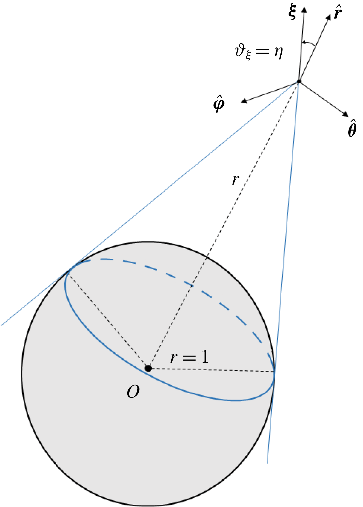
where the system parametrization is specified in figure 1. Performing the variable transformation
 $$\begin{eqnarray}\unicode[STIX]{x1D709}=\sqrt{\unicode[STIX]{x1D709}_{r}^{2}+\unicode[STIX]{x1D709}_{\unicode[STIX]{x1D703}}^{2}+\unicode[STIX]{x1D709}_{\unicode[STIX]{x1D711}}^{2}},\quad \cos \unicode[STIX]{x1D717}_{\unicode[STIX]{x1D709}}=\frac{\unicode[STIX]{x1D709}_{r}}{\unicode[STIX]{x1D709}}\quad \text{and}\quad \tan \unicode[STIX]{x1D719}_{\unicode[STIX]{x1D709}}=\frac{\unicode[STIX]{x1D709}_{\unicode[STIX]{x1D703}}}{\unicode[STIX]{x1D709}_{\unicode[STIX]{x1D711}}},\end{eqnarray}$$
equation (4.2) assumes the form
 $$\begin{eqnarray}\frac{\unicode[STIX]{x2202}h}{\unicode[STIX]{x2202}t}+\unicode[STIX]{x1D709}\cos \unicode[STIX]{x1D717}_{\unicode[STIX]{x1D709}}\frac{\unicode[STIX]{x2202}h}{\unicode[STIX]{x2202}r}-\frac{\unicode[STIX]{x1D709}\sin \unicode[STIX]{x1D717}_{\unicode[STIX]{x1D709}}}{r}\frac{\unicode[STIX]{x2202}h}{\unicode[STIX]{x2202}\unicode[STIX]{x1D717}_{\unicode[STIX]{x1D709}}}+\tan \unicode[STIX]{x1D703}\frac{\unicode[STIX]{x1D709}\sin \unicode[STIX]{x1D717}_{\unicode[STIX]{x1D709}}\cos \unicode[STIX]{x1D719}_{\unicode[STIX]{x1D709}}}{r}\frac{\unicode[STIX]{x2202}h}{\unicode[STIX]{x2202}\unicode[STIX]{x1D719}_{\unicode[STIX]{x1D709}}}=0.\end{eqnarray}$$
The equation is supplemented by the initial condition
 $$\begin{eqnarray}h(r,t=0^{-},\unicode[STIX]{x1D709},\unicode[STIX]{x1D717}_{\unicode[STIX]{x1D709}},\unicode[STIX]{x1D719}_{\unicode[STIX]{x1D709}})=0,\end{eqnarray}$$
together with a linearized form of the diffuse boundary condition at the spherical surface,
 $$\begin{eqnarray}h(r=1,0\leqslant \unicode[STIX]{x1D717}_{\unicode[STIX]{x1D709}}\leqslant \unicode[STIX]{x03C0}/2)=\unicode[STIX]{x1D70C}_{w}(t)+2\unicode[STIX]{x1D709}\cos \unicode[STIX]{x1D717}_{\unicode[STIX]{x1D709}}U_{w}(t)+(\unicode[STIX]{x1D709}^{2}-3/2)T_{w}(t),\end{eqnarray}$$
applied to the reflected
 $\unicode[STIX]{x1D709}_{r}>0$
molecules at
 $r=1$
. Here,
 $\unicode[STIX]{x1D70C}_{w}(t)$
and
 $T_{w}(t)$
are treated as unknown, with the latter denoting the time perturbation of the sphere temperature about
 $T_{0}=1$
.
Schematic of the system parametrization in the free-molecular limit. The bold point marks the position of an arbitrary particle, and the outer-sphere volume confined by the blue lines and the spherical cap denotes the
 $\unicode[STIX]{x1D717}_{\unicode[STIX]{x1D709}}$
-interval acquired by the particle when reflected from the spherical surface.
Inspecting (4.6), it is noted that the boundary condition is independent of
 $\unicode[STIX]{x1D719}_{\unicode[STIX]{x1D709}}$
. Since boundary excitation is the only cause for system deviation from equilibrium in the present problem, we assume that
 $h\neq h(\unicode[STIX]{x1D719}_{\unicode[STIX]{x1D709}})$
, and (4.4) reduces to
 $$\begin{eqnarray}\frac{\unicode[STIX]{x2202}h}{\unicode[STIX]{x2202}t}+\unicode[STIX]{x1D709}\cos \unicode[STIX]{x1D717}_{\unicode[STIX]{x1D709}}\frac{\unicode[STIX]{x2202}h}{\unicode[STIX]{x2202}r}-\frac{\unicode[STIX]{x1D709}\sin \unicode[STIX]{x1D717}_{\unicode[STIX]{x1D709}}}{r}\frac{\unicode[STIX]{x2202}h}{\unicode[STIX]{x2202}\unicode[STIX]{x1D717}_{\unicode[STIX]{x1D709}}}=0.\end{eqnarray}$$
Equation (4.7) is amenable to the closed-form solution
 $$\begin{eqnarray}\displaystyle & & \displaystyle h(r,t,\unicode[STIX]{x1D709},\unicode[STIX]{x1D717}_{\unicode[STIX]{x1D709}},\unicode[STIX]{x1D719}_{\unicode[STIX]{x1D709}})\nonumber\\ \displaystyle & & \displaystyle \quad =\left\{\begin{array}{@{}ll@{}}\unicode[STIX]{x1D70C}_{w}(t_{w})+2\unicode[STIX]{x1D709}U_{w}(t_{w})\sqrt{1-r^{2}\sin ^{2}\unicode[STIX]{x1D717}_{\unicode[STIX]{x1D709}}}+T_{w}(t_{w})(\unicode[STIX]{x1D709}^{2}-3/2),\quad & \unicode[STIX]{x1D717}_{\unicode[STIX]{x1D709}}\leqslant \unicode[STIX]{x1D702}\\ 0\quad & \unicode[STIX]{x1D702}<\unicode[STIX]{x1D717}_{\unicode[STIX]{x1D709}}\leqslant \unicode[STIX]{x03C0},\end{array}\right.\qquad\end{eqnarray}$$
where
 $$\begin{eqnarray}t_{w}=\left.t-\left(r\cos \unicode[STIX]{x1D717}_{\unicode[STIX]{x1D709}}-\sqrt{1-r^{2}\sin ^{2}\unicode[STIX]{x1D717}_{\unicode[STIX]{x1D709}}}\right)\right/\!\unicode[STIX]{x1D709}\equiv t-x_{w}(r,\unicode[STIX]{x1D717}_{\unicode[STIX]{x1D709}})/\unicode[STIX]{x1D709}\end{eqnarray}$$
is the molecular-level retarded time in the ballistic limit. In addition,
 $$\begin{eqnarray}\unicode[STIX]{x1D702}=\sin ^{-1}(1/r),\end{eqnarray}$$
also indicated in figure 1.
To determine
 $\unicode[STIX]{x1D70C}_{w}(t)$
and
 $T_{w}(t)$
, the macroscopic conditions of impermeability,
 $$\begin{eqnarray}\frac{1}{\sqrt{\unicode[STIX]{x03C0}}}\int _{0}^{\unicode[STIX]{x03C0}}\text{d}\unicode[STIX]{x1D717}_{\unicode[STIX]{x1D709}}\int _{0}^{\infty }h(r=1)\unicode[STIX]{x1D709}^{3}\sin 2\unicode[STIX]{x1D717}_{\unicode[STIX]{x1D709}}\exp [-\unicode[STIX]{x1D709}^{2}]\,\text{d}\unicode[STIX]{x1D709}=U_{w}(t),\end{eqnarray}$$
and heat flux,
 $$\begin{eqnarray}\frac{1}{2\sqrt{\unicode[STIX]{x03C0}}}\int _{0}^{\unicode[STIX]{x03C0}}\text{d}\unicode[STIX]{x1D717}_{\unicode[STIX]{x1D709}}\int _{0}^{\infty }h(r=1)\unicode[STIX]{x1D709}^{5}\sin 2\unicode[STIX]{x1D717}_{\unicode[STIX]{x1D709}}\exp [-\unicode[STIX]{x1D709}^{2}]\,\text{d}\unicode[STIX]{x1D709}-\frac{5}{4}U_{w}(t)=Q_{w}(t),\end{eqnarray}$$
are imposed at the walls, yielding
 $$\begin{eqnarray}\unicode[STIX]{x1D70C}_{w}(t)=\frac{7\sqrt{\unicode[STIX]{x03C0}}}{8}U_{w}(t)-\sqrt{\unicode[STIX]{x03C0}}Q_{w}(t)\quad \text{and}\quad T_{w}(t)=\frac{\sqrt{\unicode[STIX]{x03C0}}}{4}U_{w}(t)+2\sqrt{\unicode[STIX]{x03C0}}Q_{w}(t).\end{eqnarray}$$
Substituting (4.13) into (4.8) and then into (4.1), the density, radial velocity, pressure and radial heat-flux perturbations may be computed via velocity-space quadratures over the probability density function. Specifically,
 $$\begin{eqnarray}\left.\begin{array}{@{}c@{}}\displaystyle \unicode[STIX]{x1D70C}(r,t)=\frac{2}{\sqrt{\unicode[STIX]{x03C0}}}\int _{0}^{\unicode[STIX]{x03C0}}\,\text{d}\unicode[STIX]{x1D717}_{\unicode[STIX]{x1D709}}\int _{0}^{\infty }h(r,t,\unicode[STIX]{x1D709},\unicode[STIX]{x1D717}_{\unicode[STIX]{x1D709}})\unicode[STIX]{x1D709}^{2}\sin \unicode[STIX]{x1D717}_{\unicode[STIX]{x1D709}}\exp [-\unicode[STIX]{x1D709}^{2}]\,\text{d}\unicode[STIX]{x1D709},\\ \displaystyle u(r,t)=\frac{1}{\sqrt{\unicode[STIX]{x03C0}}}\int _{0}^{\unicode[STIX]{x03C0}}\,\text{d}\unicode[STIX]{x1D717}_{\unicode[STIX]{x1D709}}\int _{0}^{\infty }h(r,t,\unicode[STIX]{x1D709},\unicode[STIX]{x1D717}_{\unicode[STIX]{x1D709}})\unicode[STIX]{x1D709}^{3}\sin 2\unicode[STIX]{x1D717}_{\unicode[STIX]{x1D709}}\exp [-\unicode[STIX]{x1D709}^{2}]\,\text{d}\unicode[STIX]{x1D709},\\ \displaystyle p(r,t)=\frac{2}{3\sqrt{\unicode[STIX]{x03C0}}}\int _{0}^{\unicode[STIX]{x03C0}}\,\text{d}\unicode[STIX]{x1D717}_{\unicode[STIX]{x1D709}}\int _{0}^{\infty }h(r,t,\unicode[STIX]{x1D709},\unicode[STIX]{x1D717}_{\unicode[STIX]{x1D709}})\unicode[STIX]{x1D709}^{4}\sin \unicode[STIX]{x1D717}_{\unicode[STIX]{x1D709}}\exp [-\unicode[STIX]{x1D709}^{2}]\,\text{d}\unicode[STIX]{x1D709}\quad \text{and}\\ \displaystyle q(r,t)=\frac{1}{2\sqrt{\unicode[STIX]{x03C0}}}\int _{0}^{\unicode[STIX]{x03C0}}\,\text{d}\unicode[STIX]{x1D717}_{\unicode[STIX]{x1D709}}\int _{0}^{\infty }h(r,t,\unicode[STIX]{x1D709},\unicode[STIX]{x1D717}_{\unicode[STIX]{x1D709}})\unicode[STIX]{x1D709}^{5}\sin 2\unicode[STIX]{x1D717}_{\unicode[STIX]{x1D709}}\exp [-\unicode[STIX]{x1D709}^{2}]\,\text{d}\unicode[STIX]{x1D709}-\frac{5}{4}u(r,t),\end{array}\right\}\end{eqnarray}$$
whereas the temperature perturbation is given by the linearized form of the equation of state,
 $$\begin{eqnarray}T(r,t)=2p(r,t)-\unicode[STIX]{x1D70C}(r,t).\end{eqnarray}$$
Evaluation of the integrals in (4.14) is facilitated by carrying out a change in variables
 $\unicode[STIX]{x1D70F}=t-x_{w}(r,\unicode[STIX]{x1D717}_{\unicode[STIX]{x1D709}})/\unicode[STIX]{x1D709}$
, to yield
 $$\begin{eqnarray}\left.\begin{array}{@{}c@{}}\displaystyle \unicode[STIX]{x1D70C}(r,t)=\frac{2}{\sqrt{\unicode[STIX]{x03C0}}}\int _{0}^{\unicode[STIX]{x03C0}}\,\text{d}\unicode[STIX]{x1D717}_{\unicode[STIX]{x1D709}}\int _{0}^{t}{\hat{h}}(r,t,\unicode[STIX]{x1D70F},\unicode[STIX]{x1D717}_{\unicode[STIX]{x1D709}})\frac{x_{w}^{3}}{(t-\unicode[STIX]{x1D70F})^{4}}\sin \unicode[STIX]{x1D717}_{\unicode[STIX]{x1D709}}\exp \left[-\left(\frac{x_{w}}{t-\unicode[STIX]{x1D70F}}\right)^{2}\right]\text{d}\unicode[STIX]{x1D70F},\\ \displaystyle u(r,t)=\frac{1}{\sqrt{\unicode[STIX]{x03C0}}}\int _{0}^{\unicode[STIX]{x03C0}}\,\text{d}\unicode[STIX]{x1D717}_{\unicode[STIX]{x1D709}}\int _{0}^{t}{\hat{h}}(r,t,\unicode[STIX]{x1D70F},\unicode[STIX]{x1D717}_{\unicode[STIX]{x1D709}})\frac{x_{w}^{4}}{(t-\unicode[STIX]{x1D70F})^{5}}\sin 2\unicode[STIX]{x1D717}_{\unicode[STIX]{x1D709}}\exp \left[-\left(\frac{x_{w}}{t-\unicode[STIX]{x1D70F}}\right)^{2}\right]\text{d}\unicode[STIX]{x1D70F},\\ \displaystyle p(r,t)=\frac{2}{3\sqrt{\unicode[STIX]{x03C0}}}\int _{0}^{\unicode[STIX]{x03C0}}\,\text{d}\unicode[STIX]{x1D717}_{\unicode[STIX]{x1D709}}\int _{0}^{t}{\hat{h}}(r,t,\unicode[STIX]{x1D70F},\unicode[STIX]{x1D717}_{\unicode[STIX]{x1D709}})\frac{x_{w}^{5}}{(t-\unicode[STIX]{x1D70F})^{6}}\sin \unicode[STIX]{x1D717}_{\unicode[STIX]{x1D709}}\exp \left[-\left(\frac{x_{w}}{t-\unicode[STIX]{x1D70F}}\right)^{2}\right]\text{d}\unicode[STIX]{x1D70F}\quad \text{and}\\ \displaystyle q(r,t)=\frac{1}{2\sqrt{\unicode[STIX]{x03C0}}}\int _{0}^{\unicode[STIX]{x03C0}}\,\text{d}\unicode[STIX]{x1D717}_{\unicode[STIX]{x1D709}}\int _{0}^{t}{\hat{h}}(r,t,\unicode[STIX]{x1D70F},\unicode[STIX]{x1D717}_{\unicode[STIX]{x1D709}})\frac{x_{w}^{6}}{(t-\unicode[STIX]{x1D70F})^{7}}\sin 2\unicode[STIX]{x1D717}_{\unicode[STIX]{x1D709}}\exp \left[-\left(\frac{x_{w}}{t-\unicode[STIX]{x1D70F}}\right)^{2}\right]\text{d}\unicode[STIX]{x1D70F}-\frac{5}{4}u(r,t),\end{array}\right\}\end{eqnarray}$$
where
 $$\begin{eqnarray}\displaystyle & & \displaystyle \!\!\!\!{\hat{h}}(r,t,\unicode[STIX]{x1D70F},\unicode[STIX]{x1D717}_{\unicode[STIX]{x1D709}})\nonumber\\ \displaystyle & & \displaystyle \!\!\!\!\!\quad =\left\{\begin{array}{@{}ll@{}}\displaystyle \unicode[STIX]{x1D70C}_{w}(\unicode[STIX]{x1D70F})-\frac{3}{2}T_{w}(\unicode[STIX]{x1D70F})+\frac{2x_{w}}{t-\unicode[STIX]{x1D70F}}U_{w}(\unicode[STIX]{x1D70F})\sqrt{1-r^{2}\sin ^{2}\unicode[STIX]{x1D717}_{\unicode[STIX]{x1D709}}}+\left(\frac{x_{w}}{t-\unicode[STIX]{x1D70F}}\right)^{\!2}T_{w}(\unicode[STIX]{x1D70F}),\quad & \unicode[STIX]{x1D717}_{\unicode[STIX]{x1D709}}\leqslant \unicode[STIX]{x1D702}\\ 0\quad & \unicode[STIX]{x1D702}<\unicode[STIX]{x1D717}_{\unicode[STIX]{x1D709}}\leqslant \unicode[STIX]{x03C0}.\end{array}\right.\nonumber\\ \displaystyle & & \displaystyle\end{eqnarray}$$
The hydrodynamic fields can now be calculated via numerical integration. Towards this end, introduce
 $$\begin{eqnarray}\left.\begin{array}{@{}c@{}}\displaystyle I_{n}^{(m)}=\frac{1}{\sqrt{\unicode[STIX]{x03C0}}}\int _{0}^{\unicode[STIX]{x1D702}}\,\text{d}\unicode[STIX]{x1D717}_{\unicode[STIX]{x1D709}}\int _{0}^{\infty }U_{w}(t_{w})\sqrt{1-r^{2}\sin ^{2}\unicode[STIX]{x1D717}_{\unicode[STIX]{x1D709}}}f^{(m)}(\unicode[STIX]{x1D717}_{\unicode[STIX]{x1D709}})\unicode[STIX]{x1D709}^{n}\exp [-\unicode[STIX]{x1D709}^{2}]\,\text{d}\unicode[STIX]{x1D709},\\ \displaystyle J_{n}^{(m)}=\frac{1}{\sqrt{\unicode[STIX]{x03C0}}}\int _{0}^{\unicode[STIX]{x1D702}}\,\text{d}\unicode[STIX]{x1D717}_{\unicode[STIX]{x1D709}}\int _{0}^{\infty }\unicode[STIX]{x1D70C}_{w}(t_{w})f^{(m)}(\unicode[STIX]{x1D717}_{\unicode[STIX]{x1D709}})\unicode[STIX]{x1D709}^{n}\exp [-\unicode[STIX]{x1D709}^{2}]\,\text{d}\unicode[STIX]{x1D709}\quad \text{and}\\ \displaystyle K_{n}^{(m)}=\frac{1}{\sqrt{\unicode[STIX]{x03C0}}}\int _{0}^{\unicode[STIX]{x1D702}}\,\text{d}\unicode[STIX]{x1D717}_{\unicode[STIX]{x1D709}}\int _{0}^{\infty }T_{w}(t_{w})f^{(m)}(\unicode[STIX]{x1D717}_{\unicode[STIX]{x1D709}})\exp [-\unicode[STIX]{x1D709}^{2}]\,\text{d}\unicode[STIX]{x1D709},\end{array}\right\}\end{eqnarray}$$
with
 $m=1,2$
and
 $$\begin{eqnarray}f^{(m)}=\left\{\begin{array}{@{}ll@{}}\sin \unicode[STIX]{x1D717}_{\unicode[STIX]{x1D709}},\quad & m=1\\ \sin 2\unicode[STIX]{x1D717}_{\unicode[STIX]{x1D709}},\quad & m=2,\end{array}\right.\end{eqnarray}$$
to cast (4.16) in the form
 $$\begin{eqnarray}\left.\begin{array}{@{}c@{}}\displaystyle \unicode[STIX]{x1D70C}(r,t)=4I_{3}^{(1)}+2J_{2}^{(1)}-3K_{2}^{(1)}+2K_{4}^{(1)},\\ \displaystyle u(r,t)=2I_{4}^{(2)}+J_{3}^{(2)}-{\textstyle \frac{3}{2}}K_{3}^{(2)}+K_{5}^{(2)},\\ \displaystyle p(r,t)={\textstyle \frac{1}{3}}(4I_{5}^{(1)}+2J_{4}^{(1)}-3K_{4}^{(1)}+2K_{6}^{(1)}),\\ \displaystyle T(r,t)={\textstyle \frac{1}{3}}(-12I_{3}^{(1)}+8I_{5}^{(1)}-6J_{2}^{(1)}+4J_{4}^{(1)}+9K_{2}^{(1)}-9K_{4}^{(1)}+4K_{6}^{(1)})\quad \text{and}\\ \displaystyle q(r,t)={\textstyle \frac{1}{8}}(-20I_{4}^{(2)}+8I_{6}^{(2)}-10J_{3}^{(2)}+4J_{5}^{(2)}+15K_{3}^{(2)}-16K_{5}^{(2)}+4K_{7}^{(2)}).\end{array}\right\}\end{eqnarray}$$
Different from the analysis in § 3, the solution in the free-molecular regime, involving the numerical evaluation of
 $I_{n}^{(m)}$
,
 $J_{n}^{(m)}$
and
 $K_{n}^{(m)}$
, is valid for any small-amplitude
 $U_{w}(t)$
and
 $Q_{w}(t)$
input signals. Focusing on the case of harmonic excitation specified in (2.3), explicit approximations for the hydrodynamic fields may be obtained for
 $\unicode[STIX]{x1D714}(r-1)\gg 1$
. The approximation, presented in appendix B, applies the method of steepest descent to evaluate the
 $\unicode[STIX]{x1D709}$
-integrals, together with the method of stationary phase to estimate the
 $\unicode[STIX]{x1D717}_{\unicode[STIX]{x1D709}}$
-integrals. These yield
 $$\begin{eqnarray}\left.\begin{array}{@{}c@{}}\displaystyle I_{n}^{(1)}\approx J_{n}^{(1)}\approx K_{n}^{(1)}\approx Re\left\{\frac{1}{2r}\sqrt{\frac{z_{0}^{n-2}}{3^{n-1}}}[1-\text{e}^{-(z_{0}r/3)\unicode[STIX]{x1D702}^{2}}]\left(1+\frac{a_{1}}{z_{0}}+\frac{a_{2}}{z_{0}^{2}}\right)\exp [\text{i}\unicode[STIX]{x1D714}t-z_{0}]\right\}\\ \displaystyle \text{and}\quad (I_{n}^{(2)},J_{n}^{(2)},K_{n}^{(2)})\approx 2(I_{n}^{(1)},J_{n}^{(1)},K_{n}^{(1)}),\end{array}\right\}\end{eqnarray}$$
where
 $z_{0}=3[\unicode[STIX]{x1D714}(r-1)/2]^{2/3}\exp [\text{i}\unicode[STIX]{x03C0}/3]\gg 1$
, and the expressions for the constants
 $a_{1}$
and
 $a_{2}$
are detailed in appendix B. Substituting (4.21) into (4.20), we find that the decay rate of all hydrodynamic perturbations is
 $$\begin{eqnarray}{\mathcal{D}}={\mathcal{D}}_{planar}{\mathcal{D}}_{curv},\end{eqnarray}$$
where
 ${\mathcal{D}}_{planar}$
marks the perturbations decay in the planar case (Manela & Pogorelyuk Reference Manela and Pogorelyuk2015),
 $$\begin{eqnarray}{\mathcal{D}}_{planar}\approx \sqrt{\frac{z_{0}^{n-2}}{3^{n-1}}}\left(1+\frac{a_{1}}{z_{0}}+\frac{a_{2}}{z_{0}^{2}}\right)\exp [-z_{0}],\end{eqnarray}$$
and
 ${\mathcal{D}}_{curv}$
denotes the additional decay caused by source sphericity,
 $$\begin{eqnarray}{\mathcal{D}}_{curv}\approx \frac{1}{2r}\left\{1-\exp \left[-\frac{z_{0}r}{3}(\sin ^{-1}(1/r))^{2}\right]\right\}.\end{eqnarray}$$
While
 ${\mathcal{D}}_{planar}$
reflects the dampening effect of gas rarefaction in the absence of boundary curvature,
 ${\mathcal{D}}_{curv}$
combines the impacts of gas rarefaction and geometric reduction on the signal decay. As specified by (4.24),
 ${\mathcal{D}}_{curv}$
is the product of an
 $r^{-1}$
decay rate (characteristic of continuum flow conditions; cf. (2.6)) with the
 $\{1-\exp [-(z_{0}r/3)(\sin ^{-1}(1/r))^{2}]\}$
component, caused by the narrowing in the volume occupied by the ballistically reflected molecules (see figure 1). Indeed, the number of emitted particles that reach a certain distance from the boundary (and therefore contribute to the far acoustic field) is reduced with
 $r$
, resulting in a stronger decay rate compared with the planar free-molecular and sphere inviscid set-ups combined.
The above approximation should be valid at distances
 $(r-1)$
from the source for which
 $\unicode[STIX]{x1D714}(r-1)\gg 1$
. Since the signal at free-molecular conditions vanishes at short distances from
 $r=1$
, this requires that the actuation frequency is relatively large. Comparison between our asymptotic and full numerical solutions indicates that the present estimate holds for
 $\unicode[STIX]{x1D714}(r-1)\gtrsim 5$
.
5 Numerical scheme: DSMC method
The DSMC method proposed by Bird (Reference Bird1994) is a stochastic particle method commonly applied for the analysis of rarefied gas flows. In the present work, the method is used to compute the system acoustic field at arbitrary rarefied-flow conditions, and to validate our analytical ballistic- and continuum-limit solutions. We adopt Bird’s algorithm in one-dimensional spherical coordinates, together with the variable hard sphere (VHS) model of molecular interaction (Bird Reference Bird1994), to simulate the gas response. To enable comparison between the DSMC and R13 model for Maxwell molecules, the molecular collisional cross-section should to be accordingly defined. Towards this end, the Chapman–Enskog value for the dimensional dynamic viscosity of a VHS gas is given by (Bird Reference Bird1994)
 $$\begin{eqnarray}\unicode[STIX]{x1D707}_{0}^{\ast }=\frac{15(\unicode[STIX]{x03C0}m^{\ast }k_{B}^{\ast })^{1/2}(4k^{\ast }/m^{\ast })^{\unicode[STIX]{x1D71B}-1/2}T_{0}^{\ast \unicode[STIX]{x1D71B}}}{8\unicode[STIX]{x1D6E4}(9/2-\unicode[STIX]{x1D71B})\unicode[STIX]{x1D6F4}^{\ast }u_{rel}^{\ast 2\unicode[STIX]{x1D71B}-1}},\end{eqnarray}$$
where
 $k_{B}^{\ast }$
is the Boltzmann constant,
 $m^{\ast }$
and
 $\unicode[STIX]{x1D6F4}^{\ast }$
are the molecular mass and collisional cross-section, respectively,
 $u_{rel}^{\ast }$
denotes the relative velocity of the molecules,
 $\unicode[STIX]{x1D71B}$
marks the viscosity temperature index and
 $\unicode[STIX]{x1D6E4}(\cdot )$
is the gamma function. Substituting
 $\unicode[STIX]{x1D71B}=1$
for a Maxwell gas, and using the relation
 $l_{0}^{\ast }=\unicode[STIX]{x1D707}_{0}^{\ast }/\unicode[STIX]{x1D70C}_{0}^{\ast }U_{th}^{\ast }$
for the mean free path of a Maxwell molecule, we obtain
 $$\begin{eqnarray}\unicode[STIX]{x1D6F4}^{\ast }=\frac{m^{\ast }U_{th}^{\ast }}{\unicode[STIX]{x1D70C}_{0}^{\ast }u_{rel}^{\ast }l_{0}^{\ast }},\end{eqnarray}$$
exhibiting the required inverse proportion between the collisional cross-section and the molecular relative velocity. The number of molecular collisions within a DSMC cell occurring during a timestep
 $\unicode[STIX]{x0394}t^{\ast }$
is then given by the no-time-counter (NTC) scheme (Bird Reference Bird1994),
 $$\begin{eqnarray}\frac{N_{c}-1}{2}\frac{n_{c}^{\ast }U_{th}^{\ast }\unicode[STIX]{x0394}t^{\ast }}{n_{s}^{\ast }r_{0}^{\ast }\mathit{Kn}},\end{eqnarray}$$
where it is assumed that the collision probability of all particles in the cell is uniform. Here,
 $N_{c}$
marks the number of molecules in a cell, and
 $n_{s}^{\ast }$
and
 $n_{c}^{\ast }$
denote the mass densities of simulated and cell molecules, respectively.
In line with the problem statement in § 2, the spherical boundary in the simulation is modelled as fully diffuse, with prescribed radial velocity and heat flux. Thus, different from traditional realizations of gas–wall interactions, the wall temperature is treated as unknown, and application of the heat-flux condition requires modification of the conventional algorithm. In a recent contribution by the authors (Ben Ami & Manela Reference Ben Ami and Manela2017), a non-iterative procedure for the imposition of a heat-flux condition in a DSMC calculation has been presented. The algorithm has been assigned to analyse a one-dimensional cylindrical set-up, and is similarly applied in the present work.
To simulate the gas behaviour in the semi-confined gas expanse described while restricting a finite computational domain, we placed a stationary and adiabatic spherical boundary in the far field, so that it does not affect the system response. A known problem in DSMC simulations of spherical domains is in the increase in the number of particles with increasing
 $r$
, where, for a uniform cell width,
 $N_{c}\propto r_{c}^{\ast 2}\unicode[STIX]{x0394}r^{\ast }$
. In cases where the acoustic signal decays slowly with the distance from the source, this causes a vast non-uniformity in the number of particles in each cell, which leads to inaccuracies in DSMC predictions. To overcome this difficulty, the computational domain was divided into non-uniform cell sizes distributed in a geometric series, with a prescribed ratio between the farthest and closest cell size, denoted by
 ${\mathcal{R}}_{fc}$
(Bird Reference Bird1994). The value of
 ${\mathcal{R}}_{fc}$
was chosen such that the ratio between the largest and smallest number of molecules within a cell did not exceed 20. In each simulation, the one-dimensional computational grid was divided into
 $N_{cell}=100{-}200$
cells of radial dimension
 $$\begin{eqnarray}\unicode[STIX]{x0394}r_{m}^{\ast }=L^{\ast }a^{m-1}\left(\frac{1-a}{1-a^{N_{cell}}}\right),\end{eqnarray}$$
where
 $m=1,2,\ldots ,N_{cell}$
,
 $L^{\ast }$
is the distance between the spherical source and the ‘fictitious’ outer sphere and
 $$\begin{eqnarray}a={\mathcal{R}}_{fc}^{1/(N_{cell}-1)}.\end{eqnarray}$$
A timestep of
 $\unicode[STIX]{x0394}t^{\ast }=0.3\unicode[STIX]{x0394}r_{min}^{\ast }/U_{th}^{\ast }$
was assigned, where
 $\unicode[STIX]{x0394}r_{min}^{\ast }$
is the size of the smallest cell.
For the harmonic wall excitation studied hereafter, the computation was followed in time until the system had reached its final periodic state. A single run consisted of
 $5\times 10^{7}$
particles, and 16 realizations were carried out simultaneously to sufficiently reduce the numerical noise in the calculated fields. Each simulation lasted between 12 and 48 h (depending on the system Knudsen number and excitation frequency) using a ten core Intel i7-6950 machine.
6 Results
Focusing on the case of harmonic wall excitations (see (2.3)), the system response to vibroacoustic (
 $\overline{U}_{w}=0.02,\overline{Q}_{w}=0$
) and thermoacoustic (
 $\overline{U}_{w}=0,\overline{Q}_{w}=0.02$
) input signals is discussed in §§ 6.1 and 6.2, respectively. The small values of
 $\overline{U}_{w}$
and
 $\overline{Q}_{w}$
are chosen to comply with problem linearization assumed at the outset. In each case we study the long-time periodic system behaviour, where the results are presented at half-period time,
 $t=T/2=\unicode[STIX]{x03C0}/\unicode[STIX]{x1D714}$
, as a representative time. A comparison is made between the vibroacoustic and thermoacoustic responses, to examine the effectiveness of the latter in reducing vibroacoustic sound.
6.1 Adiabatic pulsating sphere
Setting
 $\overline{U}_{w}=0.02$
and
 $\overline{Q}_{w}=0$
, we start by examining the effect of slight rarefaction on the deviation from the continuum
 $\mathit{Kn}\rightarrow 0$
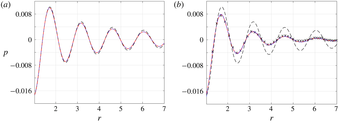
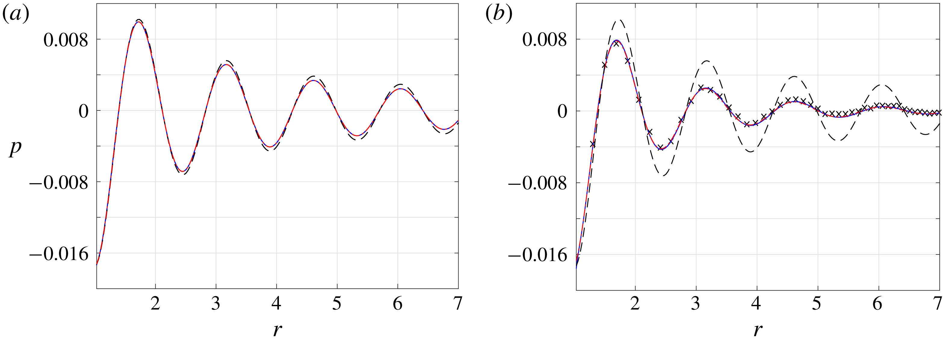
inviscid limit given in (2.6). Towards this end, figure 2 presents the vibroacoustic pressure signal obtained at
 $\unicode[STIX]{x1D714}=4$
and small values of
 $\mathit{Kn}=0.0015$
(figure 2
a) and
 $\mathit{Kn}=0.015$
(figure 2
b). The inviscid solution is shown by the dashed lines for reference. Due to the exceedingly small value of
 $\mathit{Kn}$
in figure 2(a), DSMC results are not presented. In this case, the NSF and R13 solutions coincide, and nearly match with the inviscid result. The effect of gas rarefaction becomes more visible in figure 2(b), where
 $\mathit{Kn}$
is increased by an order of magnitude. While there are still no discrepancies between the NSF and R13 predictions, considerable deviations are observed from the inviscid signal. These are attributed to the added effect of viscosity, which causes a stronger decay rate of the far-field dominating compression wave (see
 $\unicode[STIX]{x1D706}_{1}$
and
 $\unicode[STIX]{x1D706}_{1}^{NSF}$
in (3.15) and (3.20), respectively). The R13 and NSF fields, showing the vanishing of the pressure signal at nearly six radii away from the source, fully agree with the DSMC results depicted by the crosses. This suggests the continuum-limit solution as a viable means for predicting the system behaviour at slightly rarefied conditions, which is particularly useful in view of the relatively slow decay rate of the signal at small
 $\mathit{Kn}$
, and associated exceedingly time consuming DSMC runs.
Breakdown of the continuum inviscid solution with increasing
 $\mathit{Kn}$
for an adiabatic pulsating sphere with
 $\unicode[STIX]{x1D714}=4$
: variation of the pressure fluctuation at (a)
 $\mathit{Kn}=0.0015$
and (b)
 $\mathit{Kn}=0.015$
. The dashed black, solid blue and dash-dotted red curves show the continuum inviscid (
 $\mathit{Kn}\rightarrow 0$
), NSF and R13 results, respectively. The crosses mark DSMC predictions. The results are presented at half-period time,
 $t=T/2=\unicode[STIX]{x03C0}/\unicode[STIX]{x1D714}$
.
The applicability of the NSF and R13 models at higher Knudsen numbers is inspected in figure 3, where both acoustic pressure and radial velocity fields are compared with DSMC computations. The
 $(\mathit{Kn},\unicode[STIX]{x1D714})$
combinations are chosen so that
 $\unicode[STIX]{x1D714}^{2}\mathit{Kn}$
, the leading-order decay rate of the compression wave, is fixed (see
 $\unicode[STIX]{x1D706}_{1}$
and
 $\unicode[STIX]{x1D706}_{1}^{NSF}$
in (3.15) and (3.20), respectively). This is supported by the results, showing that all fields decay at a similar rate away from the source. Recalling that the plots are presented at half-period time, the value of
 $u=-0.02$
at
 $r=1$
agrees with the impermeability condition at the wall, requiring that
 $u=\overline{U}_{w}$
at
 $t=T/2$
.
Applicability of NSF (dashed red lines) and R13 (solid black curves) solutions at non-small (
 ${>}0.1$
) Knudsen numbers and non-large (
 ${\leqslant}1$
) actuation frequencies for an adiabatic pulsating sphere: comparison with DSMC results (crosses) of the (a,c) acoustic pressure and (b,d) radial velocity fields at (a,b)
 $(\mathit{Kn},\unicode[STIX]{x1D714})=(0.125,1)$
and (c,d)
 $(\mathit{Kn},\unicode[STIX]{x1D714})=(0.5,0.5)$
. The results are presented at half-period time,
 $t=T/2=\unicode[STIX]{x03C0}/\unicode[STIX]{x1D714}$
.

Comparing the NSF and R13 results, we observe considerable discrepancies in the higher
 $\mathit{Kn}=0.5$
case in figures 3(c) and 3(d). At this relatively large
 $\mathit{Kn}$
, the effect of the Knudsen-layer mode
 $\unicode[STIX]{x1D706}_{3}$
, missing from the NSF description, becomes dominant, and affects both near- and far-field behaviours. Remarkably, the R13 predictions are in good agreement with DSMC results even at
 $\mathit{Kn}=0.5$
, where the NSF model is ineffective. Our findings therefore establish that, at relatively non-large excitation frequencies (
 $\unicode[STIX]{x1D714}\lesssim 1$
), the R13 model provides results that are applicable at
 $\mathit{Kn}$
values significantly larger than in the NSF scheme. Specifically, for
 $\unicode[STIX]{x1D714}\lesssim 1$
, the calculations indicate that the R13 model is valid up to
 $\mathit{Kn}\approx 0.6$
, while NSF predictions break down already at
 $\mathit{Kn}\approx 0.1$
.
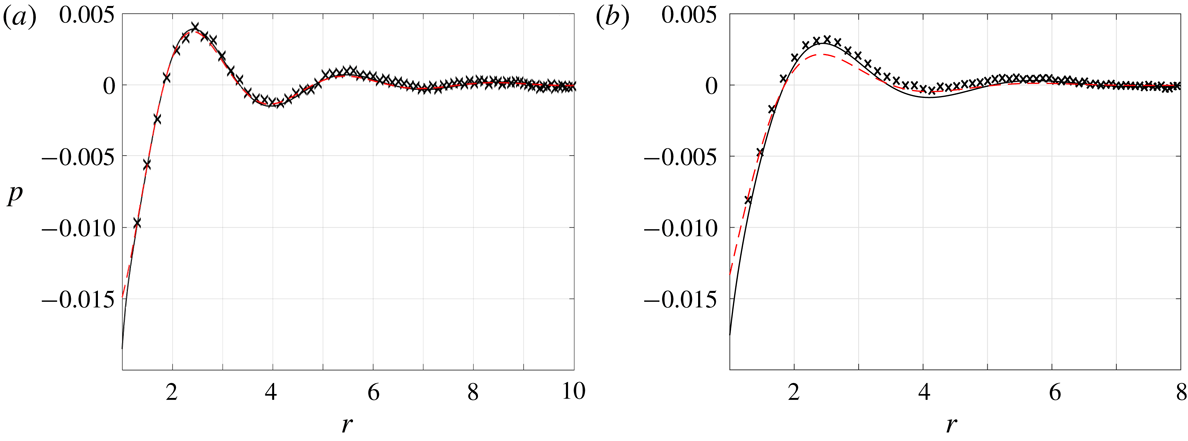
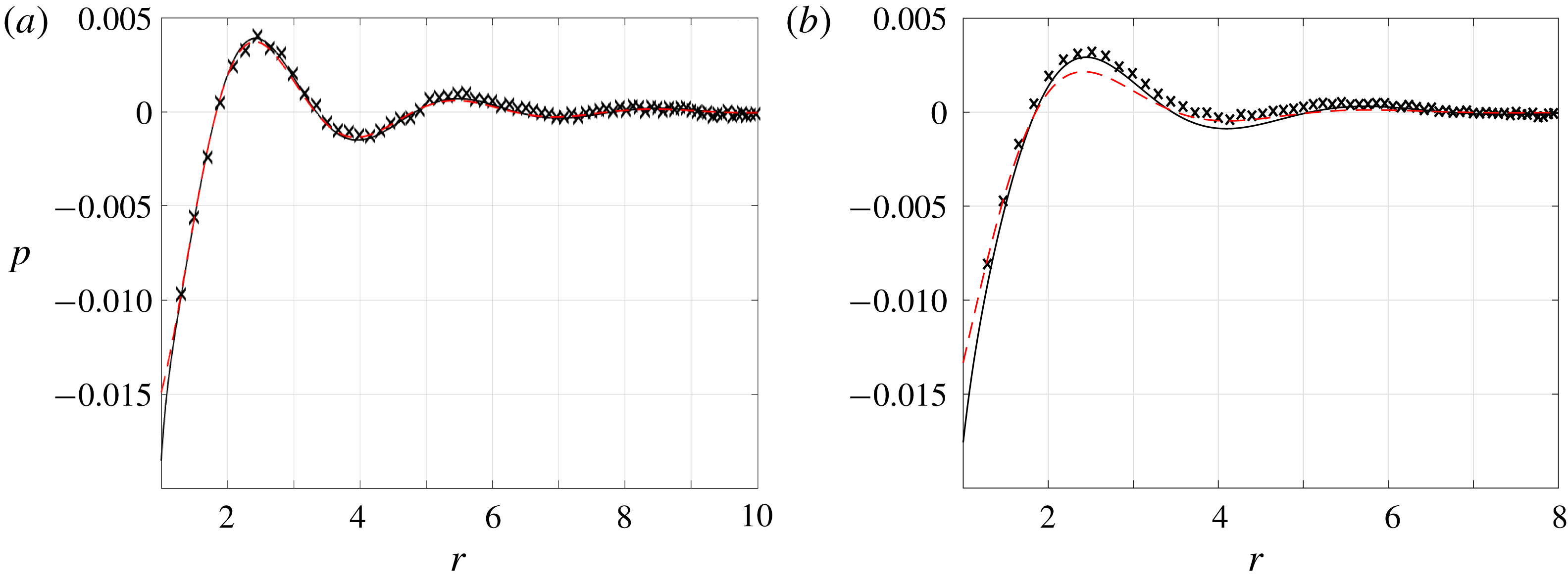
Applicability of NSF (dashed red lines) and R13 (solid black curves) solutions for an adiabatic pulsating sphere with
 $\unicode[STIX]{x1D714}=2$
: comparison of the acoustic pressure with DSMC results (crosses) at (a)
 $\mathit{Kn}=0.06$
and (b)
 $\mathit{Kn}=0.125$
. The results are presented at half-period time,
 $t=T/2=\unicode[STIX]{x03C0}/\unicode[STIX]{x1D714}$
.
Different from the extended applicability of the R13 model at
 $\unicode[STIX]{x1D714}\lesssim 1$
, the scheme does not improve considerably over the NSF description at higher frequencies. In this case, the problem time scale becomes more restrictive in determining the flow regime, and the transition between the near-continuum and intermediate states occurs at lower values of
 $\mathit{Kn}$
. To rationalize the differences between the low- and high-frequency responses, we expand the near-continuum solution obtained in § 3 in
 $\mathit{Kn}$
and
 $\unicode[STIX]{x1D714}$
for
 $r\gg 1$
. Each of the hydrodynamic fields then takes the form
 $$\begin{eqnarray}a_{0}O\left(\frac{\unicode[STIX]{x1D714}}{[1+\unicode[STIX]{x1D714}^{2}/c_{0}^{2}]^{1/2}}\right)+a_{1}O(\unicode[STIX]{x1D714}^{2}\mathit{Kn})+\cdots ,\end{eqnarray}$$
where
 $a_{0}$
and
 $a_{1}$
are independent of
 $\mathit{Kn}$
and
 $\unicode[STIX]{x1D714}$
. The leading-order term represents the inviscid solution (see (2.6)), and the correction originates from the far-field decay of the compression wave (see the
 $\unicode[STIX]{x1D706}_{1}$
component in (3.17)). At
 $\unicode[STIX]{x1D714}\ll 1$
, the leading order is
 $O(\unicode[STIX]{x1D714})$
, which is
 ${\sim}O(\mathit{Kn}_{\unicode[STIX]{x1D714}})$
larger than the
 $O(\unicode[STIX]{x1D714}^{2}\mathit{Kn})$
correction. Since
 $\mathit{Kn}\gg \mathit{Kn}_{\unicode[STIX]{x1D714}}$
at
 $\unicode[STIX]{x1D714}\ll 1$
, the breakdown of the continuum solution is determined by the value of
 $\mathit{Kn}$
. In contrast, for
 $\unicode[STIX]{x1D714}\gg 1$
, the inviscid solution becomes
 $O(1)$
, thus
 ${\sim}O(\unicode[STIX]{x1D714}^{2}\mathit{Kn})$
larger than the correction term. For the near-continuum scheme to be effective it is therefore required that
 $\unicode[STIX]{x1D714}^{2}\mathit{Kn}=\unicode[STIX]{x1D714}\mathit{Kn}_{\unicode[STIX]{x1D714}}\ll 1$
, which restricts the upper limit of Knudsen numbers to decrease as
 $\unicode[STIX]{x1D714}^{-2}$
.
To illustrate the breakdown of the near-continuum scheme at non-small frequencies, figure 4 presents a comparison of the acoustic pressure between the NSF, R13 and DSMC calculations at a fixed
 $\unicode[STIX]{x1D714}=2$
and different values of
 $\mathit{Kn}=0.06$
and
 $\mathit{Kn}=0.125$
. While the NSF and R13 results agree with DSMC data at
 $\mathit{Kn}=0.06$
(corresponding to
 $\unicode[STIX]{x1D714}\mathit{Kn}_{\unicode[STIX]{x1D714}}=0.24$
), they only partially approximate the pressure field at
 $\mathit{Kn}=0.125$
(
 $\unicode[STIX]{x1D714}\mathit{Kn}_{\unicode[STIX]{x1D714}}=0.5$
), with each matching with a different part of the DSMC signal. In line with the above discussion, the results at this and higher values of
 $\unicode[STIX]{x1D714}$
indicate that both the NSF and R13 models break down at an approximately constant value of
 $\unicode[STIX]{x1D714}\mathit{Kn}_{\unicode[STIX]{x1D714}}\approx 0.3$
, with the R13 approximation not providing improvement over the NSF model. This result may be rationalized by recalling that the differences between the schemes are primarily attributed to the Knudsen-layer mode
 $\unicode[STIX]{x1D706}_{3}$
obtained in (3.15), and noting that its decay rate is independent of the excitation frequency (although an increase in
 $\unicode[STIX]{x1D714}$
should inevitably lead to the narrowing of the layer). The apparent deficiency in capturing the system high-frequency behaviour may be resolved by reformulating the R13 equations with account taken of the short characteristic time scales. As most of the existing works on moment equations have focused on steady-flow problems (Torrilhon Reference Torrilhon2016), such an extension has not been followed hitherto, and may be a topic for future investigation.
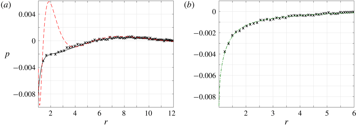
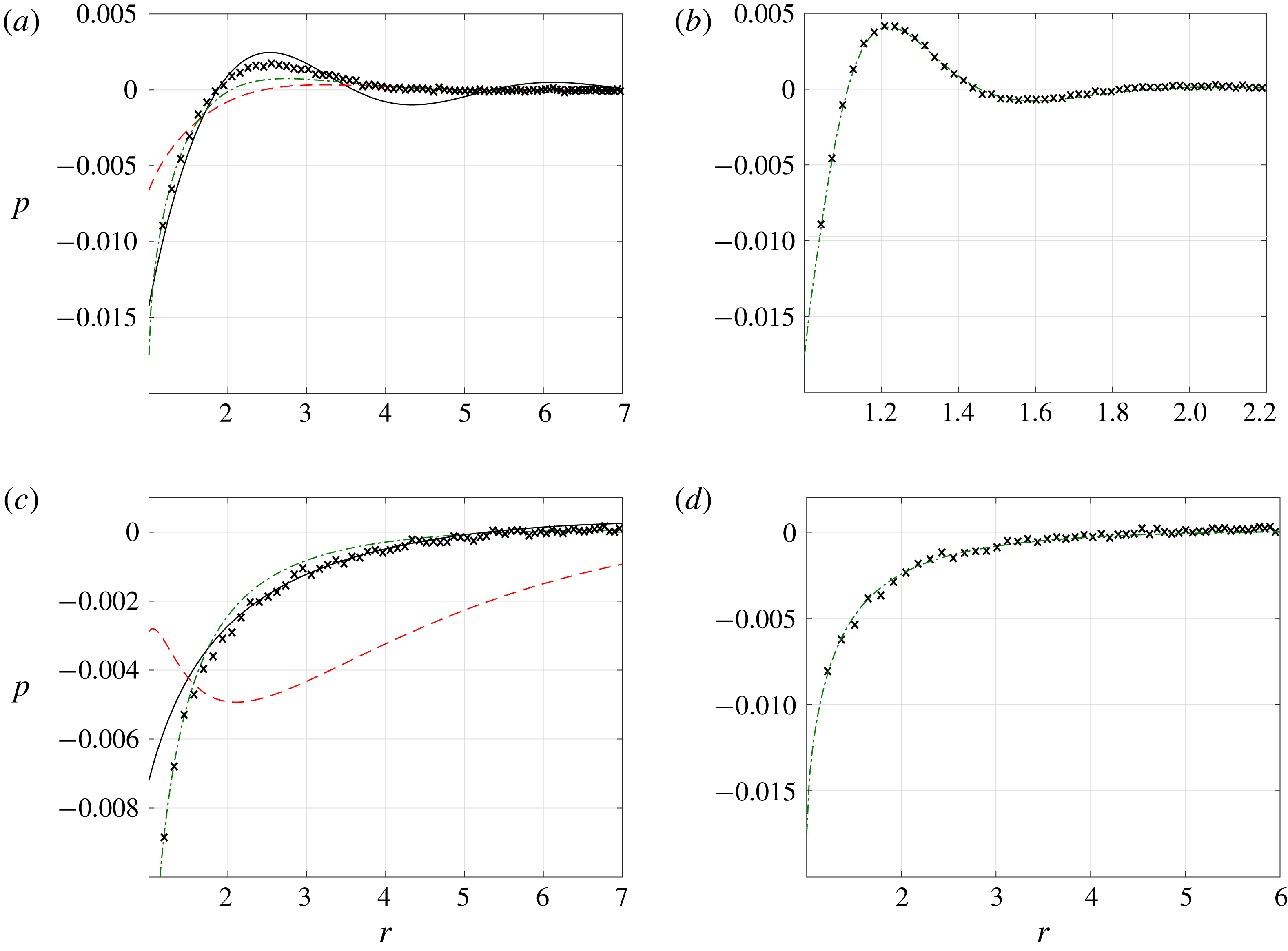
Transition between near-continuum and free-molecular flow regimes for an adiabatic pulsating sphere: comparison between DSMC (crosses), NSF (dashed red lines), R13 (solid black curves) and free-molecular (dash-dotted green lines) solutions for the acoustic pressure at
 $(\mathit{Kn},\unicode[STIX]{x1D714})$
combinations of (a)
 $(0.5,2)$
, (b)
 $(0.5,15)$
, (c)
 $(2,0.5)$
and (d)
 $(6,0.5)$
. The results are presented at half-period time,
 $t=T/2=\unicode[STIX]{x03C0}/\unicode[STIX]{x1D714}$
.
Either by increasing
 $\mathit{Kn}$
above
 ${\approx}0.6$
for
 $\unicode[STIX]{x1D714}\lesssim 1$
, or by taking
 $\unicode[STIX]{x1D714}\mathit{Kn}_{\unicode[STIX]{x1D714}}$
over
 ${\approx}0.3$
for
 $\unicode[STIX]{x1D714}\gtrsim 1$
, the effect of gas rarefaction turns sufficiently strong so that the R13 description breaks down, and the system transits to its intermediate, and, later on, free-molecular regimes. These trends are illustrated in figure 5. As mentioned in the beginning of § 4, free-molecular conditions should prevail wherever the set-up length scale or time scale is short compared with the molecular mean free path or mean free time – or, in terms of the problem non-dimensional parameters,
 $\mathit{Kn}\gg 1$
or
 $\mathit{Kn}_{\unicode[STIX]{x1D714}}\gg 1$
, respectively. These conditions are clearly satisfied by the
 $(\mathit{Kn},\unicode[STIX]{x1D714})$
combinations in figures 5(b) and 5(d), where the free-molecular results agree with DSMC predictions. Intermediate conditions are observed in figures 5(a) and 5(c), where neither the R13, nor ballistic solutions, match with DSMC data. In both figures, the ballistic description provides satisfactory results in the vicinity of the wall (where the effect of molecular collisions is minor), while breaking down at larger
 $r$
.
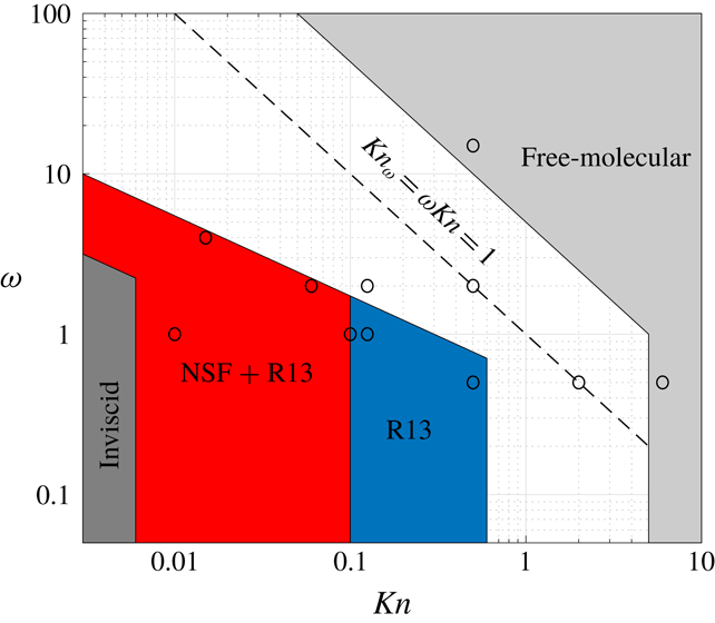
Schematic division of the
 $(\mathit{Kn},\unicode[STIX]{x1D714})$
plane into domains of validity of the inviscid, NSF, R13 and free-molecular descriptions for an adiabatic pulsating sphere. The
 $\mathit{Kn}_{\unicode[STIX]{x1D714}}=1$
line marks the locus of points where the excitation frequency is equal to the collision frequency, and the circles denote the parameter combinations considered in figures 2–5 and 7.
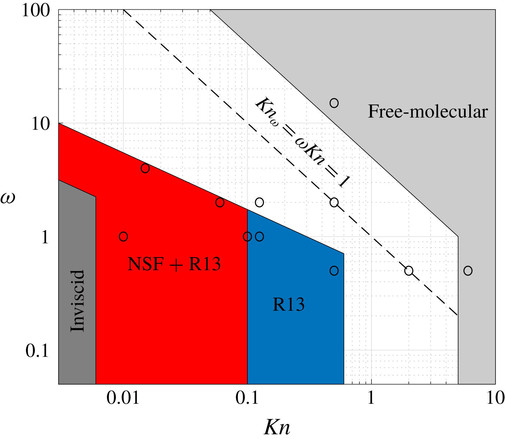
Our discussion on the domains of validity of the approximate solutions is summarized in figure 6, showing a schematic division of the
 $(\mathit{Kn},\unicode[STIX]{x1D714})$
plane into zones where the inviscid, NSF, R13 and free-molecular descriptions prevail. For
 $\unicode[STIX]{x1D714}\lesssim 1$
, corresponding to cases where
 $\mathit{Kn}\gtrsim \mathit{Kn}_{\unicode[STIX]{x1D714}}\gtrsim \unicode[STIX]{x1D714}\mathit{Kn}_{\unicode[STIX]{x1D714}}$
, the acoustic flow regime is governed by
 $\mathit{Kn}$
. Here, the inviscid description breaks down at
 $\mathit{Kn}\approx 0.006$
, whereas the NSF model holds up to
 $\mathit{Kn}\approx 0.1$
. The R13 equations remain effective for
 $\mathit{Kn}\lesssim 0.6$
, above which intermediate flow conditions prevail. The free-molecular limit takes place for
 $\mathit{Kn}\gtrsim 5$
. Considering cases where
 $\unicode[STIX]{x1D714}\gtrsim 1$
(
 $\mathit{Kn}\lesssim \mathit{Kn}_{\unicode[STIX]{x1D714}}\lesssim \unicode[STIX]{x1D714}\mathit{Kn}_{\unicode[STIX]{x1D714}}$
), system rarefaction is governed by the time-scale-based parameters
 $\mathit{Kn}_{\unicode[STIX]{x1D714}}$
and
 $\unicode[STIX]{x1D714}\mathit{Kn}_{\unicode[STIX]{x1D714}}$
. Here, our calculations indicate that the inviscid approximation breaks down above
 $\unicode[STIX]{x1D714}\mathit{Kn}_{\unicode[STIX]{x1D714}}\approx 0.03$
(see figure 2), while the NSF and R13 models turn invalid at a common
 $\unicode[STIX]{x1D714}\mathit{Kn}_{\unicode[STIX]{x1D714}}\approx 0.3$
. The free-molecular regime becomes effective for
 $\mathit{Kn}_{\unicode[STIX]{x1D714}}\gtrsim 5$
.
Variation with
 $r$
of the time-averaged acoustic power
 $\bar{\unicode[STIX]{x1D6F1}}$
for an adiabatic pulsating sphere with
 $\unicode[STIX]{x1D714}=1$
and the indicated values of
 $\mathit{Kn}$
. The dashed lines show the continuum inviscid (
 $\mathit{Kn}\rightarrow 0$
) and free-molecular (
 $\mathit{Kn}\rightarrow \infty$
) limits, whereas the
 $\mathit{Kn}=0.01$
and
 $\mathit{Kn}=0.1$
curves are obtained from the R13 solution.
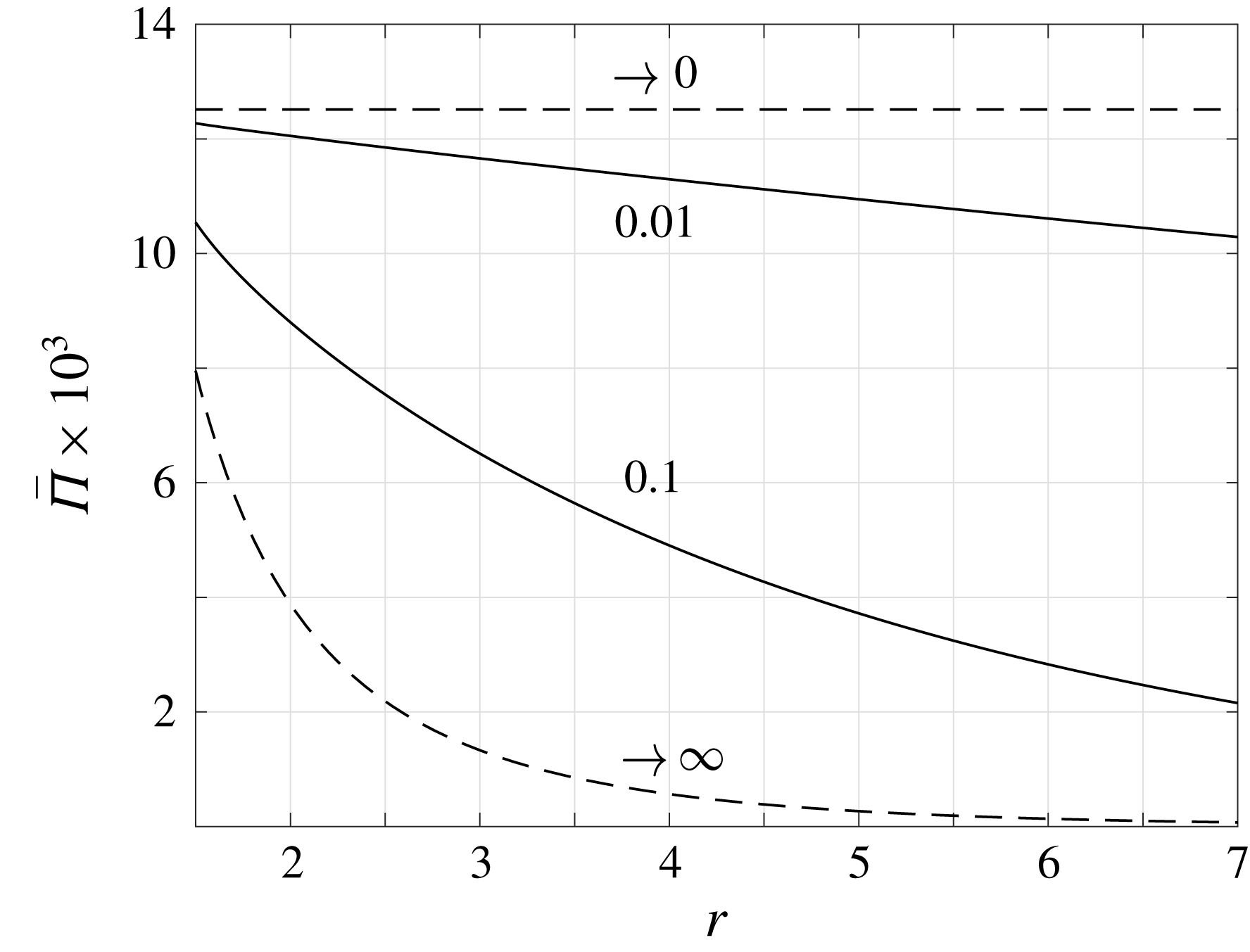
To measure the impact of gas rarefaction on the total source strength, figure 7 presents the effect of the Knudsen number on the time-averaged acoustic power
 $\bar{\unicode[STIX]{x1D6F1}}$
introduced in (2.8). The figure shows the variation of
 $\bar{\unicode[STIX]{x1D6F1}}$
with
 $r$
for
 $\unicode[STIX]{x1D714}=1$
and the indicated values of
 $\mathit{Kn}$
. The asymptotic inviscid (
 $\mathit{Kn}\rightarrow 0$
) and free-molecular (
 $\mathit{Kn}\rightarrow \infty$
) limits are depicted by the dashed lines.
Starting with the inviscid limit, the upper dashed horizontal line in figure 7 shows the far-field
 $r$
-independent result obtained in (2.9). Any viscous effects, manifested by an increase in gas rarefaction, then result in a decrease in the source strength, and in the vanishing of
 $\bar{\unicode[STIX]{x1D6F1}}(r)$
in the far field. At relatively small
 $\mathit{Kn}$
, this stems from the stronger than
 $1/r$
decay rate of both acoustic pressure and radial velocity, formulated by the exponential
 $\unicode[STIX]{x1D706}_{1}$
decline of the compression wave in (3.17). With further increasing
 $\mathit{Kn}$
, the acoustic power reduces at a stronger rate away from the source, until in the free-molecular limit it essentially vanishes at
 $r\approx 7$
. At a given
 $\mathit{Kn}$
, the effective distance where
 $\bar{\unicode[STIX]{x1D6F1}}(r)\rightarrow 0$
diminishes with
 $\unicode[STIX]{x1D714}$
. The results for
 $\bar{\unicode[STIX]{x1D6F1}}(r)$
may be useful in estimating the impact of gas rarefaction on the layer affected by a three-dimensional monopole source.
6.2 Heated stationary sphere
We now consider the thermoacoustic problem of a heated stationary surface. Setting
 $\overline{U}_{w}=0$
and
 $\overline{Q}_{w}=0.02$
, we first validate the applicability of our approximate solutions by comparison with DSMC data. We then examine the possibility of applying boundary heating to cancel out the vibroacoustic sound caused by wall pulsations. Since most of the results are qualitatively similar to those presented in § 6.1, we focus our presentation on findings that have not been previously discussed.
Applicability of NSF (dashed red line), R13 (solid black curve) and free-molecular (dash-dotted green line) solutions for a heated stationary sphere: comparison of the acoustic pressure with DSMC predictions (crosses) at
 $\unicode[STIX]{x1D714}=0.5$
and (a)
 $\mathit{Kn}=0.2$
, (b)
 $\mathit{Kn}=6$
. The results are presented at half-period time,
 $t=T/2=\unicode[STIX]{x03C0}/\unicode[STIX]{x1D714}$
.
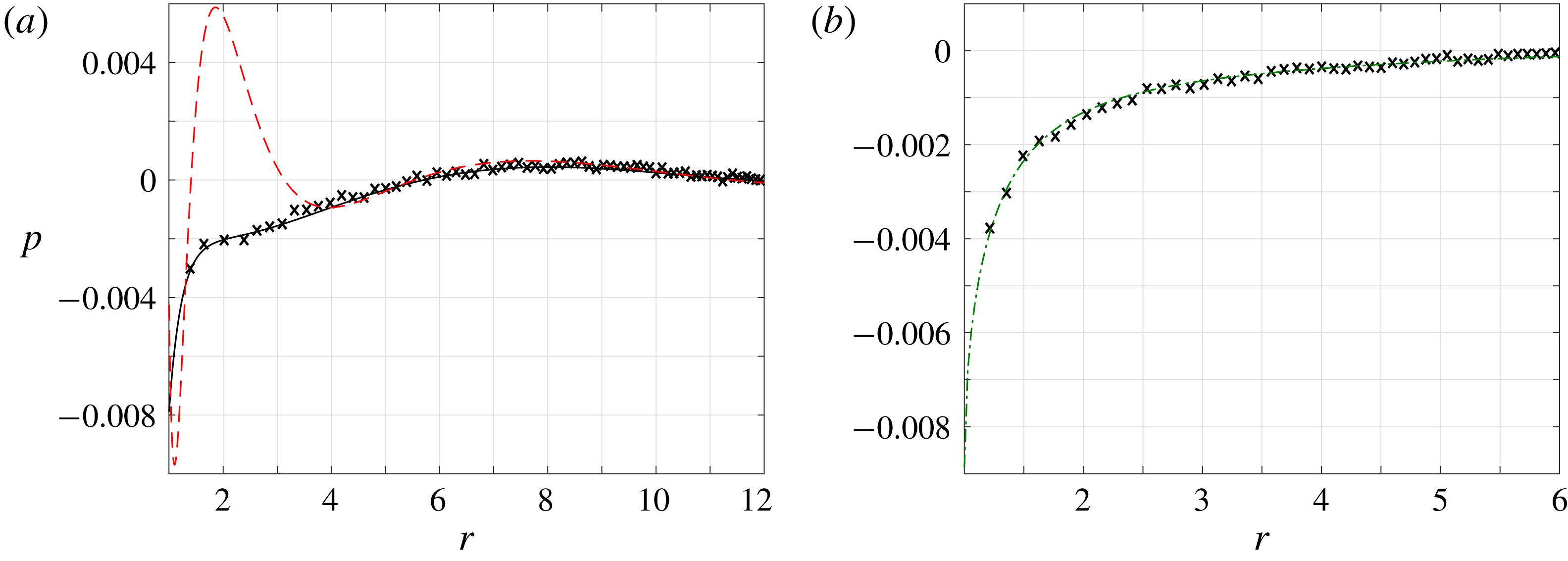
Figure 8 studies the validity of the NSF, R13 and free-molecular approximations through comparison of the acoustic pressure with DSMC-calculated data. Fixing
 $\unicode[STIX]{x1D714}=0.5$
, different values of
 $\mathit{Kn}=0.2$
and
 $\mathit{Kn}=6$
are presented. In line with the schematic map presented in figure 6, the R13 and free-molecular approximations are effective at the low and high values of
 $\mathit{Kn}$
presented, respectively. The NSF solution is invalid in figure 8(a), as the Knudsen number is too high.
Comparison between the vibroacoustic (black solid lines and crosses) and thermoacoustic (red dashed curves and circles) pressure signals for
 $\unicode[STIX]{x1D714}=4$
and (a)
 $\mathit{Kn}=0.015$
, (b)
 $\mathit{Kn}=2$
. The crosses and circles mark DSMC data, the solid and dashed lines in figure 9(a) present R13 results and the solid and dashed curves in figure 9(b) depict free-molecular approximations. The blue dash-dotted line in figure 9(a) shows the difference between the vibroacoustic and thermoacoustic signals with the latter multiplied by
 $\unicode[STIX]{x1D6FE}/2(\unicode[STIX]{x1D6FE}-1)=5/4$
. The results are presented at half-period time,
 $t=T/2=\unicode[STIX]{x03C0}/\unicode[STIX]{x1D714}$
.
Identifying the qualitatively similar waveforms and decay rates of the vibroacoustic and thermoacoustic signals, it appears of interest to examine the effectiveness of using heating-generated sound to reduce the noise caused by mechanical pulsations. Ideally, a linear combination of boundary heating and vibration would result in a moving boundary that generates no sound. Such an approach was followed in the theoretical investigation of a vibrating plane set-up (Manela & Pogorelyuk Reference Manela and Pogorelyuk2015), which was recently tested in a dedicated experiment combining a thermophone device to generate low-frequency thermoacoustic sound (Julius et al. Reference Julius, Gold, Kleiman, Leizeronok and Cukurel2018). Applying first-law thermodynamic considerations, it was shown that complete far-field sound cancellation may be achieved at continuum conditions if boundary pulsations and heating are applied at opposite phases and an amplitude ratio of
 $$\begin{eqnarray}{\mathcal{R}}_{optimal}=\left|\frac{\overline{Q}_{w}}{\overline{U}_{w}}\right|_{optimal}=\frac{\unicode[STIX]{x1D6FE}}{2(\unicode[STIX]{x1D6FE}-1)}=\frac{5}{4},\end{eqnarray}$$
where
 $\unicode[STIX]{x1D6FE}=5/3$
(Manela & Pogorelyuk Reference Manela and Pogorelyuk2015). At non-continuum conditions, only partial cancellation could be achieved due to the more complex nature of the acoustic signal.
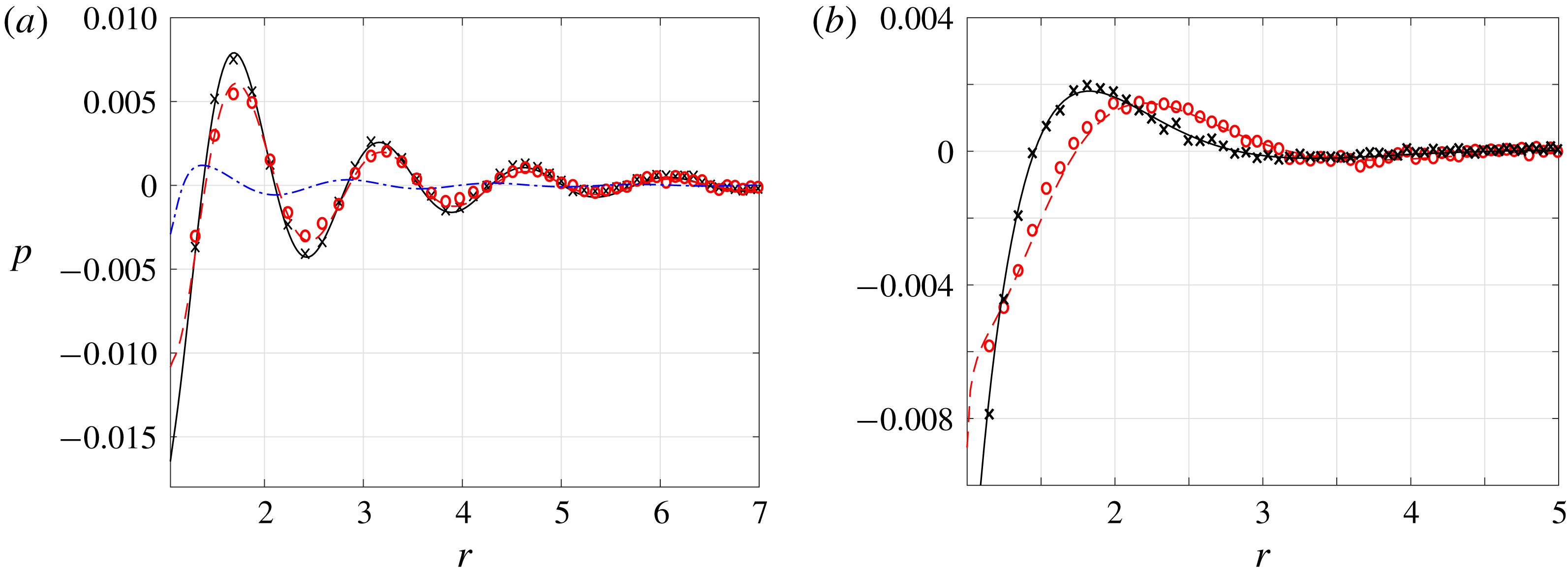
Applying the same approach, figure 9 seeks to test the conditions at which vibroacoustic sound cancellation may be obtained. Since the thermodynamic considerations made in the planar set-up investigation remain unchanged in the spherical configuration, the optimal
 $\unicode[STIX]{x1D6FE}/2(\unicode[STIX]{x1D6FE}-1)$
ratio should hold for
 $\mathit{Kn}\rightarrow 0$
. This is confirmed by the results in figure 9(a), indicating that nearly complete sound cancellation is obtained in the far field at
 $\mathit{Kn}=0.015$
with the above choice of
 ${\mathcal{R}}_{optimal}$
. The non-zero values observed in the vicinity of the boundary (see the dash-dotted blue line in figure 9
a near
 $r=1$
) are mainly attributed to the thermal mode (
 $\unicode[STIX]{x1D706}_{2}$
), which contributes to the near-wall pressure at
 $\mathit{Kn}\neq 0$
. These deviations vanish with further decreasing
 $\mathit{Kn}$
. In contrast, in the limit of large gas rarefaction presented in figure 9(b), the vibroacoustic and thermoacoustic signals appear of different forms, and no single factor multiplication may result in uniform sound cancellation. This is since, at these and other finite Knudsen number conditions, the far-field sound is composed of several acoustic modes, each of which requires different conditions for its cancellation.
7 Conclusion
We studied the vibroacoustic and thermoacoustic responses of a gas to small-amplitude normal-to-boundary mechanical and heat-flux excitations of a sphere at rarefied-flow conditions. The problem was analysed in the entire range of gas rarefaction and input frequencies, to characterize the effect of continuum breakdown on monopole radiation in a three-dimensional set-up. Numerical calculations were carried out via the direct simulation Monte Carlo method, and were used to validate analytical predictions in the free-molecular and near-continuum regimes. In the latter, the regularized thirteen moment (R13) equations were applied, to capture the system response at states where the Navier–Stokes–Fourier (NSF) description breaks down. Comparing with the continuum inviscid solution, the results revealed the dampening effect of gas rarefaction on source point-wise strength and acoustic power. At near-continuum conditions, the acoustic field is composed of exponentially decaying ‘compression’, ‘thermal’ and ‘Knudsen-layer’ modes, reflecting thermoviscous and rarefaction effects. With reducing rarefaction, the contributions of the latter two vanish, and the former mode degenerates into the ideal-flow inverse-to-distance decaying wave. Stronger attenuation was observed with increasing rarefaction, where boundary sphericity results in a ‘geometric reduction’ of the molecular layer affected by the source. Notably, while the R13 model at low frequencies improves over the NSF description at moderate rarefaction levels, both approximations become invalid at common low Knudsen numbers for high frequencies.
While our results have focused on the gas response to harmonic surface excitations, the free-molecular solution in § 4 may be applied for arbitrary small-amplitude input profiles. In addition, the periodic response analysed in the continuum limit may be considered as a generalized Fourier component forming the gas reaction to any time-dependent input. In this context, the frequency-independent value of
 ${\mathcal{R}}_{optimal}$
for sound cancellation, stated in (6.2) and confirmed by figure 9(a), may be of practical value to reduce the vibroacoustic noise generated by any input signal at small Knudsen numbers.
Considering the common breakdown of the NSF and R13 descriptions at high frequencies, it may have been argued that a higher-order moment model (e.g. the regularized twenty-six moment equations, R26 (Gu & Emerson Reference Gu and Emerson2009)) would yield superior results. While this may be true at low frequencies, counterpart improvement is not anticipated at high frequencies. In view of the analysis in § 3, this result may be attributed to the Knudsen-layer mode
 $\unicode[STIX]{x1D706}_{3}$
contained in the R13 solution (see (3.15)), and missing from the NSF description. Here, although an increase in
 $\unicode[STIX]{x1D714}$
should inevitably lead to the narrowing of the layer, the leading order of the mode decay rate is independent of the excitation frequency. Observing that most of the works on moment equations have focused on steady-flow problems, it may therefore be worthwhile to reassess these models in set-ups where short time scales prevail.
Acknowledgements
This research was supported by the Israel Science Foundation (grant no. 1084/16) and the Aeronautical Engineering Research Fund. Y.B. acknowledges the support by the Adams Fellowship Program of the Israel Academy of Sciences and Humanities.
Appendix A. Expressions for the hydrodynamic fields in the R13 solution
In terms of
 $\overline{T}(r)$
, the density amplitude function
 $\overline{\unicode[STIX]{x1D70C}}(r)$
is given by
 $$\begin{eqnarray}\displaystyle \overline{\unicode[STIX]{x1D70C}}(r) & = & \displaystyle \frac{1}{\text{i}\unicode[STIX]{x1D714}\mathit{Kn}\left[1+{\textstyle \frac{61}{5}}\text{i}\unicode[STIX]{x1D714}\mathit{Kn}-{\textstyle \frac{678}{25}}(\unicode[STIX]{x1D714}\mathit{Kn})^{2}+{\textstyle \frac{2016}{25}}\text{i}(\unicode[STIX]{x1D714}\mathit{Kn})^{3}-{\textstyle \frac{2592}{25}}(\unicode[STIX]{x1D714}\mathit{Kn})^{4}\right]}\nonumber\\ \displaystyle & & \displaystyle \times \left\{9\mathit{Kn}^{4}\left[1+{\textstyle \frac{36}{5}}\text{i}\unicode[STIX]{x1D714}\mathit{Kn}\right]^{2}\unicode[STIX]{x1D6FB}_{r}^{4}\overline{T}\right.\nonumber\\ \displaystyle & & \displaystyle -\,{\textstyle \frac{15}{4}}\mathit{Kn}^{2}\left[1+18\text{i}\unicode[STIX]{x1D714}\mathit{Kn}-{\textstyle \frac{2592}{25}}(\unicode[STIX]{x1D714}\mathit{Kn})^{2}-{\textstyle \frac{5184}{25}}\text{i}(\unicode[STIX]{x1D714}\mathit{Kn})^{3}+{\textstyle \frac{93\,312}{625}}(\unicode[STIX]{x1D714}\mathit{Kn})^{4}\right]\unicode[STIX]{x1D6FB}_{r}^{2}\overline{T}\nonumber\\ \displaystyle & & \displaystyle +\left.{\textstyle \frac{3}{2}}\text{i}\unicode[STIX]{x1D714}\mathit{Kn}\left[1+{\textstyle \frac{61}{5}}\text{i}\unicode[STIX]{x1D714}\mathit{Kn}-{\textstyle \frac{1218}{25}}(\unicode[STIX]{x1D714}\mathit{Kn})^{2}-{\textstyle \frac{2448}{25}}\text{i}(\unicode[STIX]{x1D714}\mathit{Kn})^{3}+{\textstyle \frac{2592}{25}}(\unicode[STIX]{x1D714}\mathit{Kn})^{4}\right]\overline{T}\vphantom{\left[{\textstyle \frac{36}{5}}\right]^{2}}\right\}\!.\qquad\end{eqnarray}$$
Assigning
 $\overline{T}(r)$
from (3.17), we find
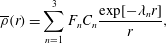 $$\begin{eqnarray}\overline{\unicode[STIX]{x1D70C}}(r)=\mathop{\sum }_{n=1}^{3}F_{n}C_{n}\frac{\exp [-\unicode[STIX]{x1D706}_{n}r]}{r},\end{eqnarray}$$
where
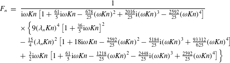 $$\begin{eqnarray}\displaystyle F_{n} & = & \displaystyle \frac{1}{\text{i}\unicode[STIX]{x1D714}\mathit{Kn}\left[1+{\textstyle \frac{61}{5}}\text{i}\unicode[STIX]{x1D714}\mathit{Kn}-{\textstyle \frac{678}{25}}(\unicode[STIX]{x1D714}\mathit{Kn})^{2}+{\textstyle \frac{2016}{25}}\text{i}(\unicode[STIX]{x1D714}\mathit{Kn})^{3}-{\textstyle \frac{2592}{25}}(\unicode[STIX]{x1D714}\mathit{Kn})^{4}\right]}\nonumber\\ \displaystyle & & \displaystyle \times \left\{9(\unicode[STIX]{x1D706}_{n}\mathit{Kn})^{4}\left[1+{\textstyle \frac{36}{5}}\text{i}\unicode[STIX]{x1D714}\mathit{Kn}\right]^{2}\right.\nonumber\\ \displaystyle & & \displaystyle -\,{\textstyle \frac{15}{4}}(\unicode[STIX]{x1D706}_{n}\mathit{Kn})^{2}\left[1+18\text{i}\unicode[STIX]{x1D714}\mathit{Kn}-{\textstyle \frac{2592}{25}}(\unicode[STIX]{x1D714}\mathit{Kn})^{2}-{\textstyle \frac{5184}{25}}\text{i}(\unicode[STIX]{x1D714}\mathit{Kn})^{3}+{\textstyle \frac{93\,312}{625}}(\unicode[STIX]{x1D714}\mathit{Kn})^{4}\right]\nonumber\\ \displaystyle & & \displaystyle +\left.{\textstyle \frac{3}{2}}\text{i}\unicode[STIX]{x1D714}\mathit{Kn}\left[1+{\textstyle \frac{61}{5}}\text{i}\unicode[STIX]{x1D714}\mathit{Kn}-{\textstyle \frac{1218}{25}}(\unicode[STIX]{x1D714}\mathit{Kn})^{2}-{\textstyle \frac{2448}{25}}\text{i}(\unicode[STIX]{x1D714}\mathit{Kn})^{3}+{\textstyle \frac{2592}{25}}(\unicode[STIX]{x1D714}\mathit{Kn})^{4}\right]\vphantom{\left[{\textstyle \frac{36}{5}}\right]^{2}}\!\right\}\end{eqnarray}$$
for
 $n=1,2,3$
. Substituting
 $\overline{\unicode[STIX]{x1D70C}}(r)$
into the continuity equation (3.2), we obtain
 $$\begin{eqnarray}\overline{u}(r)=\text{i}\unicode[STIX]{x1D714}\mathop{\sum }_{n=1}^{3}F_{n}C_{n}\left[\frac{1}{r\unicode[STIX]{x1D706}_{n}}+\frac{1}{(r\unicode[STIX]{x1D706}_{n})^{2}}\right]\exp [-\unicode[STIX]{x1D706}_{n}r].\end{eqnarray}$$
The radial stress amplitude
 $\overline{\unicode[STIX]{x1D70E}}(r)$
is then obtained by substitution of (A 4), together with the linearized form of the equation of state in (3.5), into the
 $r$
-momentum equation (3.3). This yields
 $$\begin{eqnarray}\overline{\unicode[STIX]{x1D70E}}(r)=-\frac{1}{2}\mathop{\sum }_{n=1}^{3}C_{n}\left[1+\left(1+\frac{2\unicode[STIX]{x1D714}^{2}}{\unicode[STIX]{x1D706}_{n}^{2}}\right)F_{n}\right]\left[\frac{1}{r}+\frac{3}{r^{2}\unicode[STIX]{x1D706}_{n}}+\frac{3}{r^{3}\unicode[STIX]{x1D706}_{n}^{2}}\right]\exp [-\unicode[STIX]{x1D706}_{n}r].\end{eqnarray}$$
The heat-flux amplitude
 $\overline{q}(r)$
is calculated from the energy balance (3.4), giving
 $$\begin{eqnarray}\overline{q}(r)=-\frac{1}{2}\text{i}\unicode[STIX]{x1D714}\mathop{\sum }_{n=1}^{3}C_{n}\left(F_{n}-\frac{3}{2}\right)\left[\frac{1}{r\unicode[STIX]{x1D706}_{n}}+\frac{1}{(r\unicode[STIX]{x1D706}_{n})^{2}}\right]\exp [-\unicode[STIX]{x1D706}_{n}r].\end{eqnarray}$$
The constants
 $C_{1,2,3}$
are determined through the boundary conditions (3.10) and (3.11).
Appendix B. Evaluation of
 $I_{n}^{(m)},J_{n}^{(m)}$
and
$K_{n}^{(m)}$
in (4.18)


Substituting (4.13) together with (2.1)–(2.2) in their scaled forms into (4.18),
 $J_{n}^{(1)}$
and
 $K_{n}^{(1)}$
contain a double integral of the form
 $$\begin{eqnarray}J_{n}^{(1)},K_{n}^{(1)}=Re\left\{\frac{1}{\sqrt{\unicode[STIX]{x03C0}}}\exp [i\unicode[STIX]{x1D714}t]\int _{0}^{\unicode[STIX]{x1D702}}\,\text{d}\unicode[STIX]{x1D717}_{\unicode[STIX]{x1D709}}\int _{0}^{\infty }\unicode[STIX]{x1D709}^{n}\sin \unicode[STIX]{x1D717}_{\unicode[STIX]{x1D709}}\exp [-\text{i}\unicode[STIX]{x1D714}x_{w}(r,\unicode[STIX]{x1D717}_{\unicode[STIX]{x1D709}})/\unicode[STIX]{x1D709}-\unicode[STIX]{x1D709}^{2}]\,\text{d}\unicode[STIX]{x1D709}\right\}\!.\end{eqnarray}$$
Focusing on a high-frequency
 $\unicode[STIX]{x1D714}(r-1)\gg 1$
limit and considering the final time-periodic state of the system, the method of steepest descent may be applied to evaluate the
 $\unicode[STIX]{x1D709}$
-integral (Abramowitz Reference Abramowitz1953). This yields
 $$\begin{eqnarray}J_{n}^{(1)},K_{n}^{(1)}\approx Re\left\{3^{-(1+n)/2}\exp [\text{i}\unicode[STIX]{x1D714}t]\int _{0}^{\unicode[STIX]{x1D702}}z^{n/2}\left(1+\frac{a_{1}}{z}+\frac{a_{2}}{z^{2}}+O(z^{-3})\right)\sin \unicode[STIX]{x1D717}_{\unicode[STIX]{x1D709}}\exp [-z]\,\text{d}\unicode[STIX]{x1D717}_{\unicode[STIX]{x1D709}}\right\}\!,\end{eqnarray}$$
where
 $z=3[\unicode[STIX]{x1D714}x_{w}(r,\unicode[STIX]{x1D717}_{\unicode[STIX]{x1D709}})/2]^{2/3}\exp [\text{i}\unicode[STIX]{x03C0}/3]\propto [\unicode[STIX]{x1D714}(r-1)]^{2/3}\gg 1$
, and
 $$\begin{eqnarray}a_{1}=(3n^{2}+3n-1)/12\quad \text{and}\quad a_{2}=(9n^{4}+6n^{3}-51n^{2}-24n+25)/288.\end{eqnarray}$$
Applying the method of stationary phase to estimate the
 $\unicode[STIX]{x1D717}_{\unicode[STIX]{x1D709}}$
-integral about the stationary phase point
 $\unicode[STIX]{x1D717}_{\unicode[STIX]{x1D709}}=0$
, we find
 $$\begin{eqnarray}\displaystyle & & \displaystyle \int _{0}^{\unicode[STIX]{x1D702}}z^{n/2}\left(1+\frac{a_{1}}{z}+\frac{a_{2}}{z^{2}}\right)\sin \unicode[STIX]{x1D717}_{\unicode[STIX]{x1D709}}\exp [-z]\,\text{d}\unicode[STIX]{x1D717}_{\unicode[STIX]{x1D709}}\nonumber\\ \displaystyle & & \displaystyle \quad \approx z_{0}^{n/2}\left(1+\frac{a_{1}}{z_{0}}+\frac{a_{2}}{z_{0}^{2}}\right)\left\{\frac{3}{2rz_{0}}\left[1-e^{-(z_{0}r/3)\unicode[STIX]{x1D702}^{2}}(1+O(\unicode[STIX]{x1D702}^{2}))\right]\right\}\exp [-z_{0}],\end{eqnarray}$$
with
 $z_{0}=3[\unicode[STIX]{x1D714}(r-1)/2]^{2/3}\exp [\text{i}\unicode[STIX]{x03C0}/3]\gg 1$
, which completes the evaluation of
 $J_{n}^{(1)}$
and
 $K_{n}^{(1)}$
in (B 2). It is easily verified that
 $$\begin{eqnarray}(J_{n}^{(2)},K_{n}^{(2)})\approx 2(J_{n}^{(1)},K_{n}^{(1)}),\end{eqnarray}$$
and that the term
 $\sqrt{1-r^{2}\sin ^{2}\unicode[STIX]{x1D717}_{\unicode[STIX]{x1D709}}}$
appearing in
 $I_{n}^{(m)}$
may be approximated by unity for the leading-order evaluation, to yield
 $$\begin{eqnarray}I_{n}^{(m)}\approx J_{n}^{(m)}\approx K_{n}^{(m)}.\end{eqnarray}$$
The approximate expressions in (4.21) for
 $I_{n}^{(m)}$
,
 $J_{n}^{(m)}$
and
 $K_{n}^{(m)}$
then follow.