1 Introduction
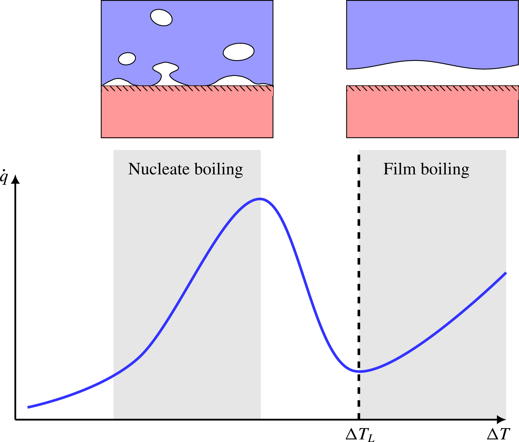
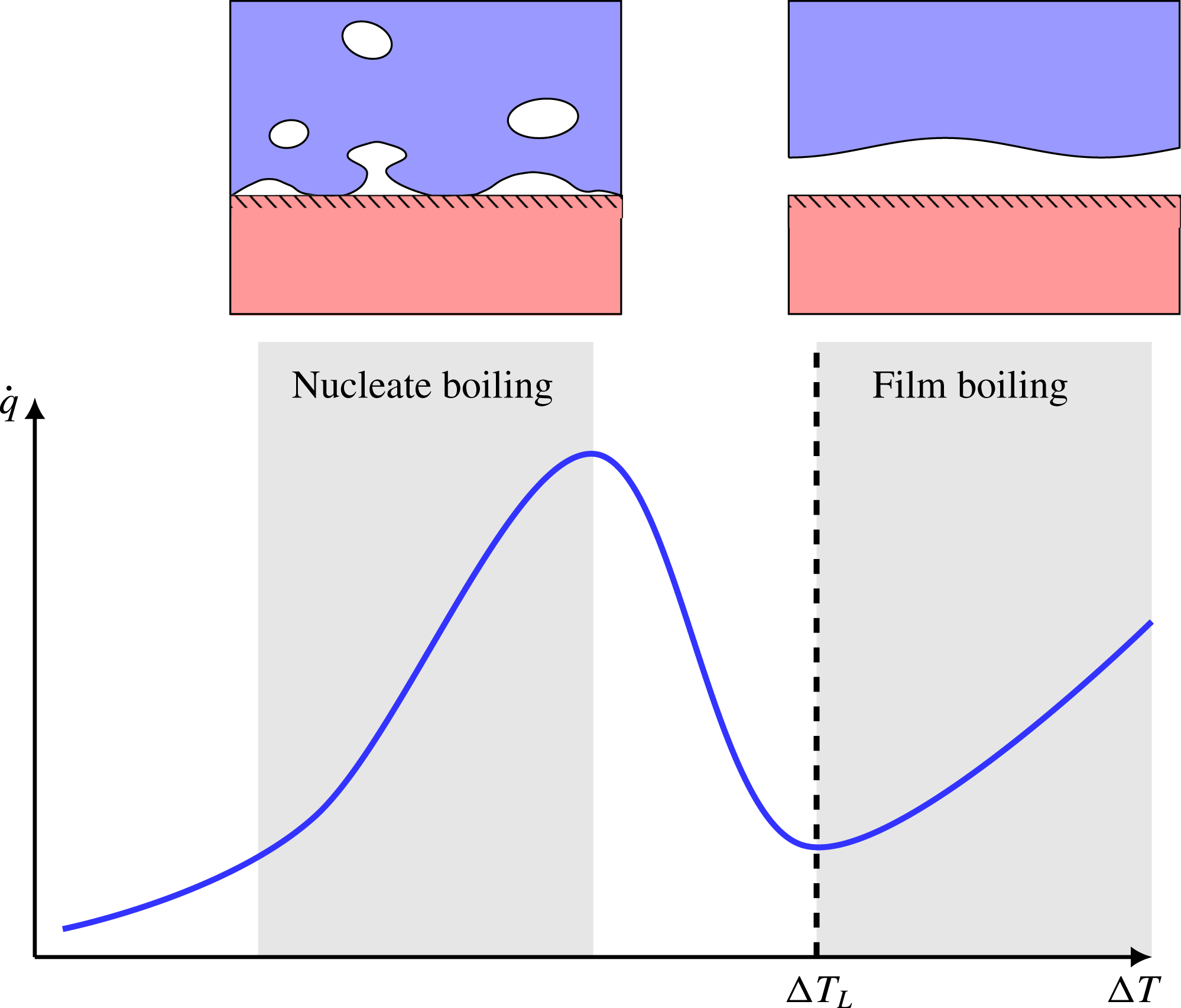
When a liquid is poured on top of a solid surface whose temperature is significantly above the liquid’s saturation temperature, the liquid will start to boil. If we plot the resulting heat flux as a function of surface temperature, we obtain the well-known boiling curve (Dhir Reference Dhir1998), which is illustrated in figure 1. At very high surface temperatures, we get the phenomenon of film boiling, where direct liquid–solid contact is prevented by a continuous sub-millimetre vapour film. This drastically reduces heat transfer compared to the conventional nucleate boiling regime.
An illustration of the boiling curve: a plot of boiling heat flux (
 $\dot{q}$
) against the difference between surface temperature and liquid saturation temperature (
 $\unicode[STIX]{x0394}T$
). At moderate surface temperatures, conventional nucleate boiling occurs, and heat flux is an increasing function of
 $\unicode[STIX]{x0394}T$
. However, at large enough
 $\unicode[STIX]{x0394}T$
, heat flux drops as a transition into the film boiling regime occur. The lowest
 $\unicode[STIX]{x0394}T$
in the film boiling regime is called the Leidenfrost point,
 $\unicode[STIX]{x0394}T_{L}$
.
Of particular importance here is the Leidenfrost point (
 $\unicode[STIX]{x0394}T_{L}$
), also called the minimum film boiling temperature, which is the limiting
 $\unicode[STIX]{x0394}T$
below which film boiling turns unstable. When passing this point from the right, it is called film boiling collapse. Predicting the location of the Leidenfrost point is important for a variety of industrial concerns such as high heat flux cooling applications (e.g. nuclear reactors (Theofanous et al.
Reference Theofanous, Liu, Additon, Angelini, Kymäläinen and Salmassi1997)) and high performance electronics (Agostini et al.
Reference Agostini, Fabbri, Park, Wojtan, Thome and Michel2007), where it is crucial to avoid the film boiling regime in order to keep the heat flux large. Also, film boiling collapse is often believed to be the triggering cause of vapour explosions (rapid phase transition) in nuclear fuel–coolant interactions (Fletcher Reference Fletcher1995; Berthoud Reference Berthoud2000) and liquefied natural gas (LNG) spill incidents (Luketa-Hanlin Reference Luketa-Hanlin2006; Cleaver, Johnson & Ho Reference Cleaver, Johnson and Ho2007). The supposed mechanism behind such vapour explosions is liquid superheating, i.e. the heating of a liquid above its saturation temperature. As we will show, significant superheating at the liquid–vapour interface is only possible if the vapour film becomes very thin, and this is only possible if the uniformly growing solution becomes unstable. Certainly, knowing the value of
 $\unicode[STIX]{x0394}T_{L}$
can be very useful in a variety of applications.
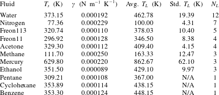
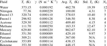
What is known about the Leidenfrost temperature for a given fluid? A lower bound is obviously the saturation temperature. For an upper bound, an empirically supported and physically reasonable value is the liquid spinodal, the temperature beyond which it is thermodynamically impossible for a liquid to be superheated. However, this is quite a large range. For example, water at standard pressure has a saturation temperature of 373 K, while the spinodal can be calculated to be 550 K to 600 K. Measurements of the Leidenfrost point for pools and large droplets of water commonly fall around 460 K (see table 1), but the relative position along the saturation–spinodal interval varies from fluid to fluid.
Fluids for which experimental data on the Leidenfrost temperature could be found. Also shown are the saturation temperature
 $T_{s}$
and the surface tension temperature sensitivity
 $\unicode[STIX]{x1D6FE}$
, found from the NIST database (Linstrom & Mallard Reference Linstrom and Mallard2017; Dean Reference Dean1998). The fourth and fifth columns show the average and standard deviation of the Leidenfrost temperature at atmospheric pressure, based on
 $N_{L}$
data points from the literature. The Leidenfrost temperature data points were found in Berenson (Reference Berenson1961), Gottfried & Bell (Reference Gottfried and Bell1966), Baumeister & Simon (Reference Baumeister and Simon1973), Valencia-Chavez (Reference Valencia-Chavez1978), Yao & Henry (Reference Yao and Henry1978), Sakurai, Shiotsu & Hata (Reference Sakurai, Shiotsu and Hata1990), Nagai & Nishio (Reference Nagai and Nishio1996), Qiao & Chandra (Reference Qiao and Chandra1997), Bernardin & Mudawar (Reference Bernardin and Mudawar1999), Vesovic (Reference Vesovic2007).
There have been a large variety of efforts to pinpoint the Leidenfrost point for any given fluid. Some are based on simplified fluid mechanical considerations, such as the efforts of Zuber (Reference Zuber1959) and Berenson (Reference Berenson1961). Others estimate it by the supposed upper bounds of the spinodal (Spiegler et al. Reference Spiegler, Hopenfeld, Silberberg, Bumpus and Norman1963) or the superheat limit from nucleation theory (Yao & Henry Reference Yao and Henry1978). However, as concluded by Bernardin & Mudawar (Reference Bernardin and Mudawar1999) and in the present work, none of the older models appear to predict in a satisfactory manner the Leidenfrost point for a wide variety of fluids. Also, the ones that are reasonably accurate for conventional fluids are semi-empirical, which provides less physical insight and is dubious for extrapolation to unconventional fluids. Overall, it appears that the underlying mechanism behind film boiling collapse has eluded discovery.
In the present work, we attempt to arrive at a prediction of the Leidenfrost point from the hypothesis that the mechanism behind vapour film collapse is a fluid dynamical instability. The approach is to describe vapour film dynamics through the well-studied long-wave (lubrication) approximation of thin film flow. This approach generally leads to a single scalar highly nonlinear equation for the film-thickness function, and has been thoroughly reviewed by Oron, Davis & Bankoff (Reference Oron, Davis and Bankoff1997), Myers (Reference Myers1998) and Craster & Matar (Reference Craster and Matar2009) for the case of liquid films. However, the present model considers a thin vapour film beneath a liquid bulk and will differ from these well-established models in several ways.
The present work is heavily inspired by two previous works, which both consider thin film flow with phase transition: the model for evaporating liquid films by Burelbach, Bankoff & Davis (Reference Burelbach, Bankoff and Davis1988), and the model for film boiling by Panzarella, Davis & Bankoff (Reference Panzarella, Davis and Bankoff2000). However, while the former includes the thermocapillary effect (Davis Reference Davis1987), liquid films give qualitatively different dynamics than vapour films. On the other hand, while the latter does consider a vapour film, it does not include the thermocapillary effect. The present model is the first to include van der Waals, thermocapillary, vapour thrust and non-equilibrium evaporation effects in the context of film boiling. As will be shown later, the thermocapillary effect will turn out to be crucial, and including it in film boiling is dependent on two model novelties being present:
(i) Non-equilibrium evaporation: in the quasi-equilibrium limit, the interface temperature is locked at the saturation temperature, and no thermocapillary effect is possible. Therefore, it is essential to use a non-equilibrium model, which includes an evaporation-rate-dependent departure from saturation temperature at the interface.
(ii) Non-trivial liquid dynamics: while the liquid velocity far away from the vapour film is assumed to be zero, when there is a non-zero velocity in the vapour the liquid close by will be pulled along to a small degree. However, as we shall show, approximating this by assuming a completely stationary liquid will decouple the model from the thermocapillary effect. It is crucial then to account for the small but non-zero liquid velocity.
The procedure to arrive at the present Leidenfrost model is as follows. In § 2 we set up a flow model for the vapour film, including a van der Waals disjoining pressure, a (linearized) non-equilibrium evaporation model and interface stress conditions that include both vapour thrust (normal stress) and thermocapillary effects (tangential stress). We then apply the long-wave approximation while modelling the effect of liquid pressure and drag to arrive at a single scalar highly nonlinear partial differential equation (PDE) for the dimensionless film thickness.
In § 3 we apply linear stability analysis to the PDE, and arrive at a stability condition for uniform base states. This condition depends on the scale of initial film thickness. We pose the hypothesis that film boiling collapse occurs when the film is unstable for any choice of film-thickness scale, and follow that to its logical conclusion, which turns out to be a theoretical prediction for the Leidenfrost point. This expression suggests that the mechanism for film boiling collapse is that the thermocapillary instability becomes stronger than vapour thrust stabilization. This is a claim that to our knowledge has not been stated previously.
In § 4 we compare with experimental Leidenfrost measurements for 11 different fluids and find decent predictive capabilities for all of them. As we then show in § 5, the most common existing models/correlations are unable to perform as well, especially for the more unusual fluids such as cryogens and liquid metals.
We go on in § 6 to discuss the benefits of this new model, as well as the problem of the unknown evaporation coefficient from kinetic theory. We summarize in § 7, and suggest how the validity of the hypothesis could be proved (or disproved) by further experiments.
2 Model
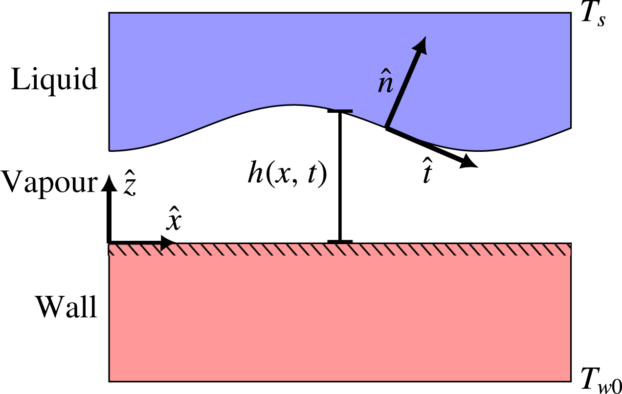
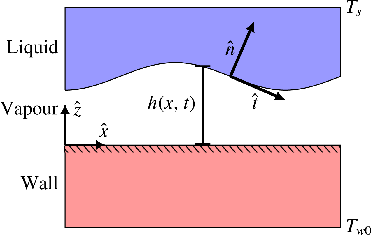
We consider the case of two-dimensional saturated film boiling on a horizontal solid plane, as illustrated in figure 2. The spatial coordinates
 $x$
and
 $z$
run parallel and perpendicular to the plane, respectively. The purpose of the analysis is to predict the dynamics of the film-thickness function,
 $z=h(x,t)$
, where
 $t$
is the time.
Illustration of the physical situation to be modelled. On one side is a liquid whose bulk is held at its saturation temperature. On the other side is a solid slab whose bulk is held at a considerably higher temperature.
 $T_{w0}$
and
 $T_{s}$
are the only given temperatures in this case, and the remaining temperature profile comes from a solution to the problem. The overall temperature difference is
 $\unicode[STIX]{x0394}T$
, and if it is large enough, it will lead to film boiling, i.e. a continuous thin vapour film between the two bulk phases. The general purpose of this model is to predict the dynamics of the liquid–vapour interface, located at
 $z=h(x,t)$
.
2.1 Governing equations of vapour flow
The vapour has velocity components
 $u$
and
 $w$
, in the
 $x$
and
 $z$
directions, respectively. Viscosity (
 $\unicode[STIX]{x1D707}_{v}$
), density (
 $\unicode[STIX]{x1D70C}_{v}$
), thermal conductivity (
 $k_{v}$
) and heat capacity (
 $c_{p,v}$
) are all assumed constant. The governing equations for the vapour flow are the standard continuity, momentum and energy equations for incompressible flow (Kundu, Cohen & Dowling Reference Kundu, Cohen and Dowling2007),
 $$\begin{eqnarray}\displaystyle & \displaystyle u_{x}+w_{z}=0, & \displaystyle\end{eqnarray}$$
 $$\begin{eqnarray}\displaystyle & \displaystyle \unicode[STIX]{x1D70C}_{v}(u_{t}+uu_{x}+wu_{z})=-p_{x}+\unicode[STIX]{x1D707}_{v}(u_{xx}+u_{zz})-\unicode[STIX]{x1D719}_{x}, & \displaystyle\end{eqnarray}$$
 $$\begin{eqnarray}\displaystyle & \displaystyle \unicode[STIX]{x1D70C}_{v}(w_{t}+uw_{x}+ww_{z})=-p_{z}+\unicode[STIX]{x1D707}_{v}(w_{xx}+w_{zz})-\unicode[STIX]{x1D719}_{z}, & \displaystyle\end{eqnarray}$$
 $$\begin{eqnarray}\displaystyle & \displaystyle \unicode[STIX]{x1D70C}_{v}c_{p,v}(T_{t}+uT_{x}+wT_{z})=k_{v}(T_{xx}+T_{zz}), & \displaystyle\end{eqnarray}$$
where variable subscripts imply differentiation. Here
 $p$
is the pressure and
 $\unicode[STIX]{x1D719}$
is the body-force potential. The only difference from standard flow equations so far is that
 $\unicode[STIX]{x1D719}$
includes not only the gravity contribution, but also a film-thickness-dependent addition that represents van der Waals interactions between the liquid surface and the solid surface. This is called a disjoining pressure (Oron et al.
Reference Oron, Davis and Bankoff1997), and gives a total potential of the form
 $$\begin{eqnarray}\displaystyle \unicode[STIX]{x1D719}=\unicode[STIX]{x1D719}_{0}+\unicode[STIX]{x1D70C}_{v}gbz+{\displaystyle \frac{\tilde{A}}{6\unicode[STIX]{x03C0}h^{3}}}. & & \displaystyle\end{eqnarray}$$
Here
 $g$
is the gravitational acceleration, and
 $\tilde{A}$
is the effective Hamaker constant from van der Waals interaction theory. The constant
 $b=\pm 1$
is
 $+1$
for the liquid-above-solid configuration and
 $-1$
for the solid-above-liquid configuration. The constant
 $\unicode[STIX]{x1D719}_{0}$
is an arbitrary reference potential. The van der Waals interaction will only become significant on the sub-micrometre scale of film thickness. A derivation of the last term in (2.5) for the case of thin liquid films can be found in the work of Ruckenstein & Jain (Reference Ruckenstein and Jain1974), and here we assume that a term of the same form is valid for thin vapour films. Generally, the interaction may be either attractive (
 $\tilde{A}>0$
) or repulsive (
 $\tilde{A}<0$
).
2.2 Evaporation model
Due to the high temperature of the solid, evaporation occurs at the liquid–vapour interface, giving an evaporation heat flux
 $j$
. The only given temperatures are the controlled temperature in the solid bulk,
 $T_{w0}$
, and the saturation temperature known from thermodynamics,
 $T_{s}$
. The wall surface temperature,
 $T_{w}$
, will generally be a bit lower than
 $T_{w0}$
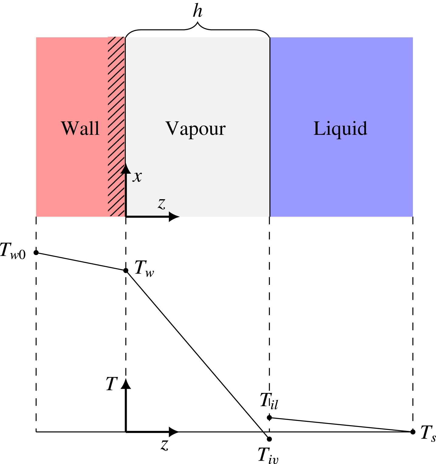
due to the finite thermal conductivity of the solid. Still, the temperature will be continuous at the wall. The situation at the liquid–vapour interface is more complicated. Classically, in the quasi-equilibrium limit, the interface temperature is assumed to be continuous and equal to
 $T_{s}$
. However, generally there is a temperature discontinuity at the interface, and neither side is necessarily equal to
 $T_{s}$
. However, they will both approach
 $T_{s}$
in the limit of weak evaporation. This situation is illustrated in figure 3.
Illustration of the local temperature profile in film boiling, on
 $x$
-scales much shorter than the wavelength seen in figure 2, so that the interface appears flat.

We label the vapour-side and liquid-side interface temperatures as
 $T_{iv}$
and
 $T_{il}$
, respectively. When evaporating, we always have that
 $T_{il}>T_{s}$
and
 $T_{il}>T_{iv}$
. The interface vapour temperature
 $T_{iv}$
may either be below
 $T_{s}$
(supersaturated) or above
 $T_{s}$
(superheated), depending on conditions (Ytrehus Reference Ytrehus1997). For moderate evaporation rates, we may neglect the effect of the discontinuity and consider a single interface temperature,
 $T_{i}=T_{il}\approx T_{iv}$
, which is superheated (
 $T_{i}>T_{s}$
). In these cases we may linearize the relationship between evaporation mass flux and
 $T_{i}$
of the form
 $$\begin{eqnarray}\displaystyle T_{i}-T_{s}=\tilde{K}j, & & \displaystyle\end{eqnarray}$$
as used by Burelbach et al. (Reference Burelbach, Bankoff and Davis1988). The interfacial thermal resistance can be estimated from kinetic gas theory and typically has the form
 $$\begin{eqnarray}\displaystyle \tilde{K}={\displaystyle \frac{\sqrt{2\unicode[STIX]{x03C0}R_{s}}T_{s}^{3/2}}{f(\unicode[STIX]{x1D6FC}_{e})\unicode[STIX]{x1D70C}_{v,s}L}}, & & \displaystyle\end{eqnarray}$$
where
 $R_{s}$
is the specific gas constant,
 $L$
is the latent heat of evaporation,
 $\unicode[STIX]{x1D70C}_{v,s}$
is the vapour density at the saturation temperature and
 $\unicode[STIX]{x1D6FC}_{e}$
is the evaporation coefficient. The function
 $f(\unicode[STIX]{x1D6FC}_{e})$
depends on the specific model. In the moderate-evaporation limit of the classical Hertz–Knudsen model, (Hertz Reference Hertz1882; Knudsen Reference Knudsen1915), we get
 $$\begin{eqnarray}\displaystyle f(\unicode[STIX]{x1D6FC}_{e})=\unicode[STIX]{x1D6FC}_{e}, & & \displaystyle\end{eqnarray}$$
which is what was used by Burelbach et al. (Reference Burelbach, Bankoff and Davis1988). A more recent refinement of this model is the Schrage formula, whose moderate-evaporation limit yields (Mills Reference Mills1995)
 $$\begin{eqnarray}\displaystyle f(\unicode[STIX]{x1D6FC}_{e})={\displaystyle \frac{\unicode[STIX]{x1D6FC}_{e}}{1-\frac{1}{2}\unicode[STIX]{x1D6FC}_{e}}}. & & \displaystyle\end{eqnarray}$$
Some more advanced evaporation models do exist (Ytrehus Reference Ytrehus1997), but quantitatively they reduce to something very similar to the Schrage formula for low-to-moderate evaporation rates.
Usually these models are stated in terms of density differences, not temperature differences like in the constitutive equation used here. Matching the form (2.6) may be achieved by applying the ideal gas law, linearizing the saturation line by the Clausius–Clapeyron relation and assuming that the differences between
 $T_{il}$
,
 $T_{iv}$
and
 $T_{s}$
are small.
The evaporation coefficient
 $\unicode[STIX]{x1D6FC}_{e}$
is the subject of much uncertainty, debate and active research to this date. It is typically assumed equal to the related condensation coefficient (Ytrehus Reference Ytrehus1997; Cheng et al.
Reference Cheng, Lechman, Plimpton and Grest2011). This unknown coefficient is introduced through a boundary condition in kinetic theory, and cannot be determined from within kinetic theory itself. It represents the probability of an incoming vapour molecule sticking to the liquid, as opposed to reflecting back, and is thus by definition in the range of zero to one. The exact nature of this coefficient appears to be far from settled. Water is the only somewhat well-studied fluid, and even there the experiments show a large scatter from
 $0.1$
to
 $1.0$
, as seen in e.g. Tsuruta & Nagayama (Reference Tsuruta and Nagayama2004, Table 1). Besides experiments, a common way of estimating the coefficient is molecular dynamics simulations (MD). These methods show somewhat more consistent results, and generally give values quite close to unity. Overall, MD simulations from the last decade seem to generally agree on the following trends (Tsuruta & Nagayama Reference Tsuruta and Nagayama2004; Cao, Xie & Sazhin Reference Cao, Xie and Sazhin2011; Cheng et al.
Reference Cheng, Lechman, Plimpton and Grest2011; Xie, Sazhin & Cao Reference Xie, Sazhin and Cao2011; Ishiyama et al.
Reference Ishiyama, Fujikawa, Kurz and Lauterborn2013; Iskrenova & Patnaik Reference Iskrenova and Patnaik2017; Liang, Biben & Keblinski Reference Liang, Biben and Keblinski2017):
(i) For a given fluid, the evaporation/condensation coefficient decreases as liquid temperature is increased.
(ii) As long as the liquid temperature is less than 0.7 times
 $T_{c}$
(critical temperature), we can expect
$\unicode[STIX]{x1D6FC}_{e}\in (0.7,1.0)$
for a considerable variety of fluids.


In the cases considered here the liquid surface temperatures are very close to the saturation temperatures, and every liquid considered here has
 $T_{s}<0.7T_{c}$
. Thus we may expect that
 $\unicode[STIX]{x1D6FC}_{e}\in (0.7,1.0)$
.
2.3 Surface tension model
In order to capture the thermocapillary effect, it is essential to include the temperature dependence of surface tension (
 $\unicode[STIX]{x1D70E}$
). We follow Davis (Reference Davis1987) and model the variation as a linearization around its value at the saturation temperature,
 $\unicode[STIX]{x1D70E}_{0}$
,
 $$\begin{eqnarray}\displaystyle \unicode[STIX]{x1D70E}(T)=\unicode[STIX]{x1D70E}_{0}-\unicode[STIX]{x1D6FE}(T-T_{s}). & & \displaystyle\end{eqnarray}$$
Thus, the factor
 $\unicode[STIX]{x1D6FE}$
is
 $$\begin{eqnarray}\displaystyle \unicode[STIX]{x1D6FE}=-{\displaystyle \frac{\unicode[STIX]{x2202}\unicode[STIX]{x1D70E}}{\unicode[STIX]{x2202}T}}. & & \displaystyle\end{eqnarray}$$
For most liquids,
 $\unicode[STIX]{x1D6FE}$
is positive and often around
 $0.0002~\text{N}~\text{m}^{-1}~\text{K}^{-1}$
. As we shall demonstrate,
 $\unicode[STIX]{x1D6FE}$
will play a crucial role in the prediction of vapour film collapse.
2.4 Boundary conditions
2.4.1 Solid wall
The solid wall at
 $z=0$
is an impermeable no-slip surface. Also, as with any interface, there must be a continuity of energy flux. We represent the heat transfer inside the solid with a heat transfer coefficient
 $\unicode[STIX]{x1D6FC}_{w}$
. Since this is a solid,
 $\unicode[STIX]{x1D6FC}_{w}$
could of course be found from the thermal conductivity and a thermal boundary layer thickness, but for simplicity we keep the factor
 $\unicode[STIX]{x1D6FC}_{w}$
. Given the above, the wall surface boundary conditions are
 $$\begin{eqnarray}\displaystyle & \displaystyle u|_{z=0}=w|_{z=0}=0, & \displaystyle\end{eqnarray}$$
 $$\begin{eqnarray}\displaystyle & \displaystyle \unicode[STIX]{x1D6FC}_{w}(T_{w0}-T_{w})=-k_{v}T_{z}|_{z=0}. & \displaystyle\end{eqnarray}$$
2.4.2 Liquid–vapour interface
The liquid–vapour interface is also no-slip, in the sense that the tangential velocity is continuous. In contrast to the solid surface, fluid may pass into this interface at a rate governed by the evaporation mass flux. The relation between the flow velocity at the interface, the velocity of the interface itself, and the evaporation rate is given by the kinematic boundary condition. Additionally, we must have continuity of stress and energy flux across the interface. Given the above, the interface boundary conditions are
 $$\begin{eqnarray}\displaystyle & \displaystyle (\boldsymbol{v}-\boldsymbol{v}_{l})\boldsymbol{\cdot }\hat{\boldsymbol{t}}|_{z=h}=0, & \displaystyle\end{eqnarray}$$
 $$\begin{eqnarray}\displaystyle & \displaystyle \unicode[STIX]{x1D70C}_{v}{\displaystyle \frac{(h_{t}+uh_{x}-w)|_{z=h}}{\sqrt{1+h_{x}^{2}}}}=j, & \displaystyle\end{eqnarray}$$
 $$\begin{eqnarray}\displaystyle & \displaystyle [j(\boldsymbol{v}_{l,e}-\boldsymbol{v}_{e})\boldsymbol{\cdot }\hat{\boldsymbol{n}}-([\unicode[STIX]{x1D64F}-\unicode[STIX]{x1D64F}_{l}]\boldsymbol{\cdot }\hat{\boldsymbol{n}})\boldsymbol{\cdot }\hat{\boldsymbol{n}}]_{z=h}=-\unicode[STIX]{x1D705}\unicode[STIX]{x1D70E}, & \displaystyle\end{eqnarray}$$
 $$\begin{eqnarray}\displaystyle & \displaystyle ([\unicode[STIX]{x1D64F}-\unicode[STIX]{x1D64F}_{l}]_{z=h}\boldsymbol{\cdot }\hat{\boldsymbol{n}})\boldsymbol{\cdot }\hat{\boldsymbol{t}}=\unicode[STIX]{x1D735}\unicode[STIX]{x1D70E}|_{z=h}\boldsymbol{\cdot }\hat{\boldsymbol{t}}, & \displaystyle\end{eqnarray}$$
 $$\begin{eqnarray}\displaystyle & \displaystyle -k_{v}\unicode[STIX]{x1D735}T\boldsymbol{\cdot }\hat{\boldsymbol{n}}|_{z=h}-\unicode[STIX]{x1D6FC}_{l}(T_{i}-T_{s})=jL. & \displaystyle\end{eqnarray}$$
Here the vectors
 $\boldsymbol{v}=[u,w]$
,
 $\hat{\boldsymbol{n}}$
and
 $\hat{\boldsymbol{t}}$
are the velocity, interface unit normal and interface unit tangent, respectively. The latter two are defined as shown in figure 2. The symbol
 $\unicode[STIX]{x1D705}$
is the interface curvature. The symbol
 $\unicode[STIX]{x1D64F}$
is the incompressible Newtonian flow stress tensor,
 $j$
is the evaporation mass flux, and
 $L$
is the fluid’s latent heat of evaporation. The efficiency of heat transfer from the interface to the liquid bulk is represented by a heat transfer coefficient
 $\unicode[STIX]{x1D6FC}_{l}$
. Overall, the subscript
 $l$
indicates the corresponding property on the liquid side.
2.5 Comparison with some previous models
The inclusion of a disjoining-pressure term in § 2.1 is identical to the treatment in Burelbach et al. (Reference Burelbach, Bankoff and Davis1988), though here presumably with a different value for the Hamaker constant due to the nature of the thin film. Similarly, the constitutive equation for evaporation in § 2.2 is similar, though here with a generalization allowing for different factors
 $f(\unicode[STIX]{x1D6FC}_{e})$
. The model of Burelbach et al. (Reference Burelbach, Bankoff and Davis1988) only uses the older Hertz–Knudsen model (2.8). The linearized surface tension model in § 2.3 is quite standard.
The differences to previous works become more nuanced when it comes to the boundary conditions in § 2.4. At the solid surface, the flow boundary conditions (2.12) are standard. However, an energy flux balance like (2.13) is not included in Burelbach et al. (Reference Burelbach, Bankoff and Davis1988), which simply assumes a constant given wall surface temperature. The interface boundary conditions (2.14)–(2.18) are essentially the same as the ones initially presented in Burelbach et al. (Reference Burelbach, Bankoff and Davis1988, equations (2.6)–(2.12)), besides some subtle sign changes due to the liquid–vapour role reversal. However, in Burelbach et al. (Reference Burelbach, Bankoff and Davis1988), the full boundary conditions are considerably simplified due to the negligible density, viscosity and conductivity of the bulk vapour phase outside the film. This cannot be done here as the outside bulk is liquid, and thus, the boundary conditions must remain in their complex form.
Some of the commonalities missing from Burelbach et al. (Reference Burelbach, Bankoff and Davis1988) are present in Panzarella et al. (Reference Panzarella, Davis and Bankoff2000). The latter considers a vapour film and does allow the solid surface temperature to vary. However, they include neither vapour thrust, thermocapillary nor van der Waals effects. In fact, they take the infinite liquid viscosity limit, which leads to setting the vapour interface velocity to zero. As we shall show, this limit has an important qualitative consequence, as it causes the model to decouple from the thermocapillary effect.
2.6 Scales and dimensionless numbers
We introduce a length scale
 $h_{0}$
for
 $z$
and
 $h$
in order to define the dimensionless equivalents
 $Z$
and
 $H$
. Similarly, we introduce a length scale
 $x_{0}$
for
 $x$
in order to define the dimensionless distance
 $X$
. The scales
 $h_{0}$
and
 $x_{0}$
are not arbitrary, and must be set similar to the typical film-thickness and interface disturbance wavelength, in order to ensure
 $\unicode[STIX]{x2202}/\unicode[STIX]{x2202}X\sim \unicode[STIX]{x2202}/\unicode[STIX]{x2202}Z\sim \mathit{O}(1)$
in the dimensionless equations. Here we choose
 $x_{0}=\unicode[STIX]{x1D706}/(2\unicode[STIX]{x03C0})$
, where
 $\unicode[STIX]{x1D706}$
is the wavelength of the disturbance. The ratio between the two scales is defined as
 $$\begin{eqnarray}\displaystyle \unicode[STIX]{x1D716}={\displaystyle \frac{h_{0}}{x_{0}}}=2\unicode[STIX]{x03C0}{\displaystyle \frac{h_{0}}{\unicode[STIX]{x1D706}}}. & & \displaystyle\end{eqnarray}$$
We shall later take the long-wave approximation, which formally is the limit of small
 $\unicode[STIX]{x1D716}$
, i.e.
 $\unicode[STIX]{x1D706}\gg h_{0}$
. We use a velocity scale
 $u_{0}$
to define the dimensionless tangential velocity,
 $U=u/u_{0}$
. Similarly we define the dimensionless perpendicular velocity
 $W=w/w_{0}$
, where continuity implies that
 $w_{0}=\unicode[STIX]{x1D716}u_{0}$
. The dimensionless time
 $\unicode[STIX]{x1D70F}$
is defined by the time scale
 $x_{0}/u_{0}$
. We scale the temperature according to its position on the scale between
 $T_{w0}$
and
 $T_{s}$
,
 $$\begin{eqnarray}\displaystyle \unicode[STIX]{x1D703}={\displaystyle \frac{T-T_{s}}{\unicode[STIX]{x0394}T}}, & & \displaystyle\end{eqnarray}$$
where
 $\unicode[STIX]{x0394}T=T_{w0}-T_{s}$
. We scale the remaining variables as
 $$\begin{eqnarray}p={\displaystyle \frac{\unicode[STIX]{x1D707}_{v}u_{0}}{\unicode[STIX]{x1D716}h_{0}}}P,\quad \unicode[STIX]{x1D719}={\displaystyle \frac{\unicode[STIX]{x1D707}_{v}u_{0}}{\unicode[STIX]{x1D716}h_{0}}}\unicode[STIX]{x1D6F7},\quad j={\displaystyle \frac{k_{v}\unicode[STIX]{x0394}T}{h_{0}L}}J,\quad \unicode[STIX]{x1D70E}=\unicode[STIX]{x1D70E}_{0}\unicode[STIX]{x1D6F4},\end{eqnarray}$$
where
 $P$
,
 $\unicode[STIX]{x1D6F7}$
,
 $J$
and
 $\unicode[STIX]{x1D6F4}$
are the dimensionless pressure, body-force potential, evaporation mass flux and surface tension, respectively. We define the following dimensionless numbers:
 $$\begin{eqnarray}\displaystyle \left.\begin{array}{@{}c@{}}Re={\displaystyle \frac{\unicode[STIX]{x1D70C}_{v}u_{0}h_{0}}{\unicode[STIX]{x1D707}_{v}}},\quad Pr={\displaystyle \frac{\unicode[STIX]{x1D707}_{v}c_{p,v}}{k_{v}}},\quad \unicode[STIX]{x1D6F9}={\displaystyle \frac{\unicode[STIX]{x1D707}_{v}}{\unicode[STIX]{x1D707}_{l}}},\quad D={\displaystyle \frac{\unicode[STIX]{x1D70C}_{v}}{\unicode[STIX]{x1D70C}_{l}}},\quad E={\displaystyle \frac{k_{v}\unicode[STIX]{x0394}T}{\unicode[STIX]{x1D70C}_{v}u_{0}h_{0}L}},\\ K={\displaystyle \frac{\tilde{K}k_{v}}{h_{0}L}},\quad Ca={\displaystyle \frac{\unicode[STIX]{x1D707}_{v}u_{0}}{\unicode[STIX]{x1D70E}_{0}}},\quad M={\displaystyle \frac{\unicode[STIX]{x0394}T\unicode[STIX]{x1D6FE}}{\unicode[STIX]{x1D707}_{v}u_{0}}},\quad A={\displaystyle \frac{\tilde{A}}{6\unicode[STIX]{x03C0}\unicode[STIX]{x1D707}_{v}u_{0}h_{0}^{2}}},\\ G_{v}={\displaystyle \frac{\unicode[STIX]{x1D70C}_{v}gh_{0}^{2}}{\unicode[STIX]{x1D707}_{v}u_{0}}},\quad G_{l}={\displaystyle \frac{\unicode[STIX]{x1D70C}_{l}gh_{0}^{2}}{\unicode[STIX]{x1D707}_{v}u_{0}}},\quad G={\displaystyle \frac{\unicode[STIX]{x0394}\unicode[STIX]{x1D70C}gh_{0}^{2}}{\unicode[STIX]{x1D707}_{v}u_{0}}},\quad Bi_{w}={\displaystyle \frac{\unicode[STIX]{x1D6FC}_{w}h_{0}}{k_{v}}},\quad Bi_{l}={\displaystyle \frac{\unicode[STIX]{x1D6FC}_{l}h_{0}}{k_{v}}}.\end{array}\right\} & & \displaystyle\end{eqnarray}$$
2.7 Long-wave approximation
2.7.1 Approximate equations
We introduce the scales and dimensionless numbers of § 2.6 and make the assumptions of long waves and small Reynolds number, while retaining surface tension effects to leading order,
 $$\begin{eqnarray}\unicode[STIX]{x1D716}\ll 1,\quad \unicode[STIX]{x1D716}Re\ll 1,\quad D\ll 1,\quad Pr\sim \mathit{O}(1),\quad \unicode[STIX]{x1D716}^{3}Ca^{-1}\sim \mathit{O}(1),\quad \unicode[STIX]{x1D716}M\sim \mathit{O}(1).\quad\end{eqnarray}$$
We also want to retain the vapour thrust, van der Waals and gravitational effects to leading order, so we keep the terms
 $\unicode[STIX]{x1D716}ReE^{2}J^{2}$
,
 $\unicode[STIX]{x1D716}A/H^{3}$
and
 $\unicode[STIX]{x1D716}G_{v}$
. Given this, the governing equations of the vapour flow, equations (2.1)–(2.3) and (2.5) become
 $$\begin{eqnarray}\displaystyle & \displaystyle U_{X}+W_{Z}=0, & \displaystyle\end{eqnarray}$$
 $$\begin{eqnarray}\displaystyle & \displaystyle (P+\unicode[STIX]{x1D6F7})_{X}=U_{ZZ}, & \displaystyle\end{eqnarray}$$
 $$\begin{eqnarray}\displaystyle & \displaystyle (P+\unicode[STIX]{x1D6F7})_{Z}=0, & \displaystyle\end{eqnarray}$$
 $$\begin{eqnarray}\displaystyle & \displaystyle \unicode[STIX]{x1D6F7}=\unicode[STIX]{x1D6F7}_{0}+\unicode[STIX]{x1D716}bG_{v}Z+{\displaystyle \frac{\unicode[STIX]{x1D716}A}{H^{3}}}, & \displaystyle\end{eqnarray}$$
respectively. The boundary conditions of the vapour flow (2.12), (2.14), (2.15), (2.16) and (2.17) become
 $$\begin{eqnarray}\displaystyle & \displaystyle [U]_{Z=0}=[W]_{Z=0}=0, & \displaystyle\end{eqnarray}$$
 $$\begin{eqnarray}\displaystyle & \displaystyle [U-U_{l}]_{Z=H}=0, & \displaystyle\end{eqnarray}$$
 $$\begin{eqnarray}\displaystyle & \displaystyle {\displaystyle \frac{E}{\unicode[STIX]{x1D716}}}J=[H_{\unicode[STIX]{x1D70F}}+UH_{X}-W]_{Z=H}, & \displaystyle\end{eqnarray}$$
 $$\begin{eqnarray}\displaystyle & \displaystyle [P-P_{l}]_{Z=H}+\unicode[STIX]{x1D716}ReE^{2}J^{2}=-H_{XX}\unicode[STIX]{x1D716}^{3}Ca^{-1}, & \displaystyle\end{eqnarray}$$
 $$\begin{eqnarray}\displaystyle & \displaystyle [U_{Z}-\unicode[STIX]{x1D6F9}^{-1}U_{l,Z}]_{Z=H}=-\unicode[STIX]{x1D716}M(\unicode[STIX]{x1D703}_{i})_{X}, & \displaystyle\end{eqnarray}$$
respectively. Similarly, the energy equation (2.4) becomes
 $$\begin{eqnarray}\displaystyle \unicode[STIX]{x1D703}_{ZZ}=0, & & \displaystyle\end{eqnarray}$$
and the temperature boundary conditions (2.6), (2.13) and (2.18) become
 $$\begin{eqnarray}\displaystyle & \displaystyle KJ=\unicode[STIX]{x1D703}_{i}, & \displaystyle\end{eqnarray}$$
 $$\begin{eqnarray}\displaystyle & \displaystyle -\unicode[STIX]{x1D703}_{Z}|_{Z=0}=Bi_{w}(1-\unicode[STIX]{x1D703}_{w}), & \displaystyle\end{eqnarray}$$
 $$\begin{eqnarray}\displaystyle & \displaystyle J=-\unicode[STIX]{x1D703}_{Z}|_{Z=H}-Bi_{l}\unicode[STIX]{x1D703}_{i}, & \displaystyle\end{eqnarray}$$
respectively. The van der Waals effect is included in (2.27) (
 ${\sim}A$
), the vapour thrust effect is included in (2.31) (
 ${\sim}ReE^{2}$
), and the thermocapillary effect is included in (2.32) (
 ${\sim}M$
). These long-wave approximation equations have many similarities to the ones presented in Burelbach et al. (Reference Burelbach, Bankoff and Davis1988, equations (5.5)–(5.10)). However, there are significant differences. Besides some sign changes, these differences all relate to the fact that the bulk phase outside the thin film is different. In Burelbach et al. (Reference Burelbach, Bankoff and Davis1988), the normal-stress condition (here (2.31)) does not include a term for the outside pressure as it could be conveniently set constant and equal to zero. In the tangential-stress condition (here (2.32)), the bulk phase shear rate was set to zero, as the interface could be treated as a free surface. Neither simplification is possible in the present work, as the liquid and vapour have switched places. The equations for the temperature profile are also somewhat more complicated in the present work, since the wall surface temperature is allowed to vary (giving (2.35)) and since the bulk phase conductivity cannot be neglected (giving the final term of (2.36)). Overall, the main difference is that with this problem we cannot make a purely ‘one-sided’ model like in Burelbach et al. (Reference Burelbach, Bankoff and Davis1988).
2.7.2 Solution to temperature equations
We note how (2.33)–(2.36) for the temperature profile have no explicit time dependence, only implicitly through the variables
 $J(X,\unicode[STIX]{x1D70F})$
and
 $H(X,\unicode[STIX]{x1D70F})$
. Since
 $J$
is determined directly from the temperature profile through (2.34), the instantaneous value of
 $H$
determines the current temperature profile
 $\unicode[STIX]{x1D703}$
as well as the evaporation mass flux
 $J$
. The solution is
 $$\begin{eqnarray}\displaystyle & \displaystyle J(H)={\displaystyle \frac{1}{K+(Bi_{w}^{-1}+H)C}}, & \displaystyle\end{eqnarray}$$
 $$\begin{eqnarray}\displaystyle & \displaystyle \unicode[STIX]{x1D703}_{i}(H)={\displaystyle \frac{K}{K+(Bi_{w}^{-1}+H)C}}, & \displaystyle\end{eqnarray}$$
 $$\begin{eqnarray}\displaystyle & \displaystyle \unicode[STIX]{x1D703}_{w}(H)={\displaystyle \frac{K+HC}{K+(Bi_{w}^{-1}+H)C}}, & \displaystyle\end{eqnarray}$$
where we have defined the new constant
 $$\begin{eqnarray}\displaystyle C=1+C^{\prime }. & & \displaystyle\end{eqnarray}$$
Here
 $C^{\prime }=Bi_{l}K=\unicode[STIX]{x1D6FC}_{l}\tilde{K}/L$
and represents the effect of heat lost into the liquid bulk. Interestingly,
 $C^{\prime }$
is independent of
 $h_{0}$
, even though the interface temperature
 $\unicode[STIX]{x1D703}_{i}$
is not. It is instructive to look at a few special cases of this solution. In the quasi-equilibrium limit (
 $K\rightarrow 0$
), we get
 $$\begin{eqnarray}\displaystyle & \displaystyle J(K\rightarrow 0)={\displaystyle \frac{1}{Bi_{w}^{-1}+H}}, & \displaystyle\end{eqnarray}$$
 $$\begin{eqnarray}\displaystyle & \displaystyle \unicode[STIX]{x1D703}_{i}(K\rightarrow 0)=0, & \displaystyle\end{eqnarray}$$
 $$\begin{eqnarray}\displaystyle & \displaystyle \unicode[STIX]{x1D703}_{w}(K\rightarrow 0)={\displaystyle \frac{H}{Bi_{w}^{-1}+H}}. & \displaystyle\end{eqnarray}$$
As expected, the interface temperature is locked to
 $T_{s}$
. The evaporation rate is somewhat limited by the finite conductivity of the solid. If
 $H\rightarrow 0$
,
 $J$
does not diverge, due to the finite solid heat transfer efficiency. In the limit of a perfectly conducting solid (
 $Bi_{w}\rightarrow \infty$
) we get
 $$\begin{eqnarray}\displaystyle & \displaystyle J(Bi_{w}\rightarrow \infty )={\displaystyle \frac{1}{K+HC}}, & \displaystyle\end{eqnarray}$$
 $$\begin{eqnarray}\displaystyle & \displaystyle \unicode[STIX]{x1D703}_{i}(Bi_{w}\rightarrow \infty )={\displaystyle \frac{K}{K+HC}}, & \displaystyle\end{eqnarray}$$
 $$\begin{eqnarray}\displaystyle & \displaystyle \unicode[STIX]{x1D703}_{w}(Bi_{w}\rightarrow \infty )=1. & \displaystyle\end{eqnarray}$$
As expected, the wall surface temperature is locked to the bulk temperature,
 $T_{w0}$
. The evaporation rate is somewhat limited by the non-equilibrium effect (
 $K\neq 0$
) and liquid conduction (
 $C>1$
). If
 $H\rightarrow 0$
,
 $J$
does not diverge, due to the interface thermal resistance (
 $K\neq 0$
). Generally, if
 $H\rightarrow 0$
, we get
 $$\begin{eqnarray}\displaystyle & \displaystyle J(H\rightarrow 0)={\displaystyle \frac{1}{K+Bi_{w}^{-1}C}}, & \displaystyle\end{eqnarray}$$
 $$\begin{eqnarray}\displaystyle & \displaystyle \unicode[STIX]{x1D703}_{i}(H\rightarrow 0)=\unicode[STIX]{x1D703}_{w}(H=0)={\displaystyle \frac{K}{K+Bi_{w}^{-1}C}}, & \displaystyle\end{eqnarray}$$
i.e. the evaporation rate stays finite and the interface/surface temperature approaches an intermediate value between
 $T_{s}$
and
 $T_{w0}$
. However, note that in the
 $H\rightarrow 0$
limit, it is likely that the linearized relation in (2.6) for moderate evaporation rates becomes inaccurate.
We proceed by using the general solution in (2.37)–(2.39) in order to include both the non-equilibrium effect and the potential effects of heat transfer on both sides of the vapour film. Note that the non-equilibrium (
 $K\neq 0$
) effect is absolutely necessary for capturing the thermocapillary effect. If
 $K=0$
,
 $\unicode[STIX]{x1D703}_{i}$
becomes a constant, and the thermocapillary term in the tangential-stress condition (2.32) disappears.
2.7.3 Velocity profile
We define the reduced dimensionless pressure as
 $\bar{P}=P+\unicode[STIX]{x1D6F7}$
. From (2.26) we know that
 $\bar{P}$
is constant across the film, and thus, we may choose to evaluate it at
 $Z=H$
in (2.25), so that it reduces to
 $$\begin{eqnarray}\displaystyle U_{ZZ}=\bar{P}(X,H)_{X}. & & \displaystyle\end{eqnarray}$$
If we combine (2.31) and (2.27), we find that the gradient of reduced pressure is
 $$\begin{eqnarray}\bar{P}(X,H)_{X}=P_{l}(X,H)_{X}+\unicode[STIX]{x1D716}bG_{v}H_{X}-2\unicode[STIX]{x1D716}ReE^{2}JJ_{X}-\unicode[STIX]{x1D716}^{3}Ca^{-1}H_{XXX}-3\unicode[STIX]{x1D716}A{\displaystyle \frac{H_{X}}{H^{4}}}.\end{eqnarray}$$
The right-hand side of (2.49) is independent of
 $Z$
, and thus we may integrate the equation twice and use the no-slip wall boundary condition (2.28) to get the velocity profile
 $$\begin{eqnarray}\displaystyle U & = & \displaystyle {\textstyle \frac{1}{2}}\bar{P}_{X}(Z^{2}-2HZ)+U_{Z}|_{Z=H}Z,\end{eqnarray}$$
 $$\begin{eqnarray}\displaystyle & = & \displaystyle {\textstyle \frac{1}{2}}\bar{P}_{X}(Z^{2}-HZ)+U|_{Z=H}{\displaystyle \frac{Z}{H}},\end{eqnarray}$$
expressed in two different ways depending on whether one wants to use the interface shear rate or the interface velocity to define the
 $Z=H$
boundary. From this, we find the total flow rate to be
 $$\begin{eqnarray}\displaystyle \int _{0}^{H}U\,\text{d}Z & = & \displaystyle -{\textstyle \frac{1}{3}}H^{3}\bar{P}_{X}+{\textstyle \frac{1}{2}}H^{2}U_{Z}|_{Z=H},\end{eqnarray}$$
 $$\begin{eqnarray}\displaystyle & = & \displaystyle -{\textstyle \frac{1}{12}}H^{3}\bar{P}_{X}+{\textstyle \frac{1}{2}}HU|_{Z=H}.\end{eqnarray}$$
The two extremes of behaviour can be found by either setting the liquid velocity to zero at the boundary (corresponding to infinite liquid viscosity) or setting the liquid shear rate to zero at the boundary (treating the interface like a free surface). Thus, regardless of the specific liquid properties, we know that the flow rate must be within the range
 $$\begin{eqnarray}\displaystyle \int _{0}^{H}U\,\text{d}Z=\left\{\begin{array}{@{}ll@{}}\displaystyle -{\textstyle \frac{1}{12}}H^{3}\bar{P}_{X},\quad & U|_{Z=H}=0,\\ \displaystyle -{\textstyle \frac{1}{3}}H^{3}\bar{P}_{X}-{\textstyle \frac{1}{2}}H^{2}\unicode[STIX]{x1D716}M\unicode[STIX]{x1D703}_{i,X},\quad & U_{l,Z}|_{Z=H}=0,\end{array}\right. & & \displaystyle\end{eqnarray}$$
where we in the latter case have used the tangential-stress condition (2.32) to find the vapour shear rate. Generally, the interface velocity
 $U_{i}=U|_{Z=H}=U_{l}|_{Z=H}$
is
 $$\begin{eqnarray}\displaystyle U_{i}=-{\textstyle \frac{1}{2}}H^{2}\bar{P}_{X}+\unicode[STIX]{x1D6F9}^{-1}HU_{l,Z}|_{Z=H}-\unicode[STIX]{x1D716}MH\unicode[STIX]{x1D703}_{i,X}, & & \displaystyle\end{eqnarray}$$
and if we evaluate (2.51) at
 $Z=H$
, we get the following constraint on the boundary:
 $$\begin{eqnarray}\displaystyle [U-HU_{Z}]_{Z=H}=-{\textstyle \frac{1}{2}}H^{2}\bar{P}_{X}. & & \displaystyle\end{eqnarray}$$
Note that if we take the zero interface-velocity limit, the flow rate is fully determined by the first case of (2.55). Then there is no way to involve the tangential-stress condition (2.32), and therefore, any coupling to the thermocapillary effect is lost. Thus, the choice of velocity boundary condition made by Panzarella et al. (Reference Panzarella, Davis and Bankoff2000) is not an option here.
2.7.4 Liquid dynamics
So far we have made no assumptions regarding the liquid flow outside the vapour film. However, in order to find the final vapour velocity profile we require a liquid pressure (as seen in (2.50)) and information regarding the liquid–vapour boundary (as seen in (2.51) and (2.52)).
First, we assume that the liquid pressure is purely hydrostatic,
 $$\begin{eqnarray}\displaystyle P_{l}=-\unicode[STIX]{x1D716}bG_{l}Z, & & \displaystyle\end{eqnarray}$$
similar to Panzarella et al. (Reference Panzarella, Davis and Bankoff2000). Note that the liquid layer is much thicker than the vapour layer, so the former does not have any disjoining-pressure contribution.
Second, we need to make an assumption regarding the liquid flow in order to find the interface velocity. The liquid is assumed to be stationary far away in the bulk, but close to the interface it will be pulled along with the vapour. From the perspective of the vapour film, the liquid slows down the vapour flow due to viscous drag. Generally, we expect the liquid velocity profile to monotonically decay from
 $U_{i}$
at
 $Z=H$
to zero at
 $Z=\infty$
. Regardless of the details of the liquid flow, we know that the interface velocity
 $U_{i}$
must be between the following two hypothetical extreme cases:
(i) Minimum interface velocity:
$U_{i}^{min}=0$
(interface acts like a wall).(ii) Maximum interface velocity:
$U_{i}=U_{i}^{max}$
(interface acts like a free surface).


The second case corresponds to the case of zero liquid shear, i.e. when the liquid does not resist the vapour flow at all. If we set
 $U_{l,Z}|_{Z=H}=0$
in (2.56) we find that
 $$\begin{eqnarray}\displaystyle U_{i}^{max}=-{\textstyle \frac{1}{2}}H^{2}\bar{P}_{X}-\unicode[STIX]{x1D716}MH\unicode[STIX]{x1D703}_{i,X}. & & \displaystyle\end{eqnarray}$$
We then interpolate between the two known extreme cases by introducing the interpolation parameter
 $\unicode[STIX]{x1D702}\in [0,1]$
,
 $$\begin{eqnarray}\displaystyle U_{i} & = & \displaystyle \unicode[STIX]{x1D702}U_{i}^{max}+(1-\unicode[STIX]{x1D702})U_{i}^{min}\nonumber\\ \displaystyle & = & \displaystyle \unicode[STIX]{x1D702}\left(-{\textstyle \frac{1}{2}}H^{2}\bar{P}_{X}-\unicode[STIX]{x1D716}MH\unicode[STIX]{x1D703}_{i,X}\right),\end{eqnarray}$$
which satisfies the constraint (2.57) for any value of
 $\unicode[STIX]{x1D702}$
. While the value of
 $\unicode[STIX]{x1D702}$
is unknown for now, we make the crucial assumption that it is independent of position
 $X$
, and thus only depends on constant fluid properties. Specifically, we expect
 $\unicode[STIX]{x1D702}$
to increase monotonically with the viscosity ratio
 $\unicode[STIX]{x1D6F9}$
, with the limits
 $$\begin{eqnarray}\displaystyle \lim _{\unicode[STIX]{x1D6F9}\rightarrow 0}[\unicode[STIX]{x1D702}(\unicode[STIX]{x1D6F9})]=0,\quad \lim _{\unicode[STIX]{x1D6F9}\rightarrow \infty }[\unicode[STIX]{x1D702}(\unicode[STIX]{x1D6F9})]=1 & & \displaystyle\end{eqnarray}$$
since the two extreme cases correspond to the theoretical limits
 $\unicode[STIX]{x1D6F9}\rightarrow 0$
and
 $\unicode[STIX]{x1D6F9}\rightarrow \infty$
, respectively. Since the driving force for flow is the vapour film pressure gradient and the almost stationary liquid just passively applies drag to this flow, we expect the average vapour velocity to be significantly larger than the interface velocity. This means that we can expect
 $\unicode[STIX]{x1D702}$
to be much closer to zero than one.
More detailed information on the value of
 $\unicode[STIX]{x1D702}$
requires more bold assumptions regarding the liquid velocity profile. One such assumption is shown in appendix A, which leads to the convenient approximation
 $$\begin{eqnarray}\displaystyle \unicode[STIX]{x1D702}={\displaystyle \frac{1}{1+\unicode[STIX]{x1D6F9}^{-1}}}=\unicode[STIX]{x1D6F9}+\mathit{O}(\unicode[STIX]{x1D6F9}^{2}). & & \displaystyle\end{eqnarray}$$
For common values of
 $\unicode[STIX]{x1D6F9}$
this means that
 $\unicode[STIX]{x1D702}$
is in the range of 0.025–0.050. Note that while this is quite close to zero, taking the actual
 $\unicode[STIX]{x1D702}\rightarrow 0$
approximation is not an option as it would eliminate the thermocapillary effect.
No matter the specific model used to find a value for
 $\unicode[STIX]{x1D702}$
, we may insert (2.60) into (2.54) and find the mass flow rate to be
 $$\begin{eqnarray}\displaystyle \int _{0}^{H}U\,\text{d}Z=-{\displaystyle \frac{1}{12}}(1+3\unicode[STIX]{x1D702})H^{3}\bar{P}_{X}-{\displaystyle \frac{1}{2}}\unicode[STIX]{x1D702}\unicode[STIX]{x1D716}MH^{2}\unicode[STIX]{x1D703}_{i,X}, & & \displaystyle\end{eqnarray}$$
which as intended matches (2.55) in the limiting cases of
 $\unicode[STIX]{x1D702}=0$
and
 $\unicode[STIX]{x1D702}=1$
. The following derivation of a film thickness PDE, and the stability analysis thereof, is performed with a general unknown
 $\unicode[STIX]{x1D702}$
.
The problems addressed in this section represent a central modelling complication compared to the related works of Burelbach et al. (Reference Burelbach, Bankoff and Davis1988) and Panzarella et al. (Reference Panzarella, Davis and Bankoff2000). The former was able to ignore all bulk phase dynamics because it considered a liquid film with a free surface (
 $\unicode[STIX]{x1D702}=1$
). The latter made stationary liquid (
 $\unicode[STIX]{x1D702}=0$
) approximation, which eliminates the thermocapillary effect. Here it is necessary to have an actual intermediate value for the interface velocity in order to arrive at a one-sided model. The assumptions made for the effect of liquid shear in this section are admittedly somewhat bold. Ultimately their validity rests on the success of the resulting model for the Leidenfrost point.
2.7.5 Film-thickness PDE
If we integrate the continuity equation (2.24) across the film from
 $Z=0$
to
 $Z=H(\unicode[STIX]{x1D70F})$
, and apply the Leibniz integral rule, the kinematic boundary condition (2.30) and the wall boundary condition (2.28), we get the basic mass-conservation PDE
 $$\begin{eqnarray}\displaystyle H_{\unicode[STIX]{x1D70F}}+\left(\int _{0}^{H}U\,\text{d}Z\right)_{X}={\displaystyle \frac{E}{\unicode[STIX]{x1D716}}}J, & & \displaystyle\end{eqnarray}$$
with a flux term and a source term. We find the reduced pressure gradient by inserting (2.37) and (2.58) into (2.50):
 $$\begin{eqnarray}\displaystyle \bar{P}(X,H)_{X}=-\unicode[STIX]{x1D716}bGH_{X}+{\displaystyle \frac{2\unicode[STIX]{x1D716}ReE^{2}C}{[K+(Bi_{w}^{-1}+H)C]^{3}}}H_{X}-\unicode[STIX]{x1D716}^{3}Ca^{-1}H_{XXX}-3\unicode[STIX]{x1D716}A{\displaystyle \frac{H_{X}}{H^{4}}}. & & \displaystyle\end{eqnarray}$$
We can then insert
 $\bar{P}_{X}$
into (2.63) while using (2.38) for
 $\unicode[STIX]{x1D703}_{i}$
, in order to yield the flow rate. When we insert this flow rate into (2.64) and use (2.37) for
 $J$
in the source term, we get the final PDE for the film thickness
 $H$
:
 $$\begin{eqnarray}\displaystyle & & \displaystyle H_{\tilde{\unicode[STIX]{x1D70F}}}+\underbrace{{\displaystyle \frac{b\unicode[STIX]{x1D709}G}{12E}}\unicode[STIX]{x1D716}^{2}[H^{3}H_{X}]_{X}}_{\mathit{gravity}}-\underbrace{{\displaystyle \frac{\unicode[STIX]{x1D709}ReEC}{6}}\unicode[STIX]{x1D716}^{2}[F^{3}(H)H_{X}]_{X}}_{\mathit{vapour}\,\mathit{thrust}}+\underbrace{{\displaystyle \frac{\unicode[STIX]{x1D709}}{12CaE}}\unicode[STIX]{x1D716}^{4}[H^{3}H_{XXX}]_{X}}_{\mathit{capillary}}\nonumber\\ \displaystyle & & \displaystyle \qquad +\,\underbrace{{\displaystyle \frac{\unicode[STIX]{x1D709}A}{4E}}\unicode[STIX]{x1D716}^{2}\left[{\displaystyle \frac{H_{X}}{H}}\right]_{X}}_{\mathit{vdW}}+\underbrace{{\displaystyle \frac{\tilde{M}KC}{2E}}\unicode[STIX]{x1D716}^{2}[F^{2}(H)H_{X}]_{X}}_{\mathit{thermocapillary}}=\underbrace{{\displaystyle \frac{F(H)}{H}}}_{\mathit{evaporation}}.\end{eqnarray}$$
Here we have changed to the evaporative time scale,
 $$\begin{eqnarray}\displaystyle \tilde{t}_{0}={\displaystyle \frac{h_{0}}{(j_{0}/\unicode[STIX]{x1D70C}_{v})}}={\displaystyle \frac{\unicode[STIX]{x1D70C}_{v}h_{0}^{2}L}{k_{v}\unicode[STIX]{x0394}T}}, & & \displaystyle\end{eqnarray}$$
with the corresponding dimensionless time
 $\tilde{\unicode[STIX]{x1D70F}}$
, and we have defined the shorthands
 $$\begin{eqnarray}\displaystyle & \displaystyle \unicode[STIX]{x1D709}=1+3\unicode[STIX]{x1D702}, & \displaystyle\end{eqnarray}$$
 $$\begin{eqnarray}\displaystyle & \displaystyle \tilde{M}=\unicode[STIX]{x1D702}M, & \displaystyle\end{eqnarray}$$
 $$\begin{eqnarray}\displaystyle & \displaystyle F(H)={\displaystyle \frac{H}{C(H+Bi_{w}^{-1})+K}}. & \displaystyle\end{eqnarray}$$
The function
 $F(H)$
will in most cases stay close to unity, since
 $K\ll 1$
,
 $Bi_{w}^{-1}\ll 1$
and
 $C\approx 1$
. The constants
 $C$
,
 $G/E$
,
 $ReE$
,
 $CaE$
,
 $A/E$
and
 $\tilde{M}K/E$
, as well as the function
 $F$
, are all independent of the unknown scale
 $u_{0}$
, and thus (2.66) is also independent of it.
3 Linear stability analysis
We now seek to examine the linear stability of a uniform film according to (2.66). This means finding under which conditions small perturbations of uniform solutions will grow, and under which conditions the uniform solutions will remain stable. In § 3.1 we find the form of the uniform basic solution and we examine its stability in § 3.2. Finally, in § 3.4, we propose how these results may be used to predict vapour film collapse.
3.1 Basic solution
We consider a spatially uniform time-dependent base solution to (2.66),
 $\bar{H}(\tilde{\unicode[STIX]{x1D70F}})$
. We define the scale
 $h_{0}$
as the initial film thickness so that
 $\bar{H}(0)=1$
. The analytical solution is
 $$\begin{eqnarray}\displaystyle \bar{H}(\tilde{\unicode[STIX]{x1D70F}})={\displaystyle \frac{\sqrt{2C\tilde{\unicode[STIX]{x1D70F}}+(Bi_{w}^{-1}C+K+C)^{2}}-(Bi_{w}^{-1}C+K)}{C}}. & & \displaystyle\end{eqnarray}$$
The initial growth rate of this basic solution is reduced by every non-ideal effect,
 $K>0$
,
 $Bi_{w}^{-1}>0$
and
 $C>1$
. If all these effects are negligible, we get the upper-bound ideal solution
 $\bar{H}=\sqrt{1+2\tilde{\unicode[STIX]{x1D70F}}}$
. In any case, we see that the basic solution will grow monotonically, and thus, any vapour film collapse must be initiated by instabilities of this uniform solution.
3.2 Linear stability of basic solution
We now propose a solution which is a sum of the base solution and a spatially periodic perturbation with a small time-dependent amplitude,
 $$\begin{eqnarray}H(X,\tilde{\unicode[STIX]{x1D70F}})=\bar{H}(\tilde{\unicode[STIX]{x1D70F}})+{\hat{H}}(\tilde{\unicode[STIX]{x1D70F}})\exp \left(\text{i}{\displaystyle \frac{k}{\unicode[STIX]{x1D716}}}X\right).\end{eqnarray}$$
Here
 $k/\unicode[STIX]{x1D716}$
is the dimensionless wavenumber on the scale
 $x_{0}$
, and thus
 $k$
is the dimensionless wavenumber on the scale
 $h_{0}$
. If we insert (3.2) into (2.66) and reduce to first order in the perturbation, we get the following ordinary differential equation for the perturbation amplitude,
 $$\begin{eqnarray}{\displaystyle \frac{{\displaystyle \frac{\unicode[STIX]{x2202}}{\unicode[STIX]{x2202}\tilde{\unicode[STIX]{x1D70F}}}}{\hat{H}}}{{\hat{H}}}}={\displaystyle \frac{\unicode[STIX]{x1D709}Gb\bar{H}^{3}k^{2}}{12E}}+{\displaystyle \frac{\unicode[STIX]{x1D709}Ak^{2}}{4E\bar{H}}}+{\displaystyle \frac{C\bar{F}^{2}K\tilde{M}k^{2}}{2E}}-{\displaystyle \frac{\unicode[STIX]{x1D709}C\bar{F}^{3}E\text{Re}k^{2}}{6}}-{\displaystyle \frac{\unicode[STIX]{x1D709}\bar{H}^{3}k^{4}}{12E\text{Ca}}}-{\displaystyle \frac{C\bar{F}^{2}}{\bar{H}^{2}}}.\end{eqnarray}$$
The recurring factor
 $\bar{F}$
, which appears in every term directly related to the temperature profile, is simply
 $F(H)$
from (2.70) with
 $\bar{H}$
substituted for
 $H$
. The last
 $k$
-independent term in (3.3) will only have an algebraic contribution to the exponential instability for the same reasons as the ones stated by Burelbach et al. (Reference Burelbach, Bankoff and Davis1988), and may thus be disregarded in the following analysis. All the remaining terms are
 $\mathit{O}(k^{2})$
except the capillary term, which is
 $\mathit{O}(k^{4})$
. The latter will simply provide a cutoff in
 $k$
and stabilize the shorter wavelengths. We may then consider the stability of long waves by only comparing the
 $\mathit{O}(k^{2})$
terms.
If we have initial stability, the film will grow according to (3.1). If it later turns unstable after growing somewhat, we might re-scale
 $h_{0}$
and reset the time parameter, and consider it a new stability problem from
 $\bar{H}=1$
. Thus we simply consider initial stability at
 $\tilde{\unicode[STIX]{x1D70F}}=0$
, and investigate the terms’ dependence on film thickness
 $h_{0}$
. Stability of long waves may then be analysed by considering the sign of
 $$\begin{eqnarray}\displaystyle S=\underbrace{{\displaystyle \frac{\unicode[STIX]{x1D709}Gb}{12E}}}_{\mathit{gravity}}+\underbrace{{\displaystyle \frac{CF_{0}^{2}K\tilde{M}}{2E}}}_{\mathit{thermocap.}}-\underbrace{{\displaystyle \frac{\unicode[STIX]{x1D709}CF_{0}^{3}E\text{Re}}{6}}}_{\mathit{vapour}\,\mathit{thrust}}+\underbrace{{\displaystyle \frac{\unicode[STIX]{x1D709}A}{4E}},}_{\mathit{vdW}} & & \displaystyle\end{eqnarray}$$
where
 $F_{0}$
is
 $\bar{F}$
evaluated at
 $\bar{H}=1$
. Here
 $S>0$
indicates a growing perturbation (instability). We can make the following observations about the terms in (3.4):
(i) Gravity: this term is destabilizing (if
$b>0$
).(ii) Thermocapillary: this term is destabilizing, which is also the case for evaporating liquid films (Burelbach et al. Reference Burelbach, Bankoff and Davis1988).
(iii) Vapour thrust: this term is stabilizing, in contrast to its destabilizing influence in evaporating liquid films (Burelbach et al. Reference Burelbach, Bankoff and Davis1988).
(iv) Van der Waals: this term is destabilizing (if
$A>0$
).


The main qualitative difference compared to the stability analysis of evaporating liquid films lies in the vapour thrust term, which here is found to be stabilizing. In the analysis of Burelbach et al. (Reference Burelbach, Bankoff and Davis1988), every
 $\mathit{O}(k^{2})$
term is found to have a destabilizing influence, which means that an evaporating liquid film is always unstable if sufficiently large wavelengths are allowed. Film boiling appears to be different in that it has a stabilizing
 $\mathit{O}(k^{2})$
term, which means that the stability of long waves depend on specific conditions. This is the key to the vapour film collapse prediction in the following section.
3.3 Influence of non-ideal effects
We now briefly investigate the influence on stability by the following non-ideal effects:
(i) Non-equilibrium evaporation:
$K\neq 0$
.(ii) Heat transfer to liquid bulk:
$C\neq 1$
.(iii) Imperfect wall temperature control:
$Bi_{w}^{-1}\neq 0$
.


Among the terms in (3.4), only the thermocapillary and vapour thrust terms are influenced by these effects. Besides the thermocapillary factor
 $K\tilde{M}$
, all dependencies on these non-idealities are collected into the factor
 $$\begin{eqnarray}F_{0}={\displaystyle \frac{1}{(1+C^{\prime })(1+Bi_{w}^{-1})+K}}.\end{eqnarray}$$
Out of the three factors,
 $K$
and
 $Bi_{w}^{-1}$
are dependent on film-thickness scale. They both decrease towards zero as
 $h_{0}$
increases (
 ${\sim}h_{0}^{-1}$
). Generally we will have
 $K\lll 1$
and
 $Bi_{w}^{-1}\ll 1$
when
 $h_{0}>1~\unicode[STIX]{x03BC}\text{m}$
. The third factor
 $C^{\prime }$
is actually independent of
 $h_{0}$
, but as explained in appendix B it can be expected to be very close to zero. In other words, the energy transferred into the liquid bulk is negligible compared to the energy spent on evaporation, no matter the film thickness.
Overall, this means that for moderate to large film thicknesses (
 $h_{0}>1~\unicode[STIX]{x03BC}\text{m}$
) the influence of these non-ideal effects are negligible, and we have
 $F_{0}\approx 1$
. For very thin films,
 $F_{0}<1$
. For such films, the reduction in
 $F_{0}$
reduces the vapour thrust term (
 ${\sim}F_{0}^{3}$
) more than it reduces the thermocapillary term (
 ${\sim}F_{0}^{2}$
), which means that the non-ideal effects have a destabilizing influence, if any.
3.4 Predicting vapour film collapse
In (3.4) we have three destabilizing terms (assuming
 $b>0$
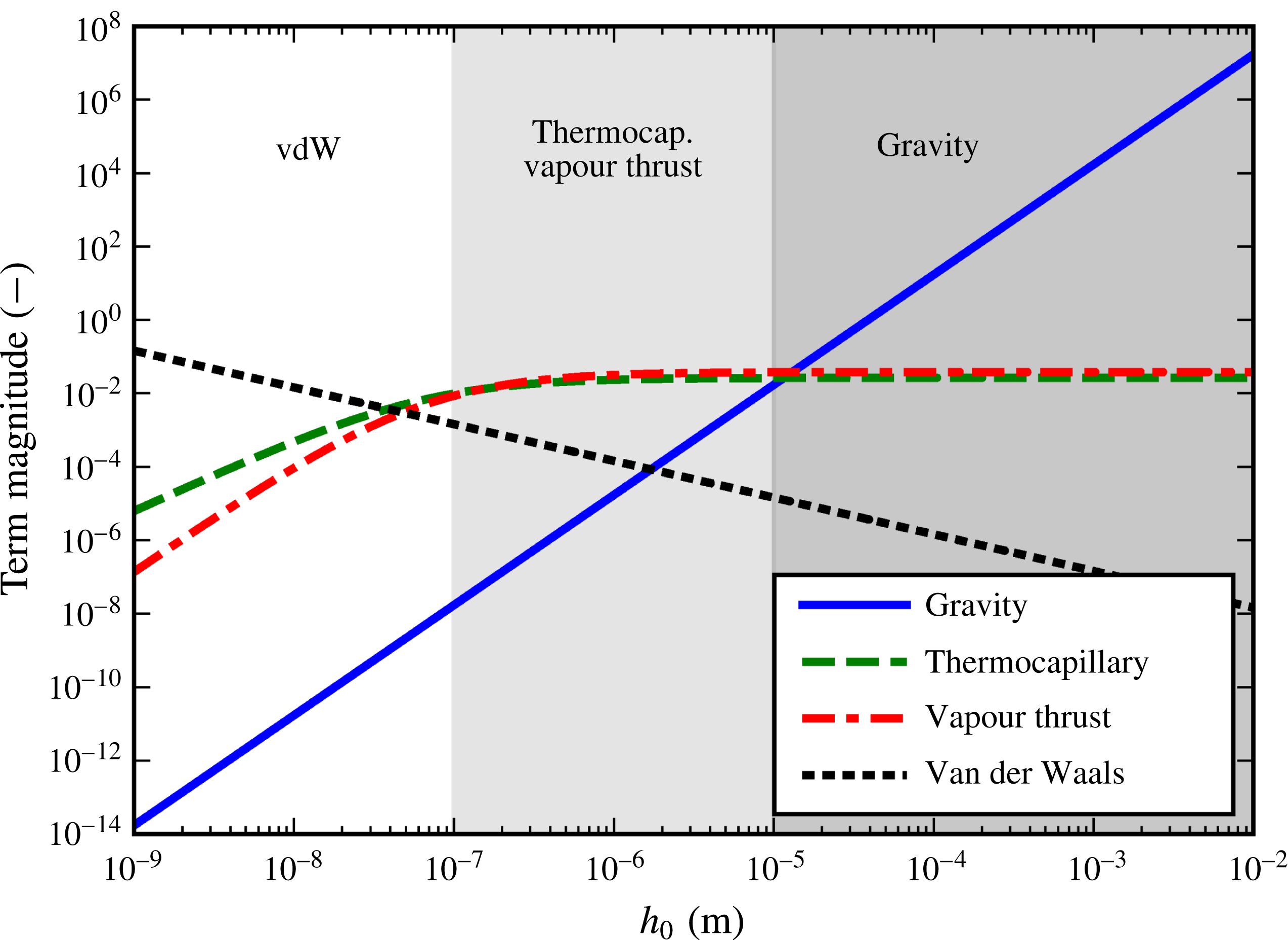
and
 $A>0$
) working against the sole stabilizing vapour thrust term. Their typical dependencies on film-thickness scale are illustrated in figure 4. We note the following features:
(i) For large
$h_{0}$
, the destabilizing influence of gravity will dominate.(ii) For
$h_{0}<100~\text{nm}$
, the destabilizing influence of van der Waals forces will dominate(iii) For intermediate
$h_{0}$
, there is a remarkably even struggle between the destabilizing influence of the thermocapillary effect and the stabilizing influence of the vapour thrust effect.


We see that the vapour film is always predicted to be unstable at very small or very large thickness scales due to the van der Waals and gravity terms, respectively. However, at the intermediate thickness scales the vapour thrust and thermocapillary terms are of similar magnitude but approximately two orders of magnitude larger than the other two. This means that the thermocapillary effect is the only destabilizing effect that is capable of cancelling out the stabilizing vapour thrust in the intermediate thickness range. While the gravity and van der Waals (vdW) terms also work against vapour thrust, their effect is negligible in comparison. In summary, the model suggests the following:
(i) The very small and very large thickness scales are always unstable.
(ii) The intermediate thickness scale can only be unstable if the thermocapillary term overpowers the vapour thrust term.
We may combine these two observations with the following hypothesis:
(i) Hypothesis: observed vapour film collapse (Leidenfrost transition) occurs when there is instability on every thickness scale.
The hypothesis implies that a necessary condition for film boiling collapse is that all three regions indicated in figure 4 are unstable. As stated above, the very small and very large scales are always unstable. This leaves the intermediate scales, which are dominated by the thermocapillary and vapour thrust terms. To be even more specific, film boiling collapse would require instability in the
 $h_{0}>1~\unicode[STIX]{x03BC}\text{m}$
part of the intermediate region. On these scales
 $F_{0}$
approaches unity, as discussed in § 3.3.
Sample values for the terms in (3.4) in the case of water film boiling with
 $\unicode[STIX]{x0394}T=225~\text{K}$
(above the Leidenfrost point), as a function of film-thickness scale
 $h_{0}$
. The different shaded parts have labels indicating the dominant influence(s) in the given region.

In summary, the above hypothesis together with the behaviour of the terms in (3.4) implies that a theoretical predictor for the Leidenfrost point may be found from the balance between the thermocapillary and vapour thrust terms in the
 $F_{0}\rightarrow 1$
limit. Based on this we find the following
 $h_{0}$
-independent criterion for vapour film collapse:
 $$\begin{eqnarray}\displaystyle {\displaystyle \frac{K\tilde{M}}{2E}}>{\displaystyle \frac{\unicode[STIX]{x1D709}E\text{Re}}{6}}. & & \displaystyle\end{eqnarray}$$
The above condition depends on fluid properties as well as the superheat
 $\unicode[STIX]{x0394}T$
. We interpret the
 $\unicode[STIX]{x0394}T$
that satisfies (3.6) as an equality as the Leidenfrost point,
 $\unicode[STIX]{x0394}T_{L}$
. This is the superheat below which film boiling collapse is observed.
Note that the vapour density and conductivity contained in
 $K$
,
 $E$
, and
 $Re$
are supposed to be evaluated at the average film temperature,
 $T_{f}=T_{s}+\unicode[STIX]{x0394}T/2$
, which is initially unknown. We seek an explicit expression for
 $\unicode[STIX]{x0394}T_{L}$
that depends on known saturation properties only. When we insert expressions for the dimensionless constants in (3.6), we get
 $$\begin{eqnarray}\displaystyle {\displaystyle \frac{\unicode[STIX]{x0394}T_{L}}{T_{s}}}=\left({\displaystyle \frac{3\unicode[STIX]{x1D702}}{1+3\unicode[STIX]{x1D702}}}\right){\displaystyle \frac{\sqrt{2\unicode[STIX]{x03C0}R_{s}T_{s}}}{f(\unicode[STIX]{x1D6FC}_{e})k_{v,s}}}\unicode[STIX]{x1D6FE}\left[{\displaystyle \frac{\unicode[STIX]{x1D70C}_{v}}{\unicode[STIX]{x1D70C}_{v,s}}}{\displaystyle \frac{k_{v,s}}{k_{v}}}\right]. & & \displaystyle\end{eqnarray}$$
The left-hand side is a convenient dimensionless quantity which we call the ‘relative Leidenfrost temperature’. We see that (3.7) is an implicit equation for the relative Leidenfrost temperature, since the square bracket also depends on it. For ideal gases at constant pressure we know that
 $\unicode[STIX]{x1D70C}_{v}\sim 1/T$
and
 $k_{v}\sim \sqrt{T}$
, and thus, we may collect all
 $\unicode[STIX]{x0394}T_{L}$
dependence on the left-hand side, giving
 $$\begin{eqnarray}\displaystyle \left(1+{\displaystyle \frac{1}{2}}{\displaystyle \frac{\unicode[STIX]{x0394}T_{L}}{T_{s}}}\right)^{3/2}{\displaystyle \frac{\unicode[STIX]{x0394}T_{L}}{T_{s}}}=\left({\displaystyle \frac{3\unicode[STIX]{x1D702}}{1+3\unicode[STIX]{x1D702}}}\right)\left({\displaystyle \frac{\sqrt{2\unicode[STIX]{x03C0}}}{f(\unicode[STIX]{x1D6FC}_{e})}}\right)\left({\displaystyle \frac{\sqrt{R_{s}T_{s}}}{k_{v,s}}}\right)\unicode[STIX]{x1D6FE}\equiv \unicode[STIX]{x1D6E9}. & & \displaystyle\end{eqnarray}$$
Here the right-hand side, labelled
 $\unicode[STIX]{x1D6E9}$
for short, may be evaluated solely from known saturation properties. Its value is usually considerably less than unity. For small
 $\unicode[STIX]{x0394}T_{L}/T_{s}$
, we may make (3.8) explicit, as
 $$\begin{eqnarray}\displaystyle {\displaystyle \frac{\unicode[STIX]{x0394}T_{L}}{T_{s}}}\approx {\displaystyle \frac{2}{3}}[\sqrt{1+3\unicode[STIX]{x1D6E9}}-1]. & & \displaystyle\end{eqnarray}$$
It turns out that the third parenthesis in
 $\unicode[STIX]{x1D6E9}$
is essentially fluid independent because we generally have that
 $k_{v}\sim \sqrt{R_{s}T}$
, as known from ideal kinetic theory. When we define the (almost constant) variable
 $$\begin{eqnarray}\displaystyle c_{k}={\displaystyle \frac{\sqrt{RT}}{k_{v}}}, & & \displaystyle\end{eqnarray}$$
the expression for
 $\unicode[STIX]{x1D6E9}$
becomes
 $$\begin{eqnarray}\displaystyle \unicode[STIX]{x1D6E9}\approx \left({\displaystyle \frac{3\unicode[STIX]{x1D702}}{1+3\unicode[STIX]{x1D702}}}\right)\left({\displaystyle \frac{c_{k}\sqrt{2\unicode[STIX]{x03C0}}}{f(\unicode[STIX]{x1D6FC}_{e})}}\right)\unicode[STIX]{x1D6FE}. & & \displaystyle\end{eqnarray}$$
If we apply the expression (2.62) for
 $\unicode[STIX]{x1D702}(\unicode[STIX]{x1D6F9})$
, we find that
 $3\unicode[STIX]{x1D702}/(1+3\unicode[STIX]{x1D702})=3/(4+\unicode[STIX]{x1D6F9}^{-1})$
, which gives
 $$\begin{eqnarray}\displaystyle \unicode[STIX]{x1D6E9}\approx \left({\displaystyle \frac{3}{4+\unicode[STIX]{x1D6F9}^{-1}}}\right)\left({\displaystyle \frac{c_{k}\sqrt{2\unicode[STIX]{x03C0}}}{f(\unicode[STIX]{x1D6FC}_{e})}}\right)\unicode[STIX]{x1D6FE}. & & \displaystyle\end{eqnarray}$$
Equation (3.9) with (3.12) constitute the final and relatively simple practical result which may be used to predict the relative Leidenfrost temperature. Given that fluids generally have the same values for
 $\unicode[STIX]{x1D6F9}$
,
 $c_{k}$
and
 $\unicode[STIX]{x1D6FC}_{e}$
, this model predicts that the relative Leidenfrost temperature depends almost solely on
 $\unicode[STIX]{x1D6FE}$
and that this relationship is approximately linear.
4 Experimental validation
We now seek to evaluate the predictive power of the present model by comparing it to experimental observations of
 $\unicode[STIX]{x0394}T_{L}$
. From now on, when we refer to the ‘present model’, we mean (3.9) with (3.12) while using the constant values
 $$\begin{eqnarray}\displaystyle & \displaystyle \overline{c_{k}}=14\,000~\text{K}~\text{m}~\text{N}^{-1}, & \displaystyle\end{eqnarray}$$
 $$\begin{eqnarray}\displaystyle & \displaystyle \overline{\unicode[STIX]{x1D6F9}}=1/30, & \displaystyle\end{eqnarray}$$
which are simply rounded-off averages from the fluids studies here. Constant values for these parameters are used since
 $c_{k}$
and
 $\unicode[STIX]{x1D6F9}$
are very similar for most fluids, compared to the variations in
 $\unicode[STIX]{x1D6FE}$
. Making this choice significantly simplifies the application of the model, and serves to illustrate the point that the model mostly depends on two parameters only:
 $\unicode[STIX]{x1D6FE}$
and
 $\unicode[STIX]{x1D6FC}_{e}\in [0,1]$
. We look up
 $\unicode[STIX]{x1D6FE}$
directly from surface tension data, and use the Schrage form of the kinetic theory evaporation models, equation (2.9).
For each fluid, we look for a single experimentally measured property: the Leidenfrost temperature (
 $T_{L}$
) found at atmospheric pressure. This number is then made dimensionless by considering its relative distance from the saturation temperature
 $T_{s}$
, thus matching the left-hand side of (3.9). The data are shown in table 1.
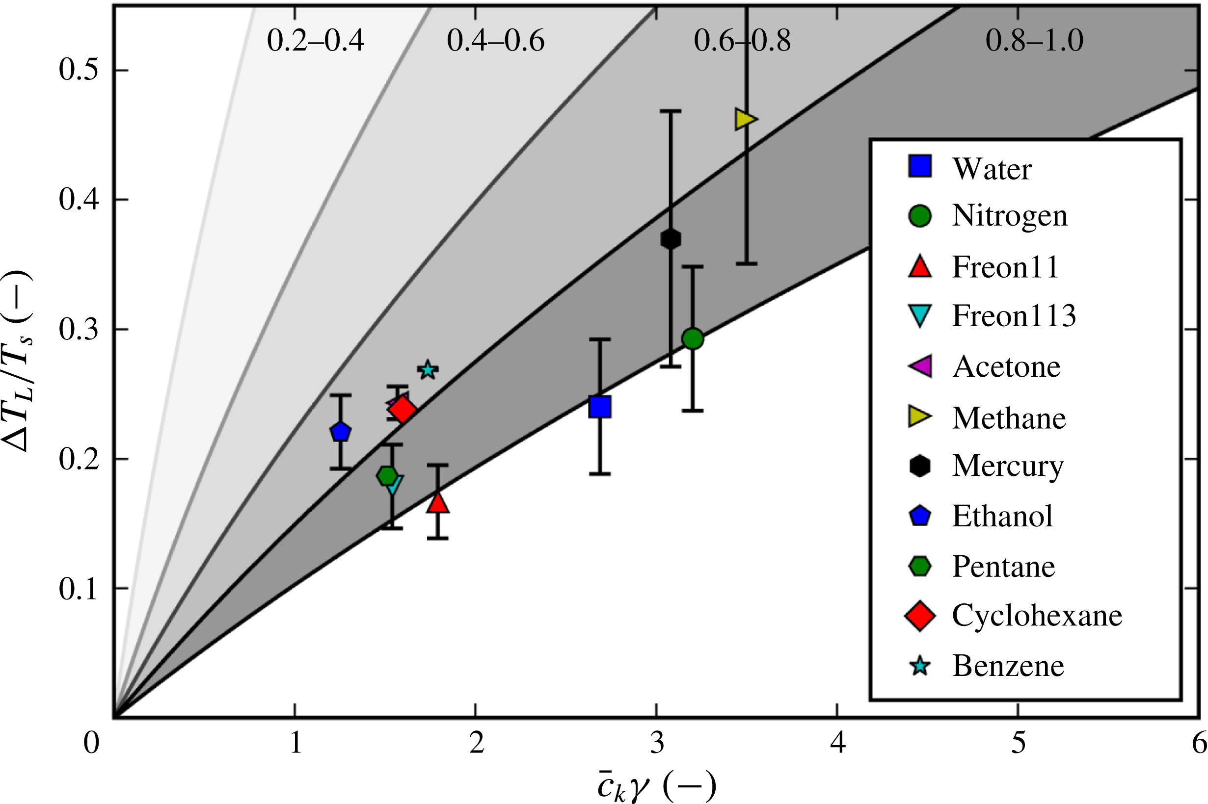
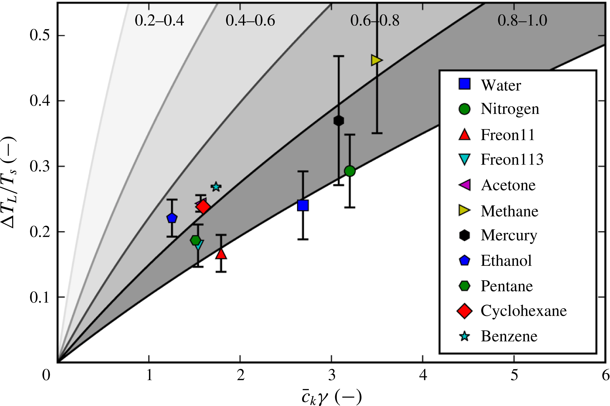
We compare the model with the experimental data in figure 5, where model predictions are shown for the various possible ranges of the evaporation coefficient
 $\unicode[STIX]{x1D6FC}_{e}$
. The figure shows that all data points are at least consistent with the model, in the sense that none of them would imply the impossible value
 $\unicode[STIX]{x1D6FC}_{e}>1$
. The data points all fall within the predictions corresponding to
 $\unicode[STIX]{x1D6FC}_{e}\in (0.7,1.0)$
, but the unknown nature of the evaporation coefficient prevents any accurate confirmation of the dependence on
 $\unicode[STIX]{x1D6FE}$
. The implications of figure 5 are further discussed in § 6.1.
Comparison of the present model with the experimental data shown in table 1. The shaded regions indicate model predictions for different ranges of
 $\unicode[STIX]{x1D6FC}_{e}$
. Error bars indicate the standard deviation of the different data points found in the literature. The lack of an error bar indicates that only a single data point could be found.
5 Comparison with previous Leidenfrost point models
We now seek to evaluate the predictive capabilities of the present model compared to some existing models and correlations for the Leidenfrost point. The models considered here are either based on semi-empirical fluid mechanical considerations or based on the hypothesis that the Leidenfrost point corresponds to the superheat limit. The latter comes in two different versions, depending on how the superheat limit is represented.
5.1 Simplified fluid mechanical models
A semi-empirical model for the Leidenfrost point was developed by Berenson (Reference Berenson1961, equation (40)), who developed a model for the film boiling heat transfer coefficient based on classical Rayleigh–Taylor stability analysis and conservation equations in a simplified geometry. When he combined this with the minimum heat flux model by Zuber (Reference Zuber1959), which also employs simplified fluid mechanical considerations, this resulted in an expression for
 $\unicode[STIX]{x0394}T_{L}$
,
 $$\begin{eqnarray}\displaystyle {\displaystyle \frac{\unicode[STIX]{x0394}T_{L}}{T_{s}}}=0.127{\displaystyle \frac{\unicode[STIX]{x1D70C}_{v}L}{k_{v}T_{s}}}\left({\displaystyle \frac{g\unicode[STIX]{x0394}\unicode[STIX]{x1D70C}}{\unicode[STIX]{x1D70C}_{l}+\unicode[STIX]{x1D70C}_{v}}}\right)^{2/3}\left({\displaystyle \frac{\unicode[STIX]{x1D70E}_{0}}{g\unicode[STIX]{x0394}\unicode[STIX]{x1D70C}}}\right)^{1/2}\left({\displaystyle \frac{\unicode[STIX]{x1D707}_{v}}{g\unicode[STIX]{x0394}\unicode[STIX]{x1D70C}}}\right)^{1/3}. & & \displaystyle\end{eqnarray}$$
Note that (5.1) is semi-empirical. The exponents are theoretically derived, but the pre-factor
 $0.127$
stems from an experimental fit to film boiling data.
5.2 Leidenfrost point from superheat limit
A different class of models is based on the simple hypothesis that the Leidenfrost point corresponds to the liquid superheat limit, also called the homogeneous nucleation temperature. The superheat limit is commonly estimated in two different ways. The first method is by calculating the spinodal temperature from an equation of state. The spinodal is the theoretical absolute maximum superheat temperature, where the vapour nucleation barrier goes to zero. However, homogeneous nucleation will usually proceed spontaneously before the barrier reaches zero, and the temperature where this happens may be approximated by classical nucleation theory (CNT). This is the second method. Both methods are purely theoretical and do not have any fitted empirical parameters. See Aursand et al. (Reference Aursand, Gjennestad, Aursand, Hammer and Wilhelmsen2017) for further discussion on nucleation theory and the spinodal.
Superheat limit from spinodal. Using the spinodal to estimate the Leidenfrost point was first suggested by Spiegler et al. (Reference Spiegler, Hopenfeld, Silberberg, Bumpus and Norman1963). They used the van der Waals equation of state to analytically relate the spinodal (
 $T_{sp}$
) to the critical temperature,
 $T_{sp}=(27/32)T_{c}$
. This implies that the relative Leidenfrost temperature is simply
 $$\begin{eqnarray}\displaystyle {\displaystyle \frac{\unicode[STIX]{x0394}T_{L}}{T_{s}}}={\displaystyle \frac{27}{32}}{\displaystyle \frac{T_{c}}{T_{s}}}-1. & & \displaystyle\end{eqnarray}$$
Superheat limit from nucleation theory. Alternatively, one may use classical nucleation theory to predict the vapour nucleation rate at a given degree of liquid superheating. In combination with high accuracy equations of state, using this to predict the experimental superheat limit has been found to be quite accurate (Aursand et al.
Reference Aursand, Gjennestad, Aursand, Hammer and Wilhelmsen2017). Going one step further and using this to represent the Leidenfrost point is less established but has been suggested by authors such as Yao & Henry (Reference Yao and Henry1978) and Sakurai et al. (Reference Sakurai, Shiotsu and Hata1990). In classical nucleation theory (Aursand et al.
Reference Aursand, Gjennestad, Aursand, Hammer and Wilhelmsen2017) the nucleation rate
 $\unicode[STIX]{x1D6EC}$
(
 $\text{s}-1~\text{m}^{-3}$
) is expressed as an Arrhenius rate law,
 $$\begin{eqnarray}\displaystyle \unicode[STIX]{x1D6EC}=\unicode[STIX]{x1D6EC}_{0}\exp \left(-{\displaystyle \frac{\unicode[STIX]{x0394}G}{k_{B}T}}\right), & & \displaystyle\end{eqnarray}$$
with the activation energy being
 $$\begin{eqnarray}\displaystyle \unicode[STIX]{x0394}G={\displaystyle \frac{16\unicode[STIX]{x03C0}\unicode[STIX]{x1D70E}^{3}(T)}{3(p_{s}(T)-p)^{2}}}, & & \displaystyle\end{eqnarray}$$
and the rate at zero activation barrier being
 $$\begin{eqnarray}\displaystyle \unicode[STIX]{x1D6EC}_{0}={\displaystyle \frac{\unicode[STIX]{x1D70C}_{l}}{m^{3/2}}}\sqrt{{\displaystyle \frac{2\unicode[STIX]{x1D70E}}{\unicode[STIX]{x03C0}}}}. & & \displaystyle\end{eqnarray}$$
Here,
 $m$
is the mass of a single molecule and
 $p_{s}$
is the thermodynamic saturation pressure. The specific expression for
 $\unicode[STIX]{x1D6EC}_{0}$
may vary a little between authors, but this has a negligible effect on the final result for the superheat limit.
The expression in (5.3) simply gives the nucleation rate as a function of fluid properties and temperature. In order to find the superheat limit, one must define a critical nucleation rate
 $\unicode[STIX]{x1D6EC}_{c}<\unicode[STIX]{x1D6EC}_{0}$
, which corresponds to sudden macroscopic phase change. It turns out that due to the rapid growth of the exponential in (5.3), the result is quite insensitive to the specific choice of
 $\unicode[STIX]{x1D6EC}_{c}$
. Here, we use the value of
 $\unicode[STIX]{x1D6EC}_{c}=1\times 10^{12}~\text{s}^{-1}~\text{m}^{-3}$
, as seen in previous works (Bernardin & Mudawar Reference Bernardin and Mudawar1999; Aursand et al.
Reference Aursand, Gjennestad, Aursand, Hammer and Wilhelmsen2017). Thus, in order to predict the superheat limit, we simply have to solve the implicit equation
 $$\begin{eqnarray}\displaystyle \unicode[STIX]{x1D6EC}(T)=\unicode[STIX]{x1D6EC}_{c} & & \displaystyle\end{eqnarray}$$
for
 $T$
. Note that it is absolutely essential to include the temperature dependence of
 $\unicode[STIX]{x1D70E}$
in (5.4), as it is one of the major sources of temperature dependence in
 $\unicode[STIX]{x0394}G$
. In order to obtain a model of comparable simplicity and avoid having to iteratively solve for the saturation line using an equation of state, we use the Clausius–Clapeyron relation to estimate the saturation pressure as
 $$\begin{eqnarray}\displaystyle p_{s}(T)=p\exp \left[{\displaystyle \frac{L}{R_{s}}}\left({\displaystyle \frac{1}{T_{s}(p)}}-{\displaystyle \frac{1}{T}}\right)\right]. & & \displaystyle\end{eqnarray}$$
5.3 Performance comparison
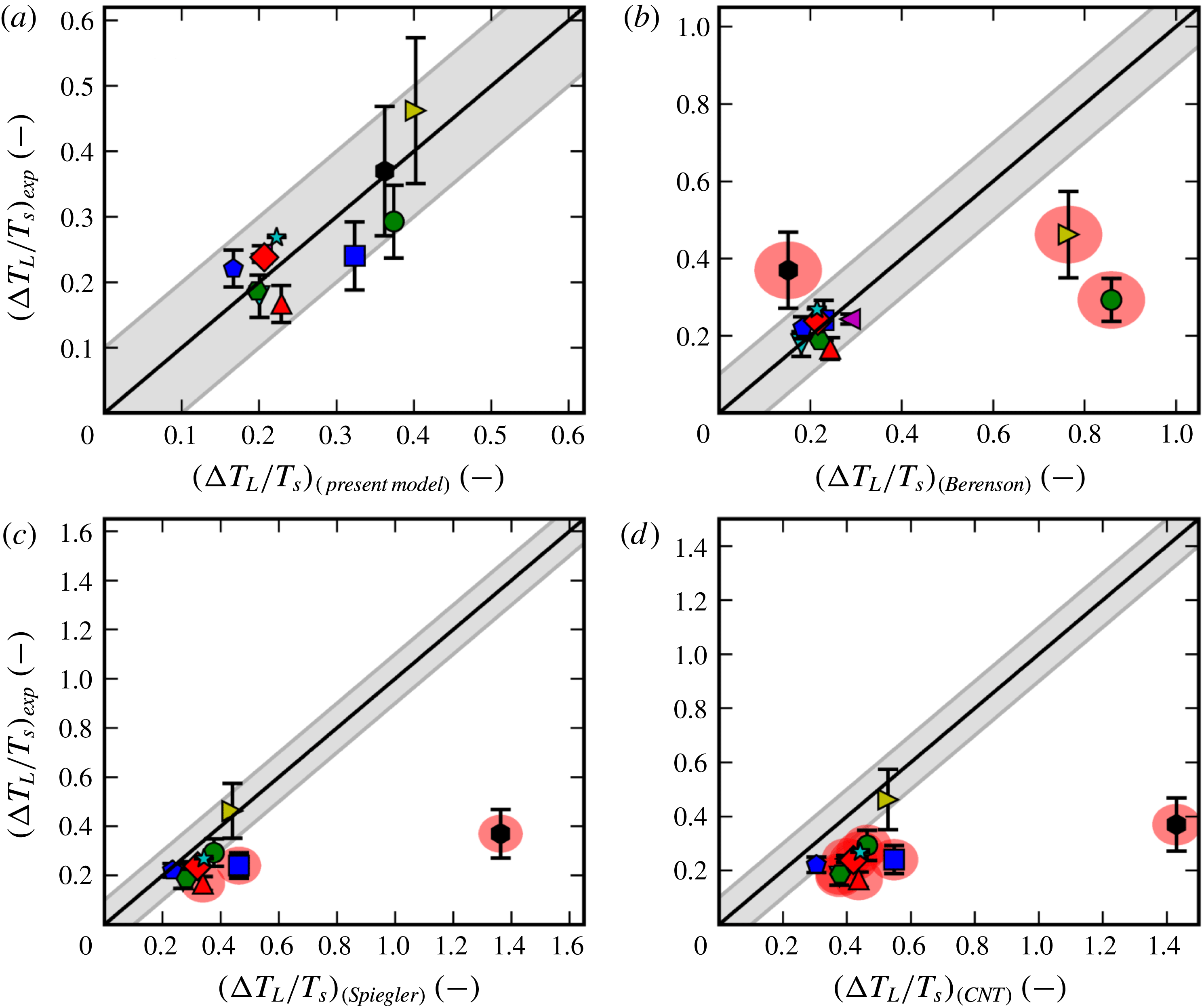
We now seek to compare the predictive performance of the present model with the three alternative models presented in § 5.1 (Berenson model) and § 5.2 (Spiegler model and CNT model). Since
 $\unicode[STIX]{x1D6FC}_{e}$
can generally be anywhere in the range of
 $(0,1)$
, well-defined prediction by the present model requires the choice of a specific value. Here, we choose
 $\unicode[STIX]{x1D6FC}_{e}=0.85$
, which is the centre point of the expected range identified in § 2.2. The fluid properties necessary to evaluate the other models were mainly found from the NIST database (Linstrom & Mallard Reference Linstrom and Mallard2017; Dean Reference Dean1998). Missing mercury properties were found in Skapski (Reference Skapski1948), Epstein & Powers (Reference Epstein and Powers1953), Vinogradov (Reference Vinogradov1981) and Huber, Laesecke & Friend (Reference Huber, Laesecke and Friend2006).
The evaluation of predictive performance is shown in figure 6, where we see that only the present model can accurately predict the relative Leidenfrost point within an error of
 $10\,\%$
for every fluid. This is further discussed in § 6.2.
Comparison of model predictions with experimental data for the relative Leidenfrost point for (a) the present model (with
 $\unicode[STIX]{x1D6FC}_{e}=0.85$
), (b) the Berenson model (5.1), (c) the Spiegler model (5.2) and (d) the CNT model (5.6). See figure 5 for data point legend. Grey bands show the range of a
 $\pm 10\,\%$
error in prediction of
 $T_{L}$
, relative to
 $T_{s}$
. Data points that fall outside this band are marked with red circles.
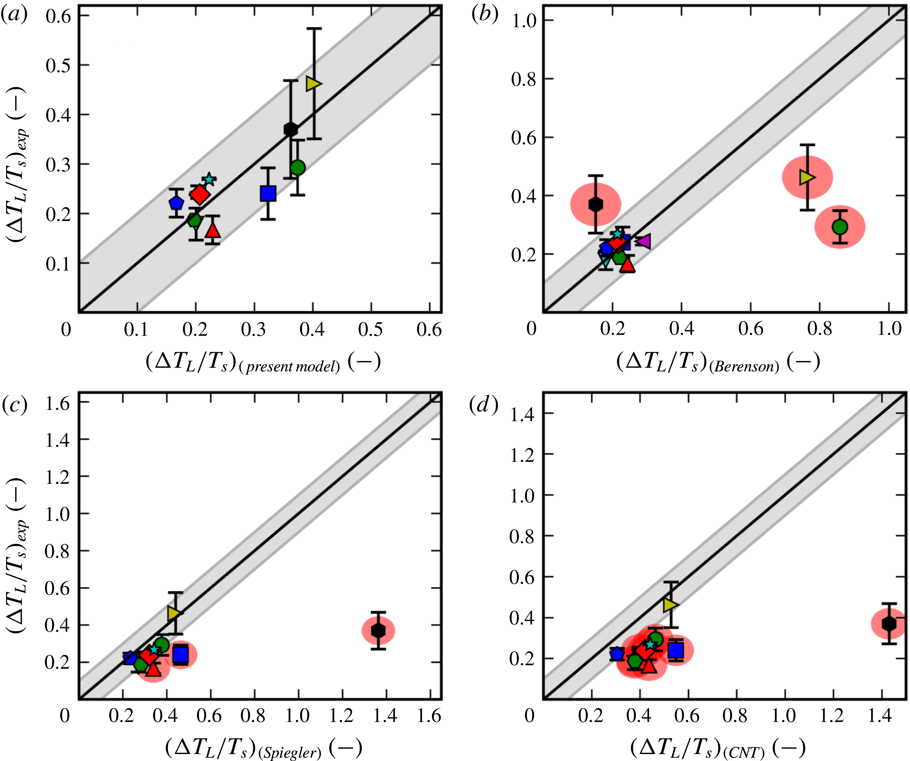
6 Discussion
6.1 Model validity and predictive power
The present model for the Leidenfrost point depends on the somewhat unknown evaporation coefficient
 $\unicode[STIX]{x1D6FC}_{e}$
, which is generally unknown but always lies within the range
 $(0,1)$
. The model predicts that
 $\unicode[STIX]{x0394}T_{L}\rightarrow \infty$
when
 $\unicode[STIX]{x1D6FC}_{e}\rightarrow 0$
, and thus, generally the model merely provides a lower bound on
 $\unicode[STIX]{x0394}T_{L}$
given by the
 $\unicode[STIX]{x1D6FC}_{e}=1$
result. In terms of figure 5, this means that any data point above the bottom line (
 $\unicode[STIX]{x1D6FC}_{e}=1$
) is consistent with the model. As discussed in § 2.2, molecular dynamics simulations indicate that
 $\unicode[STIX]{x1D6FC}_{e}$
should be within the range 0.7–1.0. This is consistent with every data point seen in figure 5. Note that data points falling above the bottom line in figure 5 may also be explained by imperfect wall temperature control (
 $Bi_{w}^{-1}>0$
). On the other hand, if any data points were to fall significantly below the bottom line, that would count as evidence against the model. In this sense, the model is still falsifiable.
Qualitatively, the present model predicts that to a good approximation
 $\unicode[STIX]{x0394}T_{L}/T_{s}$
only depends on
 $\unicode[STIX]{x1D6FE}$
and
 $\unicode[STIX]{x1D6FC}_{e}$
. Whereas all the data found are quantitatively consistent with the model, the
 $\unicode[STIX]{x1D6FE}$
dependence is not satisfactorily tested since all the fluids with available Leidenfrost data have
 $\unicode[STIX]{x1D6FE}$
-values within the same order of magnitude. Given this limited range of
 $\unicode[STIX]{x1D6FE}$
, we see in figure 5 that any good confirmation of the
 $\unicode[STIX]{x1D6FE}$
dependence is muddled by uncertainty in
 $\unicode[STIX]{x1D6FC}_{e}$
. However, just as important as the prediction of
 $\unicode[STIX]{x1D6FE}$
-dependence is the predicted independence on very variable fluid properties such as
 $T_{s}$
,
 $\unicode[STIX]{x1D70E}_{0}$
or
 $L$
. While the fluids studied here have very variable values of these three parameters (even different orders of magnitude), they have values of
 $\unicode[STIX]{x0394}T_{L}/T_{s}$
within the same order of magnitude. This is correctly predicted by the present model.
Despite the fact that every data point is consistent with the model, the relatively uncertain nature of the evaporation coefficient may pose a problem for the predictive power of the model. Without any additional information on
 $\unicode[STIX]{x1D6FC}_{e}$
for a specific fluid, we have little choice but to assume a value. Thankfully, as we saw in figure 6(a), choosing the centre of the expected interval (
 $\unicode[STIX]{x1D6FC}_{e}=0.85$
) yields a correct prediction for every data point within 10 % error. Additionally, the prediction of a lower bound on
 $\unicode[STIX]{x0394}T_{L}$
appears to be without flaw, as seen in figure 5.
Finally, an interesting observation can be made by looking at the effect of uncertainty in
 $\unicode[STIX]{x1D6FC}_{e}$
on the predicted Leidenfrost temperature. The review in § 2.2 implies that the uncertainty in
 $\unicode[STIX]{x1D6FC}_{e}$
is of the order of 10 %. Around the presumed average point
 $\unicode[STIX]{x1D6FC}_{e}=0.85$
, a change of
 $\pm 10\,\%$
in
 $\unicode[STIX]{x1D6FC}_{e}$
implies a change of approximately
 $\mp 20\,\%$
in the quantity
 $\unicode[STIX]{x0394}T_{L}/T_{s}$
, as we may also see from the width of the shaded bands in figure 5. As an approximate general rule, this means that the uncertainty in absolute
 $T_{L}$
(K) due to
 $\unicode[STIX]{x1D6FC}_{e}$
is about 5 % of the fluid’s saturation temperature. For the fluids where we have a sufficient number of data points to know the underlying variance with decent confidence, this 5 % rule corresponds remarkably well with the experimental standard deviation numbers in table 1. For water the model predicts an uncertainty of 18.7 K while the data have a standard deviation of 19.4 K. For nitrogen the model predicts an uncertainty of 3.87 K while the data have a standard deviation of 4.31 K. This may suggest that the reason for the relatively large variability in
 $T_{L}$
measurements is that
 $\unicode[STIX]{x1D6FC}_{e}$
varies between experiments, not because of any flaws in the Leidenfrost measurements. The fact that the present model can seemingly predict this variation gives it some additional credibility.
Overall, there are compelling pieces of evidence for the hypothesis that the thermocapillary instability is the governing effect behind film boiling collapse. However, there is insufficient available data to be certain.
6.2 Benefits over existing models/correlations
As shown in § 5 and especially in figure 6, the quantitative predictive power for the Leidenfrost point seems to be stronger in the present model compared to the three alternative models considered here. While the alternative models work reasonably well for conventional fluids, they are vastly erroneous for some of the more unusual fluids. Specifically, the Berenson model underpredicts the value for mercury and vastly overpredicts the value for the cryogens nitrogen and methane. The superheat limit based models moderately overpredict the conventional fluids and vastly overpredict the value for mercury. These problems are likely due to these fluids having unconventional values for saturation temperature and/or surface tension. Among the previous models, the semi-empirical Berenson model appears to quantitatively perform the best for conventional fluids, as seen in figure 6(b). However, the data do not appear to correlate in the suggested way. The model simply cuts through the group of data points from conventional fluids, while completely missing the fluids such as mercury and the cryogens, which were likely not part of the original parameter fitting.
Overall, we may claim that the present model for the Leidenfrost point has the following benefits:
(i) Simplicity: there is no need to know a large variety of fluid properties in order to make a prediction. Only a measured value for
$\unicode[STIX]{x1D6FE}$
and an assumption regarding
$\unicode[STIX]{x1D6FC}_{e}$
is needed.(ii) Accuracy: given only the value of
$\unicode[STIX]{x1D6FE}$
, the present model is able to predict
$\unicode[STIX]{x0394}T_{L}$
within an error of 10 % for every fluid considered here, including the cryogen and the liquid metal.(iii) Insight: the model is purely theoretical, i.e. it involves no empirical parameters fitted to film boiling experiments. Such models are not only expected to have greater predictive capabilities, but are also more likely to provide insight into the physical mechanisms behind film boiling collapse. Specifically, the present model suggests that the mechanism of collapse is that the thermocapillary instability overpowers vapour thrust stabilization. To our knowledge, this has not been suggested before.


6.3 Prediction in the absence of thermocapillary effect
Note that this model’s prediction of the Leidenfrost point is completely dependent on two complicating effects: non-equilibrium evaporation model and non-trivial liquid shear rate. Making either the approximation of quasi-equilibrium or zero liquid velocity would eliminate the thermocapillary effect from the model.
We may ask what the model would predict for the relative Leidenfrost temperature if the thermocapillary effect is absent, such as in the quasi-equilibrium limit (
 $K\rightarrow 0$
). First of all, as discussed and made explicit in (3.4), this will completely remove the thermocapillary effect. If we go back to figure 4 and make the same kind of arguments as before, we see that film boiling collapse would necessitate that the gravity term is stronger than the vapour thrust in the intermediate region. This requirement leads to the criterion
 $$\begin{eqnarray}\displaystyle {\displaystyle \frac{G}{12E}}>{\displaystyle \frac{E\text{Re}}{6(1+Bi_{w}^{-1})^{3}}}, & & \displaystyle\end{eqnarray}$$
which leads to the following prediction for the relative Leidenfrost point:
 $$\begin{eqnarray}\displaystyle {\displaystyle \frac{\unicode[STIX]{x0394}T_{L}}{T_{s}}}=\sqrt{{\displaystyle \frac{\unicode[STIX]{x1D70C}_{v}\unicode[STIX]{x0394}\unicode[STIX]{x1D70C}g}{2}}}{\displaystyle \frac{L}{k_{v}T_{s}}}[(1+Bi_{w}^{-1})h_{0}]^{3/2}. & & \displaystyle\end{eqnarray}$$
Qualitatively, equation (6.2) predicts that the relative Leidenfrost temperature is dependent on both
 $T_{s}$
and
 $L$
. As mentioned previously, this is not supported by the data. Note that (6.2) is dependent on the film-thickness scale
 $h_{0}$
. If we make the assumption that we only need gravity to overpower vapour thrust down to the
 $1~\unicode[STIX]{x03BC}\text{m}$
scale before van der Waals forces take over, we still find that
 $\unicode[STIX]{x0394}T_{L}/T_{s}\approx 0.02$
for
 $\text{H}_{2}\text{O}$
and
 $\unicode[STIX]{x0394}T_{L}/T_{s}\approx 0.05$
for
 $\text{N}_{2}$
, both of which are approximately an order of magnitude below the experimental values in figure 5. Thus, the quasi-equilibrium limit of this model appears useless for predicting vapour film collapse.
6.4 Modifying the Leidenfrost point
It has been reported by authors such as Qiao & Chandra (Reference Qiao and Chandra1997) that adding surfactant (reducing
 $\unicode[STIX]{x1D70E}_{0}$
) reduces the Leidenfrost temperature, i.e. it makes film boiling more stable. Without considering the thermocapillary instability, this seems counter-intuitive, since reducing surface tension would be expected to have a destabilizing effect, if any.
The present model can explain this qualitative effect. Since surface tension must reach zero at the fluid’s critical point, if we can assume that
 $\unicode[STIX]{x1D6FE}$
is close to temperature independent it must be given by
 $$\begin{eqnarray}\displaystyle \unicode[STIX]{x1D6FE}\approx {\displaystyle \frac{\unicode[STIX]{x1D70E}_{0}}{T_{c}-T_{s}}}, & & \displaystyle\end{eqnarray}$$
where
 $T_{c}$
is the critical temperature of the fluid and
 $\unicode[STIX]{x1D70E}_{0}$
is the surface tension at the saturation temperature. Note that (6.3) does not imply that fluids with large surface tension necessarily will have a large
 $\unicode[STIX]{x1D6FE}$
. Water and especially mercury have large surface tensions but still quite ordinary
 $\unicode[STIX]{x1D6FE}$
values. Given this the present model provides a new explanation for this observation: reducing
 $\unicode[STIX]{x1D70E}_{0}$
for a given fluid will reduce
 $\unicode[STIX]{x1D6FE}$
through (6.3) and thus weaken the thermocapillary instability relative to the vapour thrust.
A commonly suggested method of modifying the Leidenfrost point is through the solid surface topography, such as addition of micro- or nanostructures (Auliano et al. Reference Auliano, Fernandino, Zhang and Dorao2017). This cannot be predicted by this model in its present form, as a flat and smooth solid surface has been assumed from the beginning.
7 Conclusions
In summary:
(i) We presented governing equations for vapour flow in film boiling. Of particular importance and novelty was the use of a non-equilibrium evaporation model based on kinetic theory, which allowed for the inclusion of thermocapillary effects along the evaporating liquid–vapour interface.
(ii) We used the long-wave approximation and simplified liquid dynamics to derive a single highly nonlinear scalar PDE for the film thickness function: (2.66).
(iii) We applied linear stability analysis to the above mentioned PDE and identified four terms which govern the long-wave stability of a uniform vapour film: (3.4). Analysis of their dependence on film-thickness scale revealed that the question of stability at the intermediate (micrometre) scale is primarily a struggle between destabilizing thermocapillary effects and stabilizing vapour thrust. The scales above and below are always unstable.
(iv) We posed the hypothesis that film boiling collapse occurs when the film is unstable for any film-thickness scale. According to the present stability analysis, this would necessitate that thermocapillary instabilities overpower vapour thrust.
(v) Based on the above hypothesis we derived a relatively simple model for the Leidenfrost temperature, equations (3.9) with (3.12), which mainly depends on
$\unicode[STIX]{x1D6FE}$
, the temperature dependence of surface tension.(vi) We gathered experimental data for 11 different fluids and showed how the model is consistent with the average Leidenfrost temperature for every one of them given that the evaporation coefficient is in the range 0.7–1.0. As mentioned in § 2.2, this range for
$\unicode[STIX]{x1D6FC}_{e}$
is consistent with recent evaporation/condensation studies using molecular dynamics simulations.(vii) We showed how the assumption of evaporation coefficient equal to 0.85 can successfully predict the Leidenfrost point for each of the fluids within
$10\,\%$
error, a feat that commonly cited models/correlations could not perform.


The present model is a completely theoretical prediction and involves no empirical parameters fitted to film boiling experiments. This allows us to draw conclusions regarding the underlying phenomena. We have found compelling but preliminary evidence to support the following statements:
(i) The governing mechanism behind film boiling collapse (Leidenfrost transition) may be the thermocapillary instability at the liquid–vapour interface. The thermocapillary instability at an evaporating interface is closely connected to non-equilibrium evaporation effects.
(ii) The relative Leidenfrost point,
$\unicode[STIX]{x0394}T_{L}/T_{s}$
, depends almost linearly on
$\unicode[STIX]{x1D6FE}$
, the temperature dependence of surface tension.(iii) The relative Leidenfrost point also depends on the evaporation coefficient
$\unicode[STIX]{x1D6FC}_{e}$
from kinetic theory. Its value is generally unknown but the range 0.7–1.0 gives consistency with all the data. The maximum value of 1.0 gives a reliable lower bound, and the central value 0.85 gives overall good prediction.


Additional research is needed to further validate or disprove these conclusions. Efforts should be made to identify fluids with uncommon (high or low) values of
 $\unicode[STIX]{x1D6FE}$
and then measure their Leidenfrost point. While any data points in the shaded regions of figure 5 is consistent with the model, any new points below would count as evidence against it. Finally, it would be very helpful to resolve some of the uncertainty regarding the evaporation coefficient, as it would sharpen the prediction of the model and put it to a stronger test. This could be resolved with a combination of theory and experiments.
Acknowledgements
E.A. was supported by the Research Council of Norway [244076/O80] and The Gas Technology Centre (NTNU–SINTEF) through the funding programme MAROFF. His research visit at Northwestern University was supported by the US-Norway Fulbright Foundation. Additional thanks to Bernhard Müller, Svend Tollak Munkejord and Morten Hammer for discussions and feedback.
Appendix A. Liquid velocity profile and the value of
$\unicode[STIX]{x1D702}$

In § 2.7.4 the issue of the unknown liquid velocity profile was handled by interpolating the interface velocity between the two calculable theoretical extremes: the case of zero interface velocity, and the case of zero liquid shear. The specific point on the interpolation was set by the unknown parameter
 $\unicode[STIX]{x1D702}\in [0,1]$
.
In this section we explore what a specific assumption regarding the liquid velocity profile implies for the value of
 $\unicode[STIX]{x1D702}$
. We follow the method proposed in Aursand (Reference Aursand2018), and assume a liquid velocity profile of the form
 $$\begin{eqnarray}\displaystyle U_{l}\sim {\displaystyle \frac{1}{Z}}. & & \displaystyle\end{eqnarray}$$
While (A 1) is arguably quite ad hoc, it has the desirable property of monotonically and smoothly decreasing to zero value (and zero derivatives) as
 $Z\rightarrow \infty$
. If we now combine the velocity profiles (2.52) and (A 1) with the boundary conditions (2.29) and (2.32), we may solve explicitly for the vapour velocity profile,
 $$\begin{eqnarray}\displaystyle U & \displaystyle ={\displaystyle \frac{1}{2}}\bar{P}_{X}\left(Z^{2}-{\displaystyle \frac{2+\unicode[STIX]{x1D6F9}^{-1}}{1+\unicode[STIX]{x1D6F9}^{-1}}}HZ\right)-{\displaystyle \frac{1}{1+\unicode[STIX]{x1D6F9}^{-1}}}\unicode[STIX]{x1D716}M(\unicode[STIX]{x1D703}_{i})_{X}Z, & \displaystyle\end{eqnarray}$$
and the interface velocity,
 $$\begin{eqnarray}\displaystyle U_{i}={\displaystyle \frac{1}{1+\unicode[STIX]{x1D6F9}^{-1}}}\left(-{\displaystyle \frac{1}{2}}H^{2}\bar{P}_{X}-\unicode[STIX]{x1D716}MH(\unicode[STIX]{x1D703}_{i})_{X}\right). & & \displaystyle\end{eqnarray}$$
If we compare (A 3) with its generic version (2.60), we see that
 $$\begin{eqnarray}\displaystyle \unicode[STIX]{x1D702}={\displaystyle \frac{1}{1+\unicode[STIX]{x1D6F9}^{-1}}}=\unicode[STIX]{x1D6F9}+\mathit{O}(\unicode[STIX]{x1D6F9}^{2}). & & \displaystyle\end{eqnarray}$$
Appendix B. Liquid heat transfer
In § 2.7.2, the shorthand
 $C=1+C^{\prime }$
was introduced to express the solution to the energy equation, with the small deviation from unity being
 $$\begin{eqnarray}\displaystyle C^{\prime }\equiv Bi_{l}K={\displaystyle \frac{\tilde{K}\unicode[STIX]{x1D6FC}_{l}}{L}}. & & \displaystyle\end{eqnarray}$$
Note that while
 $Bi_{l}$
and
 $K$
individually are dependent on
 $h_{0}$
,
 $C$
is not. Since
 $Bi_{l}$
does not appear outside of
 $C$
in the model, all influence of liquid heat transfer in the dimensionless equations turns out to be independent of film-thickness scale.
The present model assumes that the liquid bulk is held at the saturation temperature. To be more precise, one could state that the temperature is regulated to
 $T_{s}$
a constant distance
 $z=\unicode[STIX]{x0394}z_{l}\gg h_{0}$
from the solid wall. The heat transfer coefficient in the liquid,
 $\unicode[STIX]{x1D6FC}_{l}$
, may then be expressed as a conductive contribution multiplied by a Nusselt number (
 $Nu$
) to account for possible convective enhancement,
 $$\begin{eqnarray}\displaystyle \unicode[STIX]{x1D6FC}_{l}=Nu{\displaystyle \frac{k_{l}}{\unicode[STIX]{x0394}z}}. & & \displaystyle\end{eqnarray}$$
If we use water as an example,
 $$\begin{eqnarray}\displaystyle & \displaystyle \tilde{K}\approx 0.14~\text{K}~\text{m}^{2}~\text{s}~\text{kg}^{-1}, & \displaystyle\end{eqnarray}$$
 $$\begin{eqnarray}\displaystyle & \displaystyle L\approx 2\times 10^{6}~\text{J}~\text{kg}^{-1}, & \displaystyle\end{eqnarray}$$
 $$\begin{eqnarray}\displaystyle & \displaystyle k_{l}\approx 0.7~\text{W}~\text{m}^{-1}~\text{K}^{-1}, & \displaystyle\end{eqnarray}$$
and assume that the liquid temperature control happens on the scale of
 $\unicode[STIX]{x0394}z\sim 1~\text{cm}$
, the small parameter becomes
 $$\begin{eqnarray}\displaystyle C^{\prime }=Nu{\displaystyle \frac{\tilde{K}k_{l}}{L\unicode[STIX]{x0394}z}}\approx Nu\times 10^{-6}. & & \displaystyle\end{eqnarray}$$
Due to the small velocities and temperature differences in the liquid, we may likely assume that the convective enhancement is laminar and weak, i.e.
 $Nu\sim \mathit{O}(1)$
. Thus, we get
 $C^{\prime }\lll 1$
, and we may assume
 $$\begin{eqnarray}\displaystyle C\approx 1 & & \displaystyle\end{eqnarray}$$
for the remaining analysis.
This means that the energy transferred from the interface to the liquid bulk is negligible compared to the energy spent on evaporation, no matter the film thickness
 $h_{0}$
. This can be explained by the fact that the interface temperature is only slightly different from the saturation temperature (
 $\unicode[STIX]{x1D703}_{i}\sim K$
). While the interface temperature increases if the film becomes thinner, so does the evaporation rate, so the former remains negligible.
Note that if one considers subcooled film boiling instead, i.e. a bulk liquid temperature considerably below saturation, the liquid heat transfer is no longer negligible.