1. Introduction
Multi-robot systems (MRSs) allow simpler, cheaper, modular robotic units to be reorganized into a group based on the task at hand. It can be as effective as a task-specific, larger, monolithic robot, which may be more expensive and has to be rebuilt according to the task. Inspired by nature, MRS has evolved into a variety of forms, such as multiple mobile robots [Reference Morsy, Al-Otaibi, Salamah and Ahmad1], multiple manipulators [Reference Kim and Park2], and multiple drones [Reference Zhan, Chen, Chen and Zhang3], and has been applied in various scenarios like construction [Reference Petersen, Napp, Stuart-Smith, Rus and Kovac4] and transportation [Reference Raptis and Sullivan5].
Compared with a single robot, the fundamental challenge of the MRS lies in the cooperation among robots. Cooperation may happen in several aspects, such as knowledge sharing and physical manipulation. In this paper, we focus on the motion planning of the MRS when they fulfill some cooperative transportation tasks.
As a combination of the mobile robot and the manipulator, mobile manipulator (MM) inherits the mobility from the mobile robot and the dexterity from the manipulator. Compared with the two subsystems, MM is redundant. This implies that the same task at the end effector can be executed in different ways in the configuration space, which gives the possibility of optimizing the joint configuration, such as avoiding obstacles. When the object and the robots are rigidly connected, closed-chain will form and the motion of the whole system will be restricted to a lower-dimensional manifold, the connectivity of which will be further affected by various obstacles in the environment [Reference Kingston, Moll and Kavraki6]. Therefore, closed-chain, redundancy, and obstacle-avoidance are coupled and make the motion planning of multiple MMs complicated [Reference Ebel, Rosenfelder and Eberhard7].
1.1. Related works
Localization and navigation of mobile robots serve as the foundation for MRS. In ref. [Reference Chen, Liang, Yuan, Cao and Xie9], a novel concept termed relative localizability was introduced to characterize whether a multi-robot system can achieve mutual localization. The results demonstrated that relative localization in such systems can be accomplished in a purely algebraic and distributed manner. Meanwhile, ref. [Reference Chen, Shorinwa, Bruno, Swann, Yu, Zeng, Nagami, Dames and Schwager10] proposed a real-time navigation pipeline for robots operating in Gaussian Splatting scenes. The pipeline comprises two modules – Splat-Plan and Splat-Loc – which work collaboratively to enable recursive re-planning of smooth and collision-free trajectories toward target locations. Recently, visual-language models have been leveraged to enhance robot navigation in cluttered environments. For instance, ref. [Reference Qi, Zhang, Yu, Wang and Zhao11] introduced an end-to-end framework that utilizes large vision-language models to directly map egocentric video streams into continuous navigation actions. By employing supervised and reinforcement fine-tuning strategies, the model achieved strong performance on the VLN-CE benchmark.
Redundancy in the MM can be resolved within the null space of the Jacobian, which corresponds to subsets of the joint space where the robot can move without affecting the primary task. In ref. [Reference Zhang, Zhang, Xiong, Sheng and Zhu13], the motion of the end effector and that of the mobile robot were treated as the primary and additional tasks, respectively. Experimental results demonstrated that the manipulator could successfully grasp an object while the mobile robot was in motion. In ref. [Reference Fabregat-Jaén, Peidró, Colombo, Rocco and Reinoso12], self-motion manifolds (SMMs) are introduced to model such redundancy. Given a task trajectory, a graph composed of SMMs is constructed and iteratively searched to identify a feasible path. The core challenge in redundancy resolution lies in satisfying additional constraints – such as manipulator dexterity, mobile robot obstacle avoidance, and system formation – while adhering to the prescribed end-effector motion. For instance, our previous work [Reference Zhang, Sheng, Hu, Sheng, Xiong and Zhu24] took into account the dexterity of the MM, obstacle avoidance for the mobile robot, and the overall system formation, thereby enabling intuitive human–robot cooperative transportation.
Closed-chain constrained manifold has its dimension lower than that of the configuration space; hence, uniform sampling in the configuration space has zero probability of generating a valid state that satisfies this constraint [Reference Kingston, Moll and Kavraki6]. One solution to this problem is introducing an allowable tolerance [Reference Bonilla, Pallottino and Bicchi15]. Therefore, the volume of the satisfying subset grows, and various sampling-based motion planners for the unconstrained problem can be adopted. However, much of the complexity of handling the constraint transfers from the higher-level motion planner to the lower-level motion controller. In the case that multiple robots are rigidly connected, motion deviation caused by constraint relaxation may damage the robots and the transported object.
Another popular approach to resolve the closed-chain constraint is Projection (PJ). Several algorithms were developed based on it, such as RGD [Reference Yakey, LaValle and Kavraki16] and CBiRRT [Reference Berenson, Srinivasa and Kuffner17]. However, the constrained Jacobian is not guaranteed to be invertible all the time, and this approach relies heavily on the gradient descent operation, which is time-consuming for the high-dimensional MRS. For example, ref. [Reference Zhang, Yan, Lam and Vijayakumar18] realized the motion planning of three MMs in the simulated environment, but the mean planning time is over one minute. To improve the computational efficiency, Atlas (AT) [Reference Jaillet and Porta19], which uses piece-wise tangent spaces to locally approximate the constrained manifold, and Tangent Bundle (TB) [Reference Kim, Um, Suh and Park20], which is similar to AT but with lazy state checking, were proposed. However, to get the tangent space, the kernel of the constrained Jacobian has to be computed, which requires complex matrix decomposition. Therefore, the computational efficiency of this framework will be reduced.
In addition, to simplify the complex motion planning problem, several works try to solve the 3D transportation tasks into 2D formation control tasks [Reference Oh, Park and Ahn21]. For example, ref. [Reference Tang, Zhang, Yu and Zhang22] defined a 2D virtual structure on the ground named system outlined rectangle (SOR), and the leader–follower approach was applied to plan the motion of the system, where the leader adjusted the width of the SOR according to the environment. Similarly, the convex region was defined in ref. [Reference Alonso-Mora, Baker and Rus23], and then formation control was transformed into an optimization problem with respect to (w.r.t.) the convex region. However, the obstacle-avoidance strategies in [Reference Tang, Zhang, Yu and Zhang22, Reference Alonso-Mora, Baker and Rus23, Reference Jiao, Cao, Gu, Nahavandi, Yang and Tan25] are conservative. As long as the virtual structure (e.g., SOR or convex region) intersects with obstacles, the system is considered in collision. Therefore, bypassing becomes the only way to avoid obstacles, no matter how small they are (see Figure 1).
Robot path planned by algorithms based on the virtual structure [Reference Tang, Zhang, Yu and Zhang22, Reference Alonso-Mora, Baker and Rus23, Reference Jiao, Cao, Gu, Nahavandi, Yang and Tan25]. The dotted lines represent the virtual polygon that encircles the robots and the object. Compared with the path in Figure 5(b), the proposed motion planner is able to find a shorter path that crosses obstacles, while refs. [Reference Tang, Zhang, Yu and Zhang22, Reference Alonso-Mora, Baker and Rus23, Reference Jiao, Cao, Gu, Nahavandi, Yang and Tan25] only find a longer path that bypasses obstacles.

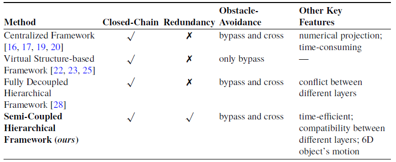
The above works (projection-based [Reference Yakey, LaValle and Kavraki16, Reference Berenson, Srinivasa and Kuffner17, Reference Jaillet and Porta19, Reference Kim, Um, Suh and Park20] and virtual structure-based [Reference Tang, Zhang, Yu and Zhang22, Reference Alonso-Mora, Baker and Rus23, Reference Jiao, Cao, Gu, Nahavandi, Yang and Tan25] algorithms) plan the motion of the object and the robots at the same time, which can be seen as fully centralized methods. As the number of robots increases or the environment becomes cluttered, the computational complexity will increase and the success rate will decrease significantly (see Section 3.1). Moreover, these methods are unable to deal with the redundancy of the MM simultaneously and may cause discontinuous joint motion on the real robots. On the contrary, hierarchical or multilevel planning algorithm has shown its superiority in complex tasks [Reference Orthey, Akbar and Toussaint38]. In this class of algorithms, special attention should be paid to the compatibility between adjacent layers (see Figure 2a). For example, Hekmatfar et al. proposed a fully decoupled hierarchical framework to plan the motion of the multiple MMs system [Reference Hekmatfar, Masehian and Mousavi28]. However, the object’s motion planned by the centralized layer may not be executable by the robots in the decentralized layer due to obstacles or reachability constraints, which will lead to failure of the cooperative transportation task. The features of different frameworks when dealing with the closed-chain, redundancy, and obstacle-avoidance constraints are summarized in Table I.
Confliction between the centralized layer and the decentralized layer.
1.2. Contribution
To simultaneously address closed-chain, redundancy, and obstacle-avoidance constraints, this paper proposes a motion planning framework with the following contributions:
-
• Semi-coupled hierarchical framework: The centralized layer first plans the object’s motion, after which the redundancy of each MM is independently resolved in the decentralized layer. A key feature is that the closed-chain constraint of the system, obstacle avoidance for the object, and the lower-bound satisfaction of the redundancy metric are all ensured during object path planning in the centralized layer. This allows the decentralized layer to optimize each MM’s joint motions without violating the object’s trajectory or the closed-chain constraint.
-
• Generalizability and performance: The framework can be applied to systems with varying numbers of MMs and demonstrates significant advantages over both fully centralized and fully decoupled hierarchical planners, as validated through simulated experiments.
-
• First six-dimensional object transportation in cluttered real environments: To the best of our knowledge, this is the first work to achieve six-degree-of-freedom object transportation using multiple MMs in cluttered real-world settings.
Features of different motion planning frameworks when dealing with different constraints.

The outline of this paper is as follows. Section 2 will give a formal definition of the motion planning problem in detail. After that, we will introduce the proposed framework in Section 3. The feasibility and superiority of the framework will be verified by simulation and real-world experiments in Section 4. Finally, the paper is concluded in Section 5.
2. Problem definition
2.1. Modeling of the multiple mobile manipulator system
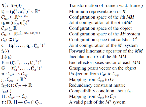
Consider multiple MMs (
 ${M}^3$
) manipulating an object in Figure 4. Let
 $O_wX_wY_wZ_w$
,
 $O_{obj}X_{obj}Y_{obj}Z_{obj}$
,
 $O_{b,i}X_{b,i}Y_{b,i}Z_{b,i}$
and
 $O_{e,i}X_{e,i}Y_{e,i}Z_{e,i}$
be the frames of the world, the object, the mobile base and the end effector of the
 $i$
th MM, where
 $i = 1,2,\ldots ,n$
and
 $n$
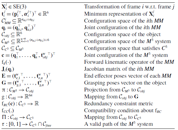
is the number of the robots in the system. Some important notations are listed in Table II for convenience.
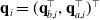
The configurations of the
 $i$
th mobile robot and manipulator are represented as
 $\mathbf{q}_{b,i}\in \mathbb{R}^{n_{b,i}}$
and
 $\mathbf{q}_{a,i}\in \mathbb{R}^{n_{a,i}}$
, respectively. In most cases,
 $n_{b,i}=3$
, as the holonomic mobile robot can move and rotate in all directions on the ground. Therefore, the configuration space of the
 $i$
th MM can be defined as
 $\mathcal{C}_{MM}^i \subseteq \mathbb{R}^{n_{a,i} + n_{b,i}}$
, which is the set of configurations of the
 $i$
th MM
 $\mathbf{q}_{i} = (\mathbf{q}_{b,i}^{\top }, \mathbf{q}_{a,i}^{\top })^{\top }$
. To represent the homogenous transformation of frame
 $i$
w.r.t. frame
 $j$
, we define
 $\mathbf{X}_i^j \in SE(3)$
and its minimum representation
 $\mathbf{t}_i^j = ({\mathbf{p}_i^j}^{T},{\boldsymbol{\alpha }_i^j}^{T})^{\top } \in \mathbb{R}^6$
, in which
 $\mathbf{p}_i^j$
denotes the relative position, and
 $\boldsymbol{\alpha }_i^j$
denotes a minimum description of orientation. Therefore, the configuration space of the object is defined as
 $\mathcal{C}_{obj} \subseteq \mathbb{R}^6$
, which is the set of the object’s poses with respect to the world frame
 $\mathbf{t}_{obj}^w$
.
Definition of some important notations.
Let the configuration space of the system
 $\mathcal{C}_{M^3} = \mathcal{C}_{MM}^1 \times \ldots \times \mathcal{C}_{ MM}^i \times \ldots \times \mathcal{C}_{MM}^n \times \mathcal{C}_{obj} \subseteq \mathbb{R}^{\sum _{i=1}^{n}{(n_{a,i} + n_{b,i})+6}}$
be the set of
 $\mathbf{c} = (\mathbf{q}_1^{\top }, \ldots , \mathbf{q}_i^{\top }, \ldots , \mathbf{q}_n^{\top }, {\mathbf{t}_{obj}^w}^{\top })^{\top }$
. The forward kinematics of the
 $i$
th MM at position-level and velocity-level are defined as Eq. (1) and Eq. (2), respectively.
 \begin{equation} \mathbf{t}{_{e,i}^w} = \mathrm{f}_k(\mathbf{q}_{i}) \end{equation}
 \begin{equation} \dot {\mathbf{t}}{_{e,i}^w} = \frac {\partial {\mathrm{f}_k(\mathbf{q}_{i})}} {\partial {\mathbf{q}_{i}}} \dot {\mathbf{q}}_i = \mathbf{J}_i(\mathbf{q}_{i}) \dot {\mathbf{q}}_i \end{equation}
where
 $\mathrm{f}_k(.)$
is the forward kinematic operator, and
 $\mathbf{J}_i(\mathbf{q}_{i}) \in \mathbb{R}^{6 \times ({n_{a,i} + n_{b,i}})}$
is the analytical Jacobian matrix of the
 $i$
th MM. When a six-
 $\textit {DOF}$
(degree of freedom) manipulator is mounted on an omnidirectional mobile robot, the column of
 $\mathbf{J}_i(\mathbf{q}_{i})$
is larger than that of the row, leading to redundancy of the MM.
2.2. Closed-chain constraint
In the proposed framework and the experiments, we make the following assumptions:
Assumption 1:
-
• The object is rigid and its geometric information is known;
-
• The grasping pose w.r.t. the object’s pose is constant and known;
-
• There is no slippage and deformation between the end effector and the object;
-
• The model of the robots and the scene are known in advance.
Given a random sample
 $\mathbf{c} = (\mathbf{q}_1^{\top }, \ldots , \mathbf{q}_i^{\top }, \ldots , \mathbf{q}_n^{\top }, {\mathbf{t}_{obj}^w}^{\top })^{\top }$
, we define the vector of the end effector’s poses as
 $\mathbf{E} = (\mathbf{t}{_{e,1}^w}^{\top },\ldots , \mathbf{t}{_{e,i}^w}^{\top }, \ldots , \mathbf{t}{_{e,n}^w}^{\top })^{\top } \in \mathbb{R}^{6n}$
where
 $\mathbf{t}{_{e,i}^w} = \mathrm{f}_k(\mathbf{q}_{i})$
. The vector of the grasping poses on the object is denoted as
 $\mathbf{G} = (\mathbf{t}{_{g,1}^w}^{\top },\ldots , \mathbf{t}{_{g,i}^w}^{\top }, \ldots , \mathbf{t}{_{g,n}^w}^{\top })^{\top } \in \mathbb{R}^{6n}$
, in which
 $\mathbf{t}{_{g,i}^w}$
represents the
 $i$
th grasping pose w.r.t. the world frame. For convenience, a projection
 $\unicode {x03C0}\,:\, \mathcal{C}_{M^3} \rightarrow \mathcal{C}_{obj}$
is defined so that
 $\unicode {x03C0}(\mathbf{c}) = \mathbf{t}_{obj}^w$
. According to Assumption 1,
 $\mathbf{G}$
can be easily derived by the geometric transformation
 $g\,:\, \mathcal{C}_{obj} \rightarrow \mathbb{R}^{6n}$
.
 \begin{equation} \mathbf{G} = g(\unicode {x03C0}(\mathbf{c})) \end{equation}
When rigid grasp exists between
 $\mathbf{t}{_{e,i}^w}$
and
 $\mathbf{t}{_{g,i}^w}$
for all
 $i = 1,2,\ldots ,n$
, the closed-chain constraint (
 ${C}^3$
) forms, and it can be formally described by
 $\mathrm{f}_{C^3}\,:\, \mathcal{C}_{M^3} \rightarrow \mathbb{R}^{6n}$
in Eq. (4).
 \begin{equation} \mathrm{f}_{C^3}(\mathbf{c}) = \mathbf{E} - \mathbf{G} =\boldsymbol{0} \end{equation}
Therefore, the set of configurations that satisfy the closed-chain constraint is denoted as
 $\mathcal{C}_{C^3} \subseteq \mathcal{C}_{M^3}$
in Eq. (5).
 \begin{equation} \mathcal{C}_{C^3} = \{ \mathbf{c} | \mathbf{c} \in \mathcal{C}_{M^3}, \mathrm{f}_{C^3}(\mathbf{c}) = \boldsymbol{0} \} \end{equation}
2.3. Redundancy constraint
Redundancy is a double-edged sword. On the one hand, it allows the MM to keep desired configuration while following specified end effector path. On the other hand, it brings additional constraints to the motion planning problem. The fundamental difference between the closed-chain constraint and the redundancy constraint (RC) is that
 ${C}^3$
is “hard” but RC is “soft,” in which “hard” constraints have to be satisfied exactly everywhere, and “soft” constraints are usually described by cost functions and optimized as much as possible. Therefore, RC can be transformed into an optimization problem and formally defined as follows.
 \begin{equation} \begin{aligned} &\arg \max _{\mathbf{c}} \quad \mathrm{f}_{RC}(\mathbf{c})\\ &\begin{array}{r@{\quad }r@{}l@{\quad }l} s.t. &\mathbf{c} \in \mathcal{C}_{C^3}\cap \mathcal{C}_{free} \end{array} \end{aligned} \end{equation}
where
 $\mathcal{C}_{free}$
represents the set of collision-free configurations with appropriate dimensions.
 $\mathrm{f}_{RC}\,:\, \mathcal{C}_{C^3} \rightarrow \mathbb{R}$
is the normalized RC metric of the system and will be introduced in Section 3.3.
2.4. Problem definition
In addition to the notations above, we define a mapping
 $\Pi \;:\; \mathcal{C}_{obj} \rightarrow \mathcal{C}_{C^3}$
so that given a pose of the object
 $\mathbf{t}_{obj}^w$
,
 $\Pi (\mathbf{t}_{obj}^w) = \{ \mathbf{c} | \mathbf{c} \in \mathcal{C}_{C^3}\cap \mathcal{C}_{free}, \unicode {x03C0}(\mathbf{c}) = \mathbf{t}_{obj}^w \}$
. It is the set of configurations that satisfy collision and closed-chain constraints while the object’s pose is invariant. Therefore, the motion planning of multiple MMs under closed-chain, redundancy, and obstacle-avoidance constraints is defined as follows: given the world model
 $\mathcal{W}$
, a start configuration
 $\mathbf{c}_{start} \in \mathcal{C}_{C^3}\cap \mathcal{C}_{free}$
and a target pose of the object
 $\mathbf{t}_{obj}^w$
, find a path
 $\unicode {x03C4}\;:\; [0,1] \rightarrow \mathcal{C}_{C^3}\cap \mathcal{C}_{free}$
such that 1)
 $\unicode {x03C4}(0) = \mathbf{c}_{start}$
; 2)
 $\unicode {x03C4}(1) \in \Pi (\mathbf{t}_{obj}^w)$
; and 3)
 $\mathrm{f}_{RC}(\mathbf{c})$
is maximized throughout
 $\unicode {x03C4}$
. The mathematical expression is shown in Eq. (7).
 \begin{equation} \begin{array}{cl} \text{ find } & \unicode {x03C4}\;:\; [0,1] \rightarrow \mathcal{C}_{C^3}\cap \mathcal{C}_{free} \subseteq \mathbb{R}^{6+\sum _{i=1}^{n}{(n_{a,i} + n_{b,i})}} \\[4pt] \text{ s.t. } & \unicode {x2460} \ \unicode {x03C4}(0) = \mathbf{c}_{start} \\[4pt] & \unicode {x2461} \ \unicode {x03C4}(1) \in \Pi (\mathbf{t}_{obj}^w) \\[4pt] & \unicode {x2462} \ \arg \max \limits _{\mathbf{c}} \ \mathrm{f}_{RC}(\mathbf{c}) \end{array} \end{equation}
3. Semi-coupled hierarchical motion planning framework
3.1. Overview of the framework
One challenge of the motion planning problem is the high-dimensional configuration space. As discussed in Section 1.1, to satisfy the closed-chain constraint of the system, PJ-like centralized frameworks will project a random state
 $\mathbf{c}_{rand} = (\mathbf{q}_1^{\top }, \ldots , \mathbf{q}_i^{\top }, \ldots , \mathbf{q}_n^{\top }, {\mathbf{t}_{obj}^w}^{\top })^{\top } \in \mathcal{C}_{M^3}$
to a new state
 $\mathbf{c}_{new} \in \mathcal{C}_{C^3}$
iteratively. Assuming there are
 $n$
robots and the object is required to achieve six-dimensional motion in the workspace, the size of the closed-chain constrained Jacobian
 $\mathbf{J}_{C^3}(\mathbf{c})$
will be
 $6n \times \left (\sum _{i=1}^{n}{(n_{a,i} + n_{b,i})+6}\right )$
(see Appendix B). According to Appendix C, the time and space complexity when calculating the pseudo-inverse of
 $\mathbf{J}_{C^3}(\mathbf{c})$
are
 $\mathcal{O}_t(n^3)$
and
 $\mathcal{O}_s(n^2)$
, respectively. Therefore, when
 $n$
increases, the projection process (see Appendix A) will be extremely slow and easy to fall into local minima.
Another challenge of solving Eq. (7) is the coupling between closed-chain and RCs. Ideally, it is necessary to optimize the RC metric on each sample
 $\mathbf{c}$
and generate a globally optimal path about
 $\mathrm{f}_{RC}(\mathbf{c})$
. However, this is hard to achieve both technically and theoretically. On the one hand, most samples are not on the final path connecting
 $\unicode {x03C4}(0)$
and
 $\unicode {x03C4}(1)$
, hence optimizing
 $\mathrm{f}_{RC}(\mathbf{c})$
on these samples is unnecessary and time-consuming. On the other hand, the convergence to optimality is not guaranteed for the existing optimal motion planners like
 ${RRT}^*$
[Reference Karaman and Frazzoli26] when optimizing over something other than the path length.
Therefore, we decompose Eq. (7) into the following two layers. Collision-free object’s path is first planned in Eq. (8), then the configuration of each robot is optimized in Eq. (9).
 \begin{equation} \begin{array}{cl} \text{ find } & \unicode {x03C4}'\;:\; [0,1] \rightarrow \mathcal{C}_{obj} \cap \mathcal{C}_{free} \subseteq \mathbb{R}^{6} \\[5pt] \text{ s.t. } & \unicode {x2460} \ \unicode {x03C4}'(0) = \mathbf{t}_{start} \\[5pt] & \unicode {x2461} \ \unicode {x03C4}'(1) = \mathbf{t}_{goal} \\[5pt] & \begin{cases} \unicode {x2462} \ \exists \mathbf{q}_{i} \in \mathcal{C}_{free}, \ \ni \mathrm{f}_k(\mathbf{q}_i)-\mathbf{t}_{g,i}^w = \boldsymbol{0} \\[5pt] \unicode {x2463} \ \mathrm{f}_{CC}(\mathrm{f}_{RC,i}(\mathbf{q}_i)) \end{cases} \end{array} \end{equation}
 \begin{equation} \begin{array}{c@{\quad}l} \arg \max \limits _{\mathbf{q}_i} & \mathrm{f}_{RC,i}(\mathbf{q}_i) \\[4pt] \text{ s.t. } & \mathbf{q}_i \in \mathbb{R}^{n_{a,i}+n_{b,i}} \cap \mathcal{C}_{free} \\[4pt] & \mathrm{f}_k(\mathbf{q}_i)-\mathbf{t}_{g,i}^w = \boldsymbol{0} \end{array} \end{equation}
To alleviate the time cost brought by the high-dimensional configuration space, task space decomposition is applied to quickly check the closed-chain constraint. In condition
 $\unicode {x2462}$
of Eq. (8), given the grasping pose
 $\mathbf{t}_{g,i}^w$
, to meet the closed-chain constraint, each robot only need to project its own joint configuration
 $\mathbf{q}_i$
based on
 $\mathbf{J}_i(\mathbf{q}_{i})$
other than
 $\mathbf{J}_{C^3}(\mathbf{c})$
. According to Appendix C, the time and space complexity when calculating the pseudo-inverse of
 $\mathbf{J}_i(\mathbf{q}_{i}) (i=1,\ldots ,n)$
are
 $\mathcal{O}_t(n)$
and
 $\mathcal{O}_s(n)$
, respectively. Therefore, the computation complexity will be reduced compared with PJ-like centralized frameworks.
To alleviate the challenge brought by the coupling between closed-chain and RCs, the motion of the object and the robots is planned asynchronously. In addition, collision and closed-chain of the
 $i$
th MM (condition
 $\unicode {x2462}$
) and the compatibility condition (CC) about
 $\mathrm{f}_{RC,i}(\mathbf{q}_i)$
(condition
 $\unicode {x2463}$
) are checked to avoid conflict between the two layers.
The framework composed by Eq. (8) and Eq. (9) is unified since different mapping
 $\mathrm{f}_{CC}(.)$
will lead to different motion planners. When condition
 $\unicode {x2462}$
exists and
 $\mathrm{f}_{CC}(.)\,:\!=\,\arg \max _{{\mathbf{q}_i}} \mathrm{f}_{RC,i}(\mathbf{q}_i)$
, where
 $\mathrm{f}_{{ RC},i}(\mathbf{q}_{i})$
is the normalized RC metric of the
 $i$
th MM, Eq. (8) will plan the object’s moiton and optimize the joint configuration simultaneously; hence, Eq. (9) is no longer necessary, and this will lead to a fully centralized planner. When conditions
 $\unicode {x2462}$
and
 $\unicode {x2463}$
in Eq. (8) do not exist, this is actually a fully decoupled framework, which is similar to [Reference Hekmatfar, Masehian and Mousavi28]. When condition
 $\unicode {x2462}$
exists and
 $\mathrm{f}_{CC}(.)\,:\!=\,\mathrm{f}_{RC,i}(\mathbf{q}_i) \gt {thres}$
, where
 ${thres} \in [0,1]$
is a threshold of
 $\mathrm{f}_{RC,i}(\mathbf{q}_i)$
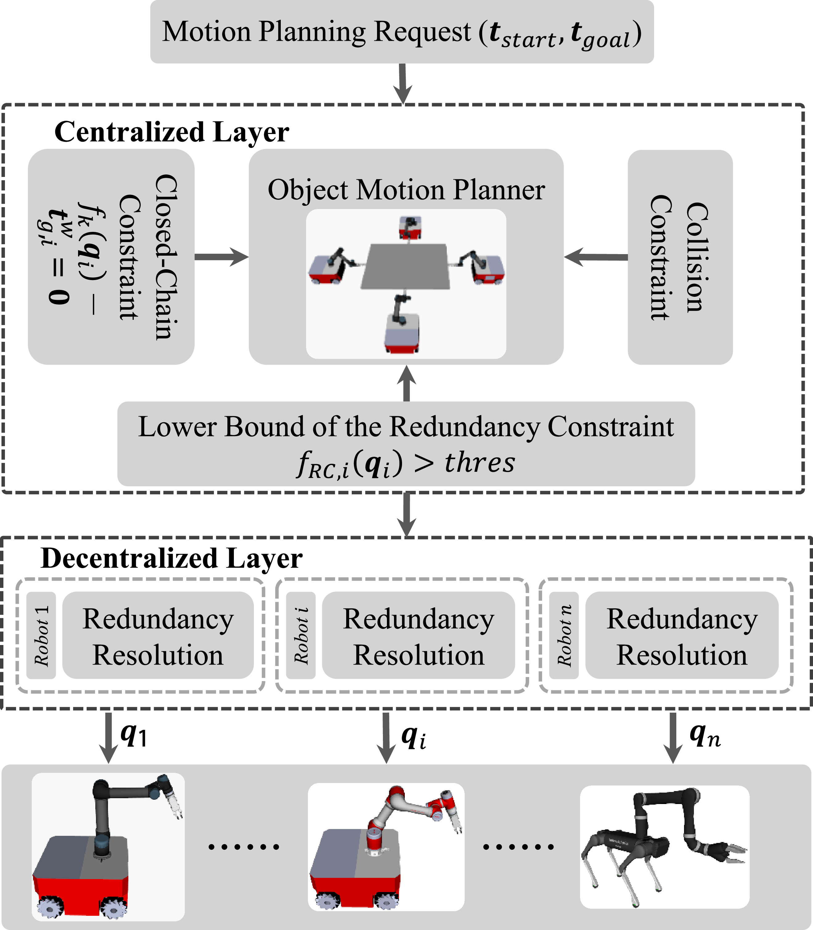
, this will lead to a semi-coupled framework, which is shown in Figure 3.
Overview of the semi-coupled hierarchical framework.
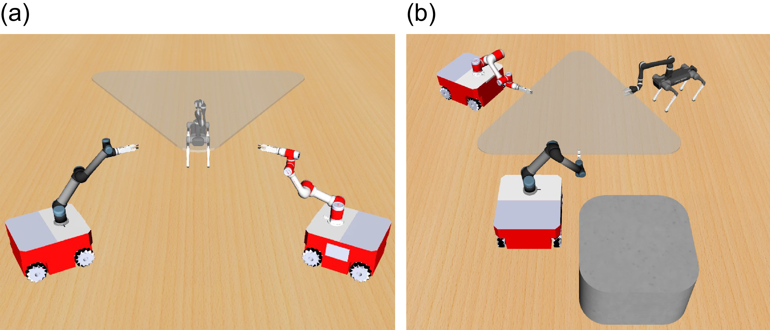
Multiple mobile manipulators system. The object should be transported while avoiding collision and obeying the closed-chain constraint.

In the semi-coupled framework, the “soft” RC is relaxed in the first layer and delayed to the next layer for optimization. The parameter thres can be seen as a coupling factor. As it approaches maximum value 1, the coupling between the two layers gradually intensifies, which will bring more computational burden to Eq. (8). As it approaches minimum value 0, the two layers gradually decouple, which may cause conflict between them. Therefore, thres should be carefully selected so that the compatibility between the two layers is ensured while not putting much computation burden on the former. The detail of the two layers is introduced in the following.
3.2. Centralized layer – object motion planner
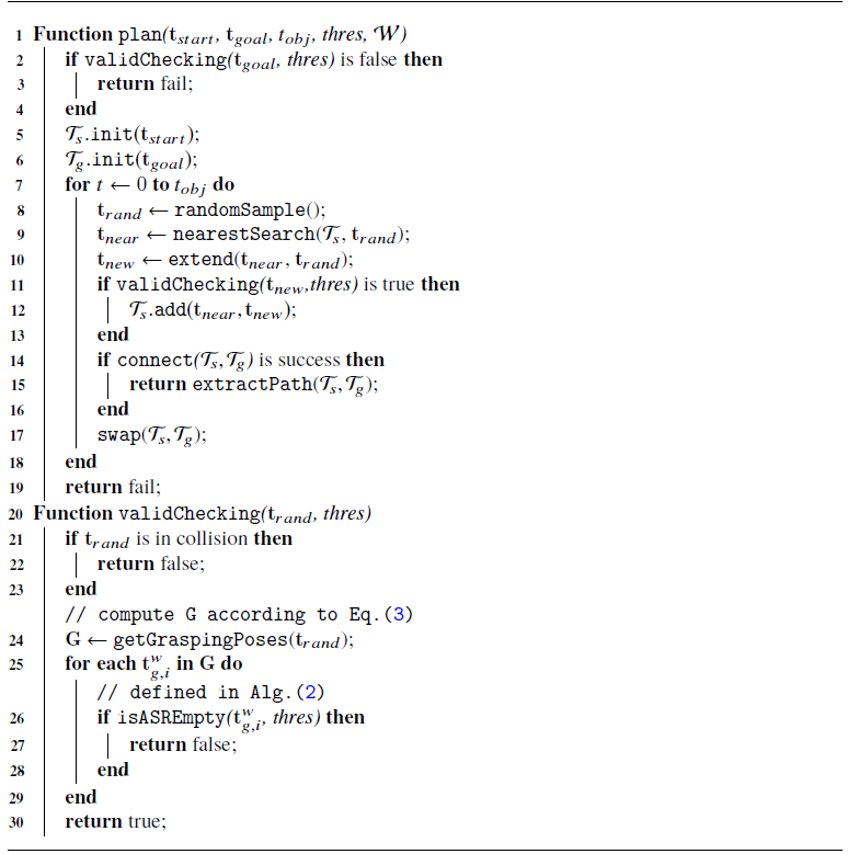
Alg. 1 shows the object’s motion planner in the structure of RRTConnect algorithm [Reference Kuffner and LaValle30]. By encapsulating the validity checking module, which checks collision, closed-chain, and lower bound of the RC metric, into an independent component, working with other sampling-based algorithms, such as PRM [Reference Kavraki, Svestka, Latombe and Overmars27] and EST [Reference Hsu, Latombe and Motwani29], is also possible. For brevity of notations, we omit the superscript and subscript of
 $\mathbf{t}_{obj}^w$
in this part. For example,
 $\mathbf{t}_{start}$
,
 $\mathbf{t}_{goal}$
, and
 $\mathbf{t}_{rand}$
represent the start, the goal, and random pose of the object w.r.t. the world frame, separately. The key functions in Alg. 1 are explained as follows:
-
•
 $\texttt {plan}(\mathbf{t}_{start}, \mathbf{t}_{goal}, t_{obj}, \textit {thres}, \mathcal{W})$
generates collision-free object’s path when the planning request (
$\mathbf{t}_{start}, \mathbf{t}_{goal}$
), allowed planning time
$t_{obj}$
and the world model
$\mathcal{W}$
are specified. Before planning, the validity of
$\mathbf{t}_{goal}$
is first checked, and two trees are initialized, where
$\mathcal{T}_s$
starts from
$\mathbf{t}_{start}$
and
$\mathcal{T}_g$
starts from
$\mathbf{t}_{goal}$
. Then a random object’s pose
$\mathbf{t}_{rand}$
and its nearest neighbor
$\mathbf{t}_{near}$
on
$\mathcal{T}_s$
are computed. After that, a new node
$\mathbf{t}_{new}$
is generated from
$\mathbf{t}_{near}$
to
$\mathbf{t}_{rand}$
along the given step size. When
$\mathbf{t}_{new}$
is valid, the edge connecting
$\mathbf{t}_{near}$
and
$\mathbf{t}_{new}$
will be added to
$\mathcal{T}_s$
. In each iteration, the two trees try to connect with each other and extract the valid path. If the two trees are unable to connect, they are swapped and continue to grow in the next iteration until the path is found or the allowed time
$t_{obj}$
is exceeded.
-
•
$\texttt {validChecking}(\mathbf{t}_{rand}, \textit {thres})$
checks whether
$\mathbf{t}_{rand}$
can be extended to a composite configuration
$\mathbf{c}_{rand} \in \mathcal{C}_{C^3}\cap \mathcal{C}_{free}$
so that
$\unicode {x03C0}(\mathbf{c}_{rand}) = \mathbf{t}_{rand}$
and
$\mathrm{f}_{RC}(\mathbf{c})$
is larger than thres. When the object is collision-free, the grasping poses vector
$\mathbf{G}$
will be calculated based on Eq. (3). For each pose
$\mathbf{t}_{g,i}^w$
in
$\mathbf{G}$
, the allowed sampling region is sampled to check whether the closed-chain, collision and the user-specified lower bound of the RC metric can be satisfied for each MM. When these conditions are met for all
$i = 1,2,\ldots ,n$
,
$\mathbf{t}_{rand}$
is seen as a valid sample. The detail of
$\texttt {isASREmpty()}$
is introduced in the following.









Object Motion Planner

Allowed Sampling Region: In the hierarchical framework, the compatibility between adjacent layers should be carefully considered. Otherwise, the centralized layer may conflict with the decentralized layer. For example, although the object’s pose is collision-free in Figure 2(a), it exceeds the workspace of the robots, and the closed-chain constraint is unable to be satisfied. Similarly, for the object’s pose in Figure 2(b), although a configuration can be found to satisfy the closed-chain constraint, one of the robots must be in an awkward configuration due to obstacles. Therefore, the object’s poses in these cases should be abandoned as they are inexecutable or lead to poor and unstable joint configuration in the decentralized layer.
To check the validity of
 $\mathbf{t}_{g,i}^w$
, we define the allowed sampling region (ASR) for each mobile robot in Eq. (10).
 \begin{equation} \begin{split} ASR(\mathbf{t}_{g,i}^w, & \textit {thres}) = \{ \mathbf{q}_{b,i} \ | \ \exists \mathbf{q}_{a,i}, \ni \mathrm{f}_k(\mathbf{q}_{i}) = \mathbf{t}_{g,i}^w \\ & \ \textit {and} \ \mathrm{f}_{{RC},i}(\mathbf{q}_{i}) \geq \textit {thres} \ \textit {and} \ \mathbf{q}_{i} \in \mathcal{C}_{free} \} \end{split} \end{equation}
where
 $\mathrm{f}_{{RC},i}(\mathbf{q}_{i})$
is the normalized RC metric of the
 $i$
th MM, and
 $thres$
is a user-specified threshold of this metric.
 $\mathrm{f}_{{RC},i}(\mathbf{q}_{i})$
is a component of
 $\mathrm{f}_{RC}(\mathbf{c})$
, and their expressions are defined in Eq. (11) and Eq. (12). Therefore, we can check whether existing
 $\mathbf{q}_{b,i} \in ASR(\mathbf{t}_{g,i}^w, {thres})$
to see the validity of
 $\mathbf{t}_{g,i}^w$
.
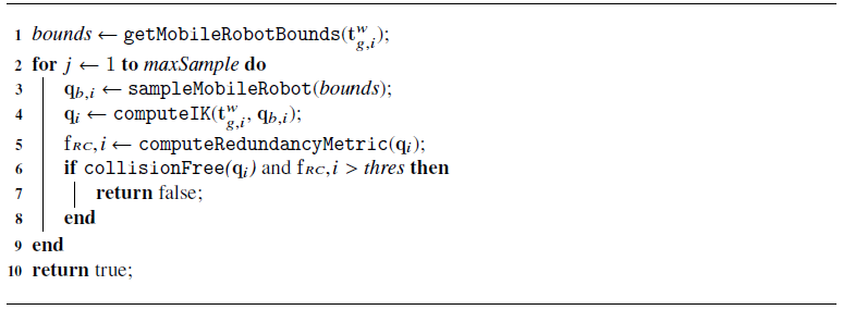
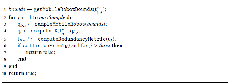
isASREmpty(t g, i w , thres)
ASR varies with the grasping pose
 $\mathbf{t}_{g,i}^w$
and the threshold thres, and it constitutes the most computationally expensive step in Algorithm 1. Its computation time is influenced by both the number of robots and the complexity of the environment. Theoretically, in a fixed scene, the required time grows linearly with the number of robots. In cluttered environments with more obstacles, the probability of obtaining a valid ASR decreases, leading to a significant increase in computation time. Due to the high complexity of the system, ASR is typically approximated via sampling.
In cooperative transportation tasks, the mobile robot has almost unlimited range of motion on the ground but the manipulator only has limited reachable workspace, which can be seen as heuristic information. In Alg. 2, given the grasping pose
 $\mathbf{t}_{g,i}^w$
, we can get the approximate motion bounds for the mobile robot based on the maximum workspace of the manipulator, and this idea has been applied for the MM in the literature [Reference Zhang, Sheng, Sun, Sheng, Xiong and Zhu14], [Reference Thakar, Rajendran, Kabir and Gupta8]. Then, given a random
 $\mathbf{q}_{b,i}$
within bounds, the joint configuration of the MM
 $\mathbf{q}_i$
can be computed based on the iterative inverse kinematic solvers. Finally, if
 $\mathbf{q}_i$
is not in collision and the corresponding RC metric
 $\mathrm{f}_{{RC},i}(\mathbf{q}_{i})$
is larger than thres, the set
 $ASR(\mathbf{t}_{g,i}^w, \textit {thres})$
is not empty and
 $\mathbf{t}_{g,i}^w$
can be seen as a valid grasping pose.
3.3. Decentralized layer – redundancy resolution
As shown in Figure 3 and Eq. (8)-(9), redundancy resolution is an independent component in the semi-coupled hierarchical framework, and various off-the-shelf algorithms can be used in the decentralized layer. For example, our previous work [Reference Zhang, Sheng, Hu, Sheng, Xiong and Zhu24] proposed a real-time and robust redundancy resolution for the MM in the human–robot cooperative transportation task, hence we will reuse this algorithm and briefly introduce it in the following. However, as long as the RC is modeled as an optimization problem, such as [Reference Fabregat-Jaén, Peidró, Colombo, Rocco and Reinoso12], it can be combined with the proposed framework.
The key to the redundancy resolution is fulfilling additional constraints while obeying the end effector’s motion; hence, the following constraints are introduced for the
 $i$
th MM.
 \begin{equation} \mathrm{f}_{{RC},i}(\mathbf{q}_i) = \mu (\mathbf{q}_i) \times F(\mathbf{q}_i) \times B(\mathbf{q}_i) \end{equation}
where
 $\mu (\mathbf{q}_i)$
,
 $F(\mathbf{q}_i)$
and
 $B(\mathbf{q}_i)$
represent the dexterity of the MM, the formation metric of the MRS and obstacle-avoidance constraint index of the mobile robot, respectively. These indexes are relative values w.r.t. their global optimum, hence are normalized within [0,1].
When they are small, the planner will generate a better configuration in the next round of optimization. For example, when the dynamic obstacles approach the mobile robot,
 $B(\mathbf{q}_i)$
will be punished, and the mobile robot will move far away from the obstacles in the next iteration. An intuitive explanation of Eq. (11) is as follows. As a redundant robot, there are extra DOF to fulfill the user-specified constraints. In cooperative transportation task, the MM should adjust self-motion to avoid obstacles on the ground and keep a dexterous configuration and optimize the formation of the system as much as possible. For more detail, please refer to [Reference Zhang, Sheng, Hu, Sheng, Xiong and Zhu24].
Therefore, the RC metric of the system
 $\mathrm{f}_{RC}(\mathbf{c})$
in Eq. (6) can be defined as the minimum
 $\mathrm{f}_{{RC},i}(\mathbf{q}_i)$
of all robots. When
 $\mathrm{f}_{{RC},i}(\mathbf{q}_i)$
reaches its maximum for all robots, the redundancy of the system is optimized.
 \begin{equation} \mathrm{f}_{RC}(\mathbf{c}) = {min}\{\mathrm{f}_{{RC},i}(\mathbf{q}_i) | 1 \leq i \leq n \} \end{equation}
In the simulation and real-world experiments, Nelder-Mead simplex algorithm [Reference Nelder and Mead31] is chosen as the real-time solver to get optimal joint configuration
 $\mathbf{q}_i$
about
 $\mathrm{f}_{{RC},i}(\mathbf{q}_i)$
. It has no requirement on the differentiability of
 $\mathrm{f}_{{RC},i}$
and shows good performance in practice.
4. Simulation and experimental results
4.1. Experimental setup
To demonstrate the superiority of the proposed framework, numerous experiments are conducted in Section 4.2 and Section 4.3, respectively. Moreover, different numbers of robots are considered in the experiments. The computer is Intel i7-8700 (3.2 GHz) with 32 GB of memory.
According to Assumption 1,
 $\mathrm{f}_k(\mathbf{q}_i)$
in Eq. (1) and
 $g(\mathbf{t}_{obj}^w)$
in Eq. (3) can be derived from the geometric model of the MRS.
 $\mathrm{f}_{CC}(.)$
in Eq. (8) is set to
 $\mathrm{f}_{RC,i}(\mathbf{q}_i) \gt {thres}$
to couple the two layers. The convergence criteria for the projection process are set to 0.005 in SCHF, which works well in the experiment. The expression of
 $\mathrm{f}_{RC,i}(\mathbf{q}_i)$
is shown in Eq. (11) and the suitable value of thres will be tested and discussed in Section 4.2.5.
4.2. Performance of the semi-coupled hierarchical framework
4.2.1. Simulation scene
As obstacles or the number of robots increase, the scenes are shown in Figure 5(a)–(f). The size of the scenes is
 $15m \times 25m$
. The start and goal states are displayed on the most left and most right, respectively. Snapshots during the tasks are also shown in Figure 5. The pictorial motion is available in the attached video. In these tasks, the start and goal states are assumed to satisfy the closed-chain and collision constraints, and valid paths connecting the start and goal states exist theoretically. Moreover, the height of some obstacles is lower than the maximum allowed height of the object, which means that obstacles may be crossed by the system.
4.2.2. Simulation 1
In this simulation, we compare the proposed framework with centralized frameworks, such as PJ [Reference Yakey, LaValle and Kavraki16], [Reference Berenson, Srinivasa and Kuffner17], AT [Reference Jaillet and Porta19], and TB [Reference Kim, Um, Suh and Park20]. As discussed in Section 1.1, PJ computes the Jacobian of the system and projects a random sample
 $\mathbf{c}$
onto the manifold based on Newton procedure (see Appendix). AT and TB are built on top of PJ with some modifications. For the fairness of the comparison, in the semi-coupled hierarchical framework (SCHF), the inverse kinematic solver is also chosen as an iterative algorithmalgorithm.
In the tasks shown in Figure 5(a)–(f), the start state
 $\mathbf{t}_{start}$
and goal state
 $\mathbf{t}_{goal}$
of the object are specified by the user. However, in PJ, AT, and TB, not only the state of the object but also the state of the robots should be specified. Therefore, a random goal state
 $\mathbf{c}_{goal}$
will be selected for each scene so that
 $\mathbf{c}_{goal} \in \mathcal{C}_{C^3}\cap \mathcal{C}_{free}$
and
 $\unicode {x03C0}(\mathbf{c}_{goal}) = \mathbf{t}_{goal}$
. Moreover, redundancy can not be resolved directly in PJ, AT, and TB; hence, only closed-chain and collision constraints are considered in these centralized frameworks. PJ, AT, and TB on the multiple MMs system are developed based on
 $OMPL$
[Reference Sucan, Moll and Kavraki32], which is a famous sampling-based motion planning software.
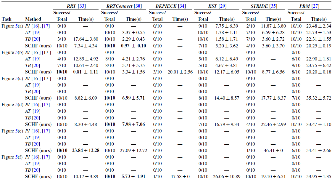
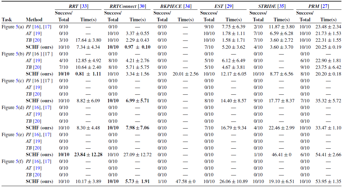
The performances of different frameworks are shown in Table III. The terms and settings are explained as follows. The maximum allowed planning time
 $t_{obj}$
in Alg. 1 is set to
 $20s$
,
 $20s$
,
 $30s$
,
 $30s$
,
 $50s$
, and
 $50s$
for the tasks in Figure 5(a)–(f), respectively. maxSample in Alg. 2 is set to 200, and
 $thres$
is set to 0.4 to couple the centralized and decentralized layers. Each framework is combined with six random planning algorithms, namely
 $RRT$
[Reference LaValle33],
 $RRTConnect$
[Reference Kuffner and LaValle30],
 $BKPIECE$
[Reference Şucan and Kavraki34],
 $EST$
[Reference Hsu, Latombe and Motwani29],
 $STRIDE$
[Reference Gipson, Moll and Kavraki35,] and
 ${PRM}$
[Reference Kavraki, Svestka, Latombe and Overmars27]. Please notice that sampling-based motion planners like
 $RRT$
are sub-modules of the proposed framework and are only used to search the object’s motion rather than the MM’s joint motion. Each combination runs 10 times to get the statistical results. “Success/Total” columns represent the successful and total simulations conducted. “Time(s)” columns correspond to the mean and standard deviation of the path computation time for the system, measured over multiple trials. When all simulations fail, “Time(s)” columns are set to “—.”
As shown in Figure 5 and Table III, the performance of PJ, AT, and TB improves sequentially across these tasks. All three methods perform satisfactorily in simple scenarios, such as the one depicted in Figure 5(a). However, their performance deteriorates noticeably as obstacle density increases. Furthermore, we observe that PJ-like frameworks are highly sensitive to hyper-parameters during code debugging – such as the constraint tolerance in PJ and the maximum chart validity radius in AT and TB – imposing additional tuning burden on developers.
According to Table III, the proposed framework significantly outperforms PJ-like centralized frameworks. This advantage stems from our hierarchical approach to planning object and robot motions, whereas PJ-like frameworks plan all system motions simultaneously. In addition,
 $RRTConnect$
(a variant of
 $RRT$
) demonstrates the best performance when integrated with our framework, and is therefore selected as the default motion solver in subsequent experiments.
Comparison of the semi-coupled hierarchical framework (SCHF) with centralized frameworks (PJ [Reference Yakey, LaValle and Kavraki16], [Reference Berenson, Srinivasa and Kuffner17], AT [Reference Jaillet and Porta19] and TB [Reference Kim, Um, Suh and Park20]).
4.2.3. Simulation 2
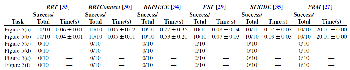
In this simulation, we compare the proposed framework with the fully decoupled hierarchical framework. When the closed-chain constraint and the lower bound of the RC metric are not guaranteed in Figure 3, the centralized layer and the decentralized layer become fully decoupled, resulting in a framework similar to [Reference Hekmatfar, Masehian and Mousavi28]. The performance of the decoupled framework in the tasks in Figure 5(a)–(f) is shown in Table IV.
(a)–(f). Simulation scenes range from simple to complex. The size of the scenes is
 $15m \times 25m$
. Robot models are snapshots during the tasks. The height of some obstacles is lower than the maximum allowed height of the object, hence obstacles may be crossed by the system like the path in (b)–(f).

As illustrated in Figure 5(a)–(b), the centralized and decentralized layers remain largely compatible in simple scenarios with straightforward tasks, making it possible to omit explicit verification of the closed-chain constraint and the lower bound on the RC metric. Under such conditions, the decoupled framework performs effectively. However, as environmental complexity increases with the introduction of obstacles, the motion planning problem becomes more challenging, often leading to conflicts between the two layers. Consequently, as shown in Figure 5(c)–(f), the performance of the decoupled framework degrades significantly. A representative failure case is depicted in Figure 6, although the object’s trajectory remains collision-free, the method in [Reference Hekmatfar, Masehian and Mousavi28] fails to generate feasible paths for the robots that simultaneously satisfy collision avoidance, closed-chain, and RCs.
4.2.4. Simulation 3
In this simulation, we compare the proposed framework with algorithms based on the virtual structure. In [Reference Tang, Zhang, Yu and Zhang22, Reference Alonso-Mora, Baker and Rus23, Reference Jiao, Cao, Gu, Nahavandi, Yang and Tan25], the object and the robots are encircled by polygons on the ground. As long as the virtual structure intersects with obstacles, the system is considered in collision. Therefore, the obstacle-avoidance strategy is conservative. Take the task in Figure 5(b) as an example. Our motion planner is able to find a shorter path that crosses obstacles. However, the path in Figure 5(b) becomes infeasible for [Reference Tang, Zhang, Yu and Zhang22, Reference Alonso-Mora, Baker and Rus23, Reference Jiao, Cao, Gu, Nahavandi, Yang and Tan25], and they can only find a longer path that bypasses obstacles, which is shown in Figure 1. Crossing obstacles is an essential ability for the multiple-robots system and will increase the success rate of the motion planner in cluttered environments.
Performance of the fully decoupled hierarchical framework [Reference Hekmatfar, Masehian and Mousavi28].
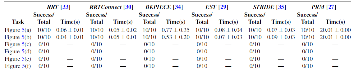
Performance of different thres in the semi-coupled hierarchical framework.

4.2.5. Simulation 4
In this simulation, we test the effects of the coupling factor thres on the SCHF. The time cost and success rate in different tasks are shown in Table V and explained in the following.
When thres = 0, SCHF performs well in Figure 5(a)–(b). As the scenes become cluttered, such as Figure 5(c)–(f), its performance is poor as the “soft” RC is not considered in the centralized layer, which may cause conflict with the decentralized layer. Notice that closed-chain and collision of the MM (condition
 $\unicode {x2462}$
in Eq. (8)) are always checked in this experiment, hence the time cost in Figure 5(a)–(b) is slightly over the fully decoupled framework (Table IV).
When thres is large, i.e., 0.8 and 1.0, the performance of the SCHF is extremely poor and the reasons are twofold. On the one hand, as thres grows, so does the time cost as the centralized layer has to spend more time to find valid samples when planning the object’s motion. As a result, the success rate will decrease within the limited planning time. On the other hand,
 $\mathrm{f}_{{RC},i}(\mathbf{q}_i)$
is a relative normalized index w.r.t. its global optimum in the entire configuration space. When obstacles and closed-chain exist, the robots may find locally optimal joint configurations but are hard to reach global optimums, hence the success rate will be 0 when thres = 1.0. Furthermore, thres is also affected by the heterogeneity of the robots. For example, the system in Figure 5(b) only includes the same MMs, while Figure 5(a) contains MM with different mechanical structure.
In summary, thres is affected by the definition of
 $\mathrm{f}_{{RC},i}(\mathbf{q}_i)$
, the clutter of the environment/task and the heterogeneity of the robots. This simulation evaluates a possible expression of
 $\mathrm{f}_{{RC},i}(\mathbf{q}_i)$
and also gives a guideline to choose a suitable thres for other kinds of
 $\mathrm{f}_{{RC},i}(\mathbf{q}_i)$
and tasks. A thumb rule is that in scenarios with no or few obstacles, if the requirement of planning time is critical, thres can be set to a small value. In other scenarios, it should be set to a moderate value, e.g., 0.4, to balance the time cost and success rate in the SCHF.
4.3. Real-world experiments
In the real-world experiments, each MM consists of an omnidirectional mobile base and a 6-DOF manipulator, along with a parallel gripper for object grasping. All robots are connected via wireless communication modules on a shared local network to enable efficient coordination. All the codes are implemented in the architecture of
 $ROS$
based on
 $C++$
. A leader–follower control strategy is adopted, in which one robot is designated as the leader and the others act as followers. Under this scheme, the leader plans the global path for the object, while each follower computes its motion relative to the leader. Each robot then independently optimizes its joint motions in real time through redundancy resolution.
In addition, every mobile robot is equipped with a planar laser scanner for self-localization and detection of both static and dynamic obstacles on the ground. During the experiments, we first built an environment map using Cartographer [Reference Hess, Kohler, Rapp and Andor37], and then employed Adaptive Monte Carlo Localization to estimate the pose of each mobile robot within the map. Prior to executing the transportation task, the control gains of each MM were individually tuned to ensure that both the mobile base and the end-effector could accurately and responsively track the desired motion trajectories.
4.3.1. Experiment 1
In this experiment, we extend the proposed framework to the real-world cooperative transportation task. Obstacles include a pedestrian and two slopes with varying angles and heights. The system should transport the object to the destination while avoiding static and dynamic obstacles. The decentralized layer will optimize the joint configuration of the robots in real-time. Snapshots during the task are shown in Figure 7. The trajectories of the object,
 $\mu (\mathbf{q})$
,
 $F(\mathbf{q})$
and
 $B(\mathbf{q})$
of MM1 and MM2 are shown in Figure 8. The motion process is explained as follows.
-
• At t = 0s, the system is far away from obstacles. Both MM1 and MM2 start with an optimal configuration.
-
• From t = 5s to t = 10s, MM1 meets the pedestrian twice. As a redundant robot, it is able to avoid the dynamic obstacle while not affecting the transportation task. As a punishment,
$\mu (\mathbf{q})$
of MM1 is sacrificed (Figure 8(c)). However, when the obstacle moves away,
$\mu (\mathbf{q})$
can be recovered to a high value. -
• From t = 28s to t = 35s, the system adjusts z and roll of the object to suit the height and direction of slope1. Thanks to the real-time redundancy resolution,
$\mu (\mathbf{q})$
,
$F(\mathbf{q})$
and
$B(\mathbf{q})$
of the two robots remain at high values during this period. -
• From t = 49s to t = 55s, the height of the MM1’s and MM2’s end effector decreases and increases, respectively, which means that the system adjusts pitch of the object to suit the height and direction of slope2. During this period, MM2 gradually approaches the boundary of the workspace in z direction, hence
$\mu (\mathbf{q})$
decreases quickly (Figure 8(d)). -
• From t = 75s to t = 80s, the system has crossed all obstacles and then lowers the object to finish the autonomous cooperative transportation task. Finally, the height of the MM2’s end effector decreases, and
$\mu (\mathbf{q})$
returns to a high value.


Robot path planned by the fully decoupled hierarchical framework [Reference Hekmatfar, Masehian and Mousavi28]. Although the motion of the object is collision-free, [Reference Hekmatfar, Masehian and Mousavi28] is unable to find a valid path that satisfies the collision, closed-chain, and redundancy constraints simultaneously.

Scene of the real-world transportation task by two robots.

(a)–(b) Trajectories of the object in the task shown in Figure 9. (c)–(d)
 $\mu (\mathbf{q})$
,
 $F(\mathbf{q})$
and
 $B(\mathbf{q})$
of MM1 and MM2 during the task.

Therefore, multiple robots are able to cooperate with each other to realize the transportation task in cluttered environments, and each robot could plan the optimal joint configuration and track the desired trajectories precisely.
4.3.2. Experiment 2
In this experiment, we conduct the cooperative transportation task by three robots in real-world environment. Obstacles include a pedestrian and a cuboid with a certain height. Other settings are similar to the former experiment. Snapshots during the task are shown in Figure 9, and the pictorial motion is available in the attached video. From this and the former experiments, we can see that multiple robots are able to cooperate with each other to realize the transportation task in cluttered environments. Moreover, each robot could plan the optimal joint configuration and track the desired trajectories precisely.
Scene of the real-world transportation task by three robots.

4.4. Discussions
As illustrated in Figure 3 and Eq. (8)–(9), the proposed framework adopts a semi-coupled hierarchical architecture. Specifically, the centralized layer enforces both the closed-chain constraint and a user-specified lower bound for the RC metric, while the decentralized layer performs real-time optimization of
 $\mathrm{f}_{RC}(\mathbf{c})$
under the condition that
 $\mathrm{f}_{C^3}(\mathbf{c})$
remains satisfied. A key feature of this design is the decoupling among different robots: the decentralized layer operates in a fully distributed manner, enabling independent and real-time redundancy resolution for each robot.
In comparison to fully centralized frameworks – which typically employ numerical projection operators to generate valid samples while simultaneously planning motions for both the object and all robots – our hierarchical structure substantially simplifies motion planning in high-dimensional systems, as experimentally validated in Section 4.2.2. Compared with decoupled frameworks that plan object and robot motions separately, the semi-coupled coordination between our two layers effectively prevents conflicts and enhances overall planning performance, as demonstrated in Section 4.2.3. Furthermore, relative to virtual structure-based algorithms, the proposed planner supports more diverse and efficient obstacle-avoidance behaviors, including bypassing and crossing maneuvers, which is also verified in Section 4.2.4. The proposed framework is applicable to systems comprising different numbers of heterogeneous MMs. To the best of our knowledge, such complex multi-robot applications have not been previously demonstrated in the robotics literature.
5. Conclusions
In this paper, we propose a novel semi-coupled hierarchical framework to deal with the motion planning of multiple MMs and fulfill the cooperative transportation tasks in cluttered environment. The motion of the object is planned in the centralized layer offline. In the decentralized layer, the redundancy of each robot is explored independently in real-time. A user-specified lower bound of the RC metric, closed-chain, and obstacle-avoidance constraints are guaranteed in the centralized layer to ensure the object’s motion is executable in the decentralized layer. The proposed framework simplifies the complex motion planning problem while not violating the constraints. Its success rate and time cost outperform the benchmark motion planners significantly and can be applied to different numbers of heterogeneous MMs, which are verified in the simulated and real-world experiments.
However, our work has several limitations. First, our approach relies on several assumptions – such as object rigidity and the absence of slippage or deformation between the end-effector and the object. During experiments, however, we observed that slippage tends to occur when the object is heavy. Second, relative localization is not always stable, which can lead to pulling or compression forces on the object. In the future, integrating more accurate localization and tactile feedback between the object and the end-effector could help improve system performance.
Supplementary material
The supplementary material for this article can be found at https://.doi.org/10.1017/S0263574725102865.
Author contributions
Zhenhua Xiong and Xiangyang Zhu led the project and proposed the core idea of this paper. Heng Zhang wrote the article and conducted the experiments. Xinjun Sheng, Haoyi Song, and Wenhang Liu helped to conducted the expetiment, performed data analyses and proposed insightful discussions to this work.
Financial support
This work was supported in part by the National Natural Science Foundation of China (U1813224, 51675325) and Ministry of Education China Mobile Research Fund Project (MCM20180703).
Competing interests
There is no conflicts of interest exist.
Ethical approval
Not applicable.
Appendix A. Projection operation for the centralized frameworks
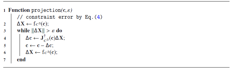
Projection is the basis for the centralized frameworks [Reference Yakey, LaValle and Kavraki16], [Reference Berenson, Srinivasa and Kuffner17], [Reference Jaillet and Porta19], [Reference Kim, Um, Suh and Park20] in Section 4.2.2. Alg. 3 shows the iterative procedure that uses the pseudo-inverse Jacobian matrix of the closed-chain constraint function
 $\mathrm{f}_{C^3}(\mathbf{c})$
.
Projection Through Iteration
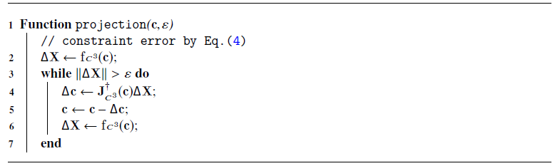
Given a random sample
 $\mathbf{c}$
, Alg. 3 computes the constraint error according to Eq.(4) and compares it with the maximum allowed error
 $\varepsilon$
. When the error is larger than
 $\varepsilon$
, the pseudo-inverse of the constrained Jacobian matrix
 $\mathbf{J}_{C^3}^{\dagger }(\mathbf{c})$
will be calculated to project the random sample by the gradient descent operation.
Appendix B. Constrained Jacobian matrix
In this part, we derive the constrained Jacobian matrix
 $\mathbf{J}_{C^3}(\mathbf{c}) \in \mathbb{R}^{6n \times \left (\sum _{i=1}^{n}{(n_{a,i} + n_{b,i})+6}\right )}$
of the system.
 \begin{equation} \mathbf{J}_{C^3}(\mathbf{c}) = \frac {\partial {\mathrm{f}_{C^3}(\mathbf{c})}}{\partial {\mathbf{c}}} = \frac {\partial {\mathbf{E}} - \partial {\mathbf{G}}}{\partial {\mathbf{c}}} \end{equation}
According to the definition of
 $\mathbf{E}$
and
 $\mathbf{G}$
in Section 2.2,
 $\mathbf{E}$
has no relationship with
 $\mathbf{t}_{obj}^{w}$
, and
 $\mathbf{G}$
has no relationship with
 $\mathbf{q}_i$
. Therefore, Eq. (13) can be simplified to Eq. (14).
 \begin{equation} \frac {\partial {\mathbf{E}} - \partial {\mathbf{G}}}{\partial {\mathbf{c}}} = \left ( \frac {\partial {\mathbf{E}}}{\partial {\mathbf{q}_1}}, \ldots , \frac {\partial {\mathbf{E}}}{\partial {\mathbf{q}_i}}, \ldots , \frac {\partial {\mathbf{E}}}{\partial {\mathbf{q}_n}}, -\frac {\partial {\mathbf{G}}}{\partial {\mathbf{t}_{obj}^w}} \right ) \end{equation}
where
 $\frac {\partial {\mathbf{E}}}{\partial {\mathbf{q}_i}}$
and
 $\frac {\partial {\mathbf{G}}}{\partial {\mathbf{t}_{obj}^w}}$
are defined in Eq. (15) and Eq. (16).
 \begin{align} & \frac {\partial {\mathbf{E}}}{\partial {\mathbf{q}_i}} = \left ( \frac {\partial {\mathrm{f}_k(\mathbf{q}_1)}}{\partial {\mathbf{q}_i}}, \ldots , \frac {\partial {\mathrm{f}_k(\mathbf{q}_i)}}{\partial {\mathbf{q}_i}}, \ldots , \frac {\partial {\mathrm{f}_k(\mathbf{q}_n)}}{\partial {\mathbf{q}_i}} \right )^{\top } \end{align}
 \begin{align} & \frac {\partial {\mathbf{G}}}{\partial {\mathbf{t}_{obj}^w}} = \left ( \frac {\partial {\mathbf{t}_{g,1}^w}}{\partial {\mathbf{t}_{obj}^w}}, \ldots , \frac {\partial {\mathbf{t}_{g,i}^w}}{\partial {\mathbf{t}_{obj}^w}}, \ldots , \frac {\partial {\mathbf{t}_{g,n}^w}}{\partial {\mathbf{t}_{obj}^w}} \right )^{\top } \end{align}
where
 $\frac {\partial {\mathrm{f}_k(\mathbf{q}_j)}}{\partial {\mathbf{q}_i}}$
is given by Eq. (17).
 \begin{equation} \frac {\partial {\mathrm{f}_k(\mathbf{q}_j)}}{\partial {\mathbf{q}_i}} = \begin{cases} \mathbf{J}_i(\mathbf{q}_{i}), & \textit {if} \ i = j \\ \boldsymbol{O}_{6 \times (n_{a,i}+n_{b,i})}, & \textit {if} \ i\neq j \end{cases} \end{equation}
where
 $\mathbf{J}_i(\mathbf{q}_{i})$
is the analytical Jacobian matrix of the
 $i$
th MM.
Suppose the constant homogeneous transformation of frame
 $O_{g,i}X_{g,i}Y_{g,i}Z_{g,i}$
relative to frame
 $O_{obj}X_{obj}Y_{obj}Z_{obj}$
is
 \begin{equation*} \mathbf{X}_{g,i}^{obj} = \left ( \begin{array}{cc} \boldsymbol{R}_{g,i}^{obj} & \mathbf{p}_{g,i}^{obj} \\ \boldsymbol{O}_{1\times 3} & 1 \\ \end{array} \right ).\end{equation*}
Suppose the velocity of a frame is
 $\boldsymbol{\xi } = (\boldsymbol{v}^{\top }, \boldsymbol{\omega }^{\top })^{\top }$
, in which
 $\boldsymbol{v}$
and
 $\boldsymbol{\omega }$
represent the linear and angular velocity of the frame. According to [Reference Caccavale and Uchiyama36], Eq. (18) holds between
 $\boldsymbol{\xi }_{g,i}^w$
and
 $\boldsymbol{\xi }_{obj}^w$
.
 \begin{equation} \boldsymbol{\xi }_{g,i}^w = \left ( \begin{array}{cc} \boldsymbol{I}_{3\times 3} & -S(\mathbf{p}_{g,i}^{w}) \\ \boldsymbol{O}_{3\times 3} & \boldsymbol{I}_{3\times 3} \\ \end{array} \right ) \boldsymbol{\xi }_{obj}^w \end{equation}
where
 $S(.)$
is the skew-symmetric matrix operator. In addition, we use a minimum description to represent the orientation in
 $\mathbf{t}$
, hence Eq. (19) holds between
 $\dot {\mathbf{t}}$
and
 $\boldsymbol{\xi }$
.
 \begin{equation} \boldsymbol{\xi } = \left ( \begin{array}{cc} \boldsymbol{I}_{3\times 3} & \boldsymbol{O}_{3\times 3} \\ \boldsymbol{O}_{3\times 3} & B(\boldsymbol{\alpha }) \\ \end{array} \right ) \dot {\mathbf{t}} \end{equation}
When roll-pitch-yaw angle is used to represent the orientation, we have
 $\boldsymbol{\alpha } = (\phi , \psi , \theta )^{\top }$
and
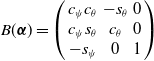 $B(\boldsymbol{\alpha }) = \left ( \begin{array}{ccc} c_{\psi }c_{\theta } & -s_{\theta } & 0 \\ c_{\psi }s_{\theta } & c_{\theta } & 0 \\ -s_{\psi } & 0 & 1 \\ \end{array} \right )$
, where
 $s$
and
 $c$
represent sine and cosine operator, respectively.
Combining Eq. (18) and Eq. (19),
 $\frac {\partial {\mathbf{t}_{g,i}^w}}{\partial {\mathbf{t}_{obj}^w}}$
can be derived in Eq. (20).
 \begin{equation} \frac {\partial {\mathbf{t}_{g,i}^w}}{\partial {\mathbf{t}_{obj}^w}} = \boldsymbol{W}_{i} = \left ( \begin{array}{cc} \boldsymbol{I}_{3\times 3} & -S(\mathbf{p}_{g,i}^{w})B(\boldsymbol{\alpha }_{obj}^w) \\ \boldsymbol{O}_{3\times 3} & -B^{-1}(\boldsymbol{\alpha }_{g,i}^w)B(\boldsymbol{\alpha }_{obj}^w) \\ \end{array} \right ) \end{equation}
Combining Eq. (13)-(17) and Eq. (20),
 $\mathbf{J}_{C^3}(\mathbf{c})$
is finally given in Eq. (21).
 \begin{equation} \mathbf{J}_{C^3}(\mathbf{c}) = \left ( \begin{array}{cccc} \mathbf{J}_1(\mathbf{q}_{1}) & \ldots & \boldsymbol{O} & -\boldsymbol{W}_{0} \\ \vdots & \ddots & \vdots & \vdots \\ \boldsymbol{O} & \ldots & \mathbf{J}_n(\mathbf{q}_{n}) & -\boldsymbol{W}_{n} \\ \end{array} \right ) \end{equation}
Appendix C. Time and space complexity analysis
According to Alg. 3, the most time consuming operation in the iteration process is calculating the pseudo-inverse of the Jacobian matrix. According to the SVD algorithm [Reference Li, Wang and Cai39], for a matrix with dimension
 $p \times q$
, the time complexity and space complexity when calculating the pseudo-inverse can be approximated to
 $\mathcal{O}_t(pq^2)$
and
 $\mathcal{O}_s(pq)$
.
In the fully centralized framework,
 $\mathbf{J}_{C^3}(\mathbf{c})$
should be used in Alg. 3, and the dimension is
 $p=6n$
and
 $q=\sum _{i=1}^{n}{(n_{a,i} + n_{b,i})+6}$
. Since
 $p$
and
 $q$
are linearly related to
 $n$
,
 $\mathcal{O}_t(pq^2)$
and
 $\mathcal{O}_s(pq)$
can be simplified to
 $\mathcal{O}_t(n^3)$
and
 $\mathcal{O}_s(n^2)$
, respectively.
In the semi-coupled and fully decoupled framework,
 $\mathbf{J}_i(\mathbf{q}_{i}) (i=1,\ldots ,n)$
will be used in the iteration process. The dimension of each matrix is
 $p=6$
and
 $q=n_{a,i} + n_{b,i}$
, respectively. Due to
 $p$
and
 $q$
are constant,
 $\mathcal{O}_t(pq^2)$
and
 $\mathcal{O}_s(pq)$
can be simplified to
 $\mathcal{O}_t(n)$
and
 $\mathcal{O}_s(n)$
, respectively.