2.1. Linearised equations

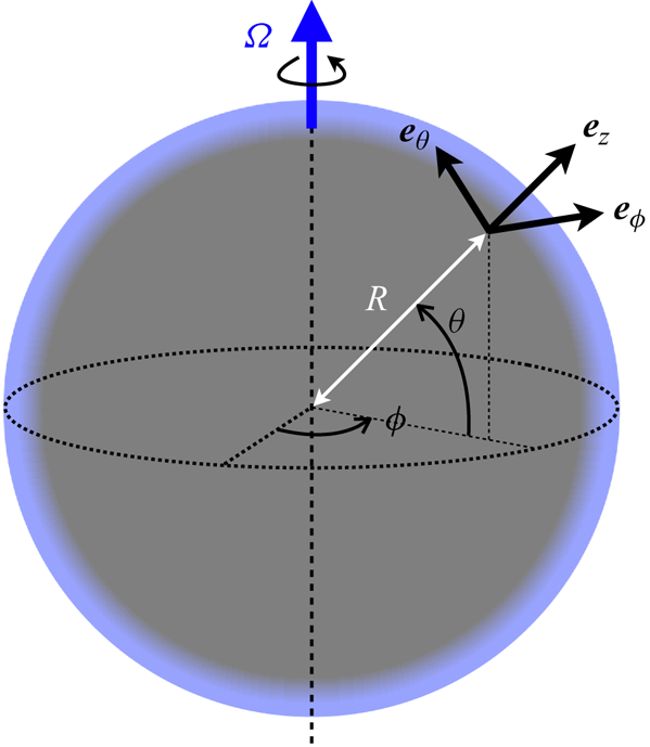
We consider the linearised shallow-water equations of an inviscid fluid layer on top of a sphere of radius $R$, rigidly rotating with constant rate $\boldsymbol {\varOmega }$ (figure 2). The fluid is initially at rest in the rotating frame. Besides, assuming that the gravity $g$ at the surface is such that $g \gg R \varOmega ^2$, we ignore centrifugal effects. Therefore, the rest state is that of a quiet layer of constant depth $h_0$. Denoting the perturbed fields with a prime, we define $\boldsymbol {v} = \boldsymbol {v}'(\boldsymbol {x},t)$ and $h = h_0 + h'(\boldsymbol {x},t)$ as the two-component velocity and height of the fluid, respectively, both functions of time $t$ and position $\boldsymbol {x}$ on the sphere. The linearised shallow-water equations can be conveniently expressed in terms of rescaled perturbation fields, i.e. $\tilde {\boldsymbol {v}} = \sqrt {h_0} \boldsymbol {v}' = \tilde {u} \boldsymbol {e}_\phi + \tilde {v} \boldsymbol {e}_\theta$ and $\tilde {h} = \sqrt {g} h'$, as

(2.1a)$$\begin{gather} \frac{\partial \tilde{\boldsymbol{v}}}{\partial t} ={-}c \boldsymbol{\nabla} \tilde{h} - \boldsymbol{f} \times\tilde{\boldsymbol{v}}, \end{gather}$$

(2.1b)$$\begin{gather}\frac{\partial \tilde{h}}{\partial t} ={-}c \boldsymbol{\nabla} \boldsymbol{\cdot} \tilde{\boldsymbol{v}}, \end{gather}$$

where $c = \sqrt {gh_0}$ is the constant phase speed and $\boldsymbol {f} = (2 \boldsymbol {\varOmega } \boldsymbol {\cdot } \boldsymbol {e}_z) \boldsymbol {e}_z$ is the projection of $2 \boldsymbol {\varOmega }$ on the local unit vector $\boldsymbol {e}_z$ normal to the surface (traditional Coriolis parameter). Since none of the parameters appearing in (2.1) depend on time or longitude, the rotating sphere acts as a waveguide trapping zonally propagating waves in the meridional direction. We can thus expand any perturbation on the set of Fourier modes $X(\theta ) \exp ({{\rm i}(m \phi - \omega t)})$, where $X$ is any of the three dependent variables of (2.1), $(\phi,\theta )$ the longitudinal and latitudinal coordinates, respectively, and $(m,\omega )$ the azimuthal wavenumber and frequency associated with the Fourier mode, which corresponds to the solutions of

(2.2a)$$\begin{gather} \omega \tilde{\boldsymbol{v}} ={-}{\rm i} c \boldsymbol{\nabla} \tilde{h} - {\rm i} \boldsymbol{f} \times \tilde{\boldsymbol{v}}, \end{gather}$$

(2.2b)$$\begin{gather}\omega \tilde{h} ={-} {\rm i} c \boldsymbol{\nabla} \boldsymbol{\cdot} \tilde{\boldsymbol{v}}. \end{gather}$$

Figure 2.

Geometry of the rotating shallow-water model on a sphere. The spherical coordinates and associated unit vectors are different from the usual ones, $\theta$ being the latitude instead of the colatitude.

The core of the discussion of this article is the metric term that arises from the divergence operator $\boldsymbol {\nabla } \boldsymbol {\cdot }$ in (2.2b), owing to the geometrical curvature of the surface. This point is discussed in § 4.

2.2. Lamb parameter and asymptotic solutions

If one rather considers the dimensionless frequency $\omega / \varOmega$, the eigenvalue problem (2.2) depends only on one dimensionless parameter:

(2.3)\begin{equation} \epsilon = \frac{c}{R \varOmega}. \end{equation}

The quantity $2/\epsilon$ is sometimes called the Lamb parameter (Müller & O'Brien Reference Müller and O'Brien1995), not to be confused with the Lamb frequency used in asteroseismology (Aerts, Christensen-Dalsgaard & Kurtz Reference Aerts, Christensen-Dalsgaard and Kurtz2010). The quantity $1/\epsilon$ gives the traversal time of a gravity wave over the spherical body in planetary days. Equations (2.2) in dimensionless units are

(2.4a)$$\begin{gather} (\omega / \varOmega) \tilde{\boldsymbol{v}} ={-}{\rm i} \epsilon \tilde{\boldsymbol{\nabla}} \tilde{h} - 2 {\rm i} \sin(\theta) \boldsymbol{e}_z \times \tilde{\boldsymbol{v}}, \end{gather}$$

(2.4b)$$\begin{gather}(\omega / \varOmega) \tilde{h} ={-} {\rm i} \epsilon \tilde{\boldsymbol{\nabla}} \boldsymbol{\cdot} \tilde{\boldsymbol{v}}, \end{gather}$$

where $\tilde {\boldsymbol {\nabla }} = R \boldsymbol {\nabla }$ is the gradient operator on the unit sphere. The parameter $\epsilon$ naturally appears in asymptotic expansions to compute the approximate spectrum of shallow-water waves (Müller & O'Brien Reference Müller and O'Brien1995; Paldor Reference Paldor2015) or their ray paths (Longuet-Higgins Reference Longuet-Higgins1965) on the sphere. One can expect to asymptotically recover the Matsuno spectrum as $\epsilon \rightarrow 0$. Indeed, expression (1.2) yields $L_{eq} / R = \sqrt {\epsilon / 2}$ for the equatorial radius of deformation, which means that, for small $\epsilon$, the wavefunctions are equatorially trapped with angular spreading of order $\sqrt {\epsilon }$, thus recovering the Cartesian $\beta$-plane approximation made by Matsuno. In this limit, the solutions of (2.2) are appropriately described with Hermite polynomials, which are exact solutions on the unbounded $\beta$-plane (see § 3.1).

Conversely, for larger values of $\epsilon$, the solutions are expected to spread away from the equator and eventually over the whole sphere. In the limit $\epsilon \gg 1$, sometimes called the Margules limit (Müller & O'Brien Reference Müller and O'Brien1995), there are two kinds of eigenvalues, originally found by Margules (Reference Margules1892) and Hough (Reference Hough1898), that we recall here:

1. (i) Those such that $\omega = {O}(c/R)$. One recovers the non-rotating shallow-water equations from (2.2). The wavefunctions are those of the Laplacian operator on a prolate spheroid, i.e. the prolate spheroidal wavefunctions (Zaqarashvili et al. Reference Zaqarashvili, Oliver and Ballester2009), and we have $R \omega / c \simeq \sqrt {\ell (\ell + 1)} - m / \epsilon$ (see e.g. Müller, Kelly & O'brien Reference Müller, Kelly and O'brien1994; Müller & O'Brien Reference Müller and O'Brien1995) with non-zero integers $\ell$ and $|m| \leq \ell$. These are global surface gravity oscillations on the sphere, perturbed by a small Coriolis term. For these solutions, the number of zeros of $\tilde {v}$ on the open interval $]-{\rm \pi} /2 , {\rm \pi}/2[$ is given by $p = \ell - |m| + 1$ (Müller & O'Brien Reference Müller and O'Brien1995).

2. (ii) Those such that $\omega = {O}(\varOmega )$. These are quasi-geostrophic planetary (Rossby) modes. From (2.2), it is straightforward to check that they obey $|\tilde {\boldsymbol {\nabla }} \boldsymbol {\cdot } \boldsymbol {v}'| = {O} ( |\boldsymbol {v}'| / \epsilon ^2 )$, i.e. that these modes have asymptotically divergence-free velocity. Eliminating the other variables from (2.2a), we end up with a second-order differential equation for $V = \cos ^\frac {3}{2} (\theta ) \tilde {v}$:

   (2.5)\begin{equation} -\frac{{\rm d}^2 V}{{\rm d} \theta^2} + \left[ \left( m^2 - \frac{1}{4}\right) \tan^2 (\theta) + \left( m^2 - \frac{1}{2} + \frac{2m \varOmega}{\omega}\right)\right] V = 0. \end{equation}

   Solutions of (2.5) are provided for instance by Taşeli (Reference Taşeli2003). They yield

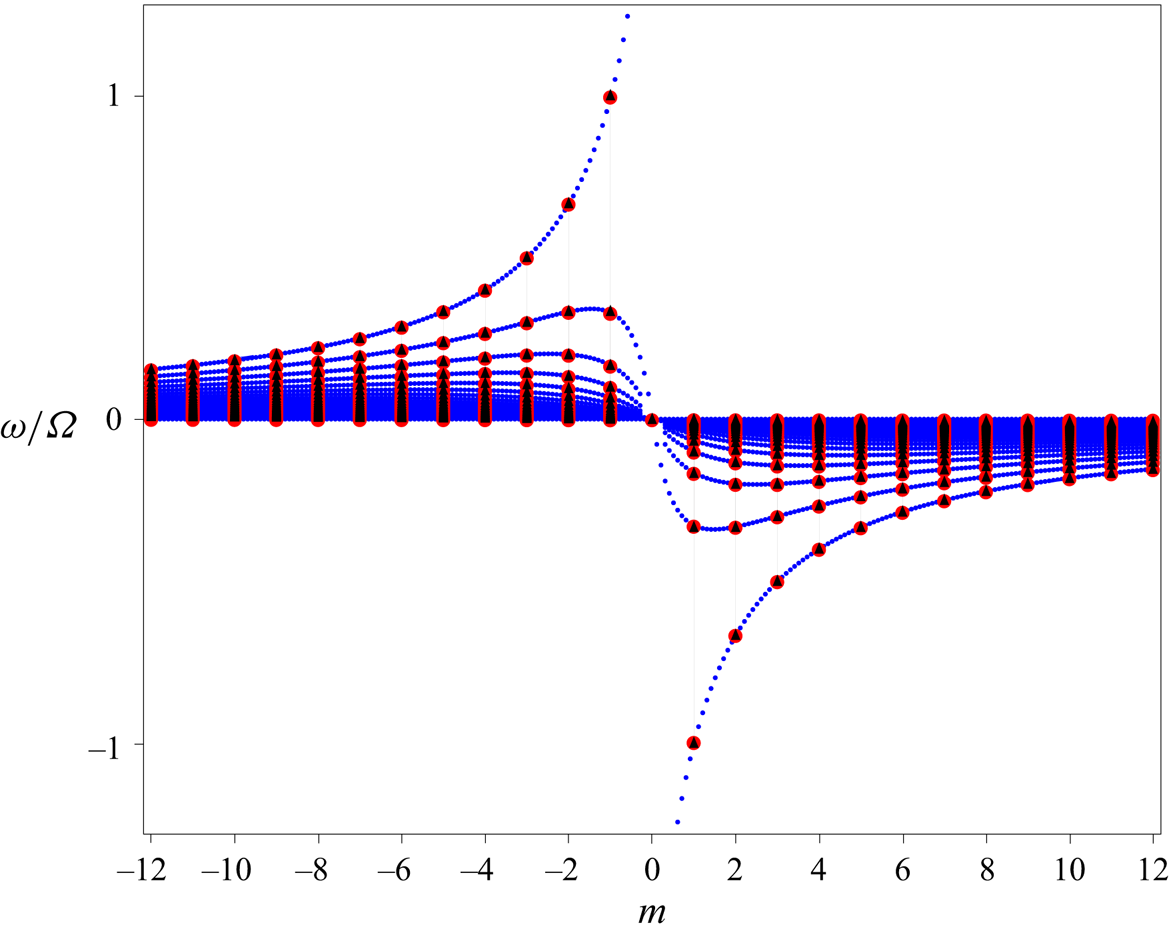
   (2.6)\begin{equation} \frac{\omega}{\varOmega} = \frac{-2m}{m^2 + (2p + 1)|m| + p(p + 1)} \quad (\text{with}\ p = 0,1,2,\dots), \end{equation}
   where the index $p$ indicates the number of zeros of the meridional velocity $\tilde {v}$ in the open interval $]-{\rm \pi} /2 , {\rm \pi}/2[$. In the Margules limit, the largest Rossby frequency is thus $\omega = \varOmega$, for $m = -1$ and $p=0$. The Rossby modes with $p=0$ constitute the westward Yanai modes (Paldor et al. Reference Paldor, Fouxon, Shamir and Garfinkel2018). Expression (2.6), which is exact for any azimuthal wavenumber $m$ in the Margules limit $\epsilon \gg 1$, is the same as (3.2c) obtained by Müller & O'Brien (Reference Müller and O'Brien1995) through a covariant formulation of the wave equations (2.1). Figure 3 provides a comparison of expression (2.6) with numerical simulations, demonstrating the convergence of the Rossby waveband towards the Margules limit as $\epsilon$ increases.

Figure 3.

Comparison between expression (2.6) (black triangles) and numerically computed Rossby frequencies for $\epsilon = 5$. The red circles are obtained by projecting (2.2) on Dedalus’ curvilinear spectral basis (Vasil et al. Reference Vasil, Lecoanet, Burns, Oishi and Brown2019), whereas the blue circles are computed from the problem (4.1) on $]-{\rm \pi} /2,{\rm \pi} /2[$, not necessarily with integer values of $m$, projecting the wavefunctions on the basis of Chebyshev polynomials (Burns et al. Reference Burns, Vasil, Oishi, Lecoanet and Brown2020) (see Appendix A). The accuracy between the numerically converged frequencies for $\epsilon =5$ and the Margules asymptotic formula (2.6) is approximately $0.4\,\%$.

There is a large frequency gap between these two wavebands, in which the Kelvin and Yanai modes of the Matsuno spectrum are absent (see figure 1).

2.3. Matsuno and Margules limits on planets and stars

As far as the shallow-water model is valid, the Matsuno regime is common to most fast-rotating planets, but also stars like brown dwarfs (Tan & Showman Reference Tan and Showman2020). Observations of the $\delta$ Scuti star Rasalhague allows one to estimate $\epsilon \simeq 0.36$ (Monnier et al. Reference Monnier, Townsend, Che, Zhao, Kallinger, Matthews and Moffat2010). Atmospheres of exoplanets cover a large range of values of $\epsilon$ (see e.g. Showman, Cho & Menou Reference Showman, Cho and Menou2010, table 1), as well as the atmosphere of Earth, for which there is a variety of values of $\epsilon$ depending on the type of waves considered (Müller & O'Brien Reference Müller and O'Brien1995; Shamir et al. Reference Shamir, Garfinkel, Gerber and Paldor2023). For instance, the measurements of Kelvin and Rossby–Haurwitz waves in the atmosphere of Venus presented by Del Genio & Rossow (Reference Del Genio and Rossow1990) lead to the estimation $\epsilon \simeq 0.9$, whereas $\epsilon \approx 70$ for the atmospheric waves considered by Showman et al. (Reference Showman, Cho and Menou2010). On Earth, equatorial Kelvin waves have been detected in both the equatorial ocean (Johnson & Mc Phaden Reference Johnson and Mc Phaden1993; Sprintall et al. Reference Sprintall, Gordon, Murtugudde and Susanto2000) and atmosphere (Kiladis et al. Reference Kiladis, Wheeler, Haertel, Straub and Roundy2009), and their implication for a variety of geophysical phenomena (e.g. the El Niño event and the Madden–Julian Oscillation) is well understood. The first baroclinic modes (the fastest ones) are such that $c \simeq 2\,{\rm m}\,{\rm s}^{-1}$ in the equatorial ocean, thus $\epsilon \simeq 4.3\times 10^{-3}$, and $c \simeq 25\,{\rm m}\,{\rm s}^{-1}$ in the atmosphere, thus $\epsilon \simeq 5.4\times 10^{-2}$ (see Vallis Reference Vallis2017, p. 304). However, the barotropic modes in the terrestrial atmosphere propagate at phase speed $c \simeq 300\,{\rm m}\,{\rm s}^{-1}$, which corresponds to $\epsilon \simeq 0.65$. This value is consistent with the data studied by Sakazaki & Hamilton (Reference Sakazaki and Hamilton2020). Surface motions on giant planets of our solar system are the subject of many recent works (Menou & Rauscher Reference Menou and Rauscher2009; Showman et al. Reference Showman, Cho and Menou2010, Reference Showman, Ingersoll, Achterberg and Kaspi2018; Gavriel & Kaspi Reference Gavriel and Kaspi2021). Atmospheric waves on Jupiter and Saturn are mostly in the Matsuno regime. For instance, eastward-propagating motions strongly localised at the equator on Jupiter have been interpreted as Kelvin waves (Legarreta et al. Reference Legarreta, Barrado-Izagirre, García-Melendo, Sanchez-Lavega and Gómez-Forrellad2016), which is consistent with the estimation $\epsilon \simeq 1.4 \times 10^{-4}$.

2.4. Opening of a spectral gap as $\epsilon$ increases

In the Margules limit ($\epsilon \gg 1$), the minimal inertia–gravity frequency is equal to $\sqrt {2} c/R$ and the maximum Rossby frequency is $\varOmega$, which yields a frequency gap of width $\varOmega (\sqrt {2} \epsilon - 1 )$ in which there is no mode. Conversely, in the Matsuno limit ($\epsilon \ll 1$), the frequency gap between Rossby and inertia–gravity modes is filled with the Yanai and Kelvin modes. However, talking about a frequency gap and branches of modes is abusive in this situation. Indeed, contrary to the zonal wavenumber $k$ of zonally propagating waves on the unbounded $\beta$-plane, the azimuthal wavenumber $m$ is not a continuous parameter, since it only takes discrete integer values. Therefore the spectrum $(m,\omega )$ does not consist of continuous branches but rather a discrete set of points, which means that, strictly speaking, there are frequency gaps between any allowed values of $\omega$. Nevertheless, the equatorial Yanai and Kelvin modes define a clear connection between the Rossby and inertia–gravity wavebands on the unbounded $\beta$-plane, which is still visible in the shallow-water spectrum on a sphere with small $\epsilon$, even if $m$ takes discrete values (see figures 1 and 4). Such a connection in the spectrum is referred to as spectral flow, which is usually defined for a continuous spectral parameter such as $k$ in unbounded flow models (Delplace et al. Reference Delplace, Marston and Venaille2017; Shankar et al. Reference Shankar, Bowick and Marchetti2017; Perrot et al. Reference Perrot, Delplace and Venaille2019; Parker et al. Reference Parker, Marston, Tobias and Zhu2020; Venaille & Delplace Reference Venaille and Delplace2021; Leclerc et al. Reference Leclerc, Laibe, Delplace, Venaille and Perez2022; Perez et al. Reference Perez, Delplace and Venaille2022; Zhu, Li & Marston Reference Zhu, Li and Marston2023). The purpose of the following section is to extend the concept of spectral flow in the present situation, i.e. with a discrete wavenumber $m$, and show that the net number of modes gained by the inertia–gravity waveband, when those modes are naturally labelled by the zeros of their meridional velocity, is actually zero for any value of $\epsilon$, even if there are transiting frequencies for small $\epsilon$ (see figure 4).

Figure 4.

Numerically computed frequencies $\omega$ for (a–f) increasing values of $\epsilon$ and $|m| \leq 20$. These converged values are obtained by projecting (2.2) on a basis of spin-weighted harmonics, a spectral method implemented in the Dedalus solver (Vasil et al. Reference Vasil, Lecoanet, Burns, Oishi and Brown2019) (see Appendix A). While for small $\epsilon$ two distinguishable spectral branches, the Yanai and Kelvin modes, transit through the gap between Rossby and gravity modes, these branches progressively break down and a clear gap opens up, separating Rossby and gravity frequencies.

3.1. Reminder: the Matsuno spectrum and wavefunctions

The shallow-water equations for equatorial waves on the unbounded $\beta$-plane are the same as (2.2), only with Cartesian coordinates instead of spherical ones ($x$ is the zonal coordinate pointing eastward and $y$ is the meridional coordinate pointing northward, with $y=0$ defining the equator), and $f=\beta y$. Once again, we focus on plane waves propagating in the zonal direction, i.e. solutions in the form $X(y) \exp ({{\rm i}(k x - \omega t)})$, where the wavenumber $k$ can take continuous values. As explained in the introduction, this model captures the physics of equatorial waves in the limit of small $\epsilon$. The solutions found by Matsuno (Reference Matsuno1966) obey the dispersion relation

(3.1)\begin{equation} \frac{\omega^2}{c^2} - k^2 - \frac{\beta k}{\omega} - \frac{\beta}{c} (2p+1) = 0 \quad (\text{with}\ p ={-}1,0,1,2,\dots), \end{equation}

and the corresponding wavefunctions for the meridional velocity are given by

(3.2)\begin{equation} \left.\begin{gathered} \tilde{v}(y) \propto H_p \left( y \sqrt{\frac{\beta}{c}} \right) \exp\left({-\frac{\beta}{2c} y^2}\right) \quad \text{for}\ p \geq 0, \\ \tilde{v}(y) = 0 \quad \text{for}\ p={-}1, \end{gathered}\right\} \end{equation}

with the Hermite polynomials $H_p$. As depicted in figure 5, the dispersion relation (3.1) can be represented by a discrete set of continuous branches in $(k,\omega )$, each indexed by the integer $p$. For $p \geq 0$, this index is equal to the number of zeros of $\tilde {v}$ in the meridional direction $y$. Branches with $p \geq 1$ are the Rossby and inertia–gravity modes. The branches $p=0$ and $p=-1$ are those of the Yanai and Kelvin modes, respectively. The Kelvin modes are purely zonal, i.e. with $\tilde {v} = 0$. The dispersion relation (3.1) formally associates Kelvin modes with the index $p=-1$ and, even though it does not make sense in terms of number of zeros of $\tilde {v}(y)$, it is convenient to keep this index $-1$ in mind. It is also worth noticing that, for $p=0$, (3.1) admits an additional solution $\omega = -ck$. This solution corresponds to a diverging mode on the unbounded $\beta$-plane, and thus it is discarded as it is not physically acceptable.

Figure 5.

The Matsuno spectrum and wavefunctions for equatorial shallow-water waves on the unbounded $\beta$-plane (Matsuno Reference Matsuno1966). (a) Plot of the dispersion relation (3.1), showing the branches $-1 \leq p \leq 3$ for positive frequencies. The Yanai and Kelvin branches transit across the frequency gap between the Rossby and inertia–gravity wavebands as $k$ increases. (b) Amplitude of the meridional velocity in the $y$ direction, given by expression (3.2). The branch index $p$ is equal to the number of zeros of $\tilde {v}(y)$.

3.2. Zeros of the meridional velocity

The $+2$ spectral flow studied by Delplace et al. (Reference Delplace, Marston and Venaille2017) corresponds to the Yanai and Kelvin modes, which transit from the Rossby waveband to the inertia–gravity waveband as $k$ increases. Beyond the fact that these modes form continuous curves in $(k,\omega )$, what identifies each of them is the number of zeros of the meridional velocity in the $y$ direction, as previously shown. Generally speaking, it is straightforward to define the spectral flow of an eigenvalue problem if there is a continuous parameter such as the zonal wavenumber $k$, because the spectrum thus consists of continuous branches. However, if the spectral parameter takes discrete values, one must find an alternative way to count the number of modes gained or lost by a waveband as this spectral parameter is swept. For shallow-water waves on a rotating sphere, the azimuthal wavenumber $m$ is a discrete parameter; nevertheless we will extrapolate the relation existing between the spectral flow of inertia–gravity waves and the number of zeros of $\tilde {v}$ for the unbounded $\beta$-plane model. In other words, we will adopt the number of zeros of $\tilde {v} (\theta )$ on the open interval $]-{\rm \pi} /2, +{\rm \pi} /2[$ as an ordering parameter for the modes of the problem (2.2) (see figure 6). In fact, many works on the spectrum of shallow-water waves associate or label modes according to the number of zeros of their meridional velocity (Hough Reference Hough1898; Longuet-Higgins Reference Longuet-Higgins1968; Iga Reference Iga1995; Müller & O'Brien Reference Müller and O'Brien1995; Paldor et al. Reference Paldor, Fouxon, Shamir and Garfinkel2018). In the Matsuno spectrum, at negative $k$, there are modes with no zero of $\tilde {v}$ in the Rossby waveband but not in the inertia–gravity waveband, whereas there are modes with no zero in the inertia–gravity waveband at positive $k$. Connecting them together forms the spectral flow of Yanai modes, which transits between the Rossby and inertia–gravity wavebands as $k$ increases. To clarify, in the rest of the paper, we employ the term modal branch to refer to modes with the same number of zeros of $\tilde {v}(\theta )$ on the open interval $]-{\rm \pi} /2, {\rm \pi}/2[$, as $m$ varies, and say that there is a modal flow when such a modal branch transits between the Rossby and inertia–gravity wavebands. In contrast, the terms spectral branch and spectral flow are used to refer to the continuous curves formed by the frequencies, which is a well-defined concept only if the spectral parameter is continuous, strictly speaking. Spectral and modal branches of the Matsuno spectrum are the same (see figure 5). In the shallow-water spectrum on the sphere, the spectral parameter $m$ is not continuous, yet one can argue that there is a spectral flow of frequencies in the Matsuno limit (see figures 1 and 4), but not in the Margules limit.

Figure 6.

(a–f) Numerically calculated frequencies of (2.2) (red circles). The modes with the same number of zeros of $\tilde {v}(\theta )$ are connected by dashed blue curves, which have no physical meaning. The number of zeros is indicated on the curves. For small $\epsilon$, the modal branches display an abrupt jump right before $m=0$. As $\epsilon$ increases, the spectrum progressively loses its east–west asymmetry and the spectral flow collapses.

As shown in the previous section, for small $\epsilon$, the ratio between the equatorial radius of deformation and the sphere's radius is of order $\sqrt {\epsilon }$, which implies that the wavefunctions spread across the whole sphere even for moderate values of $\epsilon$, and thus the modes experience the discrepancy with the unbounded $\beta$-plane. The spreading of all the wavefunctions reveals additional zeros of $\tilde {v}$ at non-zero latitude, which are virtually invisible when $\epsilon$ is too small and the modes are strongly trapped at the equator. In fact, all modes with positive phase speed (i.e. positive $m$, considering only the positive frequencies) have two additional zeros at opposite latitudes (see figures 7 and 8), compared with the same modes of the unbounded $\beta$-plane. However, the zeros of Rossby modes, which propagate westward, are unchanged. In other words, the index $p$ of the Matsuno modes propagating eastward is increased by $+2$ in spherical geometry. In particular, Yanai modes with negative $m$ have $p=0$ meridional zeros and $p=2$ zeros for positive $m$. Similarly, in contrast to the unbounded $\beta$-plane, Kelvin modes have a non-zero meridional velocity which cancels once at the equator, i.e. $p=1 = -1 + 2$. This $+2$ jump in the number of zeros, which was already discussed by Müller & O'Brien (Reference Müller and O'Brien1995), is illustrated in figure 6.

Figure 7.

Meridional velocity $\textrm {Re} (\tilde {v}(\theta ) \,\textrm {e}^{\textrm {i} m \phi } )$ of modes for $\epsilon = 0.2$ and $m=-2,+1$, computed with Dedalus (red, positive values; blue, negative values). Mode A is a Rossby mode, B and F are Yanai modes, E is a Kelvin mode and C, D, G and H are inertia–gravity modes. On the left, modes are connected by dashed blue curves according to number of zeros of $\tilde {v}(\theta )$ on $]-{\rm \pi} /2 , {\rm \pi}/2[$. Modes F, G and H have zeros at high latitude, which are not visible on the plot since the wavefunctions vanish away from the equator (see Appendix A). Dashed black lines indicate the zeros of $\tilde {v}(\theta )$, and the meridional lines of zeros correspond to the term $\textrm {e}^{\textrm {i} m \phi }$ with $m \neq 0$ for travelling waves.

Figure 8.

Same modes as figure 7, for $\epsilon = 2$. The wavefunctions are more spread in latitude and extend up to the poles, clearly revealing zeros at high latitudes. The meridional velocity of a Yanai mode has no zero for negative $m$ (B), but changes sign at two opposite latitudes for positive $m$ (F), contrary to the Yanai mode computed by Matsuno on the equatorial $\beta$-plane. Generally speaking, the meridional velocity of modes with eastward phase speed has two more zeros, compared with Matsuno's wavefunctions. Similarly, Kelvin modes (E) have zero meridional velocity on the unbounded $\beta$-plane, which is not true on the sphere. Note that the north–south symmetry of the wavefunctions is preserved on the sphere, which implies the parity of these additional zeros. This point is discussed in Appendix B.

To conclude this section, we have shown that the net modal flow of shallow-water waves, equal to $+2$ on the unbounded $\beta$-plane, is null on the sphere. This is evident for large $\epsilon$ since the spectrum displays a strong east–west symmetry, i.e. the frequencies $\omega$ and wavefunctions are nearly the same for $m$ and $-m$. As $\epsilon$ becomes smaller, the spectrum loses this east–west symmetry, displays an apparent spectral flow of frequencies but the net modal flow remains zero. At small $\epsilon$, the spectrum resembles the Matsuno one as there are Kelvin and Yanai modes transiting across the gap for increasing wavenumber $m$. However, the Yanai modes do not form a modal branch because the eastward ones have two more zeros than the westward ones. In the present case, the nullity of this modal flow can be surprising regarding the bulk–interface correspondence established by Delplace et al. (Reference Delplace, Marston and Venaille2017), Tauber, Delplace & Venaille (Reference Tauber, Delplace and Venaille2019) and Delplace (Reference Delplace2022), which states that the number of transiting modes of the Matsuno spectrum is equal to a robust topological charge $+2$ at the equator. In the following we show that the nullity of the net modal flow is actually in agreement with the index theorem, as the Chern numbers of the shallow-water spectrum on the sphere add up to zero, in contrast to the unbounded $\beta$-plane.

4.1. Hermitian form, analogy with topographic shallow-water waves

In order to apply the index theorem, we first need to express (2.2) in the form $\boldsymbol{\mathcal {H}} \boldsymbol{X} = \omega \boldsymbol{X}$, where $\boldsymbol{\mathcal {H}}$ is a Hermitian differential wave operator and the complex vector $\boldsymbol{X}$ contains the three dependent variables $\tilde {u}(\theta ),\tilde {v}(\theta )$ and $\tilde {h}(\theta )$. To do this, we introduce the rescaled fields $u = \sqrt {\cos (\theta )} \tilde {u}$, $v = \sqrt {\cos (\theta )} \tilde {v}$ and $\eta = \sqrt {\cos (\theta )} \tilde {h}$. Equation (2.2) can thus be recast in the form of a matrix eigenvalue equation:

(4.1)\begin{equation} \omega \begin{pmatrix} u \\ v \\ \eta \end{pmatrix} = \begin{pmatrix} 0 & & {\rm i} f{(\theta)} & & \dfrac{c}{R} \dfrac{m}{\cos \theta} \\ -{\rm i} f{(\theta)} & & 0 & & -{\rm i} \dfrac{c}{R} \dfrac{{\rm d}}{{\rm d} \theta} - {\rm i} \beta_{g}{(\theta)} \\ \dfrac{c}{R} \dfrac{m}{\cos \theta} & & -{\rm i} \dfrac{c}{R} \dfrac{{\rm d}}{{\rm d} \theta} + {\rm i} \beta_{g}{(\theta)} & & 0 \end{pmatrix} \begin{pmatrix} u \\ v \\ \eta \end{pmatrix} = \boldsymbol{\mathcal{H}} \begin{pmatrix} u \\ v \\ \eta \end{pmatrix}, \end{equation}

with the Coriolis parameter $f = 2 \varOmega \sin (\theta )$ and a metric $\beta$-term:

(4.2)\begin{equation} \beta_{g} = \frac{c}{2 R} \tan (\theta). \end{equation}

The problem is that of identifying the eigenvalues of the wave operator $\boldsymbol{\mathcal {H}}$, the 3-by-3 matrix of differential operators appearing in the right-hand side of (4.1). It is a Hermitian matrix operator for the canonical scalar product of complex vector functions of $\theta$ (see Appendix C). In consequence, unsurprisingly, the spectrum of shallow-water waves on the sphere is purely real. We now introduce the Weyl symbol of the wave operator $\boldsymbol{\mathcal {H}}$:

(4.3)\begin{equation} \boldsymbol{\mathsf{H}} = \begin{pmatrix} 0 & & {\rm i} f & & M \\ -{\rm i} f & & 0 & & K_\theta - {\rm i} \beta_{g} \\ M & & K_\theta + {\rm i} \beta_{g} & & 0 \end{pmatrix}, \end{equation}

where we have also defined $M = c m / (R \cos \theta )$, and $K_\theta$ the symbol of the Hermitian differential operator $-\textrm {i} \textrm {d} / \textrm {d} \theta$ times $c/R$, which is therefore a real quantity (see Hall Reference Hall2013, Theorem 13.8). Generally speaking, the symbol of a wave operator, which is obtained via the Wigner transform (see Appendix C), provides a local representation of the wave equations in phase space (see e.g. Littlejohn & Flynn Reference Littlejohn and Flynn1991; Onuki Reference Onuki2020; Perez, Delplace & Venaille Reference Perez, Delplace and Venaille2021; Venaille et al. Reference Venaille, Onuki, Perez and Leclerc2023). It extends the Fourier transform to systems of wave equations with non-constant coefficients. In the present case, the symbol $\boldsymbol{\mathsf{H}}$ represents quasi-local dispersion and polarisation relations of shallow-water waves on a sphere. Here $\boldsymbol{\mathsf{H}}$ is a continuous matrix function of the conjugated variables $\theta, K_\theta$ and $m$. To be clear, $m$ must be an integer so that the wavefunctions of $\boldsymbol{\mathcal {H}}$ are regular on the sphere, but we can formally consider the symbol $\boldsymbol{\mathsf{H}}$ as a continuous function of $m$ or $M$. In the context of this paper, we introduce it in order to apply the index theorem, following Faure (Reference Faure2023), i.e. we investigate the topological properties of the degeneracy points of $\boldsymbol{\mathsf{H}}$. This theorem relates the Chern numbers of these degeneracy points to the number and direction of transiting modes of the wave operator $\boldsymbol{\mathcal {H}}$, which can be interpreted as the spectral footprint of a degeneracy point of non-zero Chern number in the quasi-local dispersion relations. The symbol (4.3) is a generalisation of that studied by Delplace et al. (Reference Delplace, Marston and Venaille2017) for the unbounded $\beta$-plane: indeed, in the Matsuno limit, $\beta _{g} / f \approx \epsilon /4 \ll 1$ in the Yoshida waveguide, and thus the metric term $\beta _{g}$ can be dropped, as far as equatorially trapped waves are concerned.

A recent paper (Ageev & Iliasov Reference Ageev and Iliasov2024) erroneously states that the shallow-water wave operator on the sphere is non-Hermitian and admits complex eigenvalues, which is not true since this system is linearly stable in the absence of a background flow. The mistake originates from using the Fourier transform (which is not possible since the coefficients of $\boldsymbol{\mathcal {H}}$ vary with $\theta$) on the wave operator, instead of the more relevant Wigner transform. It is known that the Wigner transform must include additional terms on curved manifolds (Gneiting, Fischer & Hornberger Reference Gneiting, Fischer and Hornberger2013), which yields a Hermitian symbol in this case. Moreover, the equivalence between the respective Hermiticity of an operator and its symbol is a known property (Hall Reference Hall2013), and the symbol (4.3) is Hermitian as we used an appropriate rescaling of the variables, implying the Hermiticity of the operator $\boldsymbol{\mathcal {H}}$ for the canonical scalar product. Besides, we point out that the topological properties that are presented in the following section do not depend on the choice of $\theta$ (and thus its conjugated symbol $K_\theta$) as coordinate to express the differential operator $\boldsymbol{\mathcal {H}}$ and its symbol. Indeed, one would obtain the same symbol $\boldsymbol{\mathsf{H}}$ using any alternative coordinate $x=F(\theta )$, as long as the fields are appropriately rescaled so as to preserve the Hermiticity of $\boldsymbol{\mathcal {H}}$ (see Appendix C).

We also point out that (4.1) is formally equivalent to the shallow-water model in planar geometry with varying topography, whose transiting modes were investigated by Venaille & Delplace (Reference Venaille and Delplace2021). The metric term $\beta _{g}$ plays the exact same role as the topographic parameter $\beta _t$, although Venaille & Delplace (Reference Venaille and Delplace2021) only considered an $f$-plane. In other words, the metric $\beta$-term is mathematically analogous to topography in flat metric. Actually, one could consider together the effect of a curved metric (spherical or oblate for rapidly rotating celestial bodies, for instance) with a topography $h_0 (\theta )$ varying with latitude (thus the velocity $c=\sqrt {gh_0}$ is also a function of latitude). It can be shown that the symbol of this problem is the same as (4.3), with a total $\beta$-term that is the sum of $\beta _{g}$ and $\beta _t$. For the spherical metric with topography, this adds up to $\beta _{total} = (c/2R) ( \tan \theta - \textrm {d} \ln c / \textrm {d} \theta )$. We will not be considering a varying topography, as we focus on the curved metric. However, we bring to the analysis of Venaille & Delplace (Reference Venaille and Delplace2021) the case of varying $f$ and the additional geometric/topographic term with latitude, which was already addressed by Perez (Reference Perez2022) (part 3.5.1), in the context of the equatorial channel.

4.2. Degeneracy points of the symbol and their Chern numbers

Let us now determine the topological properties of the matrix $\boldsymbol{\mathsf{H}}$ of expression (4.3). As a function of $(m,K_\theta,\theta )$ and a 3-by-3 Hermitian matrix, $\boldsymbol{\mathsf{H}}$ has generically three eigenvalues which are real-valued functions defined over the parameter space $(m,K_\theta,\theta )$. These are referred to as eigenbands in the following, denoted $\lambda _n$ with $n=-1,0,+1$ for increasing eigenvalues. It is important to understand that these eigenvalues are not the same as the frequencies $\omega$, i.e. the eigenvalues of the operator $\boldsymbol{\mathcal {H}}$ as defined in (4.1).

The fields in (2.1) are real-valued. As such, we have $\overline {\boldsymbol{\mathcal {H}}(m)} = -\boldsymbol{\mathcal {H}}(-m)$, where the overline stands for the complex conjugation of all coefficients of $\boldsymbol{\mathcal {H}}$. Consequently, the spectrum of $\boldsymbol{\mathcal {H}}$ is completely symmetric under the inversion $(m , \omega ) \rightarrow (-m , -\omega )$. In the same way, all eigenvalues of $\boldsymbol{\mathsf{H}}$ verify

(4.4)\begin{equation} \lambda_{{-}n} (m,K_\theta,\theta) ={-}\lambda_{{+}n} ({-}m,-K_\theta,\theta), \end{equation}

for any band index $n=-1,0,+1$. Therefore, it is sufficient to consider only the positive frequencies $\omega$ of $\boldsymbol{\mathcal {H}}$, and the eigenbands $n=0$ (quasi-local representation of Rossby waves) and $n=+1$ (quasi-local representation of inertia–gravity waves) of $\boldsymbol{\mathsf{H}}$. For this reason, even though a given degeneracy point of $\boldsymbol{\mathsf{H}}$ has three Chern numbers (one for each eigenband $n=-1,0,+1$), we mostly consider the $n=+1$ one and simply refer to it as Chern number (without mentioning the band index). The characteristic polynomial of the matrix $\boldsymbol{\mathsf{H}}$ reads as

(4.5)\begin{equation} X^3 - (M^2 + K_{\theta}^2 + f^2 + \beta_{g}^2) X - 2 f \beta_{g} M. \end{equation}

The polynomial (4.5) has a multiple root, i.e. $\boldsymbol{\mathsf{H}}$ has a degenerated eigenvalue ($\lambda _{0} = \lambda _{+1}$ and/or $\lambda _{0} = \lambda _{-1}$), if and only if

(4.6)\begin{equation} \beta_{g} ={\pm} f, \end{equation}

as computed by Venaille & Delplace (Reference Venaille and Delplace2021) for the topographic shallow-water model. The degenerated positive eigenvalue ($\lambda _{0} = \lambda _{+1}$) is equal to $|f|$, and the corresponding degeneracy points in parameter space are those such that $\beta _{g} (\theta ) = \pm f (\theta )$, $M = \mp |f|$ and $K_\theta = 0$. Now the modal flow of $\boldsymbol{\mathcal {H}}$ for an eigenband $n$, i.e. the number of modes gained by the Rossby (for $n=0$) or the inertia–gravity (for $n=+1$) waveband as $m$ goes from $-\infty$ to $+\infty$, is constrained by the presence of at least one of these degeneracy points in the real system, and the value of this modal flow is given by the Chern number (a negative Chern number corresponds to a net loss of modes as $m$ increases) held by this degeneracy point for the band $n$ of the symbol (Delplace et al. Reference Delplace, Marston and Venaille2017; Perez Reference Perez2022; Faure Reference Faure2023). Since $f$ and $\beta _{g}$ have the same sign (negative in the southern hemisphere and positive in the northern one), the problem amounts to solving $c \tan (\theta ) / 2 R = 2 \varOmega \sin (\theta )$, which yields

(4.7)\begin{equation} \theta = 0 \quad \text{or} \quad \cos (\theta) = \frac{\epsilon}{4}. \end{equation}

Therefore one can distinguish two situations, as illustrated in figure 9:

1. (i) If $\epsilon < 4$, there are three latitudes at which a degeneracy between the eigenvalues of the symbol occurs, one at the equator (threefold since all three eigenvalues of $\boldsymbol{\mathsf{H}}$ are degenerated there) and two (twofold) degeneracy points near the poles, at opposite latitude. As $\epsilon$ increases, these get closer to the equator, where they eventually merge with the equatorial degeneracy point for $\epsilon = 4$. The value of $m$ at the non-equatorial degeneracy points for the positive eigenbands is

   (4.8)\begin{equation} m_c ={-}\frac{1}{2} \sqrt{1 - \left(\frac{\epsilon}{4}\right)^2} \in ]-1/2, 0[. \end{equation}

2. (ii) If $\epsilon \geq 4$, there is a unique degeneracy point at the equator. This can be seen as a threshold in the competition between two different $\beta$-effects, the traditional one owing to the variation of $f$ with latitude, which tends to trap waves at the equator, and the geometric one, which conversely tends to spread the wavefunctions away from it, over the whole sphere.

Figure 9.

Phase diagram of $\boldsymbol{\mathsf{H}}$, inspired by Haldane (Reference Haldane1988). The coloured curves represent the trajectory of $(\beta _{g}, f)$ as $\theta$ goes from $-{\rm \pi} /2$ to $+{\rm \pi} /2$. Matrix $\boldsymbol{\mathsf{H}}$ has a degenerated eigenvalue when $f = \pm \beta _{g}$ (dashed lines), thus splitting the parameter space $(\beta _{g}, f)$ into four areas, each of which is characterised by an integer $0,-1$ or $+1$. The Chern number $C_{+1}$ (coloured discs) of a degeneracy point (black circles) involving the eigenband $n=+1$ is given by their difference as $\theta$ increases past the degeneracy point. (b) If $\epsilon < 4$, the equatorial degeneracy point has $C_{+1}=+2$, the same as in Delplace et al. (Reference Delplace, Marston and Venaille2017), and there are two additional mid-latitude degeneracy points with $C_{+1}=-1$. (a) As $\epsilon$ increases and reaches $4$, they merge with the equatorial degeneracy point, which still exists for $\epsilon > 4$ and has zero Chern number. (c) The symbol of shallow-water waves on the unbounded $\beta$-plane is obtained by taking $\beta _{g} = 0$ and $f=\beta y$ in (4.3), which yields the unique degeneracy point of Chern number $+2$ studied by Delplace et al. (Reference Delplace, Marston and Venaille2017).

Each of these degeneracy points can be assigned a set of Chern numbers, one for each eigenband involved in the degeneracy (see Appendix D). Again, two situations can be distinguished:

1. (i) For $\epsilon < 4$, the equatorial threefold degeneracy point has a set of Chern numbers $(C_{-1},C_{0},C_{+1}) = (-2,0,+2)$ for the three eigenbands ($n=-1,0,+1$) of $\boldsymbol{\mathsf{H}}$, which are all degenerated. This is the result of Delplace et al. (Reference Delplace, Marston and Venaille2017) for the $\beta$-plane shallow-water model, and it still holds with the contribution of the spherical metric, as long as $\epsilon < 4$. The other twofold non-equatorial degeneracy points bear Chern numbers $(C_{0},C_{+1}) =(+1,-1)$ (for the positive-eigenband degeneracies) and $(C_{-1},C_{0}) =(+1,-1)$ (for the negative-eigenband degeneracies). Note that, for small $\epsilon$, the latter are pushed towards the poles, which are then discarded by Matsuno's $\beta$-plane approximation. This is why the $\beta$-plane shallow-water model does not have them accounted for. These negatively charged degeneracy points also appear at wavenumber $m = m_c \in ]-1/2 , 0[$, given by expression (4.8), which is why their footprint is appreciable in the form of a jump of the modal branches right before $m$ reaches $0$ (see figures 6 and 7).

2. (ii) For $\epsilon \geq 4$, all degeneracy points merge at the equator – and their respective Chern numbers add up – into a unique threefold degeneracy point which is topologically neutral, i.e. of zero Chern numbers: $(C_{-1},C_{0},C_{+1}) = (0,0,0)$. In the spectrum of the wave operator, this fusion manifests as a symmetrisation of the modes between positive and negative $m$, whereas the east–west asymmetry of the spectrum is appreciable for small $\epsilon$, when the degeneracy points are separated.

In conclusion, the metric term $\beta _{g}$ generates systematic degeneracy points whose Chern numbers compensate that of the equatorial degeneracy point. For small $\epsilon$, these degeneracy points are located near the poles and bear Chern number of $-1$ for the eigenband $n=+1$, and for $\epsilon \geq 4$ there is a unique degeneracy point at the equator whose Chern numbers are $0$. The eigenbands of $\boldsymbol{\mathsf{H}}$ thus have zero total Chern numbers, which confirms that the net number of modes gained by the inertia–gravity waveband as $m$ is swept from $-\infty$ to $+\infty$ is zero, in virtue of the index theorem. As explained in § 3, there is a direct correspondence between this mode imbalance and the evolution of the number of zeros of $\tilde {v}$ for waves on the unbounded $\beta$-plane. While the same correspondence can only be inferred by extrapolation for waves on the rotating sphere, we showed here that the absence of modal flow is in agreement with the predictions of topology. For the unbounded $\beta$-plane, Venaille et al. (Reference Venaille, Onuki, Perez and Leclerc2023) provide a formal proof of the equality between the modal flow (i.e. the difference in number of positive-frequency inertia–gravity modes between the two limits $k \rightarrow + \infty$ and $k \rightarrow -\infty$) and the Chern number of the symbol's degeneracy point at the equator, based on geometric Wentzel–Kramers–Brillouin analysis of the waves in both limits. This study, which provides an alternative point of view to the index theorem, could also be extended here to demonstrate the nullity of this mode imbalance on a sphere, with the wavenumber $m$ instead of $k$.

4.3. Collapse of the spectral flow

For $\epsilon < 4$, one could expect that each of the degeneracy points exhibited in § 4.2 should be associated with its own branch of modes, two of them localised near the equator, transiting from the Rossby waveband to the inertia–gravity waveband as $m$ increases (corresponding to the $+2$ topological charge at the equator), and two localised near the latitudes $\pm \theta$ such that $\cos \theta = \epsilon / 4$, transiting from the inertia–gravity waveband to the Rossby waveband as $m$ increases (corresponding to the $-1$ charges). However, there is no footprint of the modes transiting from the inertia–gravity waveband to the Rossby waveband, and this happens for two reasons:

1. (i) Although the index theorem applies individually for each degeneracy point of the symbol, the resulting spectral flows are visible only in a semi-classical limit (Faure Reference Faure2023), i.e. as long as the transiting modes are well separated in phase space (Jezequel & Delplace Reference Jezequel and Delplace2023). In the case of shallow-water waves on a rotating sphere, the semi-classical limit in question corresponds to $\epsilon \ll 1$. Indeed, the equatorial waves spread up to the poles even for moderate values of $\epsilon$ ($\epsilon \sim 1$), which means that the modes corresponding to the opposite spectral flows overlap and hybridise, thus manifesting an avoided crossing between their respective spectral branches (see e.g. the cases studied by Kaufman et al. (Reference Kaufman, Morehead, Brizard and Tracy1999) and Perez (Reference Perez2022), part 3.5.1), which is precisely why the spectral flow of frequencies collapses as $\epsilon$ increases.

2. (ii) Even for $\epsilon \ll 1$ the modes of negative spectral flow are not visible in the spectrum. We showed in § 4.2 that these are expected to be localised near the poles, as are the corresponding degeneracy points of the symbol, and transit around $m \approx -1/2$. These modes are the spherical counterpart of Matsuno's spurious solutions (for $\omega = -c k$), or coastal Kelvin waves in the equatorial channel (Paldor Reference Paldor2015; Venaille & Delplace Reference Venaille and Delplace2021; Perez Reference Perez2022), if the edges of the channel were moved up to the poles. Owing to the spherical geometry, the dispersion relation of coastal Kelvin modes propagating along a longitudinal wall at latitude $\theta$ is $\omega = -cm/R \cos \theta$. Therefore, the slope of the branches formed by these hypothetical polar modes is large, and they do not appear in the spectrum for integer values of the wavenumber $m$ since they transit around $m \approx -1/2$. For small $\epsilon$, the strong east–west asymmetry is the manifestation of these opposite topological charges being separated, the gap-crossing Kelvin and Yanai frequencies are the footprint of the $+2$ topological charge at the equator, while the abrupt $+2$ modal jump happening between $m=-1$ and $m=0$ (see figure 6) is the footprint of the degeneracy points of charges $-1$ located near the poles.