2 The modified Townsend–Perry model

The modified model proposed by Vassilicos et al. (Reference Vassilicos, Laval, Foucaut and Stanislas2015) for the energy spectrum $E_{11}(k_{1},y)$ in the region $\unicode[STIX]{x1D708}/u_{\unicode[STIX]{x1D70F}}\ll y\ll \unicode[STIX]{x1D6FF}$ is defined in four wavenumber ranges ( $\unicode[STIX]{x1D708}$ being the kinematic viscosity). The Kolmogorov range $1/y<k_{1}$ is identical to the Townsend–Perry model following the form $E_{11}(k_{1},y)\sim \unicode[STIX]{x1D716}^{2/3}k_{1}^{-5/3}g_{K}(k_{1}y,k_{1}\unicode[STIX]{x1D702})$ . However, what is referred to as the ‘attached-eddy’ range where $E_{11}(k_{1})\approx C_{0}u_{\unicode[STIX]{x1D70F}}^{2}k_{1}^{-1}$ in the Townsend–Perry model is restricted to the range $1/\unicode[STIX]{x1D6FF}_{\ast }<k_{1}<1/y$ (instead of the Townsend–Perry model’s original range $1/\unicode[STIX]{x1D6FF}<k_{1}<1/y$ ) and a new scaling $E_{11}(k_{1})\approx C_{1}u_{\unicode[STIX]{x1D70F}}^{2}\unicode[STIX]{x1D6FF}(k_{1}\unicode[STIX]{x1D6FF})^{-m}$ with $0<m<1$ is proposed in the range $1/\unicode[STIX]{x1D6FF}_{\infty }<k_{1}<1/\unicode[STIX]{x1D6FF}_{\ast }$ where $\unicode[STIX]{x1D6FF}_{\ast }$ and $\unicode[STIX]{x1D6FF}_{\infty }$ are two large length scales such that $\unicode[STIX]{x1D6FF}_{\ast }\leqslant \unicode[STIX]{x1D6FF}_{\infty }$ . The spectra at very large scales $k_{1}<1/\unicode[STIX]{x1D6FF}_{\infty }$ are kinematically constrained to be independent of $k_{1}$ and therefore of the form $E_{11}(k_{1})\approx C_{\infty }u_{\unicode[STIX]{x1D70F}}^{2}\unicode[STIX]{x1D6FF}$ . This new model predicts that the new range $1/\unicode[STIX]{x1D6FF}_{\infty }<k_{1}<1/\unicode[STIX]{x1D6FF}_{\ast }$ where $E_{11}(k_{1})\approx (k_{1}\unicode[STIX]{x1D6FF})^{-m}$ is present only for $y$ smaller than a wall distance $y_{\ast }$ above which the original Townsend–Perry model is valid without alterations.

By integration of $E_{11}(k_{1})$ we obtain the modified model for the mean square streamwise fluctuating velocity in the range $\unicode[STIX]{x1D708}/u_{\unicode[STIX]{x1D70F}}\ll y\leqslant y_{\ast }=\unicode[STIX]{x1D6FF}A^{1/p}Re_{\unicode[STIX]{x1D70F}}^{-q/p}$ :

with

and where $\unicode[STIX]{x1D6FC}$ , $B$ , $p$ and $q$ are the parameters used in the power-law formulation of the two scales $\unicode[STIX]{x1D6FF}_{\ast }$ and $\unicode[STIX]{x1D6FF}_{\infty }$ as a function of wall distance and Reynolds number:

and

where $\unicode[STIX]{x1D6FD}=\unicode[STIX]{x1D6FC}\,q/p$ and $B=A^{-\unicode[STIX]{x1D6FC}/p}$ . This model predicts that the location $y_{peak}$ of the outer peak or plateau scales as $\unicode[STIX]{x1D6FF}\,Re_{\unicode[STIX]{x1D70F}}^{-q/p}$ , i.e. $y_{peak}^{+}\sim Re_{\unicode[STIX]{x1D70F}}^{1-q/p}$ . In the region where $y_{\ast }<y$ , (1.1) holds and completes the model.

The parameters of this new model (2.1)–(2.4) have been evaluated against the Princeton superpipe energy spectra for a large-Reynolds-number range ( $1985<Re_{\unicode[STIX]{x1D70F}}<98\,160$ ) by Vassilicos et al. (Reference Vassilicos, Laval, Foucaut and Stanislas2015). It was shown that the new model is able to reproduce the correct scaling of the outer peak with a single set of parameters for all Reynolds numbers. It is important to determine whether this new model can also account for a variety of high-Reynolds-number turbulence boundary layer data and whether it can do it without much variation in its defining parameters.

3 Fits of high-Reynolds-number turbulent boundary layer data

In order to test the universality of the model (1.1), (2.1)–(2.4), statistics from several large-Reynolds-number turbulent boundary layer experiments have been collected. As already shown by Hultmark et al. (Reference Hultmark, Vallikivi, Bailey and Smits2012), the mean square streamwise fluctuating velocity exhibits a clear outer peak for extremely large Reynolds number only. As very few experimental results are available for $Re_{\unicode[STIX]{x1D70F}}>40\,000$ and as the model is designed and able to capture the outer peak or plateau region even in the absence of a clear peak, the model is also fitted here on data from experiments with smaller Reynolds numbers where the statistics of $\overline{u^{\prime 2}}$ do not display an outer peak but just a tendency towards a plateau. The minimum Reynolds number required to fit the parameters of the model should be such that there is at least a short range of wall distances where the log decay of $\overline{u^{\prime 2}}$ is visible. In the present contribution, data sets from four turbulent boundary layer experiments are investigated and compared, covering a range of Reynolds numbers from $Re_{\unicode[STIX]{x1D70F}}\simeq 3200$ to $Re_{\unicode[STIX]{x1D70F}}\simeq 72\,000$ . The models parameters are also compared with the original values from the fits of the Princeton superpipe data by Vassilicos et al. (Reference Vassilicos, Laval, Foucaut and Stanislas2015).

The first set of data has been recorded in the turbulent boundary layer wind tunnel of Lille, which has a test section length of 20.6 m in the streamwise direction ( $x$ -direction) and a cross-section 2 m wide and 1 m high. Four free-stream velocities were investigated from $U=3~\text{m}~\text{s}^{-1}$ to $U=10~\text{m}~\text{s}^{-1}$ leading to a Reynolds number range from $Re_{\unicode[STIX]{x1D70F}}=3200$ to $Re_{\unicode[STIX]{x1D70F}}=7000$ . The statistics are detailed in Carlier & Stanislas (Reference Carlier and Stanislas2005). The hot-wire data were recorded at 19.6 m from the entrance of the test section and the friction velocities were measured using macro-PIV by Foucaut, Kostas & Stanislas (Reference Foucaut, Kostas and Stanislas2006). The second set of data is from hot-wire measurements in the large boundary layer wind tunnel at University of Melbourne. It has a 27 m long test section of $2\times 2~\text{m}^{2}$ . The statistics of the two lower Reynolds numbers are presented in Marusic et al. (Reference Marusic, Chauhan, Kulandaivelu and Hutchins2015) whereas the data for $Re_{\unicode[STIX]{x1D70F}}=19\,000$ were extracted from Marusic, Mathis & Hutchins (Reference Marusic, Mathis and Hutchins2010). The third set of data is from the turbulent boundary layer flow physics facility (FPF) at the University of New Hampshire (UNH), which is able to reach similar Reynolds numbers with a much longer test section (72 m) and a lower free-stream velocity ( $U=13.75~\text{m}~\text{s}^{-1}$ ). The facility and the hot-wire data are described in Vincenti et al. (Reference Vincenti, Klewicki, Morrill-Winter, White and Wosnik2013). The facility is an open circuit suction tunnel that draws from, and discharges to, the atmosphere. The streamwise free-stream turbulence intensity for $U>7~\text{m}~\text{s}^{-1}$ is less than approximately 0.3 %. The fourth and last set of data investigated here are the turbulent boundary layer and the turbulent pipe data from the Princeton superpipe (see Vallikivi et al. Reference Vallikivi, Hultmark and Smits2015). A comparison of spectra from both superpipe experiments over the same range of Reynolds numbers ( $3000<Re_{\unicode[STIX]{x1D70F}}<70\,000$ ) was conducted by Vallikivi, Ganapathissubramani & Smits (Reference Vallikivi, Ganapathissubramani and Smits2014) leading to five scaling regions for the turbulent pipe and the turbulent boundary layer. The data acquired with the Nano Scale Thermal Anemometry Probe (NSTAP) are known to be affected by insufficient probe resolution (see table 1). As in most studies of the authors of the NSTAP data, the present analysis is conducted with the data corrected for spatial filtering (see Smits et al. Reference Smits, Monty, Hultmark, Bailey, Hutchins and Marusic2011). The correction affects mainly the statistics of the two highest Reynolds numbers ( $Re_{\unicode[STIX]{x1D70F}}>40\,000$ ) for $y^{+}<300$ . However, the present analysis was also conducted on the raw data to check that the quantitative conclusions of the present paper do not change significantly.

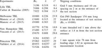
The data of each experiment are affected by different statistical convergence levels and/or slightly different experimental conditions. Some important characteristics of the four TBL experiments are summarised in table 1. For instance, the LML facility produces a slight favourable pressure gradient ( $-0.5~\text{Pa}~\text{m}^{-1}$ at $10~\text{m}~\text{s}^{-1}$ ), which is not the case for the New Hampshire and the Melbourne facilities. Hot-wire acquisition times are of the order of 12 000 $U_{\infty }/\unicode[STIX]{x1D6FF}$ for the Melbourne and LML facilities and two to four times smaller for the New Hampshire facility, depending on the Reynolds number. This can explain apparent different levels of convergence of some statistics. There are also different tripping conditions for the TBL experiments with respect to the size of the boundary layer thickness (see table 1) and in the way that scaling parameters such as friction velocity ( $u_{\unicode[STIX]{x1D70F}}$ ) and boundary layer thickness ( $\unicode[STIX]{x1D6FF}$ ) have been determined by different techniques. For instance, the boundary layer thickness is determined as $\unicode[STIX]{x1D6FF}_{99}$ , except for the Melbourne data, where $\unicode[STIX]{x1D6FF}$ is determined from a modified Coles law of the wall/wake fit to the mean velocity profile. This method can overestimate $\unicode[STIX]{x1D6FF}$ by up to 25 % with respect to $\unicode[STIX]{x1D6FF}_{99}$ , depending on the Reynolds number. The friction velocity $u_{\unicode[STIX]{x1D70F}}$ is either determined by Preston tube or Clauser plot. The accuracy of both methods is known to be of the order of a few percent. The values of $u_{\unicode[STIX]{x1D70F}}$ for the Lille experiments are validated by micro-PIV.

Figure 1.

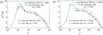
Comparison of $\overline{u^{\prime 2}}/u_{\unicode[STIX]{x1D70F}}^{2}$ versus $y^{+}$ for several turbulent boundary layer and pipe flow experiments at two Reynolds numbers: (a)  $Re_{\unicode[STIX]{x1D70F}}\simeq 7000$ , (b)  $Re_{\unicode[STIX]{x1D70F}}\simeq 20\,000$ .

Table 1.

Parameters of the four turbulent boundary layer experiments. The boundary layer thickness $\unicode[STIX]{x1D6FF}$ corresponds to $\unicode[STIX]{x1D6FF}_{99}$ except for Melbourne TBL, where $\unicode[STIX]{x1D6FF}$ is determined from a modified Coles law of the wall/wake fit to the mean velocity profile; $\ell ^{+}$ is the sensor length in wall units.

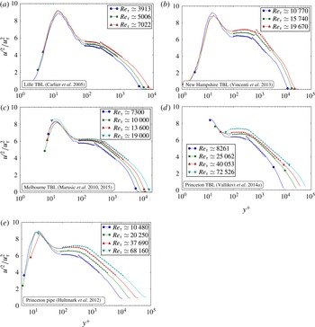
In figure 1 we plot, for comparison, mean square streamwise fluctuating velocity profiles from different experiments at two similar Reynolds numbers. As both the boundary layer thickness and the length of the hot wires are different, the comparison of the results in the region of the first peak ( $y^{+}<30$ ) is not significant, especially at the highest Reynolds number. Due to a different definition of the boundary layer thickness, the Reynolds number for the Melbourne data may be overestimated, which may explain the slightly lower values of mean square streamwise fluctuating velocity profiles. However, taking into account the slightly different Reynolds number values and experimental conditions in each plot of figure 1, and the uncertainty in the friction velocity evaluations, it can be said that the four experiments exhibit comparable overall behaviours. The values of $\overline{u^{\prime 2}}$ in the New Hampshire TBL are, however, slightly higher than the average of the three other experiments for the higher of the two Reynolds numbers (figure 1 b). The log decay (1.1) is clearly defined only at the highest Reynolds number ( $Re_{\unicode[STIX]{x1D70F}}\simeq 20\,000$ ), except for the New Hampshire TBL data, for which the outer peak is more pronounced and extends to higher  $y^{+}$ .

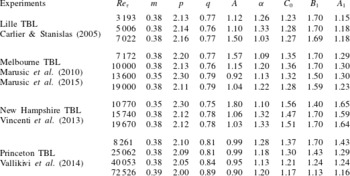
As a first test, the model (1.1), (2.1)–(2.4) was fitted to each Reynolds number data of each dataset independently. This results in a set of optimal parameters defined in table 2. The two regions $y<y_{\ast }$ and $y>y_{\ast }$ are fitted at the same time, but as the parameters $A_{1}$ and $B_{1}$ involved in the log-decay region $y>y_{\ast }$ are fitted independently of $C_{0}$ , the two fitted parts do not perfectly match. The extent of the region with the logarithmic decay (1.1) is not a priori certain. In the present case, a conservative but widely accepted upper bound $y<0.15\unicode[STIX]{x1D6FF}$ was used. This choice leads to a rather short logarithmic region for the lower Reynolds numbers investigated here, and consequently a substantial uncertainty in the determination of the two constants $B_{1}$ and $A_{1}$ . The two parts of the model, as well as the wall distance $y_{\ast }$ where the two models merge, are fitted simultaneously using a L-BFGS-B algorithm developed by Byrd, Lu & Nocedal (Reference Byrd, Lu and Nocedal1995) for the solution of the optimisation problem.

Table 2.

Best values of the model parameters (1.1), (2.1)–(2.4) for the fit of the four turbulent boundary layer datasets.

The first conclusion is that the model is able to fit the complete dataset with parameter values which do not vary significantly with Reynolds number and from one experiment to the other. The two exponents $p$ and $q$ control the wall distance of the outer peak or plateau as well as the related Reynolds number and wall-distance dependencies of the new spectral range extent $\unicode[STIX]{x1D6FF}_{\infty }/\unicode[STIX]{x1D6FF}_{\ast }$ . The values obtained for $p$ and $q$ appear relatively constant across Reynolds numbers and across TBL experiments. They appear also fairly close to those obtained by Vassilicos et al. (Reference Vassilicos, Laval, Foucaut and Stanislas2015) for the Princeton high-Reynolds-number turbulent pipe flow. These values of $q$ and $p$ suggest an outer peak position scaling like $y_{peak}^{+}\sim Re_{\unicode[STIX]{x1D70F}}^{2/3}$ (following § 2, $1-q/p\simeq 0.61$ , which is close to  $2/3$ ), and the fact that $\unicode[STIX]{x1D6FC}$ is always larger than 1 suggests that an outer peak does indeed exist (see Vassilicos et al. (Reference Vassilicos, Laval, Foucaut and Stanislas2015) for an explanation of this point). However, the ratio $q/p$ seems to decrease slightly for the Princeton TBL with increasing Reynolds number. The parameter $m$ which, in the model, controls the slope of the $k_{1}^{-m}$ spectrum in the new range $1/\unicode[STIX]{x1D6FF}_{\infty }<k_{1}<1\unicode[STIX]{x1D6FF}_{\ast }$ is extremely stable as compared, for instance, to  $\unicode[STIX]{x1D6FC}$ . However, the two values appear to be correlated so that a small variation of the former can be compensated by the latter. The parameter $C_{0}$ which controls the amplitude of the outer peak does not vary too much and remains close to a mean value of 1.33. The larger values of $C_{0}$ for the New Hampshire data are linked to the more pronounced outer peak as already noticed in figure 1. The parameters $A_{1}$ and $B_{1}$ of the log-decay model (1.1) are only significant at the highest Reynolds numbers investigated, where this log-decay region is clearly defined. They are also dependent on the lower bound on $y$ chosen to fit the model (1.1). In our model, the log-decay region starts at the wall distance $y_{\ast }$ which was used to fit the two parameters $A_{1}$ and $B_{1}$ . The average values of these two parameters, keeping only the seven cases with $Re_{\unicode[STIX]{x1D70F}}>12\,000$ , are $A_{1}\simeq 1.35$ and $B_{1}\simeq 1.45$ . The average slope $A1$ is close to the value reported by Marusic et al. (Reference Marusic, Monty, Hultmark and Smits2013) with a different definition of the fitting lower bound and taking into account their 95 % confidence estimated error bars.

Table 3.

Best values of the model parameters (1.1), (2.1)–(2.4) for the fit of the four turbulent boundary layer datasets and the Princeton superpipe data. The fit was performed by fixing four of the parameters ( $m=0.38$ , $p=2.1$ , $A=1.0$ and $\unicode[STIX]{x1D6FC}=1.2$ ).

Figure 2.

Fit of each experiment dataset with the model (1.1), (2.1)–(2.4) using four variable parameters ( $q$ , $C_{0}$ , $B_{1}$ , $A_{1}$ ) and the remaining ones fixed at $m=0.38$ , $p=2.1$ , $A=1.0$ and $\unicode[STIX]{x1D6FC}=1.2$ .

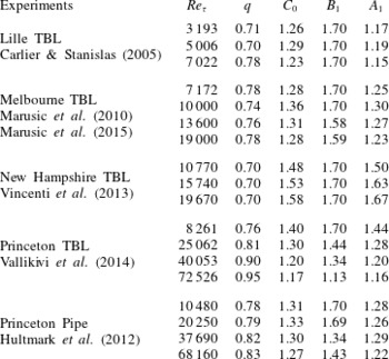
As a second test of robustness of the model, the data of the four TBL experiments were fitted with the model whilst keeping a constant value for four parameters ( $m=0.38$ , $p=2.1$ , $A=1.0$ and $\unicode[STIX]{x1D6FC}=1.2$ ). The values of these four parameters are taken as the approximate average of the first estimation when all parameters are fitted. We choose to adjust the four remaining parameters $q$ , $C_{0}$ , $B_{1}$ and $A_{1}$ for two reasons. Firstly, the model is sensitive to the ratio $p/q$ which controls the location of the outer peak and more importantly the wall distance $y_{\ast }$ associated with the merging of the two parts of the model. Secondly, the other three parameters $C_{0}$ , $B_{1}$ and $A_{1}$ are associated with the amplitude of the outer peak and the slope and level of the log-decay region. The values of $A_{1}$ and $B_{1}$ in (1.1) vary from one experiment to the other in particular because this region is well established only at extremely large Reynolds numbers but also because there is no clear consensus on the exact bounds on $y$ where this log-decay region exists. The four fitted parameters are given in table 3 and the resulting fits for the four TBL data (and for the Princeton turbulent pipe data for comparison) are shown in figure 2. The first part of the model (i.e. (2.1)–(2.4) for $80\unicode[STIX]{x1D708}/u_{\unicode[STIX]{x1D70F}}\lesssim y<y_{\ast }$ ) which results from the addition of the new spectral range $1/\unicode[STIX]{x1D6FF}_{\infty }<k_{1}<1/\unicode[STIX]{x1D6FF}_{\ast }$ is able to return good fits for all the experiments and all the Reynolds numbers investigated. The parameters $C_{0}$ and $q$ which control the amplitude and location of the outer peak (or plateau for $7000<Re_{\unicode[STIX]{x1D70F}}<20\,000$ ) take values similar to the previous fit (table 2); the root-mean-square (r.m.s.) difference on these two parameters is only approximately 3 % between tables 2 and 3. The variations in the values of the log-decay parameters $B_{1}$ and $A_{1}$ with respect to table 2 are due to the slight changes of the lower bound $y_{\ast }$ . Finally, the parameters $q$ , $C_{0}$ , $A_{1}$ and $B_{1}$ are also given for the Princeton turbulent pipe data at four Reynolds numbers. At similar Reynolds numbers, the differences in the values of these four parameters between the two types of flow (TBL and turbulent pipe flow) are comparable to the differences in their values from one TBL experiment to the other.

Figure 3.

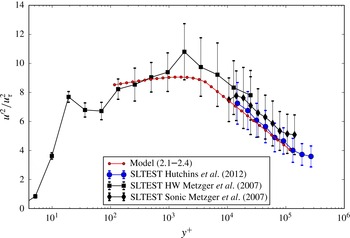
Comparison of $\overline{u^{\prime 2}}/u_{\unicode[STIX]{x1D70F}}^{2}$ for the measurements campaign of the SLTEST experiments with the model (1.1)–(2.1)–(2.3) using the averaged parameters obtained from previous fit for the highest Reynolds numbers ( $m=0.38$ , $p=2.1$ , $q=0.81$ , $A=1.0$ , $\unicode[STIX]{x1D6FC}=1.21$ , $C_{0}=1.4$ , $B_{1}=1.4$ , $A_{1}=1.4$ ). The Reynolds numbers based on boundary layer thickness were estimated as $60\times 10^{6}$ and $80\times 10^{6}$ for the Metzger, McKeon & Holmes (Reference Metzger, Mckeon and Holmes2007) and Hutchins et al. (Reference Hutchins, Kapil, Marusic, Monty and Klewicki2012) data respectively, corresponding to $Re_{\unicode[STIX]{x1D70F}}\simeq 770\,000$ and $Re_{\unicode[STIX]{x1D70F}}\simeq 780\,000$ , respectively.

The evidence obtained from the present analysis points to a wide applicability of the model (2.1)–(2.4) and (1.1), with parameter values which do not vary much from one flow to the other (a wide range of Reynolds numbers $Re_{\unicode[STIX]{x1D70F}}$ from 7000–70 000, two types of wall-bounded turbulent flows and four different installations). This motivates us to propose a best set of values for all eight parameters of the model which can be used for predictive purposes, for example when extrapolating to near-wall turbulence at even higher Reynolds numbers. However, very few data are available to test such extrapolation. An example of such rare data was obtained from highly documented measurements performed at SLTEST, an atmospheric facility in the Great Salt Lake Desert. Several sets of experiments were conducted in this facility, but we focus only on the most reliable ones, the sonic anemometer data from Hutchins et al. (Reference Hutchins, Kapil, Marusic, Monty and Klewicki2012) and the hot-wire and sonic anemometer data from Metzger et al. (Reference Metzger, Mckeon and Holmes2007). The first set covers only part of the log-decay region while both hot-wire and sonic anemometer data are available from the second set covering the two specific regions of the present model. As parameters vary a little with Reynolds number when the Reynolds number is not high enough, the parameters used for the extrapolation were computed as their average for TBL with $Re_{\unicode[STIX]{x1D70F}}\geqslant 12\,000$ (table 2) only. This leads to $A_{1}\simeq 1.35$ , $B_{1}\simeq 1.45$ , $A\simeq 1.0$ , $\unicode[STIX]{x1D6FC}\simeq 1.21$ , $p\simeq 2.1$ , $q\simeq 0.81$ , $m\simeq 0.38$ and $C_{0}\simeq 1.32$ . However, as the continuity of the model at $y=y_{\ast }$ imposes $A_{1}=B_{1}=C_{0}$ (see Vassilicos et al. (Reference Vassilicos, Laval, Foucaut and Stanislas2015) for full explanations) we choose a compromise value of $A_{1}=B_{1}=C_{0}=1.4$ , keeping the other parameters to their average value.

These average values for $p$ , $m$ , $\unicode[STIX]{x1D6FC}$ and $A$ are also the values chosen for our second fit (table 3). The two sets of SLTEST data as well as our model parameters and prediction are shown in figure 3. The values chosen for $A_{1}$ and $B_{1}$ lead to a prediction of the log-decay region in general agreement with the two sets of data, taking into account the error bars proposed by the authors. The model predicts an outer peak in global agreement with the hot-wire data of Metzger et al. (Reference Metzger, Mckeon and Holmes2007), given the accuracy of the experimental results. In fact, the outer peak returned by the model looks more like a plateau with a weak slope. Putting aside the point of Metzger et al. at $y^{+}=2000$ which is potentially questionable, the global shape and level predicted by the extrapolation of our model to these extremely high Reynolds numbers agrees reasonably well with the SLTEST data down to $y^{+}=150$ . It would be of interest to have more reliable measurements of the inner peak in such a flow to see how the inner and outer peaks connect.