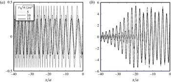
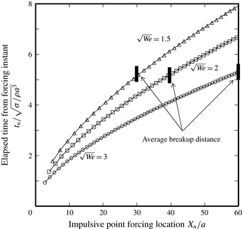
1 Introduction
Convective instability plays a major role in various types of flows of engineering interest, and it is thus important to understand its origin in depth. For example, direct numerical simulation (DNS) is now often used to simulate a complex flow field. Any DNS is associated with numerical errors. A DNS of a jet flow can be validated only if it correctly captures the origin of the involved convective instability in the physical formulation of the problem. The use of a grid-independence test is common practice in checking that the calculated convective instability is not triggered by numerical errors (noise). In other words, we expect that the convective instability calculated by the DNS is excited in a deterministic way by the dynamic system on which the DNS is based. However, there is no established theory supporting this expectation. Therefore, exploring the origins of various convective instabilities is necessary for designing an appropriate DNS, as well as for quantitatively predicting instability results of engineering interest. In this respect, the Plateau (Reference Plateau1873) and Rayleigh (Reference Rayleigh1878) (hereafter abbreviated as PR) unstable wave is considered to serve as a good prototype for gaining general insights into the origin of convective instability.
A low-speed water jet issued from an orifice into still air spontaneously disintegrates into droplets by either end-pinching (nonlinear instability) (Batchelor Reference Batchelor1958; Taylor Reference Taylor1959; Stone & Leal Reference Stone and Leal1989; Schulkes Reference Schulkes1996; Umemura Reference Umemura2011) or the growth of the PR unstable wave (convective instability). The energy source of both instabilities is surface energy release. Which disintegration mode dominantly operates depends on the jet-issue speed. Water issued downwards under normal gravity exhibits dripping at small jet-issue speeds, where end-pinching is dominant. In a jetting state at large jet-issue speeds, the PR unstable wave growth governs the jet disintegration. In between, transitional behaviours between dripping and jetting are observable (Clanet & Lasheras Reference Clanet and Lasheras1999; Ambravaneswaran et al. Reference Ambravaneswaran, Subramani, Phillops and Basaran2004). End-pinching is a local nonlinear instability inherent to a liquid jet tip, and tends to occur whenever a new liquid jet tip is created. On the other hand, the convective instability can operate only when the initial PR unstable wave elements are somehow produced upstream.
In the present study, we assume that any PR unstable wave has a small initial magnitude of amplitude. The jet surface appears smooth near the injector and disintegrates somewhere downstream. One of the main purposes of the linear stability analysis is to find a mode of maximum growth rate as the most unstable mode for the jet. This is because, irrespective of the initial perturbations, the most unstable mode will eventually become dominant and the jet disintegration is considered to be caused by the most unstable mode. When a circular (radius
 $a_{\ast }$
) liquid column initially at rest in still gas is subjected to a small sinusoidal surface deformation with a wavelength
 ${\it\lambda}_{\ast }>2{\rm\pi}a_{\ast }$
, it exhibits a temporally growing surface deformation amplitude (Plateau Reference Plateau1873). The maximum temporal growth rate,
 ${\it\varpi}_{\ast }$
, is attained for
 ${\it\lambda}_{\ast }\cong 9a_{\ast }$
, and results in the shortest breakup time,
 $t_{B\ast }={\it\varpi}_{\ast }^{-1}\ln (a_{\ast }/{\it\varepsilon}_{\ast })$
, for an initial surface deformation amplitude,
 ${\it\varepsilon}_{\ast }$
. If this deformed liquid column is produced at the orifice exit and moves with the jet speed,
 $U_{\ast }$
, experiencing the same temporal evolution as mentioned above, the breakup length of the jet is predicted to be
 $L_{B\ast }=U_{\ast }t_{B\ast }$
. This is an important result derived from Rayleigh’s theory. A more accurate approach to this problem can be made in spatial evolution analyses. Keller, Ubinow & Tu (Reference Keller, Ubinow and Tu1973) conducted a spatial linear stability analysis and showed that the same PR unstable wave as that predicted from a temporal linear stability analysis emerges in the limit of an infinitely large jet-issue speed. Therefore, the jet-issue speed is also an important parameter characterising the most unstable mode. Based on a spatiotemporal linear stability analysis, Leib & Goldstein (Reference Leib and Goldstein1986) predicted that an orifice jet exhibits absolute instability (Landau Reference Landau1949) or convective instability, depending on the jet-issue speed.
In the 1970s, extensive analyses were conducted to control the jet-disintegration state. In this problem, a PR unstable wave is periodically produced by a sinusoidal change in the jet-issue speed about a prescribed value. Using linear stability analysis results, weakly nonlinear spatial analyses (Wang Reference Wang1968; Yuen Reference Yuen1968; Nayfeh Reference Nayfeh1970; Lafrance Reference Lafrance1975; Pimbley & Lee Reference Pimbley and Lee1977; Bogy Reference Bogy1979a ,Reference Bogy b ; Chaudhary & Redekopp Reference Chaudhary and Redekopp1980; Schulkes Reference Schulkes1993; Ashgriz & Mashayek Reference Ashgriz and Mashayek1995; Nicolas & Vega Reference Nicolas and Vega1996; Eggers Reference Eggers1997) were conducted to capture satellite droplet formation from a liquid jet. On the other hand, an unidentifiable exciter of a convectively unstable wave is called ‘noise’, which might be thermal fluctuations or disturbed flow components contained in the issued liquid. However, the conventional approach which is premised on the presence of such noise (e.g. see reviews by Lin & Reitz (Reference Lin and Reitz1998), Lin (Reference Lin2003), Marmottan & Villermaux (Reference Marmottan and Villermaux2004) and Eggers & Villermaux (Reference Eggers and Villermaux2008)) encounters a serious difficulty when the linear stability analysis result is used to predict the jet-disintegration location. This is because the noise concept provides no specific information on where the predicted convective/absolute instability wave is produced or on what its initial amplitude is. In addition, we should note that the dispersion relation derived from the linear stability analysis only predicts those wave modes which could be excited in the linear stability analysis region when the jet is forced appropriately ‘outside’ of the region. It does not give any information on the excitation of any predicted wave mode. Therefore, in order to explain any observable jet instability on physical grounds, we need to identify exciters of the wave modes involved in the phenomenon.
Umemura investigated how an initial PR unstable wave element can be reproduced by the jet instability itself. Let us first consider the role that the jet tip plays in low-speed jets. A series of repeated end-pinchings tends to establish a steady capillary wave relative to the jet tip. There are two ways in which an upstream propagating dispersive wave element can become a PR unstable wave element by its wavelength elongation due to the Doppler effect: (1) reflection at the injector exit (Umemura (Reference Umemura2011) for a plug flow jet) and (2) continuous wavelength elongation caused by an accelerating basic jet surface velocity (see Umemura (Reference Umemura2011) for a parabolic velocity profile jet in microgravity, and Umemura et al. (Reference Umemura, Kawanabe, Suzuki and Osaka2011) for laboratory jets). These possibilities are experimentally documented, by making use of a jetting-to-dripping transition process under normal gravity (Umemura & Osaka Reference Umemura and Osaka2014).
Typical jet disintegration resulting from PR unstable wave growth takes place at a pinched portion in the form of a thin liquid ligament connecting the neighbouring swell portions. The surface energy released by the contraction of the broken ligament tip is small, and has no ability to effectively produce upstream propagating dispersive wave elements that become PR unstable wave elements. It was therefore proposed (Umemura & Osaka Reference Umemura and Osaka2014) that the surface energy released during the PR unstable wave growth may play a role equivalent to the energy source of end-pinching for the basic jet tip, and that it produces the upstream propagating dispersive wave elements which become PR unstable wave elements. Then, the jet-disintegration location may be fixed in space, even if the basic jet velocity is considerably greater than the jet tip contraction speed. However, this proposal has not been validated experimentally, because the anticipated amplitude of the upstream propagating dispersive wave is very small. Fortunately, the deformation of a water jet from an orifice in microgravity, which mimics a uniform plug flow jet treated by Rayleigh’s analysis, can be examined by a one-dimensional global analysis. Therefore, we consider this problem in the present paper.
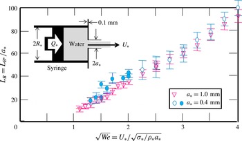
Breakup length of orifice water jets in microgravity. For each run of a four-second experiment with a prescribed dimensionless jet-issue speed
 $\sqrt{We}$
, a frequency distribution of breakup lengths was generated using high-speed charged-couple device (CCD) camera images to calculate the dimensionless average breakup length
 $L_{B}$
. Each error bar denotes the two breakup length values at half the maximum frequency. The solid circles indicate the case where the orifice exit was wetted.

Figure 1 shows the results of our parabolic flight orifice jet experiments, and will be analysed in detail in § 5. The dimensionless average breakup length
 $L_{B}=L_{B\ast }/a_{\ast }$
of a water jet (density
 ${\it\rho}_{\ast }=1~\text{g}~\text{cm}^{-3}$
and surface tension coefficient
 ${\it\sigma}_{\ast }=72~\text{dyn}~\text{cm}^{-1}$
) emanating at a prescribed speed
 $U_{\ast }$
from an orifice with radius
 $a_{\ast }$
equal to either 1 mm or 0.4 mm into still air is plotted against the dimensionless jet-issue speed
 $\sqrt{We}=U_{\ast }/V_{\ast }$
, where
 $V_{\ast }=\sqrt{{\it\sigma}_{\ast }/{\it\rho}_{\ast }a_{\ast }}$
is the jet tip contraction speed (Batchelor Reference Batchelor1958; Schulkes Reference Schulkes1996; Umemura Reference Umemura2011) and
 $We$
is the Weber number. It is known through laboratory experiments that the PR unstable wave responsible for the determination of the breakup length is produced in association with the flow instability at the injector inlet for
 $\sqrt{We}>5$
. Therefore, microgravity experiments were conducted for the jet-issue speed range
 $1<\sqrt{We}<4.5$
. The jet disintegration observed for the case
 $\sqrt{We}>\sqrt{2}$
was associated with the PR unstable wave growth. The experimental system is the same as that used for our laboratory experimental study (see details on the experimental set-up and high-speed camera image processing in Osaka et al. (Reference Osaka, Suzuki, Suzuki and Umemura2011) and Umemura & Osaka (Reference Umemura and Osaka2014)). The orifice was drilled at the centre of a stainless steel plate (thickness 0.1 mm) attached to a syringe with an inner diameter
 $2R_{\ast }=35.9~\text{mm}$
. The water pushed out by the piston separates from the leading edge of the orifice and contracts to a uniform cylindrical radius within a short distance. The contraction ratio was larger than 0.9. The jet-issue speed
 $U_{\ast }$
was estimated from the controlled piston speed
 $Q_{\ast }$
as
 $U_{\ast }=(R_{\ast }/a_{\ast })^{2}Q_{\ast }$
. In particular, the injection system was designed not to produce oscillations of jet-issue speed near the most unstable PR wave frequency. We conducted similar parabolic flight experiments in different seasons, and changed the driving motor and the syringe size
 $R_{\ast }$
. These variations in experimental conditions should produce jets with different noise, if at all. However, the resulting average breakup length had the same dependence on the speed at which jets were issued. This suggests that the initial amplitude of the PR unstable wave responsible for jet disintegration is determined by the dynamics of the issued liquid jet.
In the following sections, we develop a one-dimensional nonlinear global analysis to explain figure 1, by exploring the self-destabilising loop of the observed PR unstable wave. We also determine the initial PR unstable wave amplitude as an eigenvalue of the jet dynamics, which can be quantitatively compared to that derived from figure 1. Therefore, the global analysis developed in the present paper is different, in purpose, from the linear global analysis (Huerre & Monkewitz Reference Huerre and Monkewitz1990; Le Dizes Reference Le Dizes1997; Chomaz Reference Chomaz2005; Sauter & Buggisch Reference Sauter and Buggisch2005), in which the stability of a basic jet flow is analysed as an eigenvalue problem for the complex frequency by imposing some homogeneous boundary conditions at the upstream and downstream edges of the jet region under consideration.
2 One-dimensional low-speed water jet model
2.1 Governing equations
In our microgravity experimental runs of a water jet issued with speed
 $U_{\ast }$
from an orifice of radius
 $a_{\ast }$
, no jetting is observed at
 $\sqrt{We}<1$
(see figure 1). For
 $1<\sqrt{We}<\sqrt{2}$
, end-pinching determines the average breakup length
 $L_{B}$
. In the present paper, we consider the range
 $\sqrt{2}<\sqrt{We}<4.5$
, in which end-pinching alone cannot fix
 $L_{B}$
(Umemura Reference Umemura2011). The microgravity experiments show that PR unstable wave elements, which have a small initial amplitude, successively increase their amplitudes as they travel downstream, and disintegrate the jet at finite distances from the orifice, as shown in figure 1.
Since the jet-issue speed is not high, the effect of the surrounding still air on the jet is negligible. Viscous effects are also negligible for the water jet. Thus, to analyse the evolution of the PR unstable wave along the jet in our microgravity experiments, we adopt the inviscid one-dimensional (1-D) jet model that was first introduced by Lee (Reference Lee1974) to examine the satellite droplet formation process. Its modified versions have recently been used for other purposes as well (Eggers & Dupont Reference Eggers and Dupont1994; Ambravaneswaran et al.
Reference Ambravaneswaran, Subramani, Phillops and Basaran2004; Rubio-Rubio, Sevilla & Gordillo Reference Rubio-Rubio, Sevilla and Gordillo2013). In the 1-D model, it is assumed that the cross-sectional hydrodynamic properties are uniform at each location along the jet (Weber Reference Weber1931). Therefore, measuring the distance
 $x_{\ast }$
from the orifice exit along the jet centreline, the instantaneous jet flow is described by the surface radius
 $r_{\ast }(t_{\ast },x_{\ast })$
, axial velocity
 $u_{\ast }(t_{\ast },x_{\ast })$
and pressure
 $p_{\ast }(t_{\ast },x_{\ast })$
. Defining the dimensionless variables
 $t=t_{\ast }U_{\ast }/a_{\ast }$
,
 $x=x_{\ast }/a_{\ast }$
,
 $r=r_{\ast }/a_{\ast }$
,
 $u=u_{\ast }/U_{\ast }$
and
 $p=p_{\ast }a_{\ast }/{\it\sigma}_{\ast }$
, the continuity equation and unsteady Bernoulli’s equation along the jet centreline are expressed as
 $$\begin{eqnarray}{\displaystyle \frac{\partial r}{\partial t}}+u{\displaystyle \frac{\partial r}{\partial x}}=-{\displaystyle \frac{r}{2}}{\displaystyle \frac{\partial u}{\partial x}}\end{eqnarray}$$
 $$\begin{eqnarray}{\displaystyle \frac{\partial u}{\partial t}}+u{\displaystyle \frac{\partial u}{\partial x}}=-{\displaystyle \frac{\partial p}{\partial x}},\quad p={\displaystyle \frac{1}{We}}\left[{\displaystyle \frac{1}{r\sqrt{1+\left({\displaystyle \frac{\partial r}{\partial x}}\right)^{2}}}}-{\displaystyle \frac{{\displaystyle \frac{\partial ^{2}r}{\partial x^{2}}}}{\left\{1+\left({\displaystyle \frac{\partial r}{\partial x}}\right)^{2}\right\}\sqrt{1+\left({\displaystyle \frac{\partial r}{\partial x}}\right)^{2}}}}\right].\end{eqnarray}$$
In a two-dimensional (2-D) jet model that accounts for the internal jet-flow structure as an axisymmetric potential flow, (2.1) and (2.2) are respectively replaced by the kinematic condition and unsteady Bernoulli’s equation applied at the jet surface. These serve as the boundary conditions for the potential jet-flow field. Compared to this 2-D model, the 1-D model has advantages in eliminating difficulties associated with the infinite degrees of freedom of the internal jet-flow structure and in facilitating the elucidation of physical and mathematical aspects in the present problem. It is documented that the 1-D model can accurately describe relatively long wave phenomena (PR unstable wave evolution and end-pinching) (Umemura Reference Umemura2011). However, it is obvious that the approximation of short waves is degraded. Resulting differences between the two models will be discussed and 2-D model corrections will be made, leading to the final result presented in § 4.
2.2 Regular perturbation expansion equation system
In the experiments, all water jets appear to be almost smooth uniform liquid cylinders in a near-orifice region. The steady solutions of (2.1) and (2.2) subject to the orifice exit condition
 $r=u=1$
at
 $x=0$
can be expressed as
 $r^{2}u=1$
and
 $$\begin{eqnarray}\displaystyle {\displaystyle \frac{1}{\sqrt{1+\left(\text{d}r/\text{d}x\right)^{2}}}} & = & \displaystyle {\displaystyle \frac{We}{4}}\!\left(\!r+{\displaystyle \frac{1}{r^{3}}}-2{\displaystyle \frac{1}{r}}\right)+{\displaystyle \frac{1}{2}}\!\left[\!{\displaystyle \frac{1}{\sqrt{1+\left(\text{d}r/\text{d}x|_{x=0}\right)^{2}}}}-{\displaystyle \frac{\text{d}^{2}r/\text{d}x^{2}|_{x=0}}{\{1+(\text{d}r/\text{d}x|_{x=0})^{2}\}}}\right]\nonumber\\ \displaystyle & & \displaystyle \times \,\left(r-{\displaystyle \frac{1}{r}}\right)+{\displaystyle \frac{1}{r\sqrt{1+1+(\text{d}r/\text{d}x|_{x=0})^{2}}}}\leqslant 1.\end{eqnarray}$$
These equations indicate that the steady jet flow, which satisfies
 $\text{d}r/\text{d}r=\text{d}^{2}r/\text{d}x^{2}=0$
at
 $x=0$
and the last inequality of (2.3), is the uniform jet
 $(r=1,u=1)$
only. Therefore, we set
 $$\begin{eqnarray}r=1+{\it\delta},\quad u=1+v.\end{eqnarray}$$
The conventional perturbation expansion approach starts by introducing a small dimensionless parameter
 ${\it\varepsilon}_{ref}$
, which characterises the magnitude of the jet surface deformation in the near-orifice region. Technically,
 ${\it\varepsilon}_{ref}$
could be defined as the amplitude of
 ${\it\delta}$
at a certain distance from the orifice exit (later, we will redefine
 ${\it\varepsilon}_{ref}$
in a more convenient form). This value should be small, but in general it cannot be known a priori.
Given a small parameter
 ${\it\varepsilon}_{ref}\ll 1$
,
 ${\it\delta}$
and
 $v$
are expanded into a power series in
 ${\it\varepsilon}_{ref}$
as
 $$\begin{eqnarray}{\it\delta}={\it\varepsilon}_{ref}{\it\delta}_{1}+{\it\varepsilon}_{ref}^{2}{\it\delta}_{2}+{\it\varepsilon}_{ref}^{3}{\it\delta}_{3}+\cdots \,,\quad v={\it\varepsilon}_{ref}v_{1}+{\it\varepsilon}_{ref}^{2}v_{2}+{\it\varepsilon}_{ref}^{3}v_{3}+\cdots \,.\end{eqnarray}$$
The following perturbation equations are derived for each order (
 $n\text{th}$
) of the perturbation variable up to the third power of
 ${\it\varepsilon}_{ref}$
.
 $$\begin{eqnarray}\displaystyle & \text{Continuity equation:}\quad {\displaystyle \frac{\partial {\it\delta}_{n}}{\partial t}}+{\displaystyle \frac{\partial {\it\delta}_{n}}{\partial x}}+{\displaystyle \frac{1}{2}}{\displaystyle \frac{\partial v_{n}}{\partial x}}=F_{n} & \displaystyle\end{eqnarray}$$
 $$\begin{eqnarray}\displaystyle & \text{Momentum equation:}\quad {\displaystyle \frac{\partial v_{n}}{\partial t}}+{\displaystyle \frac{\partial v_{n}}{\partial x}}-{\displaystyle \frac{1}{We}}{\displaystyle \frac{\partial {\it\delta}_{n}}{\partial x}}-{\displaystyle \frac{1}{We}}{\displaystyle \frac{\partial ^{3}{\it\delta}_{n}}{\partial x^{3}}}=G_{n} & \displaystyle\end{eqnarray}$$
We note that
 $F_{1}=G_{1}=0.$
The expressions for
 $F_{n}$
and
 $G_{n}$
(
 $n=2$
and 3) are given in appendix A.
3 Linear spatial evolution analysis
The purpose of the present perturbation expansion approach is to reveal why jet disintegration occurs at locations near an average breakup length determined by the jet-issue speed. To do this, we consider an idealised case, whereby the jet disintegrates periodically in time at an angular frequency
 ${\it\omega}>0$
at the average breakup length location. Also, we analyse this case in the framework of the spatial evolution analysis. The actual jet deformation is not completely periodic in time. Deviation from the idealised case will be discussed in § 5, after (2.6) and (2.7) have been solved for the idealised case. In this section, we consider the near-orifice region and clarify the physical meaning of the small parameter
 ${\it\varepsilon}_{ref}$
in our spatial evolution analysis.
3.1 Dispersion relation
To determine the frequency
 ${\it\omega}$
at which the PR unstable wave is excited at the orifice exit, we first consider the solution of the first-order (
 $n=1$
) equations (2.6) and (2.7) that describe the small jet deformation in the near-orifice region
 $0<x<X$
. This 1-D jet model solution was first derived by Pimbley (Reference Pimbley1976) and Pimbley & Lee (Reference Pimbley and Lee1977) to analyse droplet formation from a liquid jet in their boundary value problems by solving the perturbation equations (2.6) and (2.7) to second order.
Using complex expressions, we set
 $$\begin{eqnarray}{\it\delta}_{1}=A\text{e}^{\text{i}kx-\text{i}{\it\omega}t}+\bar{A}\text{e}^{-\text{i}\bar{k}x+\text{i}{\it\omega}t},\quad v_{1}=B\text{e}^{\text{i}kx-\text{i}{\it\omega}t}+\bar{B}\text{e}^{-\text{i}\bar{k}x+\text{i}{\it\omega}t}.\end{eqnarray}$$
Equations (2.6) and (2.7) lead to
 $$\begin{eqnarray}(-{\it\omega}+k)A+{\displaystyle \frac{1}{2}}kB=0\quad \text{and}\quad (-{\it\omega}+k)B-{\displaystyle \frac{1}{We}}k(1-k^{2})A=0,\end{eqnarray}$$
which yield the dispersion relation
 $$\begin{eqnarray}D(k,{\it\omega})=(-{\it\omega}+k)^{2}+{\displaystyle \frac{1}{2We}}k^{2}\left(1-k^{2}\right)=0.\end{eqnarray}$$
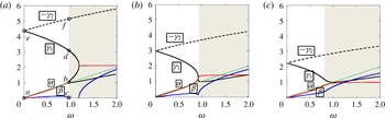
Waves excitable for an inviscid liquid jet: (a)
 $\sqrt{We}=3$
, (b)
 $\sqrt{We}=2$
, (c)
 $\sqrt{We}=\sqrt{2}$
. The four roots
 $k$
are expressed as functions of the frequency
 ${\it\omega}$
. Black solid and dashed lines represent neutral waves. The real and imaginary parts of the complex wavenumber are represented by red and blue lines, respectively. Each complex conjugate wave has a blue line symmetry with respect to the
 ${\it\omega}$
axis. On the thin green solid line, the phase velocity coincides with the jet velocity. The
 $\sqrt{We}=3$
case represents topology of the roots at
 $\sqrt{We}>2$
. No PR unstable wave emerges in the grey region. Symbols
 ${\it\gamma}_{1},{\it\gamma}_{2},{\it\alpha}$
and
 ${\it\beta}$
are assigned to distinguish the four roots in the frequency range where the PR unstable wave may emerge.

For a prescribed jet-issue speed
 $\sqrt{We}$
and frequency
 ${\it\omega}$
, (3.3) has four roots
 $k$
, as shown in figure 2. In our problem, each root (
 $k$
) must represent a wave mode (
 $\text{e}^{\text{i}kx-\text{i}{\it\omega}t}$
) which is excited by a periodic forcing at the orifice exit or downstream of the near-orifice region. Causality considerations (Briggs Reference Briggs1964; Huerre & Monkewitz Reference Huerre and Monkewitz1990) are necessary to identify those wave modes which are excitable in our microgravity experiments for
 $\sqrt{2}<\sqrt{We}<4.5$
, in which all water jets are disintegrated by the growth of PR unstable waves. From figure 2, it is found that, together with its complex conjugate (subdominant mode) wave, the PR unstable wave (
 $k={\it\alpha}-\text{i}{\it\beta}$
) is excitable at the orifice exit in a low-frequency range. The spatial growth rate
 ${\it\beta}$
is maximised when the dimensionless phase velocity
 ${\it\omega}/{\it\alpha}$
becomes almost equal to unity. Hence, assuming that
 ${\it\omega}/{\it\alpha}=1$
for
 $k={\it\alpha}-\text{i}{\it\beta}$
in (3.3), the dependencies of
 ${\it\alpha}$
and
 ${\it\beta}$
of the most unstable waves on
 $\sqrt{We}$
are analytically expressed as
 $$\begin{eqnarray}{\it\alpha}=\sqrt{{\displaystyle \frac{We+1-\sqrt{We^{2}-2We}}{4}}},\quad {\it\beta}=\sqrt{{\displaystyle \frac{We-1-\sqrt{We^{2}-2We}}{4}}}.\end{eqnarray}$$
This indicates that the most unstable PR wave may emerge at jet-issue speeds
 $\sqrt{We}>\sqrt{2}$
. It is also noted that the most unstable PR wave predicted from the 1-D model is highly accurate and consistent with the plug flow jet solution obtained by Keller et al. (Reference Keller, Ubinow and Tu1973), Leib & Goldstein (Reference Leib and Goldstein1986) and Guerrero, Gonzalez & Garcia (Reference Guerrero, Gonzalez and Garcia2012), who treated the 2-D model. The other waves, which are excitable in the same frequency range, are the two neutral waves with an upstream propagation speed (labelled de:
 ${\it\gamma}_{1}$
and ef:
 $-{\it\gamma}_{2}$
); one (de) moves downstream whereas the other (ef) moves upstream. Since these waves can transfer energy in the upstream direction without loss, they must be excited at
 $x>X$
. In appendix B, it is explained how these neutral waves are established from the upstream propagating dispersive wave produced by an impulsive/periodic point forcing.
When analytical continuation of the dispersion relation (3.3) is considered, the absolute instability identified with a saddle point
 $\text{d}{\it\omega}/\text{d}k=0$
with
 ${\it\omega}_{i}>0$
(Monkewitz et al.
Reference Monkewitz, Davis, Bojorquez and Yu1988; Lin & Lian Reference Lin and Lian1989; Monkewitz Reference Monkewitz1990; Vihinen, Honohan & Lin Reference Vihinen, Honohan and Lin1997; O’Donnell, Chen & Lin Reference O’Donnell, Chen and Lin2001) emerges at
 $\sqrt{We}<\sqrt{2}$
. This saddle point represents a transient wave state associated with an interaction between two waves produced by a certain frequency of forcing at
 $x=0$
and
 $x>X$
. For the temporally periodic waves under consideration, there remains a PR unstable wave solution in a narrowed frequency range lower than the saddle point frequency (see figure 2
c). Our experimental observations indicated that the jet disintegration is caused by the PR unstable wave growth, even at
 $\sqrt{2}<\sqrt{We}<2$
, although the jet tip contraction effect becomes evident as
 $\sqrt{We}$
approaches
 $\sqrt{2}$
.
3.2 The two solution types that allow PR unstable wave excitation
For a small value of
 ${\it\varepsilon}_{ref}$
, the near-orifice jet deformation is expressed as a linear combination of the four wave modes explained in § 3.1. We seek a general solution that satisfies the boundary conditions at the orifice exit. Since we are interested in convective instability, the general solution must include a PR unstable wave of wavenumber
 $k={\it\alpha}-\text{i}{\it\beta}$
(
 ${\it\alpha},{\it\beta}>0$
). This confines the allowable frequency
 ${\it\omega}$
in a restricted range, at which a PR unstable wave is excitable for each
 $\sqrt{We}$
, along with two neutral waves of wavenumbers
 $k={\it\gamma}_{1}>0$
and
 $k={\it\gamma}_{2}<0$
.
If the jet-issue speed changes periodically according to
 $1+{\rm\Delta}U\sin ({\it\omega}t)$
, a PR unstable wave of frequency
 ${\it\omega}$
is generated at the orifice exit
 $x=0$
. To describe such a process with the 1-D model, we follow Pimbley (Reference Pimbley1976) and use all four wave modes relevant to the considered frequency to satisfy the boundary conditions at
 $x=0$
and
 $x=X$
, although the downstream boundary location
 $X$
and the
 ${\it\varepsilon}_{ref}{\it\delta}_{1}$
and
 ${\it\varepsilon}_{ref}v_{1}$
values there must be left unspecified.
Thus, introducing four arbitrary complex constants
 $C_{1}{-}C_{4}$
, the first-order perturbation surface deformation
 ${\it\varepsilon}_{ref}{\it\delta}_{1}$
and axial velocity
 ${\it\varepsilon}_{ref}v_{1}$
for given
 $\sqrt{We}$
and
 ${\it\omega}$
are generally expressed in the following forms:
 $$\begin{eqnarray}{\it\varepsilon}_{ref}{\it\delta}_{1}=C_{1}\text{e}^{\text{i}{\it\gamma}_{1}x-\text{i}{\it\omega}t}+C_{2}\text{e}^{\text{i}{\it\gamma}_{2}x-\text{i}{\it\omega}t}+C_{3}\text{e}^{\text{i}\left({\it\alpha}-\text{i}{\it\beta}\right)x-\text{i}{\it\omega}t}+C_{4}\text{e}^{\text{i}\left({\it\alpha}+\text{i}{\it\beta}\right)x-\text{i}{\it\omega}t}+\text{c.c.},\end{eqnarray}$$
 $$\begin{eqnarray}\displaystyle {\it\varepsilon}_{ref}v_{1} & = & \displaystyle 2\left({\displaystyle \frac{{\it\omega}}{{\it\gamma}_{1}}}-1\right)C_{1}\text{e}^{\text{i}{\it\gamma}_{1}x-\text{i}{\it\omega}t}+2\left({\displaystyle \frac{{\it\omega}}{{\it\gamma}_{2}}}-1\right)C_{2}\text{e}^{\text{i}{\it\gamma}_{2}x-\text{i}{\it\omega}t}\nonumber\\ \displaystyle & & \displaystyle +\,2\left({\displaystyle \frac{{\it\omega}}{{\it\alpha}-\text{i}{\it\beta}}}-1\right)C_{3}\text{e}^{\text{i}\left({\it\alpha}-\text{i}{\it\beta}\right)x-\text{i}{\it\omega}t}\nonumber\\ \displaystyle & & \displaystyle +\,2\left({\displaystyle \frac{{\it\omega}}{{\it\alpha}+\text{i}{\it\beta}}}-1\right)C_{4}\text{e}^{\text{i}\left({\it\alpha}+\text{i}{\it\beta}\right)x-\text{i}{\it\omega}t}+\text{c.c.}\end{eqnarray}$$
Applying the boundary conditions
 ${\it\varepsilon}_{ref}{\it\delta}_{1}(x=0)=0$
and
 ${\it\varepsilon}_{ref}v_{1}(x=0)={\rm\Delta}U\sin ({\it\omega}t)$
(note that the imposed boundary conditions are different from those in Pimbley (Reference Pimbley1976)), we obtain in general the following expressions for a PR unstable wave evolution:
 $$\begin{eqnarray}\displaystyle & \displaystyle {\it\varepsilon}_{ref}{\it\delta}_{1}={\it\varepsilon}_{ref}{\it\delta}_{{\rm\Delta}U}+{\it\varepsilon}_{ref}{\it\delta}_{{\it\varepsilon}_{1}}+{\it\varepsilon}_{ref}{\it\delta}_{{\it\varepsilon}_{2}}, & \displaystyle\end{eqnarray}$$
 $$\begin{eqnarray}\displaystyle & \displaystyle {\it\varepsilon}_{ref}{\it\delta}_{{\rm\Delta}U}={\displaystyle \frac{{\it\alpha}^{2}+{\it\beta}^{2}}{2{\it\beta}}}{\displaystyle \frac{{\rm\Delta}U}{{\it\omega}}}\sinh {\it\beta}x\cos \left({\it\alpha}x-{\it\omega}t\right), & \displaystyle\end{eqnarray}$$
 $$\begin{eqnarray}\displaystyle {\it\varepsilon}_{ref}{\it\delta}_{{\it\varepsilon}_{n}} & = & \displaystyle 2{\it\varepsilon}_{n}\left\{\left({\displaystyle \frac{{\it\alpha}^{2}+{\it\beta}^{2}}{{\it\gamma}_{n}{\it\beta}}}-{\displaystyle \frac{{\it\alpha}}{{\it\beta}}}\right)\sinh {\it\beta}x\sin ({\it\alpha}x-{\it\omega}t+{\it\theta}_{n})\right.\nonumber\\ \displaystyle & & \displaystyle \left.+\,\cosh {\it\beta}x\cos ({\it\alpha}x-{\it\omega}t+{\it\theta}_{n})-\cos \left({\it\gamma}_{n}x-{\it\omega}t+{\it\theta}_{n}\right)\right\}.\end{eqnarray}$$
Herein,
 $n=1$
and 2. Correspondingly,
 ${\it\varepsilon}_{n}$
and
 ${\it\theta}_{n}$
denote a small arbitrary amplitude and phase difference, respectively. The corresponding expressions for
 ${\it\varepsilon}_{ref}v_{1}$
are also derived, but these are omitted for brevity.
Equation (3.7) expresses two kinds of solution explained below.
3.2.1 Conventional theory
Equation (3.8) represents the PR unstable wave which is produced as a result of the oscillation of jet-issue speed. The unstable wave grows along the jet, and disintegrates the jet. For a small value of
 ${\rm\Delta}U$
, which justifies the perturbation expansion approach in § 2, the near-orifice region, to which (3.8) is applicable, occupies a large fraction of the breakup length
 $L_{B}$
. Therefore, if
 ${\it\varepsilon}_{1}={\it\varepsilon}_{2}=0$
, solving
 ${\it\varepsilon}_{ref}{\it\delta}_{{\rm\Delta}U}(x=L_{B})=1$
in (3.8), we obtain the following approximate expression for the breakup length:
 $$\begin{eqnarray}\displaystyle L_{B}={\displaystyle \frac{1}{{\it\beta}}}\ln {\displaystyle \frac{1}{{\it\varepsilon}_{0}}}\quad \text{with }{\it\varepsilon}_{0}\equiv {\displaystyle \frac{{\it\alpha}^{2}+{\it\beta}^{2}}{4{\it\beta}{\it\omega}}}{\rm\Delta}U. & & \displaystyle\end{eqnarray}$$
When
 ${\rm\Delta}U$
is not a prescribed quantity,
 ${\it\varepsilon}_{0}$
may be considered to represent a noise contribution. Equations (3.7), (3.9) and (3.10) indicate that unless
 ${\it\varepsilon}_{1}={\it\varepsilon}_{2}=0$
or
 ${\it\varepsilon}_{n}<{\it\varepsilon}_{0}$
, the conventionally used expression (3.10) is not applicable. To ensure the applicability of the condition
 ${\it\varepsilon}_{n}<{\it\varepsilon}_{0}$
, we need to introduce a theoretical framework that enables the estimation of the magnitude of the unknown amplitude
 ${\it\varepsilon}_{n}$
. This is an unnoticed difficulty that is not described well in the conventional theory.
3.2.2 Self-destabilisation theory
When
 ${\rm\Delta}U$
is relatively large, the jet disintegrates within a short distance. As
 ${\rm\Delta}U$
decreases, the region where (3.8) is applicable is lengthened, and the breakup length
 $L_{B}$
increases correspondingly. However, even if
 ${\rm\Delta}U=0$
, there is still (3.9), which includes the same type of PR unstable wave as well as a neutral wave represented by
 $2{\it\varepsilon}_{n}\cos ({\it\gamma}_{n}x-{\it\omega}t+{\it\theta}_{n})$
. As a result, if there is a mechanism which renders
 ${\it\varepsilon}_{n}$
non-zero, the jet disintegrates due to the growth of the PR unstable wave. To predict this breakup length, we have to understand the physical implication of (3.9) and identify how the magnitude of
 ${\it\varepsilon}_{n}$
is determined. Therefore, in the subsequent sections, we focus our attention on the case where
 ${\rm\Delta}U=0$
.
We transform (3.7) (with
 ${\rm\Delta}U=0$
) to a suitable form for subsequent analyses. The PR unstable wave excitation accompanies the subdominant mode wave (complex conjugate root), which attenuates rapidly away from the orifice. This contribution can be eliminated when we use (3.7) evaluated at location
 $x$
, where
 $\text{e}^{-2{\it\beta}x}\ll 1$
, and both
 $\cosh ({\it\beta}x)$
and
 $\sinh ({\it\beta}x)$
are approximated as
 $0.5\text{e}^{{\it\beta}x}$
. Then, using the addition theorem of trigonometric functions, (3.7) can be rewritten as indicated below. The arbitrary constants
 ${\it\varepsilon}_{n}$
are rewritten so as to express the initial amplitude (
 ${\it\varepsilon}_{n}^{\prime }$
or
 ${\it\varepsilon}$
) of a PR unstable wave.
 $$\begin{eqnarray}\displaystyle {\it\varepsilon}_{ref}{\it\delta}_{1} & = & \displaystyle {\it\varepsilon}_{1}^{\prime }\left[\text{e}^{{\it\beta}x}\cos \left({\it\alpha}x-{\it\omega}t-{\it\Theta}_{1}^{\prime }\right)-2K_{1}^{\prime }\cos \left({\it\gamma}_{1}x-{\it\omega}t+{\it\theta}_{1}\right)\right]\end{eqnarray}$$
 $$\begin{eqnarray}\displaystyle & & \displaystyle +\,{\it\varepsilon}_{2}^{\prime }\left[\text{e}^{{\it\beta}x}\cos \left({\it\alpha}x-{\it\omega}t-{\it\Theta}_{2}^{\prime }\right)-2K_{2}^{\prime }\cos \left({\it\gamma}_{1}x-{\it\omega}t+{\it\theta}_{2}\right)\right]\end{eqnarray}$$
 $$\begin{eqnarray}\displaystyle & = & \displaystyle {\it\varepsilon}\left[\text{e}^{{\it\beta}x}\cos \left({\it\alpha}x-{\it\omega}t-{\it\Theta}\right)-2K_{1}\cos \left({\it\gamma}_{1}x-{\it\omega}t+{\it\theta}_{1}\right)-2K_{2}\cos \left({\it\gamma}_{2}x-{\it\omega}t+{\it\theta}_{2}\right)\right]\!.\nonumber\\ \displaystyle & & \displaystyle\end{eqnarray}$$
 $$\begin{eqnarray}K_{n}^{\prime }=1\left/\sqrt{\left({\displaystyle \frac{{\it\alpha}^{2}+{\it\beta}^{2}}{{\it\gamma}_{n}{\it\beta}}}\right)^{2}+1}\right..\end{eqnarray}$$
The arbitrary constants are transformed as
 $$\begin{eqnarray}{\it\varepsilon}_{n}^{\prime }={\displaystyle \frac{{\it\varepsilon}_{n}}{K_{n}^{\prime }}},\quad {\it\Theta}_{n}^{\prime }=\tan ^{-1}\left({\displaystyle \frac{{\it\alpha}^{2}+{\it\beta}^{2}}{{\it\gamma}_{n}{\it\beta}}}-{\displaystyle \frac{{\it\alpha}}{{\it\beta}}}\right)-{\it\theta}_{n}.\end{eqnarray}$$
In (3.13),
 $$\begin{eqnarray}{\it\varepsilon}=\sqrt{{\it\varepsilon}_{1}^{\prime 2}+{\it\varepsilon}_{2}^{\prime 2}+2{\it\varepsilon}_{1}^{\prime }{\it\varepsilon}_{2}^{\prime }\cos \left({\it\Theta}_{1}^{\prime }-{\it\Theta}_{2}^{\prime }\right)},\quad {\it\Theta}=\tan ^{-1}{\displaystyle \frac{{\it\varepsilon}_{1}^{\prime }\sin \left({\it\Theta}_{1}^{\prime }\right)+{\it\varepsilon}_{2}^{\prime }\sin \left({\it\Theta}_{2}^{\prime }\right)}{{\it\varepsilon}_{1}^{\prime }\cos \left({\it\Theta}_{1}^{\prime }\right)+{\it\varepsilon}_{2}^{\prime }\cos \left({\it\Theta}_{2}^{\prime }\right)}}.\end{eqnarray}$$
 $K_{n}$
is defined so as to satisfy the relations
 $$\begin{eqnarray}{\it\varepsilon}_{n}=K_{n}^{\prime }{\it\varepsilon}_{n}^{\prime }=K_{n}{\it\varepsilon}.\end{eqnarray}$$
The expressions (3.11) and (3.12) will be used in § 4.3. In all prior analyses, we use (3.13) only.
Each neutral wave included in (3.13) can transfer energy from downstream to upstream, and thereby to the newly issued water. This means that the neutral waves must be produced downstream of the region where (3.13) is applicable. At the same time, the spatial evolution solution (3.13) is interpreted to express such a process that the PR unstable wave is produced at the orifice exit by complete reflection of the neutral waves. Therefore, if the neutral waves are produced by the nonlinear growth of the PR unstable wave, (3.13) expresses the reproduction of the PR unstable wave by itself.
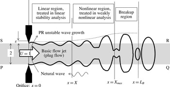
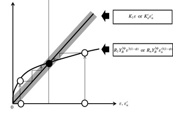
In § 4, the possibility of this self-destabilising loop formation is examined, by analysing the jet surface deformation downstream of the near-orifice region, in the framework of the weakly nonlinear analysis presented in § 2.2. Figure 3 illustrates the scope of this weakly nonlinear analysis. In general, the jet-disintegration location depends on
 $\sqrt{We}$
,
 ${\it\omega}$
and
 ${\it\varepsilon}$
. The range,
 $0<x<X$
, where (3.13) holds to a good degree of approximation is lengthened for a smaller value of
 ${\it\varepsilon}$
. This region is called the ‘linear region’ in the present paper. Each wave mode determined from the dispersion relation can be mathematically defined over an infinitely long, hypothetical basic flow region (grey region in figure 3), but physically it is not. The nonlinear growth of the PR unstable wave downstream of the linear region is described by the higher-order perturbation equations, which will produce upstream propagating dispersive waves in general. It will be shown that the magnitude of
 ${\it\varepsilon}$
can be self-consistently determined using the weakly nonlinear analysis result.
Spatial evolution of a low-speed liquid jet deformation. Each root of the dispersion relation derived from the linear stability analysis represents the perturbation wave in the linear region, which may be excited by a periodic forcing outside of the linear region. The dashed line denotes the growth in amplitude of the linear PR unstable wave and a saturated surface deformation amplitude in the breakup region. Mathematically, the linear stability analysis solutions can be defined over an infinitely long, hypothetical basic flow jet (grey region PQRS).

3.3 Predominant unstable wave
The expression (3.10a
) suggests that the breakup length is primarily determined by the magnitude of the spatial growth rate
 ${\it\beta}$
rather than the initial unstable wave amplitude
 ${\it\varepsilon}$
involved in the logarithmic function. Thus, for a given value of
 $\sqrt{We}$
, the PR unstable wave of the frequency that maximises the spatial growth rate (and thereby minimises the linear region length) disintegrates the jet at the shortest distance from the orifice. This implies that the PR unstable waves of other frequencies, which would exhibit significant nonlinear growth at locations beyond the shortest breakup length, cannot establish an effective self-destabilising loop. Therefore, only the PR unstable wave and neutral waves of the predominant frequency are considered in the following sections, and all numerical estimations are based on (3.4a,b
). The real wavenumber
 ${\it\gamma}_{n}$
for
 ${\it\omega}={\it\alpha}$
is calculated numerically from the dispersion relation.
4 Self-excitation of the PR unstable wave in the spatial analysis
4.1 Perturbation equations for the nonlinear unstable wave growth
Using (2.6) and (2.7), we examine the nonlinear evolution of the PR unstable wave included in (3.13) by substituting
 ${\it\varepsilon}_{ref}={\it\varepsilon}$
,
 $$\begin{eqnarray}{\it\delta}_{1}={\it\delta}_{1,PR}=A\text{e}^{{\it\beta}x+\text{i}({\it\alpha}x-{\it\omega}t-{\it\Theta})}+\text{c.c.}\quad \text{with }A={\textstyle \frac{1}{2}}\end{eqnarray}$$
and
 $$\begin{eqnarray}v_{1}=v_{1,PR}=B\text{e}^{{\it\beta}x+\text{i}\left({\it\alpha}x-{\it\omega}t-{\it\Theta}\right)}+\text{c.c.}\quad \text{with }B=2\left({\displaystyle \frac{{\it\omega}}{{\it\alpha}-\text{i}{\it\beta}}}-1\right)A.\end{eqnarray}$$
Since the PR unstable wave increases its amplitude exponentially according to
 ${\it\varepsilon}\text{e}^{{\it\beta}x}$
, the magnitudes of the solutions
 ${\it\varepsilon}^{m}{\it\delta}_{m}$
and
 ${\it\varepsilon}^{m}u_{m}\;(m=1,2,3)$
change significantly along the jet. Nevertheless, if
 ${\it\varepsilon}$
satisfies the PR unstable wave amplitude
 $Y\equiv {\it\varepsilon}\text{e}^{{\it\beta}x}<1$
at any location
 $x$
under consideration, the same form of the regular perturbation expansion equation system can be constructed for a local disturbed flow field about each location
 $x$
, by regarding
 $Y$
(which is larger than
 ${\it\varepsilon}$
but smaller than unity) as the small expansion parameter (Umemura Reference Umemura2014). Therefore, (2.6) and (2.7) are valid at all locations except for a region near the jet-disintegration location.
It is well known that the third-order equations lead to those waves which have the same time dependence as the first-order solution. Derivation of the third-order equations is detailed in appendix A. Substituting (4.1) and (4.2) into the inhomogeneous terms
 $F_{2}$
and
 $G_{2}$
of the second-order equations (2.6) and (2.7), we can obtain the particular solutions proportional to
 $\text{e}^{2{\it\beta}x}$
, which dominate the second-order solutions
 $({\it\delta}_{2},v_{2})$
, with the exception of the region near the orifice. Thus, the inhomogeneous terms of the third-order equations are expressed in terms of the first-order solutions and the second-order particular solutions. Among them, we select those terms which have the same time dependence as the first-order solution. We can thus obtain
 $$\begin{eqnarray}\displaystyle & {\displaystyle \frac{\partial {\it\delta}_{3}}{\partial t}}+{\displaystyle \frac{\partial {\it\delta}_{3}}{\partial x}}+{\displaystyle \frac{1}{2}}{\displaystyle \frac{\partial v_{3}}{\partial x}}=\text{i}S_{{\it\delta}}\text{e}^{3{\it\beta}x}\text{e}^{\text{i}\left({\it\alpha}x-{\it\omega}t-{\it\Theta}\right)}+\text{c.c.} & \displaystyle\end{eqnarray}$$
 $$\begin{eqnarray}\displaystyle & {\displaystyle \frac{\partial v_{3}}{\partial t}}+{\displaystyle \frac{\partial v_{3}}{\partial x}}-{\displaystyle \frac{1}{We}}\left({\displaystyle \frac{\partial {\it\delta}_{3}}{\partial x}}+{\displaystyle \frac{\partial ^{3}{\it\delta}_{3}}{\partial x^{3}}}\right)=\text{i}S_{u}\text{e}^{3{\it\beta}x}\text{e}^{\text{i}({\it\alpha}x-{\it\omega}t-{\it\Theta})}+\text{c.c.} & \displaystyle\end{eqnarray}$$
The expressions for
 $S_{{\it\delta}}({\it\alpha},{\it\beta};We)$
and
 $S_{u}({\it\alpha},{\it\beta};We)$
are presented in appendix A. The nonlinear PR unstable wave growth of
 $O({\it\varepsilon}^{2})$
and
 $O({\it\varepsilon}^{3})$
may produce other harmonic waves in the linear region, but such waves are not involved in the formation of the PR unstable wave at the orifice exit to
 $O({\it\varepsilon}^{3})$
.
4.2 First-order neutral waves produced by nonlinear PR unstable wave growth
We are interested in the temporally varying solutions expressed in the form
 ${\it\delta}_{n}=\tilde{{\it\delta}}_{n}(x)\text{e}^{-\text{i}{\it\omega}t}+\text{c.c.}\;(n=1,3)$
. Eliminating
 $v_{3}$
from (4.3) and (4.4), the ordinary differential equation for
 $\tilde{{\it\delta}}_{3}$
is derived as
 $$\begin{eqnarray}\left[-\left(-\text{i}{\it\omega}+{\displaystyle \frac{\text{d}}{\text{d}x}}\right)^{2}-{\displaystyle \frac{1}{2We}}{\displaystyle \frac{\text{d}^{2}}{\text{d}x^{2}}}\left(1+{\displaystyle \frac{\text{d}^{2}}{\text{d}x^{2}}}\right)\right]{\it\varepsilon}^{3}\tilde{{\it\delta}}_{3}={\it\varepsilon}^{3}\text{i}S\text{e}^{(3{\it\beta}+\text{i}{\it\alpha})x-\text{i}{\it\Theta}}+\text{c.c.}\end{eqnarray}$$
with
 $$\begin{eqnarray}S={\textstyle \frac{1}{2}}(3{\it\beta}+\text{i}{\it\alpha})S_{u}-\{-\text{i}{\it\omega}+(3{\it\beta}+\text{i}{\it\alpha})\}S_{{\it\delta}}.\end{eqnarray}$$
The inhomogeneous term of (4.5) may excite an upstream propagating neutral wave of
 $O({\it\varepsilon})$
near the orifice exit. To capture such first-order waves (other than the PR unstable wave), we consider the following first-order equation as well:
 $$\begin{eqnarray}\left[-\left(-\text{i}{\it\omega}+{\displaystyle \frac{\text{d}}{\text{d}x}}\right)^{2}-{\displaystyle \frac{1}{2We}}{\displaystyle \frac{\text{d}^{2}}{\text{d}x^{2}}}\left(1+{\displaystyle \frac{\text{d}^{2}}{\text{d}x^{2}}}\right)\right]{\it\varepsilon}(\tilde{{\it\delta}}_{1}-\tilde{{\it\delta}}_{1,PR})=0.\end{eqnarray}$$
Setting
 $$\begin{eqnarray}\tilde{{\it\delta}}_{1+3}={\it\varepsilon}(\tilde{{\it\delta}}_{1}-\tilde{{\it\delta}}_{1,PR})+{\it\varepsilon}^{3}\tilde{{\it\delta}}_{3},\end{eqnarray}$$
equations (4.5) and (4.7) are combined to yield
 $$\begin{eqnarray}\left[-\left(-\text{i}{\it\omega}+{\displaystyle \frac{\text{d}}{\text{d}x}}\right)^{2}-{\displaystyle \frac{1}{2We}}{\displaystyle \frac{\text{d}^{2}}{\text{d}x^{2}}}\left(1+{\displaystyle \frac{\text{d}^{2}}{\text{d}x^{2}}}\right)\right]\tilde{{\it\delta}}_{1+3}={\it\varepsilon}^{3}\text{i}S\text{e}^{(3{\it\beta}+\text{i}{\it\alpha})x-\text{i}{\it\Theta}}+\text{c.c.}\end{eqnarray}$$
This equation can be solved for the complex function
 $\tilde{{\it\delta}}_{1+3}$
, as described below.
As illustrated in figure 3, we consider a location
 $x=X_{max}<L_{B}$
. Equation (4.9) holds in the region
 $0<x\leqslant X_{max}$
. Nevertheless, if we ignore the presence of the orifice at
 $x=0$
and confine ourselves to those waves produced by the forcing (inhomogeneous term)
 $$\begin{eqnarray}f=\left\{\begin{array}{@{}l@{}}{\it\varepsilon}^{3}\text{i}S\text{e}^{\left(3{\it\beta}+\text{i}{\it\alpha}\right)x-\text{i}{\it\Theta}}:\quad x\leqslant X_{max},\\ 0:\quad x>X_{max},\end{array}\right.\end{eqnarray}$$
equation (4.9) may be applied to a hypothetical basic jet-flow region infinitely extended both upstream
 $(x=-\infty )$
and downstream
 $(x=+\infty )$
. In the region
 $x<0$
,
 $f$
decays exponentially from a small value of
 $O({\it\varepsilon}^{3})$
to zero and its contribution is negligible. Since
 $f$
is integrable over the infinite region, we can apply the Fourier transformation
 $\langle \rangle \equiv \int _{-\infty }^{+\infty }\text{d}x\,\text{e}^{-\text{i}kx}$
to (4.9) and obtain
 $$\begin{eqnarray}\langle \tilde{{\it\delta}}_{1+3}\rangle ={\displaystyle \frac{{\it\varepsilon}^{3}\text{i}S}{\left(3{\it\beta}+\text{i}{\it\alpha}-\text{i}k\right)D\left(k,{\it\omega}\right)}}\text{e}^{\left(3{\it\beta}+\text{i}{\it\alpha}-\text{i}k\right)X_{max}-\text{i}{\it\Theta}}.\end{eqnarray}$$
The inverse Fourier transformation
 $(1/2{\rm\pi})\int _{-\infty }^{+\infty }\text{d}k\,\text{e}^{\text{i}kx}$
of (4.11) directly gives the waves produced in the region
 $x<X_{max}$
. They consist of two types, namely:
-
(1) Those waves that decay exponentially in the upstream direction from
 $x=X_{max}$
and result in negligibly small amplitudes at
$x=0$
. Such waves are not of interest in the present study.
-
(2) The neutral waves of interest, whose derivation is detailed below, in order to be able to elucidate the origin of the neutral waves appearing in (3.9), with a linkage to the upstream propagating dispersive waves explained in appendix B.


In (4.9), we consider the local forcing
 $f={\it\varepsilon}^{3}S\text{e}^{(3{\it\beta}+\text{i}{\it\alpha})x-\text{i}{\it\Theta}}$
acting on an infinitesimal interval
 $X^{\prime }<x<X^{\prime }+\text{d}X^{\prime }$
only, and its effect on the upstream region
 $x<X^{\prime }$
. The Fourier transform
 $\text{d}\langle \tilde{{\it\delta}}_{1+3}\rangle$
of the (complex) surface deformation
 $\tilde{{\it\delta}}_{1+3}$
must satisfy
 $$\begin{eqnarray}\displaystyle D\left(k,{\it\omega}\right)\text{d}\langle \tilde{{\it\delta}}_{1+3}\rangle & = & \displaystyle {\displaystyle \frac{{\it\varepsilon}^{3}\text{i}S}{3{\it\beta}+\text{i}({\it\alpha}-k)}}[\text{e}^{\left\{3{\it\beta}+\text{i}\left({\it\alpha}-k\right)\right\}\left(X^{\prime }+\text{d}X^{\prime }\right)-\text{i}{\it\Theta}}-\text{e}^{\left\{3{\it\beta}+\text{i}\left({\it\alpha}-k\right)\right\}X^{\prime }-\text{i}{\it\Theta}}]\nonumber\\ \displaystyle & = & \displaystyle {\displaystyle \frac{{\it\varepsilon}^{3}\text{i}S\text{e}^{\left\{3{\it\beta}+\text{i}\left({\it\alpha}-k\right)\right\}X^{\prime }-\text{i}{\it\Theta}}}{3{\it\beta}+\text{i}({\it\alpha}-k)}}[\text{e}^{\left\{3{\it\beta}+\text{i}\left({\it\alpha}-k\right)\right\}\,\text{d}X^{\prime }}-1]\approx {\it\varepsilon}^{3}\text{i}S\text{e}^{\left\{3{\it\beta}+\text{i}\left({\it\alpha}-k\right)\right\}X^{\prime }-\text{i}{\it\Theta}}\,\text{d}X^{\prime }.\nonumber\\ \displaystyle & & \displaystyle\end{eqnarray}$$
Therefore, the waves produced by the local forcing are derived from the inverse Fourier transformation of
 $$\begin{eqnarray}\text{d}\langle \tilde{{\it\delta}}_{1+3}\rangle ={\displaystyle \frac{{\it\varepsilon}^{3}\text{i}S\text{e}^{\left(3{\it\beta}+\text{i}{\it\alpha}\right)X^{\prime }-\text{i}{\it\Theta}}\text{e}^{-\text{i}kX^{\prime }}}{D\left(k,{\it\omega}\right)}}\,\text{d}X^{\prime }.\end{eqnarray}$$
The following two neutral wave elements are found to be generated in the region
 $x<X$
:
 $$\begin{eqnarray}\text{d}\tilde{{\it\delta}}_{1+3,n}(x;X^{\prime })={\displaystyle \frac{{\it\varepsilon}^{3}\text{i}S\text{e}^{\left(3{\it\beta}+\text{i}{\it\alpha}\right)X^{\prime }-\text{i}{\it\Theta}}\text{e}^{-\text{i}{\it\gamma}_{n}(X^{\prime }-x)}}{{\displaystyle \frac{\text{d}D}{\text{d}k}}\left({\it\gamma}_{n},{\it\omega}\right)}}\,\text{d}X^{\prime }\quad (n=1,2).\end{eqnarray}$$
Hence, the surface deformations caused by these wave elements at the orifice exit location
 $x=0$
are respectively given by
 $$\begin{eqnarray}\text{d}\tilde{{\it\delta}}_{1+3,n}(x=0;X^{\prime })={\displaystyle \frac{{\it\varepsilon}^{3}\text{i}S\text{e}^{\left(3{\it\beta}+\text{i}{\it\alpha}-\text{i}{\it\gamma}_{n}\right)X^{\prime }-\text{i}{\it\Theta}}}{{\displaystyle \frac{\text{d}D}{\text{d}k}}\left({\it\gamma}_{n},{\it\omega}\right)}}\text{d}X^{\prime }.\end{eqnarray}$$
Similar neutral wave elements that are synchronised with the PR unstable wave are produced by each local forcing at
 $0<X^{\prime }<X_{max}$
. We sum these elements from
 $X^{\prime }=X_{max}$
to
 $X^{\prime }=0$
to determine the net surface deformation at the orifice exit location. Namely,
 $$\begin{eqnarray}\displaystyle \stackrel{{\sim}}{{\it\delta}}_{1+3,n}(x=0) & = & \displaystyle \int _{0}^{X_{max}}{\displaystyle \frac{{\it\varepsilon}^{3}\text{i}S\text{e}^{\left(3{\it\beta}+\text{i}{\it\alpha}\right)X^{\prime }}\text{e}^{-\text{i}{\it\gamma}_{n}X^{\prime }-\text{i}{\it\Theta}}}{{\displaystyle \frac{\text{d}D}{\text{d}k}}\left({\it\gamma}_{n},{\it\omega}\right)}}\,\text{d}X^{\prime }\nonumber\\ \displaystyle & = & \displaystyle {\displaystyle \frac{\text{i}S}{\left(3{\it\beta}+\text{i}{\it\alpha}-\text{i}{\it\gamma}_{n}\right){\displaystyle \frac{\text{d}D}{\text{d}k}}\left({\it\gamma}_{n},{\it\omega}\right)}}{\it\varepsilon}^{3}[\text{e}^{\left(3{\it\beta}+\text{i}{\it\alpha}-\text{i}{\it\gamma}_{n}\right)X_{max}-\text{i}{\it\Theta}}-\text{e}^{-\text{i}{\it\Theta}}]\nonumber\\ \displaystyle & {\approx} & \displaystyle R_{n}{\it\varepsilon}^{3}\text{e}^{3{\it\beta}X_{max}}\text{e}^{\text{i}\left({\it\alpha}-{\it\gamma}_{n}\right)X_{max}-\text{i}{\it\Theta}}\nonumber\\ \displaystyle & = & \displaystyle ({\it\varepsilon}\text{e}^{{\it\beta}X_{max}})^{3}\left|R_{n}\right|\exp \left\{\text{i}\left[\left({\it\alpha}-{\it\gamma}_{n}\right)X_{max}-{\it\Theta}+\tan ^{-1}{\displaystyle \frac{\text{Im}(R_{n})}{\text{Re}(R_{n})}}\right]\right\}\end{eqnarray}$$
for a large
 $X_{max}$
value, where
 $$\begin{eqnarray}R_{n}={\displaystyle \frac{\text{i}S}{\left(3{\it\beta}+\text{i}{\it\alpha}-\text{i}{\it\gamma}_{n}\right){\displaystyle \frac{\text{d}D}{\text{d}k}}\left({\it\gamma}_{n},{\it\omega}\right)}}=\left|R_{n}\right|\exp \left\{\text{i}\tan ^{-1}{\displaystyle \frac{\text{Im}\left(R_{n}\right)}{\text{Re}\left(R_{n}\right)}}\right\}.\end{eqnarray}$$
These two waves
 $(\text{Re}(\tilde{{\it\delta}}_{1+3,n}\text{e}^{-\text{i}{\it\omega}t}))$
should respectively coincide with the two neutral waves considered in (3.13) so that the self-destabilising loop might be formed. For
 $n=1$
and 2, the amplitude and phase matching conditions are expressed as
 $$\begin{eqnarray}\displaystyle & \left|R_{n}\right|{\it\varepsilon}^{3}\text{e}^{3{\it\beta}X_{max}}=K_{n}{\it\varepsilon}, & \displaystyle\end{eqnarray}$$
 $$\begin{eqnarray}\displaystyle & {\it\theta}_{n}=\left({\it\alpha}-{\it\gamma}_{n}\right)X_{max}-{\it\Theta}+\tan ^{-1}{\displaystyle \frac{\text{Im}(R_{n})}{\text{Re}(R_{n})}}+{\rm\pi}. & \displaystyle\end{eqnarray}$$
These four equations determine the four unknowns if
 $X_{max}$
is given for each jet-issue condition.
4.3 Determination of
${\it\varepsilon}$
and the self-destabilising loop

4.3.1 Breakup condition
It is difficult to determine the breakup location exactly in the weakly nonlinear analysis. This is because the perturbation expansion equation system is not applicable to the immediate vicinity of the breakup location
 $x=L_{B}$
, where solutions at all orders become
 $O(1)$
. It is usual to seek an approximate breakup location by applying the perturbation expansion solution extrapolated beyond its range of validity.
We denote a time-averaging operation over a cycle of period
 $2{\rm\pi}/{\it\omega}$
by an overbar. The nonlinear PR unstable wave evolution must satisfy the mass and momentum conservation relations,
 $\overline{r^{2}u}=1$
and
 $\overline{0.5u^{2}+p}=0.5+We^{-1}$
, along the jet. The steady solutions
 ${\it\varepsilon}^{2}{\it\delta}_{2,0}$
and
 ${\it\varepsilon}^{2}v_{2,0}$
of the second-order equations are derived to cancel the residuals
 $$\begin{eqnarray}\overline{r^{2}u}-1={\it\varepsilon}^{2}\left(\overline{{\it\delta}_{1,PR}^{2}}+2\overline{{\it\delta}_{1,PR}v_{1,PR}}\right)\end{eqnarray}$$
and
 $$\begin{eqnarray}\overline{0.5u^{2}+p}-(0.5+We^{-1})={\it\varepsilon}^{2}\left[\overline{v_{1,PR}^{2}}/2+\left\{\overline{{\it\delta}_{1,PR}^{2}}-\overline{(\partial {\it\delta}_{1,PR}/\partial x)^{2}}/2\right\}/We\right]\end{eqnarray}$$
which result from the PR unstable wave evolution (
 $r=1+{\it\varepsilon}{\it\delta}_{1,PR},u=1+{\it\varepsilon}v_{1,PR}$
). This means that the effective steady jet maintains the same state as the basic jet flow
 $(r=1,u=1)$
to third order, and that the instantaneous breakup and jet tip locations are determined as the location where
 $r=1+{\it\varepsilon}{\it\delta}_{1,PR}+{\it\varepsilon}^{2}{\it\delta}_{2,2}+{\it\varepsilon}^{3}({\it\delta}_{3,1}+{\it\delta}_{3,3})+\text{vanishes}$
. The superposition of
 ${\it\varepsilon}^{2}{\it\delta}_{2,2}+{\it\varepsilon}^{3}({\it\delta}_{3,1}+{\it\delta}_{3,3})$
changes the disintegrating jet surface shape from that of the first-order PR unstable wave evolution. However, previous numerical calculations, conducted for the temporal evolution of an PR unstable wave element of various wavelengths, have demonstrated that the calculated breakup time becomes almost the same as that obtained when the PR unstable wave amplitude reaches unity (e.g. Ashgriz & Mashayek Reference Ashgriz and Mashayek1995). Near the breakup time, the necking surface portion is significantly different from a sinusoidal shape, and produces the ligament that breaks into a satellite droplet. Nevertheless, the minimum surface radius,
 $r_{min}$
, which occurs at a location different from that predicted by the linear theory, yields
 $\ln [(1-r_{min})/{\it\varepsilon}]$
, which obeys the same linear time dependence as the linear theory almost until the breakup time. Its deviation arises only a few percentage units away from the breakup time. For our PR unstable wave travelling with the jet speed, this breakup condition corresponds to
 $Y_{B}={\it\varepsilon}\text{e}^{{\it\beta}L_{B}}=1$
. We adopt this breakup condition for all jet-issue speeds under consideration, for the following reasons. (1) There are no DNS for the spatial evolution of the PR unstable wave at various
 $\sqrt{We}$
values in the case of
 ${\rm\Delta}U=0$
. However, it is obvious that the breakup condition is valid at relatively high jet speeds, because the spatially evolving PR unstable wave behaves like the temporally evolving PR unstable wave. As the jet-issue speed is decreased, there emerges a possibility that the jet tip contraction affects the disintegrating jet surface deformation. Nevertheless, at the jet-issue speeds where the breakup length cannot be fixed by end-pinching alone, the most unstable PR wave must determine the breakup length. Therefore, the application of the same breakup condition to the entire jet-issue speed range
 $\sqrt{We}>\sqrt{2}$
is useful in order to gain insight into the results. (2) More importantly, this breakup condition is the only reasonable definition of breakup length that makes it possible to quantitatively compare the theoretically predicted and experimentally derived initial PR unstable amplitude on the same basis, as described in § 5 that follows.
4.3.2 Determining equations of the self-destabilising loop
Once
 $L_{B}$
is defined in this way, we can examine how close
 $X_{max}$
is to
 $L_{B}$
. The aforementioned numerical calculations indicate that the sinusoidal necking begins to saturate at
 $Y={\it\varepsilon}\text{e}^{{\it\beta}x}\sim 0.6$
and forms a breaking ligament. At this stage, the energy necessary for the ligament breakups (higher-order mode excitation) is supplied from surface energy released by the ligament deformation itself, and the saturated sinusoidal deformation ceases to radiate significant energy to the upstream region. Therefore,
 $X_{max}$
may be identified with the location where
 $Y(x=X_{max})=0.6$
, for example. In this case,
 $(L_{B}-X_{max})/L_{B}=0.0740$
and 0.0555 for
 ${\it\varepsilon}=10^{-3}$
and
 $10^{-4}$
, respectively. Since a further increase in
 $Y(x=X_{max})$
decreases this ratio rapidly to zero, we may approximately set
 $X_{max}=L_{B}$
in order to make the self-destabilising loop definitive and facilitate experimental comparisons.
Therefore, we consider the matching conditions (4.18) and (4.19) with
 $X_{max}=L_{B}$
, which are the four equations determining the four unknowns
 ${\it\varepsilon}_{1},{\it\varepsilon}_{2},{\it\theta}_{1}$
and
 ${\it\theta}_{2}$
. To solve them, it is convenient to change the unknowns
 ${\it\varepsilon}_{1}$
and
 ${\it\varepsilon}_{2}$
to
 ${\it\varepsilon}$
and
 $C={\it\varepsilon}_{2}/{\it\varepsilon}_{1}$
as follows:
 $$\begin{eqnarray}\displaystyle {\it\varepsilon} & = & \displaystyle \sqrt{\begin{array}{@{}l@{}}{\it\varepsilon}_{1}^{2}\left\{\left({\displaystyle \frac{{\it\alpha}^{2}+{\it\beta}^{2}}{{\it\gamma}_{1}{\it\beta}}}-{\displaystyle \frac{{\it\alpha}}{{\it\beta}}}\right)^{2}+1\right\}+{\it\varepsilon}_{2}^{2}\left\{\left({\displaystyle \frac{{\it\alpha}^{2}+{\it\beta}^{2}}{{\it\gamma}_{2}{\it\beta}}}-{\displaystyle \frac{{\it\alpha}}{{\it\beta}}}\right)^{2}+1\right\}\\ \quad +\,2{\it\varepsilon}_{1}{\it\varepsilon}_{2}\left[\left\{\left({\displaystyle \frac{{\it\alpha}^{2}+{\it\beta}^{2}}{{\it\gamma}_{1}{\it\beta}}}-{\displaystyle \frac{{\it\alpha}}{{\it\beta}}}\right)\left({\displaystyle \frac{{\it\alpha}^{2}+{\it\beta}^{2}}{{\it\gamma}_{2}{\it\beta}}}-{\displaystyle \frac{{\it\alpha}}{{\it\beta}}}\right)+1\right\}\cos \left({\it\theta}_{1}-{\it\theta}_{2}\right)\right.\\ \quad +\!\left.\left({\displaystyle \frac{1}{{\it\gamma}_{1}}}-{\displaystyle \frac{1}{{\it\gamma}_{2}}}\right){\displaystyle \frac{{\it\alpha}^{2}+{\it\beta}^{2}}{{\it\beta}}}\sin \left({\it\theta}_{1}-{\it\theta}_{2}\right)\right],\end{array}}\quad\end{eqnarray}$$
 $$\begin{eqnarray}\displaystyle {\it\Theta} & = & \displaystyle \tan ^{-1}{\displaystyle \frac{\left\{\left({\displaystyle \frac{{\it\alpha}^{2}+{\it\beta}^{2}}{{\it\gamma}_{1}{\it\beta}}}-{\displaystyle \frac{{\it\alpha}}{{\it\beta}}}\right)\cos ({\it\theta}_{1})-\sin ({\it\theta}_{1})\right\}+C\left\{\left({\displaystyle \frac{{\it\alpha}^{2}+{\it\beta}^{2}}{{\it\gamma}_{2}{\it\beta}}}-{\displaystyle \frac{{\it\alpha}}{{\it\beta}}}\right)\cos ({\it\theta}_{2})-\sin ({\it\theta}_{2})\right\}}{\left\{\left({\displaystyle \frac{{\it\alpha}^{2}+{\it\beta}^{2}}{{\it\gamma}_{1}{\it\beta}}}-{\displaystyle \frac{{\it\alpha}}{{\it\beta}}}\right)\sin ({\it\theta}_{1})+\cos ({\it\theta}_{1})\right\}+C\left\{\left({\displaystyle \frac{{\it\alpha}^{2}+{\it\beta}^{2}}{{\it\gamma}_{2}{\it\beta}}}-{\displaystyle \frac{{\it\alpha}}{{\it\beta}}}\right)\sin ({\it\theta}_{2})+\cos ({\it\theta}_{2})\right\}}},\nonumber\\ \displaystyle & & \displaystyle\end{eqnarray}$$
 $$\begin{eqnarray}\displaystyle {\displaystyle \frac{1}{K_{1}}} & = & \displaystyle \sqrt{\begin{array}{@{}l@{}}\left\{\left({\displaystyle \frac{{\it\alpha}^{2}+{\it\beta}^{2}}{{\it\gamma}_{1}{\it\beta}}}-{\displaystyle \frac{{\it\alpha}}{{\it\beta}}}\right)^{2}+1\right\}+C^{2}\left\{\left({\displaystyle \frac{{\it\alpha}^{2}+{\it\beta}^{2}}{{\it\gamma}_{2}{\it\beta}}}-{\displaystyle \frac{{\it\alpha}}{{\it\beta}}}\right)^{2}+1\right\}\\ \quad +\,2C\left[\left\{\left({\displaystyle \frac{{\it\alpha}^{2}+{\it\beta}^{2}}{{\it\gamma}_{1}{\it\beta}}}-{\displaystyle \frac{{\it\alpha}}{{\it\beta}}}\right)\left({\displaystyle \frac{{\it\alpha}^{2}+{\it\beta}^{2}}{{\it\gamma}_{2}{\it\beta}}}-{\displaystyle \frac{{\it\alpha}}{{\it\beta}}}\right)+1\right\}\cos \left({\it\theta}_{1}-{\it\theta}_{2}\right)\right.\\ \quad +\!\left.\left({\displaystyle \frac{1}{{\it\gamma}_{1}}}-{\displaystyle \frac{1}{{\it\gamma}_{2}}}\right){\displaystyle \frac{{\it\alpha}^{2}+{\it\beta}^{2}}{{\it\beta}}}\sin \left({\it\theta}_{1}-{\it\theta}_{2}\right)\right],\end{array}}\qquad\end{eqnarray}$$
 $$\begin{eqnarray}K_{2}=CK_{1}.\end{eqnarray}$$
Using (3.14), it is easy to see that
 $$\begin{eqnarray}\left|{\displaystyle \frac{1}{K_{1}^{\prime }}}\right|-C\left|{\displaystyle \frac{1}{K_{2}^{\prime }}}\right|\leqslant {\displaystyle \frac{1}{K_{1}}}\leqslant \left|{\displaystyle \frac{1}{K_{1}^{\prime }}}\right|+C\left|{\displaystyle \frac{1}{K_{2}^{\prime }}}\right|\end{eqnarray}$$
and that
 $1/K_{1}$
oscillates about the value
 $1/K_{1,mean}=\sqrt{1/K_{1}^{\prime 2}+C^{2}/K_{2}^{\prime 2}}$
.
The matching conditions (4.18) and (4.19) are then rewritten as the following four equations for the four unknowns
 ${\it\varepsilon},C,{\it\theta}_{1}$
and
 ${\it\theta}_{2}$
:
 $$\begin{eqnarray}\displaystyle & {\it\theta}_{1}=\left({\it\alpha}-{\it\gamma}_{1}\right){\displaystyle \frac{1}{{\it\beta}}}\ln {\displaystyle \frac{Y_{B}}{{\it\varepsilon}}}-{\it\Theta}+\tan ^{-1}{\displaystyle \frac{\text{Im}(R_{1})}{\text{Re}(R_{1})}}+{\rm\pi}, & \displaystyle\end{eqnarray}$$
 $$\begin{eqnarray}\displaystyle & {\it\theta}_{1}-{\it\theta}_{2}={\it\Xi}\equiv -\left({\it\gamma}_{1}-{\it\gamma}_{2}\right){\displaystyle \frac{1}{{\it\beta}}}\ln {\displaystyle \frac{Y_{B}}{{\it\varepsilon}}}+\tan ^{-1}{\displaystyle \frac{\text{Im}(R_{1})}{\text{Re}(R_{1})}}-\tan ^{-1}{\displaystyle \frac{\text{Im}(R_{2})}{\text{Re}(R_{2})}}, & \displaystyle\end{eqnarray}$$
 $$\begin{eqnarray}\displaystyle & K_{1}{\it\varepsilon}=\left|R_{1}\right|Y_{B}^{3}, & \displaystyle\end{eqnarray}$$
 $$\begin{eqnarray}\displaystyle & {\displaystyle \frac{\left|R_{1}\right|}{\left|R_{2}\right|}}={\displaystyle \frac{K_{1}}{K_{2}}}={\displaystyle \frac{1}{C}}. & \displaystyle\end{eqnarray}$$
Herein,
 $Y_{B}$
should take a value of unity, but the symbol is retained to allow us to possibly pursue the analysis, identifying how the breakup condition is involved in the determination of the initial PR unstable wave amplitude. Equation (4.30) determines
 $C$
. By substituting (4.28) into (4.24),
 $K_{1}$
can be expressed as a periodic function of
 ${\it\varepsilon}$
. Thus, (4.29) determines
 ${\it\varepsilon}$
. Once
 ${\it\varepsilon}$
is determined,
 ${\it\theta}_{1}$
and
 ${\it\theta}_{2}$
can be calculated from (4.27) and (4.28).
4.3.3 Two elementary self-destabilising loops
Equations (3.11) and (3.12) express a near-orifice solution that satisfies the orifice exit condition. To clarify the role played by the respective neutral waves in the equations, let us consider two independent self-destabilising loops by setting
 ${\it\varepsilon}_{1}^{\prime }=0$
and
 ${\it\varepsilon}_{2}^{\prime }>0$
in (3.11) and
 ${\it\varepsilon}_{2}^{\prime }=0$
and
 ${\it\varepsilon}_{1}^{\prime }>0$
in (3.12). Each loop is composed of the PR unstable wave and neutral wave included in the respective equations. The same weakly nonlinear analyses can be made for the respective self-destabilizing loop by simply replacing
 ${\it\varepsilon}$
and
 ${\it\Theta}$
with
 ${\it\varepsilon}_{n}^{\prime }$
and
 ${\it\Theta}_{n}^{\prime }$
. For example, the nonlinear growth of the PR unstable wave of initial amplitude
 ${\it\varepsilon}_{2}^{\prime }$
produces not only a
 ${\it\gamma}_{2}$
neutral wave but also a
 ${\it\gamma}_{1}$
neutral wave in the linear region. However, we ignore this
 ${\it\gamma}_{1}$
neutral wave contribution to its reflected PR unstable wave. If the amplitude of the PR unstable wave produced by the orifice exit reflection of the
 ${\it\gamma}_{2}$
neutral wave is equal to
 ${\it\varepsilon}_{2}^{\prime }$
, the PR unstable wave with an initial amplitude of
 ${\it\varepsilon}_{2}^{\prime }$
is reproducible. In this way, we may consider the self-destabilising loop produced by the
 ${\it\gamma}_{n}$
neutral wave only, which will be called ‘
 ${\it\gamma}_{n}$
self-destabilising loop’. The amplitude matching condition
 $$\begin{eqnarray}K_{n}^{\prime }{\it\varepsilon}_{n}^{\prime }=\left|R_{n}\right|Y_{B}^{3}\end{eqnarray}$$
determines
 ${\it\varepsilon}_{n}^{\prime }$
as a function of
 $\sqrt{We}$
(called the ‘
 ${\it\gamma}_{n}$
curve’) for
 $Y_{B}=1$
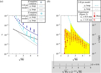
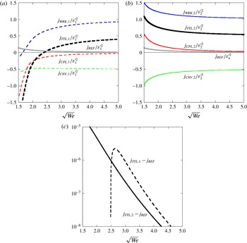
, as shown by the blue and black dashed lines in figure 4(a). As
 $\sqrt{We}$
increases, the
 ${\it\gamma}_{n}$
self-destabilising loop results in a smaller
 ${\it\varepsilon}_{n}^{\prime }$
value. However, the phase matching condition
 $$\begin{eqnarray}\displaystyle {\it\theta}_{n} & = & \displaystyle \left({\it\alpha}-{\it\gamma}_{n}\right){\displaystyle \frac{1}{{\it\beta}}}\ln {\displaystyle \frac{Y_{B}}{{\it\varepsilon}_{n}^{\prime }}}-\tan ^{-1}\left({\displaystyle \frac{{\it\alpha}}{{\it\beta}}}-{\displaystyle \frac{{\it\alpha}^{2}+{\it\beta}^{2}}{{\it\gamma}_{n}{\it\beta}}}\right)\nonumber\\ \displaystyle & & \displaystyle +\,{\it\theta}_{n}+\tan ^{-1}{\displaystyle \frac{\text{Im}\left(R_{n}\right)}{\text{Re}\left(R_{n}\right)}}+{\rm\pi}-2{\rm\pi}m\quad (m=0,\pm 1,\pm 2,\ldots )\end{eqnarray}$$
is satisfied by any value of
 ${\it\theta}_{n}$
. Nevertheless, it is only satisfied at discrete values of
 $\sqrt{We}$
corresponding to certain values of the integer
 $m$
. Substituting into (4.32) the
 ${\it\varepsilon}_{n}^{\prime }$
value determined from (4.31), we can determine the value of
 $\sqrt{We}$
which satisfies (4.32) for a certain value of the integer
 $m$
. This calculation results in a series of
 $\sqrt{We}$
values,
 $\sqrt{We}=1.65,1.84,1.97,\ldots$
for the
 ${\it\gamma}_{1}$
curve and
 $\sqrt{We}=1.53,1.58,1.63,\ldots$
for the
 ${\it\gamma}_{2}$
curve. The intervals between these discrete points are reduced as
 $\sqrt{We}$
increases. In total, there are approximately 90 and 140 points until the value of
 $\sqrt{We}=5$
is attained. On each curve segment between the neighbouring discrete points, the
 ${\it\gamma}_{n}$
self-destabilising loop is realisable, with the breakup location temporally fluctuating about the
 $L_{B}$
value of the
 ${\it\gamma}_{n}$
curve.
Predicted initial amplitudes of self-destabilising PR unstable waves in comparison with the microgravity experiment results: (a) calculated results; (b) comparison of results with those elicited in the microgravity experiments. The grey part denotes the scales for solutions in the case of an orifice jet contraction ratio of 0.9, as subsequently discussed in the text.

4.3.4 2-D jet model case
The 1-D jet model is valid for rather long wavelengths. As the jet speed increases, the neutral waves shorten their wavelengths, and the 1-D jet model is not appropriate for their description. Therefore, we considered the use of the 2-D jet model to describe the neutral waves. The forcing term in (4.5) expresses the contribution from the long waves, which should be unchanged for the 2-D jet model (note that the 2-D model reduces to the 1-D model for long waves.). Therefore, we can derive more accurate neutral waves by simply replacing the 1-D model dispersion relation with the 2-D model dispersion relation
 $$\begin{eqnarray}D\left(k,{\it\omega}\right)=\left(k-{\it\omega}\right)^{2}-\left|k\right|\left(k^{2}-1\right)/We=0\end{eqnarray}$$
in (4.16). In figure 4(a), the
 ${\it\gamma}_{n}$
loops derived in this way are represented with aqua and grey dashed lines. As anticipated, they approach each other at large
 $\sqrt{We}$
values.
4.3.5 Complete solution
The simultaneous equations (4.27)–(4.30) were solved for the 1-D and 2-D jet models. The dependence of
 ${\it\varepsilon}$
on
 $\sqrt{We}$
is shown in figure 4(a). At each value of
 $\sqrt{We}$
, there are multiple discrete solutions for
 ${\it\varepsilon}$
(and hence
 $L_{B}$
), each of which is plotted with a circle in blue colour (1-D jet model) and aqua colour (2-D jet model). As
 $\sqrt{We}$
increases, the number of the discrete solutions increases. It can be noted that there is a single solution at
 $\sqrt{We}<2.3$
. In the
 ${\it\gamma}_{1}$
and
 ${\it\gamma}_{2}$
self-destabilising loop calculations, the two loops are assumed to be formed independently. Since a larger
 ${\it\varepsilon}$
value results in a shorter breakup length, the
 ${\it\gamma}_{1}$
self-destabilising loop tends to be realised dominantly. The complete solutions, which account for both elementary self-destabilising loop contributions, are naturally located above the
 ${\it\gamma}_{1}$
self-destabilising loop expressed by the blue and aqua dashed lines.
5 Comparison with the microgravity experimental results and discussion
5.1 Dependence of experimentally determined
${\it\varepsilon}$
on
$\sqrt{We}$


Figure 5 shows typical images taken with a high-speed CCD camera (Fotron Co., FASTCAM-MAX) during a 4 s experimental run of
 $\sqrt{We}=1.6$
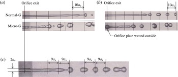
and 2 in parabolic flights. For reference, figure 5(a) contains the corresponding laboratory experimental results and a case when the outer orifice exit remains wetted by the issued water during the experimental run. Figure 5(b) clearly demonstrates the excitation of the most unstable PR wave elements, which tend to disintegrate the jet at the shortest distance for
 $\sqrt{We}=2$
.
It is difficult to observe the very small amplitude of local surface deformation developing along the long jet. Therefore, our strategy was to extract the jet deformation dynamics from the jet breakup location data. Our compact microgravity experimental set-up photographs the entire water jet disintegrating into droplets at a resolution of
 $1024\times 240~\text{pixels}$
, which could resolve the size of the orifice radius using approximately 10 pixels. The distance
 $X^{\prime }$
from the orifice exit, where the PR unstable wave amplitude exceeds the resolution of 0.1, is estimated from the relation
 $0.1=\text{e}^{{\it\beta}(X-L_{B})}={\it\varepsilon}^{(1-X^{\prime }/L_{B})}$
as
 $X^{\prime }/L_{B}=1-\ln 0.1/\ln {\it\varepsilon}=0.667$
for
 ${\it\varepsilon}=10^{-3}$
and 0.750 for
 ${\it\varepsilon}=10^{-4}$
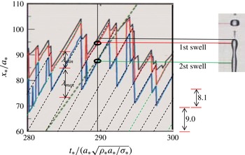
. This implies that only the surface deformation of at most two PR unstable wave elements near the breakup location can be resolved satisfactorily, although we can recognise some further upstream surface deformation by virtue of the brightness variation on the jet image, which is caused by the refraction of backlight rays passing through the jet. Nevertheless, the image resolution is fine enough to measure the instantaneous jet tip distance from the orifice exit. The black solid line of figure 6 shows the tip location history for the case of
 $a_{\ast }=1~\text{mm}$
and
 $\sqrt{We}=4$
. This was obtained from each image by scanning the brightness variation along the jet centreline from the continuous jet side, and identifying the instantaneous tip location with an approximate resolution of 0.1. This resolution is very small compared to the breakup length
 $L_{B}\sim 100$
. The jet tip location history has a saw-tooth-like shape. The upstream location
 $x=L_{n}\;(n=1,2,\ldots )$
of each discontinuous drop indicates the location where the jet disintegrates. By generating the frequency diagram of
 $L_{n}$
measured for the last 2 s of the experimental run, the average breakup length
 $L_{B}$
was calculated.
Examples of orifice water jet images obtained in the microgravity experiments. For comparison, the laboratory experimental results at a low-jet-issue speed are also shown. (a,b)
 $\sqrt{We}=1.6$
, (c)
 $\sqrt{We}=2.0$
; (a)
 $a_{\ast }=1.0~\text{mm}$
, (b)
 $a_{\ast }=0.4~\text{mm}$
.

Example of jet tip location history (thick black solid line) for
 $\sqrt{We}=4$
and
 $a_{\ast }=1~\text{mm}$
. The red and blue lines (and their extended straight dashed black lines) represent the histories of the first and second swell locations defined by the image on the right. These lines can be used to identify each jet-disintegration location, as well as the wavelength
 ${\it\lambda}$
and phase velocity of the PR unstable wave element involved in the jet disintegration. The slope of the green dashed line represents the jet-issue speed.

The jet deformation observed in the microgravity experiments was not completely periodic for any
 $\sqrt{We}$
under consideration. This feature is similar in all laboratory experiments reported in the literature, in which the ‘average’ breakup length is used to characterise the jet-disintegration location. In figure 6, the first and second swell locations (counting from the jet tip) are also indicated. These move linearly with time, as shown by the red and blue lines, respectively. Their jumps occur when an overlapping tip contraction dispersive wave eliminates the first swell temporally. It is noted that the black dashed lines tangent to the loci are all parallel. This indicates that each PR unstable wave element moves at the same speed as the steady jet speed. Each PR unstable wave element approaching the jet tip has a wavelength fluctuating about a certain value close to the most unstable wavelength
 $2{\rm\pi}/{\it\alpha}$
. The longest and shortest element lengths in figure 6 are
 ${\it\lambda}_{max}=11.7=1.44(2{\rm\pi}/{\it\alpha})$
and
 ${\it\lambda}_{min}=6.2=0.765(2{\rm\pi}/{\it\alpha})$
, which have the growth rates 0.853
 ${\it\beta}$
and 0.705
 ${\it\beta}$
, respectively. The breakup location fluctuates about the average breakup length
 $L_{B}$
.
Hence, when the experimentally observed jet surface deformation in the linear region is described in terms of the linear stability analysis solutions, the frequency must have a distribution, among which the frequency producing the most unstable wave determines the ‘average’ breakup length. This conventionally believed scenario is justified when the mechanism by which the average breakup length is determined as a function of jet-issue speed is stable against possible perturbations, as discussed at the end of this section.
Consistent with the breakup condition explained in § 4.3.1, the steady jet radius appears to be uniform over the entire continuous jet portion. Therefore, using the
 ${\it\beta}$
value given by (3.4b
), the breakup condition
 $Y_{B}=1$
was applied to evaluate the initial PR unstable wave amplitude
 ${\it\varepsilon}=\text{e}^{-{\it\beta}L_{B}}$
for the experimentally measured average breakup length
 $L_{B}$
(figure 1). The calculated
 ${\it\varepsilon}$
values are plotted with red open circles (
 $a_{\ast }=0.4~\text{mm}$
) and squares (
 $a_{\ast }=1~\text{mm}$
) in figure 4(b). They should be compared with the aqua and grey dashed lines based on the 2-D jet model.
5.2 Findings from experimental comparisons
Basically, our self-destabilising concept claims that the formation of a PR unstable wave element responsible for each jet disintegration depends on the history of various waves produced in the jet in the past. Therefore, the fluctuation of the instantaneous breakup location is an inherent character of the self-destabilising mechanism. To interpret figure 4(b), it is important to note that the
 ${\it\omega}={\it\alpha}$
periodicity of the jet deformation, assumed in the weakly nonlinear analysis, is degraded in the experiments because of the distributed frequency. Unlike each PR unstable wave element responsible for the instantaneous jet disintegrations in figure 6, the most unstable PR wave element used in the calculation of the experimental plots in figure 4(b) is a hypothetical PR unstable wave element. The jet-disintegration location caused by a PR unstable wave element depends on both its initial amplitude and the growth rate. As seen in figure 6, the measured average breakup length includes contributions from the instantaneous breakup lengths caused by the PR unstable wave elements with smaller growth rates (different frequency). Therefore, the real PR unstable wave element resulting in the instantaneous breakup length
 $L_{B}$
should have a smaller growth rate equal to
 $(1-{\it\psi}){\it\beta}$
. Its initial amplitude
 ${\it\varepsilon}_{{\it\psi}}=\text{e}^{-(1-{\it\psi}){\it\beta}L_{B}}$
is correlated with
 ${\it\varepsilon}$
as
 ${\it\varepsilon}_{{\it\psi}}={\it\varepsilon}^{1-{\it\psi}}$
. Consider, for example, the case of figure 6. If we use the maximum
 ${\it\psi}$
value, i.e.
 ${\it\psi}=1-0.705=0.295$
,
 ${\it\varepsilon}\sim 10^{-4}$
leads to
 ${\it\varepsilon}_{{\it\psi}}\sim 0.00151$
, which is slightly larger than the upper limit of the aqua circle plots in figure 4(a). At half its maximum value, namely
 ${\it\psi}=0.1475$
,
 ${\it\varepsilon}_{{\it\psi}}\sim 0.000389$
, which is on the aqua dashed line. Therefore, we may expect that the real initial PR unstable wave amplitude is in fairly good agreement with the theoretical prediction, although it is not easy to develop an image processing algorithm to do such
 ${\it\psi}$
correction statistically. The growth rate with small
 ${\it\psi}$
values is considered to have a similar
 $\sqrt{We}$
dependence as that of the most unstable wave. In addition, all quantities derived from the weakly nonlinear analyses are regular functions of
 ${\it\omega}={\it\alpha}$
. Therefore, for our purpose of examining the dependence of
 ${\it\varepsilon}$
on
 $\sqrt{We}$
, the real PR unstable wave element responsible for the average breakup length may be represented by the most unstable PR wave. We thus compare the experimental plots with the theoretical predictions.
The experimental plots in figure 4(b) are all below the aqua circles in figure 4(a), and appear to be along the grey dashed line (2-D
 ${\it\gamma}_{2}$
loop) at
 $1.5<\sqrt{We}<2.3$
and the aqua dashed line (2-D
 ${\it\gamma}_{1}$
loop) at
 $3<\sqrt{We}<4.5$
. It would be safe to say that the experimental plots in figure 4(b) are consistent in behaviour with the theoretical plots in figure 4(a) at
 $2.5<\sqrt{We}<4.5$
. It is found that the jet disintegration is dominated by the 2-D
 ${\it\gamma}_{1}$
self-destabilising loop. A longer jet is necessary for the
 ${\it\gamma}_{1}$
neutral wave to be established in the near-orifice region. This is because, as seen in appendix B, the
 ${\it\gamma}_{1}$
neutral wave is established downstream of a temporally stationary wave element of each upstream propagating dispersive wave, while the
 ${\it\gamma}_{2}$
neutral wave is produced upstream. A transitional behaviour of experimental plots, observed near
 $\sqrt{We}=2.5$
, is explained as follows.
Upstream energy flux
 $j_{TTL,n}$
of the
 ${\it\gamma}_{n}$
neutral wave, which consists of a convective contribution
 $j_{CNV,n}$
, a capillary wave contribution
 $j_{CPL,n}$
and a work contribution
 $j_{WRK,n}$
;
 $j_{REF}$
denotes the least energy flux necessary to generate the most unstable wave element at the orifice exit. (a) Upstream energy flux of the
 ${\it\gamma}_{1}$
neutral wave. (b) Upstream energy flux of the
 ${\it\gamma}_{2}$
neutral wave. (c) Excess upstream energy flux of the
 ${\it\gamma}_{n}$
self-destabilising loop. The grey line in (a) and (b) represents
 $j_{REF}/{\it\varepsilon}_{1}^{\prime 2}$
and
 $j_{REF}/{\it\varepsilon}_{2}^{\prime 2}$
, respectively.

Equations (3.11)–(3.13) (thereby, all self-destabilising curves in figure 4
a) predict the presence of the PR unstable wave involved. Additional energetic (causal) consideration is necessary to examine whether the predicted PR unstable wave can be formed by the reflection of the neutral waves at the orifice exit. The basic jet is the uniform liquid jet flow, and has a constant downstream energy flux
 $j_{0\ast }=(0.5{\it\rho}_{\ast }U_{\ast }^{2}+{\it\sigma}_{\ast }/a_{\ast })U_{\ast }$
. Consider a basic jet element which has the same length as the PR unstable wavelength
 ${\it\lambda}_{\ast }=2{\rm\pi}/{\it\alpha}_{\ast }$
. This element is issued during each and every time period equal to
 ${\it\lambda}_{\ast }/U_{\ast }$
. If its surface is deformed to the sinusoidal shape
 ${\it\varepsilon}_{\ast }\cos ({\it\alpha}_{\ast }x_{\ast })$
with the element volume and kinetic energy being conserved within the element, the deformed jet element gains the surface energy
 ${\it\sigma}_{\ast }2{\rm\pi}^{3}a_{\ast }{\it\varepsilon}_{\ast }^{2}/{\it\lambda}_{\ast }$
. In the conventional theory, this energy is assumed to be supplied from the issuing liquid, so that the time-averaged downstream energy flux of the disturbed jet flow should be positive at the orifice exit. In our self-destabilising mechanism, this surface energy should be supplied from downstream as the upstream energy transfer rate
 $J_{REF\ast }=({\it\sigma}_{\ast }2{\rm\pi}^{3}a_{\ast }{\it\varepsilon}_{\ast }^{2}/{\it\lambda}_{\ast })/({\it\lambda}_{\ast }/U_{\ast })$
, so that the same unstable wave element might be produced periodically, immediately downstream of the orifice exit. In appendix C, the upstream energy fluxes of the 2-D
 ${\it\gamma}_{n}$
neutral waves are calculated. Figure 7(a,b) show the dimensionless upstream energy fluxes of the
 ${\it\gamma}_{1}$
and
 ${\it\gamma}_{2}$
neutral waves, respectively. For the
 ${\it\gamma}_{1}$
and
 ${\it\gamma}_{2}$
self-destabilising loops to be established, their upstream energy fluxes should be at least greater than
 $j_{REF}=J_{REF\ast }/({\rm\pi}a_{\ast }^{2}{\it\rho}_{\ast }U_{\ast }^{3})=({\it\alpha}{\it\varepsilon})^{2}/(2We)$
. The excess energy (
 $j_{TTL,n}-j_{REF}$
) is partially used to produce higher-frequency disturbances superimposed on the jet, which are ignored in the present study because they do not contribute to our self-destabilising mechanism. Figure 7(a,b) indicates that the
 ${\it\gamma}_{2}$
self-destabilising loop may operate over the entire
 $\sqrt{We}$
range, whereas the
 ${\it\gamma}_{1}$
self-destabilising loop cannot be established at
 $\sqrt{We}>2.5$
. For the
 $\sqrt{We}$
range where the two self-destabilising loops may operate, we can see which one is dominant by comparing the values of
 $j_{TTL,1}-j_{REF}$
and
 $j_{TTL,2}-j_{REF}$
in figure 7(c). The complete solution (plotted using circles in figure 4
a), which is based on the continuity equation and momentum equation only, cannot describe such a switching behaviour as highlighted in yellow in figure 4(b). It yields a larger
 ${\it\varepsilon}$
value at
 $\sqrt{We}<2.5$
, which cannot be realised physically. It is reasonable to consider that transitions between the dominant
 ${\it\gamma}_{1}$
and
 ${\it\gamma}_{2}$
self-destabilising loops take place at values close to
 $\sqrt{We}=2.5$
. These transitions occur in a form such that breakups owing to the
 ${\it\gamma}_{1}$
and
 ${\it\gamma}_{2}$
self-destabilising loops are realised intermittently, whereby the breakup length fluctuates relatively widely, as seen from the error bar lengths. At
 $\sqrt{We}<2.5$
, the
 ${\it\gamma}_{2}$
self-destabilising loop becomes dominant, consistent with the experimental result. The same energy flux calculations were conducted for the 1-D jet model as well, and indicate that the upstream energy flux of the
 ${\it\gamma}_{1}$
neutral wave becomes negative at
 $\sqrt{We}<1.8$
. Thus, an accurate neutral wave prediction is important for considering the self-destabilising loop.
5.3 Orifice jet contraction
Water separated from the entrance edge of the orifice hole forms a uniform jet of smaller dimensionless radius
 $\hat{a}$
(contraction ratio). The dimensionless uniform jet speed
 $\hat{U}$
is determined from the continuity equation
 $\hat{U} \hat{a}^{2}=1$
, and its Weber number based on the contracted uniform jet radius is given by
 $\hat{We}=We/\hat{a}^{3}$
. The length of the contracting portion is comparable to the orifice radius, and is negligible compared to the breakup length. The contraction ratio
 $\hat{a}$
may decrease from unity as the orifice radius
 $a_{\ast }$
and the jet-issue speed
 $U_{\ast }$
are increased. In the microgravity experiments, the contraction ratio was larger than approximately 0.9, even for the largest jet-issue speed (
 $\sqrt{We}=4.5$
) from the
 $a_{\ast }=1~\text{mm}$
orifice. In fact, in figure 6, for
 $\sqrt{We}=4$
and
 $a_{\ast }=1~\text{mm}$
, the thick green dashed straight line expresses the path of a particle moving with the jet-issue speed. Since the thin black dashed straight lines are 1.20 times larger than the jet-issue speed, the experimentally realised jet is found to contract by a ratio of 0.914.
It is difficult to conduct a 2-D global analysis that includes the contracting portion. However, the jet contraction effect on
 ${\it\varepsilon}_{n}^{\prime }$
can be estimated using the present analysis as follows. The breakup length should be mainly determined by the PR unstable wave which minimises the uniform jet portion length. Since this wave has a considerably longer wavelength than the contracting portion, it is not significantly influenced by the contracting portion. Therefore, we may consider the PR unstable wave growth of the initial amplitude
 $\hat{{\it\varepsilon}}_{n}^{\prime }={\it\varepsilon}_{n}^{\prime }/\hat{a}$
for the uniform jet of radius
 $\hat{a}$
, extended to
 $x=0$
, and apply the amplitude matching condition (4.31). Since the short neutral waves are dispersed and generate other-frequency waves when entering the contracting portion, a necessary modification requires that the initial PR unstable wave amplitude in (4.31) must be replaced by
 $\hat{{\it\varepsilon}}_{n}^{\prime }/{\it\phi}$
. In this case,
 ${\it\phi}\leqslant 1$
denotes the effectiveness of the dispersed wave for the reproduction of the PR unstable wave. As a result, the dependences of
 ${\it\varepsilon}_{n}^{\prime }/({\it\phi}\hat{a})$
on
 $\sqrt{\hat{We}}$
become the same as the two dashed curves in figure 4(b), and the jet contraction reduces
 ${\it\varepsilon}_{n}^{\prime }$
by
 ${\it\phi}\hat{a}$
, thereby shifting the two dashed curves slightly downwards at large
 $\sqrt{We}$
.
On the other hand, for the experimental plots, the breakup condition
 $Y_{B}=1$
must be interpreted as the condition
 $\hat{{\it\varepsilon}}_{n}^{\prime }\text{e}^{\hat{{\it\beta}}(L_{B}/\hat{a})}=1$
for each measured
 $L_{B}$
, where
 $\hat{{\it\beta}}$
is equal to the value of
 ${\it\beta}(\sqrt{We})$
evaluated at
 $\sqrt{We}=\sqrt{\hat{We}}$
. Therefore, we have the relation
 $$\begin{eqnarray}{\it\varepsilon}_{n}^{\prime }=\hat{a}\exp \left(-\!\left.{\it\beta}\right|_{\sqrt{\hat{We}}}\frac{L_{B}}{\hat{a}}\right)=\hat{a}\exp \left(gL_{B}\right){\it\varepsilon}_{exp}\end{eqnarray}$$
where
 $$\begin{eqnarray}{\it\varepsilon}_{exp}=\exp \left(\left.-{\it\beta}\right|_{\sqrt{We}}L_{B}\right),\quad g=\left.{\it\beta}\right|_{\sqrt{We}}\left\{1-{\displaystyle \frac{{\it\beta}|_{\sqrt{\hat{We}}}}{\left.{\it\beta}\right|_{\sqrt{We}}}}{\displaystyle \frac{1}{\tilde{a}}}\right\}.\end{eqnarray}$$
For example, at
 $\sqrt{We}=4$
,
 $L_{B}=92.9$
and
 $g$
takes a value of 0.0054 for
 $\tilde{a}=0.9$
, which leads to the multiplying factor
 $\hat{a}\exp (gL_{B})=0.9\times 1.66=1.50$
.
The two modifications above allow the experimental plot and the blue dashed curve to come closer in figure 4(b) at larger
 $\sqrt{We}$
.
When the outer orifice plate is wetted by the liquid jet base, a similar consideration can account for the wetting liquid portion. Since the neutral waves collide with the orifice plate surface,
 ${\it\phi}$
may take a considerably smaller value. Therefore, the resulting PR unstable wave may have a considerably smaller amplitude, as seen in figure 4(b).
5.4 Stability of the self-destabilising loop
Importantly, both the amplitude matching conditions (4.29) and (4.31) for the overall and elementary self-destabilising loops tend to stably determine the initial PR unstable wave amplitudes and, consequently, the breakup length
 $L_{B}$
as a function of
 $\sqrt{We}$
. To explain this, we let
 $X_{max}={\it\phi}L_{B}\;(0<{\it\phi}<1)$
. Equations (4.29) and (4.31) can then be respectively rewritten as
 $$\begin{eqnarray}\displaystyle R_{1}{\it\varepsilon}^{3}\text{e}^{3{\it\beta}X_{max}}=R_{1}{\it\varepsilon}^{3}\text{e}^{3{\it\beta}{\it\phi}L_{B}}=R_{1}[({\it\varepsilon}\text{e}^{{\it\beta}L_{B}})^{{\it\phi}}{\it\varepsilon}^{1-{\it\phi}}]^{3}=R_{1}Y_{B}^{3{\it\phi}}{\it\varepsilon}^{3(1-{\it\phi})}=K_{1}{\it\varepsilon}, & & \displaystyle\end{eqnarray}$$
 $$\begin{eqnarray}\displaystyle R_{n}{\it\varepsilon}_{n}^{\prime 3}\text{e}^{3{\it\beta}X_{max}}=R_{n}{\it\varepsilon}_{n}^{\prime 3}\text{e}^{3{\it\beta}{\it\phi}L_{B}}=R_{n}[({\it\varepsilon}_{n}^{\prime }\text{e}^{{\it\beta}L_{B}})^{{\it\phi}}{\it\varepsilon}_{n}^{\prime 1-{\it\phi}}]^{3}=R_{n}Y_{B}^{3{\it\phi}}{\it\varepsilon}_{n}^{\prime 3(1-{\it\phi})}=K_{n}^{\prime }{\it\varepsilon}_{n}^{\prime }. & & \displaystyle\end{eqnarray}$$
Therefore, if
 $3(1-{\it\phi})<1$
or
 $2/3<{\it\phi}<1$
, the
 ${\it\varepsilon}$
and
 ${\it\varepsilon}_{n}^{\prime }$
values determined from (5.3) are stable for given values of
 $\sqrt{We}$
and
 $Y_{B}$
, as illustrated in figure 8. To treat all self-destabilising loops with the single figure 8, the function
 $K_{1}$
, which varies with
 ${\it\varepsilon}$
periodically and with a small amplitude about
 $K_{1,mean}$
(see (4.26)), is represented by the constant value
 $K_{1,mean}$
. Equation (5.3) indicates that a neutral wave, produced by the nonlinear growth of a PR unstable wave with an initial amplitude
 ${\it\varepsilon}={\it\varepsilon}^{(m)}(m=1,2,\ldots )$
on the left-hand side of (5.3), reproduces a new synchronised PR unstable wave with an initial amplitude
 ${\it\varepsilon}={\it\varepsilon}^{(m+1)}$
, as described by the right-hand side of (5.3). An iteration of this process allows
 ${\it\varepsilon}^{(m)}$
to converge to the solution
 ${\it\varepsilon}$
in (5.3) for
 $2/3<{\it\phi}<1$
, even if the periodic variation of
 $K_{1}$
is taken into account. In particular, the curves in figure 4, for which
 ${\it\varepsilon}$
is determined in the limit of
 ${\it\phi}\rightarrow 1$
, are stable. Thus,
 ${\it\varepsilon}$
is an eigenvalue of the dynamic system under consideration.
Stability of the self-destabilising loops. The intersection point (solid circle) of the two thick solid lines expresses the solution of
 $R_{1}Y_{B}^{3{\it\phi}}{\it\varepsilon}^{3(1-{\it\phi})}=K_{1}{\it\varepsilon}$
or
 $R_{n}Y_{B}^{3{\it\phi}}{\it\varepsilon}_{n}^{\prime 3(1-{\it\phi})}=K_{n}^{\prime }{\it\varepsilon}_{n}^{\prime }$
. A different self-destabilising loop represented by an open circle on the curved solid line tends to settle down to this point, as indicated by the two thin arrowed lines.

We have no means to directly measure the instantaneous jet-issue velocity with a high degree of accuracy. To prove that the experimentally observed PR unstable waves at
 $\sqrt{We}=4$
, for example, are not produced by an uncontrolled jet-issue velocity fluctuation of amplitude
 ${\rm\Delta}U$
, (3.10b
) requires a measurement precision of at least
 $O(10^{\text{-5}})$
. Nevertheless, it is difficult to believe that the reproducible jet disintegration is caused by a ‘noise’ possessed by the water pushed out by the piston. Instead, the noise considered in the conventional linear stability analysis may be interpreted to express the presence of the neutral wave or upstream propagating dispersive wave forming the self-destabilising loop. Then, the reason why the average breakup length is determined as a function of jet-issue speed is clarified. Even if there is a rather large amplitude of jet-issue velocity fluctuation, this does not dominate the breakup length when its frequency is not close to the most unstable PR wave frequency. Furthermore, the smallness of
 ${\it\varepsilon}$
at large
 $\sqrt{We}$
values does not affect the realisation of the self-destabilising loop. This is clear from the conventional linear stability analyses which consider an infinitesimal amplitude of noise. What is important is the presence of a certain mechanism that can produce the long-wave structure of the most unstable PR wave element.
However, it is unlikely that the self-destabilising loop explored in the present study works for high-speed jets. In fact, it is well known that the breakup length is maximised at a certain jet-issue speed (the critical point). A similar trend was observed in our laboratory orifice jet experiments at jet-issue speeds greater than
 $\sqrt{We}=4$
. The following scenarios are anticipated at higher jet-issue speeds, where
 ${\it\varepsilon}$
takes a very small value. If a larger initial PR unstable wave amplitude is excited in the near-orifice region by another self-destabilising loop associated with the injector entrance flow (Phinney & Humphries Reference Phinney and Humphries1973; McCarthy & Molloy Reference McCarthy and Molloy1974; Umemura et al.
Reference Umemura, Kawanabe, Suzuki and Osaka2011) or the surrounding gas (Weber Reference Weber1931; Sterling & Sleicher Reference Sterling and Sleicher1975; Shinjo & Umemura Reference Shinjo and Umemura2010), this self-destabilising loop dominates the jet disintegration. The effect of such a self-destabilising loop formed within an injector may be accounted for by the definition of
 ${\rm\Delta}U$
in (3.8). The value of
 ${\it\varepsilon}_{ref}/{\rm\Delta}U$
, calculated using (3.10b
), is not so sensitive to
 ${\it\omega}$
, but increases significantly with
 $\sqrt{We}$
. Therefore, a further increase in
 $\sqrt{We}$
enables the
 ${\rm\Delta}U$
effect to overwhelm the
 ${\it\varepsilon}$
value in figure 4(b), as clearly observed for nozzle jets.
6 Conclusion
We have conducted a global mode analysis to understand the instabilities observed in water jets emanating from an orifice in microgravity at jet-issue speeds ranging from
 $\sqrt{We}=\sqrt{2}$
to 4.5. The experiments exhibited a reproducible average breakup length determined as a function of the speed at which jets were issued. The initial amplitude of the PR unstable wave, calculated from the breakup length, was small. These facts suggest that the experimentally observed jet instability is excited by the dynamics of the jet itself, and not by the noise, as conventionally believed.
The continuous jet region can be divided into three regions according to the stages of PR unstable wave growth: (1) the linear region,
 $0<x<X$
, where all disturbance wave amplitudes are small and the conventional linear stability analysis is applicable; (2) the weakly nonlinear region,
 $X<x<X_{max}$
, where the amplified PR unstable wave exhibits nonlinear evolution and radiates the upstream propagating dispersive waves; and (3) the highly nonlinear breakup region,
 $X_{max}<x<L_{B}$
, where the PR surface deformation amplitude is saturated, and the surface energy released at the pinching portion is consumed by the higher modes in order to break the jet.
When a PR unstable wave is predicted by the linear stability analysis, there also exists an upstream propagating neutral wave among the wave modes excitable in the linear region. The regular perturbation expansion equation system, with respect to an unknown initial PR unstable wave amplitude to the orifice radius ratio,
 ${\it\varepsilon}$
, was solved to third order in order to determine the
 ${\it\varepsilon}$
value. The solutions successfully capture the process wherein the nonlinear PR unstable wave growth produces an upstream propagating neutral wave appearing in the linear region, transfers energy upstream to the orifice exit, and excites a new PR unstable wave on the newly issued liquid. The PR unstable wave can continue to be reproduced through this self-destabilising loop. The initial amplitude
 ${\it\varepsilon}$
of a newly produced PR unstable wave is determined from the amplitude of the upstream propagating neutral wave. For jets issued at high speeds, the long jet allows the radiated upstream propagating dispersive waves to integrate to a monochromatic capillary wave, so that the jet disintegration takes place periodically to a good degree of approximation. The predicted
 ${\it\varepsilon}$
value was consistent with the experimental microgravity results. On the other hand, for a short jet issued at low speeds, the self-destabilising loop must comprise individual upstream propagating dispersive waves, and jet disintegration occurs in conjunction with end-pinching. As a result, the jet breakup location fluctuates considerably about a stable average breakup location.
Acknowledgements
The present study was supported by the ‘Ground-based Research Programme for Space Utilisation’ promoted by the Japan Space Forum.
Appendix A. Regular perturbation expansion equations and their particular solutions
 $$\begin{eqnarray}F_{2}=-v_{1}{\displaystyle \frac{\partial {\it\delta}_{1}}{\partial x}}-{\displaystyle \frac{1}{2}}{\it\delta}_{1}{\displaystyle \frac{\partial v_{1}}{\partial x}},\quad G_{2}=-v_{1}{\displaystyle \frac{\partial v_{1}}{\partial x}}-{\displaystyle \frac{1}{We}}2{\it\delta}_{1}{\displaystyle \frac{\partial {\it\delta}_{1}}{\partial x}}+{\displaystyle \frac{1}{We}}{\displaystyle \frac{\partial {\it\delta}_{1}}{\partial x}}{\displaystyle \frac{\partial ^{2}{\it\delta}_{1}}{\partial x^{2}}},\end{eqnarray}$$
 $$\begin{eqnarray}F_{3}=-v_{1}{\displaystyle \frac{\partial {\it\delta}_{2}}{\partial x}}-v_{2}{\displaystyle \frac{\partial {\it\delta}_{1}}{\partial x}}-{\displaystyle \frac{1}{2}}{\it\delta}_{1}{\displaystyle \frac{\partial v_{2}}{\partial x}}-{\displaystyle \frac{1}{2}}{\it\delta}_{2}{\displaystyle \frac{\partial v_{1}}{\partial x}},\end{eqnarray}$$
 $$\begin{eqnarray}\displaystyle G_{3} & = & \displaystyle -v_{2}{\displaystyle \frac{\partial v_{1}}{\partial x}}-v_{1}{\displaystyle \frac{\partial v_{2}}{\partial x}}-{\displaystyle \frac{1}{We}}2{\it\delta}_{2}{\displaystyle \frac{\partial {\it\delta}_{1}}{\partial x}}-{\displaystyle \frac{1}{We}}2{\it\delta}_{1}{\displaystyle \frac{\partial {\it\delta}_{2}}{\partial x}}+{\displaystyle \frac{1}{We}}3{\it\delta}_{1}^{2}{\displaystyle \frac{\partial {\it\delta}_{1}}{\partial x}}\nonumber\\ \displaystyle & & \displaystyle -\,{\displaystyle \frac{1}{We}}{\displaystyle \frac{1}{2}}\left({\displaystyle \frac{\partial {\it\delta}_{1}}{\partial x}}\right)^{3}-{\displaystyle \frac{1}{We}}{\it\delta}_{1}{\displaystyle \frac{\partial {\it\delta}_{1}}{\partial x}}{\displaystyle \frac{\partial ^{2}{\it\delta}_{1}}{\partial x^{2}}}+{\displaystyle \frac{1}{We}}{\displaystyle \frac{\partial {\it\delta}_{2}}{\partial x}}{\displaystyle \frac{\partial ^{2}{\it\delta}_{1}}{\partial x^{2}}}\nonumber\\ \displaystyle & & \displaystyle +\,{\displaystyle \frac{1}{We}}{\displaystyle \frac{\partial {\it\delta}_{1}}{\partial x}}{\displaystyle \frac{\partial ^{2}{\it\delta}_{2}}{\partial x^{2}}}-{\displaystyle \frac{1}{We}}{\displaystyle \frac{3}{2}}\left({\displaystyle \frac{\partial {\it\delta}_{1}}{\partial x}}\right)^{2}{\displaystyle \frac{\partial ^{3}{\it\delta}_{1}}{\partial x^{3}}}-{\displaystyle \frac{1}{We}}3{\displaystyle \frac{\partial {\it\delta}_{1}}{\partial x}}\left({\displaystyle \frac{\partial ^{2}{\it\delta}_{1}}{\partial x^{2}}}\right)^{2}.\end{eqnarray}$$
To solve the perturbation equations (2.6) and (2.7), it is convenient to use complex expressions by putting
 ${\it\zeta}={\it\alpha}-\text{i}{\it\beta}$
. The second-order particular solutions are given by
 $$\begin{eqnarray}{\it\delta}_{2}={\it\delta}_{2,2}+{\it\delta}_{2,0},\quad {\it\delta}_{2,2}=A_{2}\text{e}^{\text{i}2{\it\zeta}x-\text{i}2{\it\omega}t}\text{e}^{\text{i}2{\it\Theta}}+\text{c.c.},\quad {\it\delta}_{20}=A_{0}\text{e}^{\text{i}({\it\zeta}-\bar{{\it\zeta}})x},\end{eqnarray}$$
 $$\begin{eqnarray}v_{2}=v_{2,2}+v_{2,0},\quad v_{2,2}=B_{2}\text{e}^{\text{i}2{\it\zeta}x-\text{i}2{\it\omega}t}\text{e}^{\text{i}2{\it\Theta}}+\text{c.c.},\quad v_{2,0}=B_{0}\text{e}^{\text{i}({\it\zeta}-\bar{{\it\zeta}})x},\end{eqnarray}$$
where
 $$\begin{eqnarray}A_{2}=\left({\displaystyle \frac{1}{2{\it\zeta}^{2}}}-1\right)A^{2},\quad B_{2}=({\it\omega}-{\it\zeta}){\displaystyle \frac{1-5{\it\zeta}^{2}}{{\it\zeta}^{3}}}A^{2},\end{eqnarray}$$
 $$\begin{eqnarray}A_{0}={\displaystyle \frac{-{\displaystyle \frac{1}{({\it\zeta}-\bar{{\it\zeta}})}}\left[({\it\zeta}A\bar{B}-\bar{{\it\zeta}}\bar{A}B)-{\displaystyle \frac{1}{2}}(\bar{{\it\zeta}}A\bar{B}-{\it\zeta}\bar{A}B)\right]+{\displaystyle \frac{1}{2}}B\bar{B}-{\displaystyle \frac{1}{We}}\left({\displaystyle \frac{1}{2}}{\it\zeta}\bar{{\it\zeta}}-1\right)A\bar{A}}{1+{\displaystyle \frac{1}{2We}}\left\{1-({\it\zeta}-\bar{{\it\zeta}})^{2}\right\}}},\end{eqnarray}$$
 $$\begin{eqnarray}B_{0}={\displaystyle \frac{-{\displaystyle \frac{1}{We}}\left\{1-({\it\zeta}-\bar{{\it\zeta}})^{2}\right\}{\displaystyle \frac{1}{({\it\zeta}-\bar{{\it\zeta}})}}\left[({\it\zeta}A\bar{B}-\bar{{\it\zeta}}\bar{A}B)-{\displaystyle \frac{1}{2}}(\bar{{\it\zeta}}A\bar{B}-{\it\zeta}\bar{A}B)\right]-B\bar{B}+{\displaystyle \frac{1}{We}}\left({\it\zeta}\bar{{\it\zeta}}-2\right)A\bar{A}}{1+{\displaystyle \frac{1}{2We}}\left\{1-({\it\zeta}-\bar{{\it\zeta}})^{2}\right\}}}.\end{eqnarray}$$
Use is made of (3.2) and (3.3) to derive the final expressions for
 $A_{2}$
and
 $B_{2}$
.
The third-order equations for the solutions with the same temporal variation as the PR unstable wave are expressed as
 $$\begin{eqnarray}{\displaystyle \frac{\partial {\it\delta}_{3}}{\partial t}}+{\displaystyle \frac{\partial {\it\delta}_{3}}{\partial x}}+{\displaystyle \frac{1}{2}}{\displaystyle \frac{\partial v_{3}}{\partial x}}=F_{3}=\text{i}S_{{\it\delta}}\text{e}^{\text{i}\left(2{\it\zeta}-\bar{{\it\zeta}}\right)x-\text{i}{\it\omega}t-\text{i}{\it\Theta}}+\text{c.c.}\end{eqnarray}$$
with
 $$\begin{eqnarray}S_{{\it\delta}}=-\!\left({\textstyle \frac{3}{2}}{\it\zeta}-\bar{{\it\zeta}}\right)\left(A_{0}B+AB_{0}\right)-\left(2{\it\zeta}-{\textstyle \frac{1}{2}}\bar{{\it\zeta}}\right)A_{2}\bar{B}-\left({\it\zeta}-\bar{{\it\zeta}}\right)\bar{A}B_{2}\end{eqnarray}$$
and
 $$\begin{eqnarray}{\displaystyle \frac{\partial v_{3}}{\partial t}}+{\displaystyle \frac{\partial v_{3}}{\partial x}}-{\displaystyle \frac{1}{We}}\left({\displaystyle \frac{\partial {\it\delta}_{3}}{\partial x}}+{\displaystyle \frac{\partial ^{3}{\it\delta}_{3}}{\partial x^{3}}}\right)=G_{3}=\text{i}S_{u}\text{e}^{\text{i}(2{\it\zeta}-\bar{{\it\zeta}})x-\text{i}{\it\omega}t-\text{i}{\it\Theta}}+\text{c.c.}\end{eqnarray}$$
with
 $$\begin{eqnarray}\displaystyle S_{u} & = & \displaystyle \bar{{\it\zeta}}\bar{B}B_{2}-{\it\zeta}B_{0}B-2{\it\zeta}\bar{B}B_{2}-({\it\zeta}-\bar{{\it\zeta}})B_{0}B\nonumber\\ \displaystyle & & \displaystyle \begin{array}{@{}l@{}}+\,{\displaystyle \frac{1}{We}}\left\{-2{\it\zeta}\bar{k}^{2}\bar{A}A_{2}-({\it\zeta}-\bar{{\it\zeta}})k^{2}A_{0}A+4\bar{{\it\zeta}}{\it\zeta}^{2}\bar{A}A_{2}-({\it\zeta}-\bar{{\it\zeta}})^{2}{\it\zeta}A_{0}A\right.\\ -\,\text{i}3{\it\zeta}^{3}\bar{{\it\zeta}}A^{2}\bar{A}+\text{i}{\textstyle \frac{3}{2}}{\it\zeta}^{2}\bar{{\it\zeta}}^{2}A^{2}\bar{A}-6{\it\zeta}^{3}\bar{{\it\zeta}}^{2}A^{2}\bar{A}+3{\it\zeta}^{4}\bar{{\it\zeta}}A^{2}\bar{A}\\ +\,6{\it\zeta}A^{2}\bar{A}-3\bar{{\it\zeta}}A^{2}\bar{A}-\,{\textstyle \frac{3}{2}}{\it\zeta}^{2}\bar{{\it\zeta}}A^{2}\bar{A}+{\it\zeta}^{2}({\it\zeta}-\bar{{\it\zeta}})A^{2}\bar{A}+{\it\zeta}\bar{{\it\zeta}}^{2}A^{2}\bar{A}\\ +\left.2\bar{{\it\zeta}}\bar{A}A_{2}-2{\it\zeta}A_{0}A-4{\it\zeta}\bar{A}A_{2}-2({\it\zeta}-\bar{{\it\zeta}})A_{0}A\right\}.\end{array}\qquad\end{eqnarray}$$
Eliminating
 $u_{3}$
, we obtain the expressions
 $$\begin{eqnarray}\displaystyle & & \displaystyle \left[-\left(-\text{i}{\it\omega}+{\displaystyle \frac{\text{d}}{\text{d}x}}\right)^{2}-{\displaystyle \frac{1}{2We}}{\displaystyle \frac{\text{d}^{2}}{\text{d}x^{2}}}\left(1+{\displaystyle \frac{\text{d}^{2}}{\text{d}x^{2}}}\right)\right]{\it\varepsilon}^{3}{\it\delta}_{3}\nonumber\\ \displaystyle & & \displaystyle \quad ={\displaystyle \frac{1}{2}}{\displaystyle \frac{\partial }{\partial x}}\text{i}{\it\varepsilon}^{3}S_{u}\text{e}^{\text{i}\left(2{\it\zeta}-\bar{{\it\zeta}}\right)x-\text{i}{\it\omega}t-\text{i}{\it\Theta}}-\left({\displaystyle \frac{\partial }{\partial t}}+{\displaystyle \frac{\partial }{\partial x}}\right)\text{i}{\it\varepsilon}^{3}S_{{\it\delta}}\text{e}^{\text{i}\left(2{\it\zeta}-\bar{{\it\zeta}}\right)x-\text{i}{\it\omega}t-\text{i}{\it\Theta}}+\text{c.c.}\nonumber\\ \displaystyle & & \displaystyle \quad ={\it\varepsilon}^{3}\text{i}S\text{e}^{3{\it\beta}x+\text{i}{\it\alpha}x-\text{i}{\it\Theta}}+\text{c.c.},\end{eqnarray}$$
 $$\begin{eqnarray}S={\textstyle \frac{1}{2}}\left(3{\it\beta}+\text{i}{\it\alpha}\right)S_{u}-\left\{-\text{i}{\it\omega}+\left(3{\it\beta}+\text{i}{\it\alpha}\right)\right\}S_{{\it\delta}}.\end{eqnarray}$$
Appendix B. Dispersive capillary waves produced by an impulsive local forcing
Here we use dimensional quantities, omitting the subscript
 $\text{}^{\ast }$
.
The behaviours of short-wavelength elements cannot be adequately described by the one-dimensional model. Nevertheless, it is instructive to characterise the upstream propagating dispersive wave produced by an impulsive point forcing at
 $x=0$
in general, by neglecting the circumferential surface tension effect. We consider a model equation
 $$\begin{eqnarray}\left[\left({\displaystyle \frac{\partial }{\partial t}}+U{\displaystyle \frac{\partial }{\partial x}}\right)^{2}+{\displaystyle \frac{{\it\sigma}a}{2{\it\rho}}}{\displaystyle \frac{\partial ^{4}}{\partial x^{4}}}\right]G=\left(US_{{\it\delta}}-{\displaystyle \frac{aS_{u}}{2{\it\rho}}}\right)h^{\prime }\left(t\right){\displaystyle \frac{\text{d}h^{\prime }\left(x\right)}{\text{d}x}}+S_{{\it\delta}}{\displaystyle \frac{\text{d}h^{\prime }\left(t\right)}{\text{d}t}}h^{\prime }\left(x\right),\end{eqnarray}$$
which governs the surface deformation response
 $G$
to the singular forcing expressed in terms of the Dirac delta function
 $h^{\prime }$
on the right-hand side. Here
 $S_{{\it\delta}}$
and
 $S_{u}$
, respectively, represent the strength of an impulsive point surface deformation appearing in the continuity equation and the strength of an impulsive point force appearing in the momentum equation. The model equation can be solved as follows.
Putting
 $$\begin{eqnarray}Z=\sqrt{{\displaystyle \frac{{\it\sigma}a}{2{\it\rho}}}},\end{eqnarray}$$
equation (B 1) is rewritten as
 $$\begin{eqnarray}\displaystyle & \left[{\displaystyle \frac{\partial }{\partial t}}+U{\displaystyle \frac{\partial }{\partial x}}-\text{i}Z{\displaystyle \frac{\partial ^{2}}{\partial x^{2}}}\right]g=\left(US_{{\it\delta}}-{\displaystyle \frac{aS_{u}}{2{\it\rho}}}\right)h^{\prime }\left(t\right){\displaystyle \frac{\text{d}h^{\prime }\left(x\right)}{\text{d}x}}+S_{{\it\delta}}{\displaystyle \frac{\text{d}h^{\prime }\left(t\right)}{\text{d}t}}h^{\prime }\left(x\right), & \displaystyle\end{eqnarray}$$
 $$\begin{eqnarray}\displaystyle & g=\left[{\displaystyle \frac{\partial }{\partial t}}+U{\displaystyle \frac{\partial }{\partial x}}+\text{i}Z{\displaystyle \frac{\partial ^{2}}{\partial x^{2}}}\right]G. & \displaystyle\end{eqnarray}$$
The Laplace-transformed equation (B 3), i.e.
 $$\begin{eqnarray}s{\hat{g}}+U{\displaystyle \frac{\text{d}{\hat{g}}}{\text{d}x}}-\text{i}Z{\displaystyle \frac{\text{d}^{2}{\hat{g}}}{\text{d}x^{2}}}=\left(US_{{\it\delta}}-{\displaystyle \frac{aS_{u}}{2{\it\rho}}}\right){\displaystyle \frac{\text{d}h^{\prime }\left(x\right)}{\text{d}x}}+S_{{\it\delta}}sh^{\prime }\left(x\right),\end{eqnarray}$$
can be solved to yield
 $$\begin{eqnarray}\displaystyle {\hat{g}} & = & \displaystyle {\displaystyle \frac{1}{2\text{i}Z}}\left\{\left(US_{{\it\delta}}-{\displaystyle \frac{aS_{u}}{2{\it\rho}}}\right)U{\displaystyle \frac{1}{\sqrt{U^{2}+4\text{i}Zs}}}-\left(US_{{\it\delta}}-{\displaystyle \frac{aS_{u}}{2{\it\rho}}}\right)+S_{{\it\delta}}{\displaystyle \frac{2\text{i}Zs}{\sqrt{U^{2}+4\text{i}Zs}}}\right\}\nonumber\\ \displaystyle & & \displaystyle \times \,\exp \left({\displaystyle \frac{U-\sqrt{U^{2}+4\text{i}Zs}}{2\text{i}Z}}x\right).\end{eqnarray}$$
Substituting this into the Laplace-transformed equation (B 4), we obtain
 $$\begin{eqnarray}\displaystyle {\hat{G}} & = & \displaystyle \left\{{\displaystyle \frac{1}{2}}S_{{\it\delta}}{\displaystyle \frac{1}{2\sqrt{\text{i}Z}\sqrt{s-\left(-{\displaystyle \frac{U^{2}}{4\text{i}Z}}\right)}}}-{\displaystyle \frac{\text{i}}{4Z}}{\displaystyle \frac{aS_{u}}{2{\it\rho}}}\left[{\displaystyle \frac{U}{s2\sqrt{\text{i}Z}\sqrt{s-\left(-{\displaystyle \frac{U^{2}}{4\text{i}Z}}\right)}}}+{\displaystyle \frac{1}{s}}\right]\right\}\nonumber\\ \displaystyle & & \displaystyle \times \,\exp \left({\displaystyle \frac{U}{2\text{i}Z}}x\right)\exp \left({\displaystyle \frac{-\sqrt{s-\left(-{\displaystyle \frac{U^{2}}{4\text{i}Z}}\right)}}{\sqrt{\text{i}Z}}}x\right).\end{eqnarray}$$
Thus, the inverse Laplace transformation yields
 $$\begin{eqnarray}\displaystyle G & = & \displaystyle {\displaystyle \frac{1}{2\sqrt{\text{i}Z}\sqrt{{\rm\pi}}}}\left\{{\displaystyle \frac{1}{2}}S_{{\it\delta}}{\displaystyle \frac{1}{\sqrt{t}}}-{\displaystyle \frac{\text{i}}{4Z}}{\displaystyle \frac{aS_{u}}{2{\it\rho}}}\left[U\int _{0}^{t}\text{d}t{\displaystyle \frac{1}{\sqrt{t}}}+\int _{0}^{t}\text{d}t{\displaystyle \frac{x}{t^{3/2}}}\right]\right\}\exp \left({\displaystyle \frac{U}{2\text{i}Z}}x\right)\nonumber\\ \displaystyle & & \displaystyle \times \,\exp \left(-{\displaystyle \frac{U^{2}}{4\text{i}Z}}t\right)\exp \left(-{\displaystyle \frac{x^{2}}{4\text{i}Zt}}\right).\end{eqnarray}$$
When the point source strength is oscillating according to
 $\text{e}^{-\text{i}{\it\omega}t}$
at
 $t>0$
, the induced surface deformation at
 $x<0$
is described by
 $$\begin{eqnarray}{\it\delta}\left(x,t\right)=\int _{0}^{t}G(x,t-{\it\tau})\text{e}^{-\text{i}{\it\omega}t}\,\text{d}{\it\tau}=\int _{0}^{t}G(x,{\it\tau})\text{e}^{-\text{i}{\it\omega}(t-t)}\,\text{d}{\it\tau}=\text{e}^{-\text{i}{\it\omega}t}\int _{0}^{t}G(x,{\it\tau})\text{e}^{\text{i}{\it\omega}{\it\tau}}\,\text{d}{\it\tau}.\end{eqnarray}$$
In the limit
 $t\rightarrow \infty$
,
 $$\begin{eqnarray}\displaystyle {\it\delta}\left(x,t\right) & = & \displaystyle \text{e}^{-\text{i}{\it\omega}t}\int _{0}^{\infty }G\left(x,{\it\tau}\right)\text{e}^{\text{i}{\it\omega}{\it\tau}}\,\text{d}{\it\tau}\nonumber\\ \displaystyle & = & \displaystyle \sqrt{{\displaystyle \frac{1}{2\sqrt{2We}\left(\sqrt{2We}+4{\it\omega}_{\#}\right)}}}\sqrt{{\displaystyle \frac{{\it\rho}a}{{\it\sigma}}}}\left(S_{{\it\delta}}+{\displaystyle \frac{\sqrt{2We}-\text{i}\sqrt{2We+4{\it\omega}_{\#}\sqrt{2We}}}{2}}{\displaystyle \frac{S_{u}}{2{\it\rho}{\it\omega}}}\right)\nonumber\\ \displaystyle & & \displaystyle \times \,\exp \left[\text{i}\left(-{\displaystyle \frac{\sqrt{2We}+\sqrt{2We+4{\it\omega}_{\#}\sqrt{2We}}}{2}}\right)x_{\#}-\text{i}{\it\omega}t\right],\end{eqnarray}$$
where
 ${\it\omega}_{\#}=a{\it\omega}/U$
and
 $x_{\#}=x/a$
. This coincides with the upstream propagating neutral waves described in the main text.
Upstream surface deformation response (Green function) to an impulsive point forcing at
 $x=0$
, with calculation condition
 $\sqrt{We}=2$
: (a)
 $(aZ^{-1/4}/\sqrt{t})\cos [(x-Ut)^{2}/(4Zt)]$
; (b)
 $Z^{-1/4}\int _{0}^{t}\,\text{d}t((U/\sqrt{t})+(x/(t\sqrt{t})))\cos [\text{i}((x-Ut)^{2}/(4Zt))]$
.

Figure 9 shows the upstream surface deformation response to an impulsive point forcing at
 $x=0$
and
 $t=0$
for
 $\sqrt{We}=2$
. It is found that the responses to the volumetric source
 $S_{{\it\delta}}$
in the continuity equation and the singular force
 $S_{u}$
in the momentum equation exhibit different behaviours in amplitude. Because of liquid inertia, the singular force
 $S_{u}$
needs a certain time to induce a significant surface deformation apart from the initially forced jet element which moves downstream with the jet flow (
 $x=Ut$
). Hence, the amplitude in figure 9(b) decays exponentially in the upstream direction. Equation (B 10) indicates that both responses eventually settle down to the upstream propagating neutral waves when the forcing is periodic.
As seen in figure 9, the dispersive wave elements are elongated gradually from the ones near
 $x=Ut$
and reduce their upstream propagation speeds. This change in each wave element occurs in accordance with a simple rule characterised by the function
 $\exp [\text{i}(x-Ut)^{2}/(2\sqrt{2{\it\sigma}a/{\it\rho}}t)]$
. Using this property, we may examine when a dispersive capillary wave element that reaches the orifice exit can become a PR unstable wave element by reflection. Initially, the dispersive wave elements reaching the orifice have too short a wavelength to become a significant unstable wave element. Once an upstream propagating dispersive wave element is elongated to a temporally stationary wave, the downstream wave elements with longer wavelengths move in the downstream direction and cannot reach the orifice. Therefore, only a limited number of dispersive wave elements may become unstable wave elements, depending on jet speed and the forcing location relative to the orifice.
Impulsive point forcing location and instant which radiate an upstream propagating dispersive wave element (
 $n$
) turning to the same phase of the most unstable wave element at the orifice exit at an instant (
 $t=0$
) under consideration.

Each plot in figure 10 shows the instant and location of the impulsive point forcing that produces a most unstable PR wave element with the same phase at the orifice exit at an instant under consideration. The contributions of such forcings along a jet are superimposed. Obviously, the larger the number of forcing locations along the jet, the larger the resulting unstable wave amplitude. Therefore, a long jet with a synchronised PR unstable wave tends to reproduce an amplified unstable wave with a better periodicity, whereas a short jet realised for low jet-issue speeds hardly meets this condition. This implies that the initial amplitude of the self-destabilising loop for low jet-issue speeds likely takes a small value and depends crucially on the history of each self-destabilising loop formed in the past. This is why the breakup location of a low-speed jet fluctuates considerably.
Appendix C. Energy equation
For any axisymmetric inviscid incompressible liquid jet flow, the following energy conservation equation must hold when the gas effects are negligible:
 $$\begin{eqnarray}{\displaystyle \frac{\partial \left(E_{kin\ast }+E_{pot\ast }\right)}{\partial t_{\ast }}}=-\left[Q_{\ast }\left(x_{\ast }=X_{\ast }\right)-Q_{\ast }(x_{\ast }=0)\right],\end{eqnarray}$$
where
 $$\begin{eqnarray}E_{kin\ast }=\int _{0}^{X_{\ast }}\text{d}x_{\ast }\int _{0}^{r_{\ast }(x_{\ast })}2{\rm\pi}r_{\ast }\,\text{d}r_{\ast }{\displaystyle \frac{{\it\rho}_{\ast }\left(u_{\ast }^{2}+v_{\ast }^{2}\right)}{2}}\end{eqnarray}$$
is the kinetic energy,
 $$\begin{eqnarray}E_{pot\ast }=\int _{0}^{X_{\ast }}\text{d}x_{\ast }2{\rm\pi}r_{\ast }{\it\sigma}_{\ast }\sqrt{1+\left({\displaystyle \frac{\partial r_{\ast }}{\partial x_{\ast }}}\right)^{2}}\end{eqnarray}$$
is the potential energy, and the upstream energy flux
 $J_{TTL\ast }\left(x_{\ast }\right)=-Q_{\ast }(x_{\ast })$
is the sum of the following three terms:
 $$\begin{eqnarray}\displaystyle & \displaystyle J_{CNV\ast }=-\int _{0}^{r_{\ast }}2{\rm\pi}r_{\ast }{\displaystyle \frac{{\it\rho}_{\ast }\left(u_{\ast }^{2}+v_{\ast }^{2}\right)}{2}}u_{\ast },\quad J_{CPL\ast }={\displaystyle \frac{2{\rm\pi}r_{\ast }{\it\sigma}_{\ast }}{\sqrt{1+\left({\displaystyle \frac{\partial r_{\ast }}{\partial x_{\ast }}}\right)^{2}}}}{\displaystyle \frac{\partial r_{\ast }}{\partial x_{\ast }}}{\displaystyle \frac{\partial r_{\ast }}{\partial t_{\ast }}}\qquad & \displaystyle\end{eqnarray}$$
and
 $$\begin{eqnarray}J_{WRK\ast }=-\int _{0}^{r_{\ast }}2{\rm\pi}r_{\ast }p_{\ast }u_{\ast }.\end{eqnarray}$$
In the 2-D jet model, the dimensionless
 ${\it\gamma}_{n}$
neutral wave solution may be expressed as
 $$\begin{eqnarray}\displaystyle {\it\delta}=2{\it\varepsilon}_{n}\cos ({\it\gamma}_{n}x-{\it\omega}t),\quad p^{\prime }=2{\it\varepsilon}_{n}{\displaystyle \frac{(-{\it\omega}+{\it\gamma}_{n})^{2}}{\left|{\it\gamma}_{n}\right|}}{\displaystyle \frac{I_{0}\left(\left|{\it\gamma}_{n}\right|r\right)}{I_{1}\left(\left|{\it\gamma}_{n}\right|\right)}}\cos ({\it\gamma}_{n}x-{\it\omega}t), & & \displaystyle\end{eqnarray}$$
 $$\begin{eqnarray}\displaystyle v^{\prime }=-2{\it\varepsilon}_{n}(-{\it\omega}+{\it\gamma}_{n}){\displaystyle \frac{I_{1}\left(\left|{\it\gamma}_{n}\right|r\right)}{I_{1}\left(\left|{\it\gamma}_{n}\right|\right)}}\sin (kx-{\it\omega}t), & & \displaystyle\end{eqnarray}$$
 $$\begin{eqnarray}\displaystyle & u^{\prime }=-2{\it\varepsilon}_{n}(-{\it\omega}+{\it\gamma}_{n}){\displaystyle \frac{{\it\gamma}_{n}}{\left|{\it\gamma}_{n}\right|}}{\displaystyle \frac{I_{0}\left(\left|{\it\gamma}_{n}\right|r\right)}{I_{1}\left(\left|{\it\gamma}_{n}\right|\right)}}\cos (kx-{\it\omega}t). & \displaystyle\end{eqnarray}$$
The contribution of this solution to the lowest order of time-averaged (expressed with an overbar) upstream disturbance energy flux is calculated as follows:
 $$\begin{eqnarray}\displaystyle j_{CNV,n} & = & \displaystyle {\displaystyle \frac{-\bar{J}_{CNV\ast }}{{\rm\pi}{\it\rho}_{\ast }a_{\ast }^{2}U_{\ast }^{3}}}=(2{\it\varepsilon}_{n})^{2}{\displaystyle \frac{1}{2}}\left({\it\omega}-{\it\gamma}_{n}\right)^{2}\left[{\displaystyle \frac{3}{2}}\left\{{\displaystyle \frac{I_{0}^{2}(\left|{\it\gamma}_{n}\right|)}{I_{1}^{2}(\left|{\it\gamma}_{n}\right|)}}-1\right\}+{\displaystyle \frac{1}{2}}\left\{\!1-{\displaystyle \frac{I_{0}(\left|{\it\gamma}_{n}\right|)I_{2}(\left|{\it\gamma}_{n}\right|)}{I_{1}^{2}(\left|{\it\gamma}_{n}\right|)}}\right\}\!\right]\nonumber\\ \displaystyle & & \displaystyle +\,(2{\it\varepsilon}_{n})^{2}\left(-{\it\omega}+{\it\gamma}_{n}\right){\displaystyle \frac{{\it\gamma}_{n}}{\left|{\it\gamma}_{n}\right|}}{\displaystyle \frac{I_{0}(\left|{\it\gamma}_{n}\right|)}{I_{1}(\left|{\it\gamma}_{n}\right|)}},\end{eqnarray}$$
 $$\begin{eqnarray}\displaystyle j_{CPL,n}={\displaystyle \frac{-\bar{J}_{CPL\ast }}{{\rm\pi}{\it\rho}_{\ast }a_{\ast }^{2}U_{\ast }^{3}}}=-\left(2{\it\varepsilon}_{n}\right)^{2}{\displaystyle \frac{{\it\omega}{\it\gamma}_{i}}{We}} & & \displaystyle\end{eqnarray}$$
and
 $$\begin{eqnarray}\displaystyle j_{WRK,n} & = & \displaystyle {\displaystyle \frac{-\bar{J}_{WRK\ast }}{{\rm\pi}{\it\rho}_{\ast }a_{\ast }^{2}U_{\ast }^{3}}}=-(2{\it\varepsilon}_{n})^{2}{\displaystyle \frac{\left(-{\it\omega}+{\it\gamma}_{n}\right)^{3}}{{\it\gamma}_{n}}}{\displaystyle \frac{1}{2}}\left[{\displaystyle \frac{I_{0}^{2}\left(\left|{\it\gamma}_{n}\right|\right)}{I_{1}^{2}\left(\left|{\it\gamma}_{n}\right|\right)}}-1\right]\nonumber\\ \displaystyle & & \displaystyle +\,(2{\it\varepsilon}_{n})^{2}\left[{\displaystyle \frac{1}{We}}\left(-{\it\omega}+{\it\gamma}_{n}\right){\displaystyle \frac{{\it\gamma}_{n}}{\left|{\it\gamma}_{n}\right|}}+\left(-{\it\omega}+{\it\gamma}_{n}\right)^{2}{\displaystyle \frac{1}{\left|{\it\gamma}_{n}\right|}}\right]{\displaystyle \frac{I_{0}(\left|{\it\gamma}_{n}\right|)}{I_{1}(\left|{\it\gamma}_{n}\right|)}}.\end{eqnarray}$$
For the adopted dispersion relation (4.33),
 $I_{0}(|{\it\gamma}_{n}|)/I_{1}(|{\it\gamma}_{n}|)=I_{2}(|{\it\gamma}_{n}|)/I_{1}(|{\it\gamma}_{n}|)=1$
so that
 $j_{CNV,n}/(2{\it\varepsilon}_{n})^{2}=(-{\it\omega}+{\it\gamma}_{n})({\it\gamma}_{n}/|{\it\gamma}_{n}|)$
,
 $j_{CPL,n}/(2{\it\varepsilon}_{n})^{2}=-{\it\omega}{\it\gamma}_{i}/We$
,
 $j_{WRK,n}/(2{\it\varepsilon}_{n})^{2}=(-{\it\omega}+{\it\gamma}_{n})({\it\gamma}_{n}/|{\it\gamma}_{n}|)/We+(-{\it\omega}+{\it\gamma}_{n})^{2}/|{\it\gamma}_{n}|$
.
Energy is transferred only through a jet surface layer. The graphs of
 $j_{CNV,n}/{\it\varepsilon}_{n}^{\prime 2}$
,
 $j_{CPL,n}/{\it\varepsilon}_{n}^{\prime 2}$
,
 $j_{WRK,n}/{\it\varepsilon}_{n}^{\prime 2}$
and their sum
 $j_{TTL,n}/{\it\varepsilon}_{n}^{\prime 2}$
are shown in figure 8. Positive values represent energy flux from downstream to upstream.