1 Introduction
Rapidly rising global energy demand coupled with dwindling conventional oil resources has pushed unconventional oil, such as heavy oil, to become one of the most important future energy resources. The design and operation of pipelines to transport these heavy-oil/gas flows has raised new challenges associated with remarkably different flow regime transitions compared with conventional low-viscosity-oil/low-density-gas flows. Laboratory experiments indicate that slug flow, a violent and pipeline-destructive intermittent multiphase flow pattern (Fabre & Liné Reference Fabre and Liné1992), is more probable for heavy-oil/gas flow (Marquez et al.
Reference Marquez and Trujillo2010; Zhao et al.
Reference Zhao, Yeung, Zorgani, Archibong and Lao2013). The existing slug-flow prediction models developed for low-viscosity-oil/low-density-gas flows often result in
 $O(1)$
errors when applied to high-viscosity-oil/high-density-gas flows because they fail to account for the important changes in physics and scales that occur as the fluid properties substantially vary (Gokcal et al.
Reference Gokcal, Wang, Zhang and Sarica2008). Therefore, understanding the mechanisms governing the entire interfacial evolution from stratified flow to slugging for these high-viscosity-oil/high-density-gas flows is of critical importance to the development of effective multi-phase hydrodynamics models in support of more robust and cost-effective designs.
Previous efforts have established a thorough and complete understanding of the initial transition from stratified to wavy pattern for two-phase laminar and turbulent heavy-oil type flows. Classical Kelvin–Helmholtz (KH) instability for a stratified flow of two incompressible inviscid fluids (Taitel & Dukler Reference Taitel and Dukler1976; Lin & Hanratty Reference Lin and Hanratty1986; Barnea & Taitel Reference Barnea and Taitel1993; Funada & Joseph Reference Funada and Joseph2001) resulted in poor stability predictions when compared with heavy-oil/gas flow experiments, owing to the importance of viscosity (Mata et al. Reference Mata, Pereyra, Trallero and Joseph2002). The more comprehensive Orr–Sommerfeld (OS) formulation incorporates mechanisms due to density and viscosity stratification, velocity profile curvature and shear effects to the inviscid KH instability (Yiantsios & Higgins Reference Yiantsios and Higgins1988; Boomkamp & Miesen Reference Boomkamp and Miesen1996; Barmak et al. Reference Barmak, Gelfgat, Vitoshkin, Ullmann and Brauner2016). The turbulent Orr–Sommerfeld (TOS) approach assumes a ‘quasi-steady’ description of the flow using a base velocity profile from a time/ensemble-averaged value (Cohen & Hanratty Reference Cohen and Hanratty1965; Kuru et al. Reference Kuru, Sangalli, Uphold and McCready1995). For turbulent gas flow over laminar liquids, TOS analysis shows similar instability mechanisms to laminar–laminar stratified flows for both shallow and deep liquids (see Náraigh et al. Reference Náraigh, Spelt, Matar and Zaki2011a ; Náraigh, Spelt & Zaki Reference Náraigh, Spelt and Zaki2011b , respectively). Thus, for the transition from stratified flows to wavy flows, KH and laminar/turbulent OS interfacial instabilities (depending on the importance of viscosity) provide the relevant stability predictions. The limitation of these works is the linearity of their methods which fails to describe the subsequent transition from wavy to slug flow, where nonlinearity should be important.
Experimental observations have shown that slugs form through nonlinear processes involving wave–wave resonance and/or wave coalescence depending on the flow conditions and fluid properties (Lin & Hanratty Reference Lin and Hanratty1987; Fan, Lusseyran & Hanratty Reference Fan, Lusseyran and Hanratty1993; Woods & Hanratty Reference Woods and Hanratty1999). For relatively low superficial gas velocities, Jurman, Deutsch & McCready (Reference Jurman, Deutsch and McCready1992) and Fan et al. (Reference Fan, Lusseyran and Hanratty1993) demonstrated that slugs could evolve from rather regular waves which grow in amplitude and eventually double in wavelength as they propagate. Campbell & Liu (Reference Campbell and Liu2013) and Campbell, Hendrickson & Liu (Reference Campbell, Hendrickson and Liu2016) theoretically and numerically investigated this nonlinear process. They identified a mechanism of nonlinear resonant wave interactions coupled with linear interfacial instabilities, which causes an energy transfer from linearly unstable short Fourier wave modes to stable subharmonics and/or long-wave components. Their studies compare well with the experimental observations for both inviscid and viscous gas–liquid flows under the low-flow-rate conditions.
For sufficiently high gas Reynolds number (
 $Re_{g}\sim O(10^{3}){-}O(10^{4})$
) and/or high-viscosity liquid (
 $Re_{l}\sim O(10){-}O(10^{2})$
), the slug development usually involves an additional nonlinear process: wave coalescence. Experimentalists (Andritsos, William & Hanratty Reference Andritsos, William and Hanratty1989; Fan et al.
Reference Fan, Lusseyran and Hanratty1993; Woods & Hanratty Reference Woods and Hanratty1999) observed that irregular waves (‘solitary waves’) with steep fronts and smooth troughs form at the interface under this flow condition. These solitary waves have a range of wave velocities with the larger one travelling faster and overtaking the smaller ones to form an even larger wave. A series of solitary wave coalescence leads to a continuous down shift in the median frequency in the wave spectrum. The result is a flat, broad spectrum of low-frequency, long-wavelength waves. A similar wave coalescence phenomenon also exists in certain one-layer flows such as free-falling thin films (e.g. Chang, Demekhin & Kopelevich Reference Chang, Demekhin and Kopelevich1993; Chang Reference Chang1994; Liu & Gollub Reference Liu and Gollub1994) and inclined open-channel flows (e.g. Needham & Merkin Reference Needham and Merkin1984; Kranenburg Reference Kranenburg1992; Balmforth & Mandre Reference Balmforth and Mandre2004). Their works show that the wave coalescence is a result of the subharmonic instability of nonlinear periodic waves which are steady-state solutions of the wave systems. However, whether the similar mechanism exists in the slug development for high-viscosity-liquid/high-density-gas two-layer flows is unclear. In addition, the influence from the gas layer during this process is also unknown.
With adequate liquid hold-ups and flow rates, waves would grow large enough through the nonlinear processes to reach the pipe/channel top. Compared with earlier processes, there have been fewer studies on the final stage of slug development immediately before the occurrence of slugging. In the last stage, Kadri et al. (Reference Kadri, Mudde, Oliemans, Bonizzi and Andreussi2009) observed a prompt ‘jump’ in the liquid phase towards the pipe top before pipe bridging occurs. This would produce a high impact hydrodynamic pressure and load on the pipe causing the vibration of the pipeline in practice. The rapid nature of this ‘jump’ also imposes experimental challenges to document its details. A physics-based model capable of describing this final pipe/channel bridging process is still lacking.
The objective of the present work is to investigate the mechanisms governing the entire evolution from smooth stratified flows to large-amplitude waves that bridge the channel causing the initiation of slug flow in a horizontal co-current high-viscosity-liquid/high-density-gas flow. The evolution of the slug once the liquid blocks the channel, namely elongation and gas/liquid entrainment, is a complex phenomenon that is an active area of research (e.g. Fabre & Liné Reference Fabre and Liné1992; Frank Reference Frank2005; Xie et al. Reference Xie, Zheng, Triantafyllou, Constantinides, Zheng and Karniadakis2017) and we do not investigate it here. Our focus includes understanding the nonlinear mechanism of wave coalescence, investigating the gas influence on the slug development, and predicting the asymptotic behaviour of interfacial waves right before slugging. We consider a canonical problem of a horizontal channel flow with a turbulent gas flowing over a laminar liquid. We numerically and theoretically study the slug formation in this two-phase problem using interfacial instability analysis combined with a novel three-dimensional fully coupled immersed flow (FCIF) solver (Miao, Hendrickson & Liu Reference Miao, Hendrickson and Liu2017). FCIF couples a turbulent gas simulator and a laminar liquid solver on a non-boundary-conforming grid through an immersed boundary (IB) method. The resulting approach is appropriate for non-mixing/breaking fluid–fluid interaction and retains the efficiency of separate solvers for the two disparate flows and the simplicity of non-moving grids.
Our numerical simulations by FCIF show the presence of three fundamental cascaded processes for the slug development: (I) initial growth of relatively short interfacial waves; (II) development and coalescence of long solitary waves; and (III) rapid channel bridging leading to slugging. We confirm that the turbulent OS instability governs the initial wave growth in Process I. We show that multiple resonant and near-resonant wave–wave interactions lead to the generation of long solitary waves, and the subharmonic instability of the long solitary waves results in the wave coalescence leading to longer and larger-amplitude solitary waves in Process II. We further elucidate that the nonlinear interaction between gas and liquid largely accelerates the wave growth and coalescence during this process. Finally, we show by an asymptotic analysis that waves grow faster than exponential immediately prior to slugging in Process III.
The structure of the paper is as follows. Section 2 formulates the slug-generation problem and briefly reviews the numerical algorithm of the FCIF solver. Section 3 summarizes the major characteristics of the three cascaded processes in the slug generation. Section 4 examines Process I against the TOS instabilities. Section 5 presents the interfacial instability analysis on the mechanism behind wave coalescence in Process II. Section 6 details the influence of the gas–liquid interaction on the slug development in Processes I and II. Section 7 contains the asymptotic analysis on the interfacial wave growth in Process III. Finally, § 8 draws the conclusions.
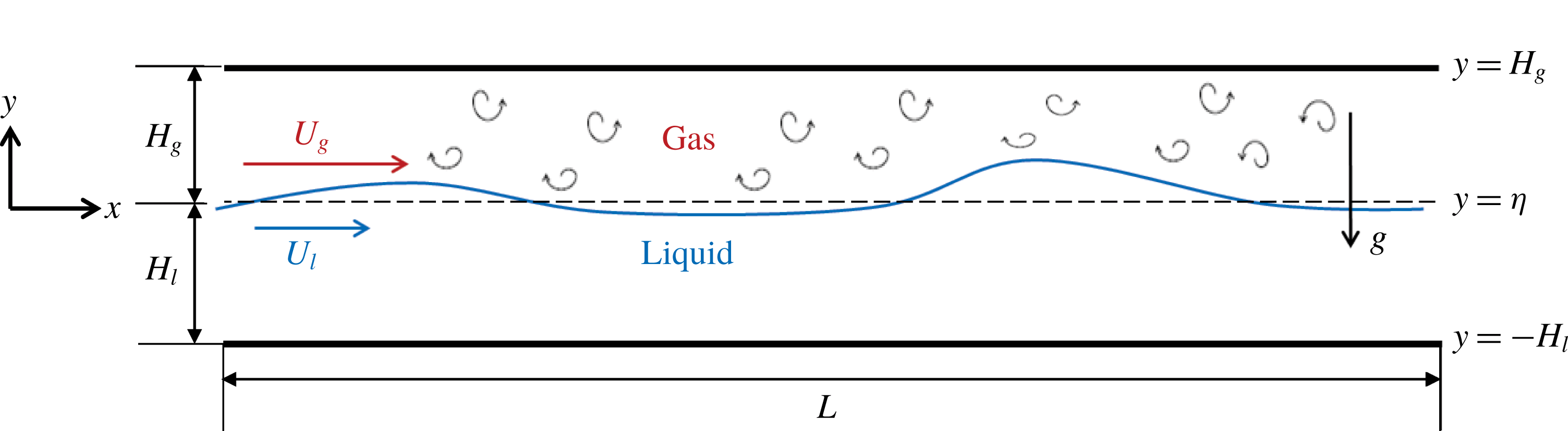
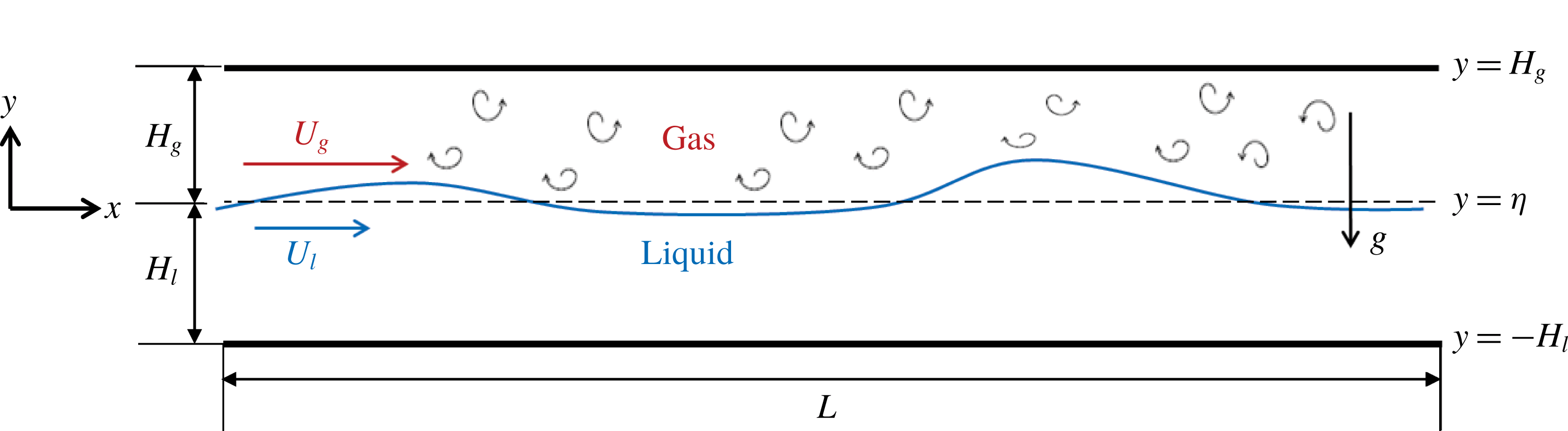
Sketch of a laminar liquid flow sheared by a co-current turbulent gas flow in a horizontal channel.
2 Problem statement and numerical method
2.1 Problem definition
We consider a co-current turbulent-gas/laminar-liquid flow driven by an external pressure drop
 $-\text{d}P/\text{d}x$
in a horizontal channel of length
 $L_{x}$
, as sketched in figure 1. The two fluids are immiscible, incompressible and Newtonian. The gas and liquid have respective densities
 $\unicode[STIX]{x1D70C}_{g}$
and
 $\unicode[STIX]{x1D70C}_{l}$
and dynamic viscosities
 $\unicode[STIX]{x1D707}_{g}$
and
 $\unicode[STIX]{x1D707}_{l}$
. The gas has an equilibrium depth
 $H_{g}$
with mean velocity
 $U_{g}$
, while the liquid has an equilibrium depth
 $H_{l}$
with mean velocity
 $U_{l}$
. We define the coordinate system with the origin located at the undisturbed interface at equilibrium with the
 $x$
(or
 $x_{1}$
) axis in the streamwise direction,
 $y$
(or
 $x_{2}$
) axis in the vertical direction and
 $z$
(or
 $x_{3}$
) axis in the spanwise direction. We describe the vertical displacement of the interface away from its undisturbed position by the function
 $y=\unicode[STIX]{x1D702}(x,z,t)$
, where
 $t$
denotes time. Scaling by
 $\unicode[STIX]{x1D70C}_{g}$
,
 $\unicode[STIX]{x1D707}_{g}$
,
 $H_{g}$
and a characteristic velocity
 ${\mathcal{U}}$
provides the following dimensionless governing parameters for this two-phase flow problem:
 $$\begin{eqnarray}\left.\begin{array}{@{}c@{}}\displaystyle Re=\frac{\unicode[STIX]{x1D70C}_{g}{\mathcal{U}}H_{g}}{\unicode[STIX]{x1D707}_{g}},\quad Fr=\frac{{\mathcal{U}}}{\sqrt{gH_{g}}},\quad P_{x}=\frac{-H_{g}{\displaystyle \frac{\text{d}P}{\text{d}x}}}{\unicode[STIX]{x1D70C}_{g}{\mathcal{U}}^{2}},\\ \displaystyle We=\frac{\unicode[STIX]{x1D6FE}}{\unicode[STIX]{x1D70C}_{g}{\mathcal{U}}^{2}H_{g}},\quad r=\frac{\unicode[STIX]{x1D70C}_{l}}{\unicode[STIX]{x1D70C}_{g}},\quad m=\frac{\unicode[STIX]{x1D707}_{l}}{\unicode[STIX]{x1D707}_{g}},\quad d=\frac{H_{l}}{H_{g}},\end{array}\right\}\end{eqnarray}$$
where
 $g$
is the gravitational acceleration and
 $\unicode[STIX]{x1D6FE}$
is the surface tension coefficient. We choose
 ${\mathcal{U}}$
such that we normalize the external pressure gradient
 $P_{x}$
to be 1. We also define two Reynolds numbers based on the mean velocity and equilibrium depth for each phase respectively:
 $$\begin{eqnarray}Re_{g}=\frac{\unicode[STIX]{x1D70C}_{g}U_{g}H_{g}}{\unicode[STIX]{x1D707}_{g}},\quad Re_{l}=\frac{\unicode[STIX]{x1D70C}_{l}U_{l}H_{l}}{\unicode[STIX]{x1D707}_{l}}.\end{eqnarray}$$
In this paper, we study the entire evolution from stratified flow to channel bridging for co-current turbulent-gas/laminar-liquid flows in horizontal channels. The goal is to identify the dominant mechanisms in distinctively different processes during the evolution leading to slugging. In particular, we focus our attention on two-phase flows with disparate Reynolds numbers:
 $Re_{g}\sim O(10^{3}){-}O(10^{5})$
and
 $Re_{l}\sim O(1){-}O(10^{2})$
.
2.2 Governing equations and numerical methods
We apply an FCIF solver (Miao et al. Reference Miao, Hendrickson and Liu2017) for the simulation of slug-generation processes in turbulent-gas/laminar-liquid horizontal channel flows. The FCIF solver captures dynamic interactions between two disparate fluids on a non-boundary-conforming grid by coupling two distinct flow solvers using an IB method or second-order boundary data immersion method (BDIM) (Maertens & Weymouth Reference Maertens and Weymouth2015).
Consider an immiscible two-phase problem where one fluid (e.g. gas) occupies domain
 $\unicode[STIX]{x1D6FA}_{g}$
with governing equation
 $G(\unicode[STIX]{x1D6F9})$
, and the other fluid (e.g. liquid) occupies domain
 $\unicode[STIX]{x1D6FA}_{l}$
with governing equation
 $L(\unicode[STIX]{x1D6F9})$
. Here
 $\unicode[STIX]{x1D6F9}$
represents the field quantities to be solved, such as velocities, turbulent kinetic energy (TKE), etc., and
 $S(\unicode[STIX]{x1D6F9})$
satisfies appropriate boundary conditions at the interface
 $\unicode[STIX]{x1D70E}_{s}$
. The general FCIF coupling framework solves a single smooth meta-equation
 $M_{\unicode[STIX]{x1D716}}(\unicode[STIX]{x1D6F9}_{\unicode[STIX]{x1D716}})$
throughout the whole domain
 $\unicode[STIX]{x1D6FA}$
comprising both phases by use of a nascent delta kernel
 $K_{\unicode[STIX]{x1D716}}$
of finite support
 $\unicode[STIX]{x1D716}$
over the interface
 $\unicode[STIX]{x1D70E}_{s}$
:
 $$\begin{eqnarray}\displaystyle M_{\unicode[STIX]{x1D716}}(\unicode[STIX]{x1D6F9}_{\unicode[STIX]{x1D716}}) & = & \displaystyle \int _{\unicode[STIX]{x1D6FA}_{g}}G(\unicode[STIX]{x1D6F9},\boldsymbol{x}_{g})K_{\unicode[STIX]{x1D716}}(\boldsymbol{x},\boldsymbol{x}_{g})\,\text{d}\boldsymbol{x}_{g}+\int _{\unicode[STIX]{x1D6FA}_{l}}L(\unicode[STIX]{x1D6F9},\boldsymbol{x}_{l})K_{\unicode[STIX]{x1D716}}(\boldsymbol{x},\boldsymbol{x}_{l})\,\text{d}\boldsymbol{x}_{l}\nonumber\\ \displaystyle & & \displaystyle +\,\int _{\unicode[STIX]{x1D70E}_{s}}S(\unicode[STIX]{x1D6F9},\boldsymbol{x}_{s})K_{\unicode[STIX]{x1D716}}(\boldsymbol{x},\boldsymbol{x}_{s})\,\text{d}\boldsymbol{x}_{s}\quad \text{for}~\boldsymbol{x}\in \unicode[STIX]{x1D6FA}.\end{eqnarray}$$
The formulation of the FCIF framework (2.3) guarantees a smooth transition from gas equations
 $G(\unicode[STIX]{x1D6F9})$
to liquid equations
 $L(\unicode[STIX]{x1D6F9})$
over the interface
 $\unicode[STIX]{x1D70E}_{s}$
within a small distance of
 $2\unicode[STIX]{x1D716}$
. It integrates the boundary information into the governing field equations and is grid independent, ensuring a straightforward implementation with minimal computational overhead.
For the slug-generation problem with turbulent gas over laminar liquid in a channel, we couple an unsteady Reynolds-averaged Navier–Stokes (uRANS) gas solver with a depth-integrated liquid solver (DIS) in the FCIF framework on a Cartesian grid. For the turbulent gas in the upper layer in figure 1, the governing incompressible uRANS equations
 $G(\unicode[STIX]{x1D6F9})$
are
 $$\begin{eqnarray}\displaystyle & \displaystyle \frac{\unicode[STIX]{x2202}u_{i}}{\unicode[STIX]{x2202}x_{i}}=0, & \displaystyle\end{eqnarray}$$
 $$\begin{eqnarray}\displaystyle & \displaystyle \frac{\unicode[STIX]{x2202}u_{i}}{\unicode[STIX]{x2202}t}+u_{j}\frac{\unicode[STIX]{x2202}u_{i}}{\unicode[STIX]{x2202}x_{j}}=-\frac{\unicode[STIX]{x2202}p}{\unicode[STIX]{x2202}x_{i}}+\frac{\unicode[STIX]{x2202}\unicode[STIX]{x1D70F}_{ij}}{\unicode[STIX]{x2202}x_{j}}, & \displaystyle\end{eqnarray}$$
where we normalize all the quantities by
 $H_{g}$
,
 $U_{g}$
and
 $\unicode[STIX]{x1D70C}_{g}$
in the gas layer. Here
 $u_{i}$
,
 $i=1,2,3$
, represents the Reynolds-averaged velocity components,
 $p$
is the Reynolds-averaged pressure, and
 $\unicode[STIX]{x1D70F}_{ij}$
is the total stress tensor, which is the sum of viscous stress and Reynolds stress. We model the turbulence with the Wilcox (Reference Wilcox1988)
 $k$
–
 $\unicode[STIX]{x1D714}$
turbulence closure model. We impose no-slip boundary conditions at both the top wall
 $y=H_{g}$
and the interface
 $y=\unicode[STIX]{x1D702}$
for the gas layer given the interfacial shape and velocities computed from the liquid solver because the interface acts like a wall to the gas motions owing to the large density ratio between liquid and gas (Angelis, Lombardi & Banerjee Reference Angelis, Lombardi and Banerjee1997; Liu et al.
Reference Liu, Kermani, Shen and Yue2009; Yang & Shen Reference Yang and Shen2011).
For the laminar liquid considered in the present study, the generated interfacial waves generally have wavelengths much longer than the liquid thickness as the high liquid viscosity damps out the short waves. This allows us to apply the standard long-wave model to describe the liquid motions (Benney Reference Benney1966; Shkadov Reference Shkadov1967; Lavalle et al.
Reference Lavalle, Vila, Blanchard, Laurent and Charru2015). We model the liquid as a laminar flow over a bottom wall subject to interfacial shear stress
 $\unicode[STIX]{x1D70F}_{\unicode[STIX]{x1D702}}^{i}$
,
 $i=1,3$
, and pressure
 $p_{\unicode[STIX]{x1D702}}$
computed from the uRANS gas solver. With the long-wave approximation, we derive the liquid governing equation
 $L(\unicode[STIX]{x1D6F9})$
by integrating the standard boundary layer equations over depth:
 $$\begin{eqnarray}\displaystyle & \displaystyle \frac{\unicode[STIX]{x2202}h}{\unicode[STIX]{x2202}t}+\frac{\unicode[STIX]{x2202}q_{i}}{\unicode[STIX]{x2202}x_{i}}=0, & \displaystyle\end{eqnarray}$$
 $$\begin{eqnarray}\displaystyle & \displaystyle \frac{\unicode[STIX]{x2202}q_{i}}{\unicode[STIX]{x2202}t}+\frac{\unicode[STIX]{x2202}I_{ij}}{\unicode[STIX]{x2202}x_{j}}=-\frac{h}{Fr_{l}^{2}}\frac{\unicode[STIX]{x2202}h}{\unicode[STIX]{x2202}x_{i}}+\frac{1}{Re_{l}}\left[\unicode[STIX]{x1D6E4}^{i}h+(\unicode[STIX]{x1D70F}_{\unicode[STIX]{x1D702}}^{i}-\unicode[STIX]{x1D70F}_{w}^{i})+\frac{\unicode[STIX]{x2202}}{\unicode[STIX]{x2202}x_{j}}\left(\frac{\unicode[STIX]{x2202}q_{i}}{\unicode[STIX]{x2202}x_{j}}+\frac{\unicode[STIX]{x2202}q_{j}}{\unicode[STIX]{x2202}x_{i}}\right)\right]+\frac{We_{l}h\unicode[STIX]{x2202}^{3}h}{\unicode[STIX]{x2202}x_{i}\unicode[STIX]{x2202}x_{j}\unicode[STIX]{x2202}x_{j}}, & \displaystyle \nonumber\\ \displaystyle & & \displaystyle\end{eqnarray}$$
where
 $h$
is the instantaneous liquid thickness,
 $q_{i}=\int _{-H_{l}}^{\unicode[STIX]{x1D702}}u_{i}\,\text{d}y$
is the flow rate,
 $\unicode[STIX]{x1D6E4}^{i}=Re_{l}\unicode[STIX]{x2202}p_{\unicode[STIX]{x1D702}}/\unicode[STIX]{x2202}x_{i}$
is the interfacial pressure gradient,
 $I_{ij}=6q_{i}q_{j}/(5h)+h^{3}(\unicode[STIX]{x1D70F}_{\unicode[STIX]{x1D702}}^{i}\unicode[STIX]{x1D6E4}^{j}h+\unicode[STIX]{x1D70F}_{\unicode[STIX]{x1D702}}^{j}\unicode[STIX]{x1D6E4}^{i}h+4\unicode[STIX]{x1D70F}_{\unicode[STIX]{x1D702}}^{i}\unicode[STIX]{x1D70F}_{\unicode[STIX]{x1D702}}^{j})/120$
is the integrated convection term and
 $\unicode[STIX]{x1D70F}_{w}^{i}=3q_{i}/h^{2}-\unicode[STIX]{x1D70F}_{\unicode[STIX]{x1D702}}^{i}/2$
is the bottom wall shear stress for
 $i,j=1,3$
. Here,
 $H_{l}$
,
 $U_{l}$
,
 $\unicode[STIX]{x1D70C}_{l}$
and
 $\unicode[STIX]{x1D707}_{l}$
are relevant scales with corresponding Froude and Weber numbers to be
 $Fr_{l}=U_{l}/\sqrt{gH_{l}}$
and
 $We_{l}=\unicode[STIX]{x1D6FE}/(\unicode[STIX]{x1D70C}_{l}U_{l}^{2}H_{l})$
.
As for the detailed coupling between uRANS and DIS, FCIF applies the following algorithm. At each time step of the simulation, uRANS provides the interfacial pressure gradient
 $\unicode[STIX]{x1D6E4}^{x,z}$
and shear stresses
 $\unicode[STIX]{x1D70F}_{\unicode[STIX]{x1D702}}^{x,z}$
to DIS as the driving force. The latter provides the interface geometry
 $\unicode[STIX]{x1D702}$
and velocity
 $u_{\unicode[STIX]{x1D702}}^{x,z}$
to uRANS as Dirichlet boundary conditions. Miao et al. (Reference Miao, Hendrickson and Liu2017) details the numerical implementation of FCIF including the application of second-order BDIM and the coupling scheme between the two solvers. We have performed extensive validations for FCIF to confirm its accuracy and efficacy in capturing the essential physics of gas–liquid interaction (see Miao et al.
Reference Miao, Hendrickson and Liu2017).
2.3 Simulation set-up
The experiments carried out by Andritsos et al. (Reference Andritsos, William and Hanratty1989) show the occurrence of wave coalescence phenomenon in the stratified–slug transition for a co-current turbulent-air/high-viscosity-liquid flow travelling through a horizontal pipe. Motivated by these experiments, we perform the numerical simulation (see figure 1) at similar flow conditions. We choose the physical parameters
 $Re=400.0$
,
 $Fr^{2}=2.5$
,
 $P_{x}=1.0$
,
 $r=1000.0$
,
 $m=5555.5$
and
 $d=2.0$
. The corresponding Reynolds numbers based on the mean flows for the two phases are
 $Re_{g}=4121.5$
and
 $Re_{l}=19.1$
, respectively. The surface tension effect is negligible for the two-phase problems we consider here, so we let
 $We=0$
. Recent simulations (e.g. Xie et al.
Reference Xie, Zheng, Triantafyllou, Constantinides, Zheng and Karniadakis2017) and our three-dimensional stability analysis in appendix A show that the dominant physics associated with the onset of slugging are two-dimensional, thus we choose a two-dimensional domain for our high-resolution simulation. The computational domain spans
 $(L_{x}/H_{g},L_{y}/H_{g})\in [0,20\unicode[STIX]{x03C0}]\times [-0.25,1]$
and the number of grid points is
 $(N_{x},N_{y})=(128,256)$
with
 $\unicode[STIX]{x0394}y^{+}=\simeq 1.66$
. We impose periodic boundary conditions in the streamwise direction and discretize the domain using uniform structured grids. Frank (Reference Frank2005) establishes that
 $L_{x}/D\sim 75$
is necessary for quantitative prediction of slug length/period when utilizing periodic boundary conditions, where
 $D$
is the pipe diameter. This work focuses on physical mechanisms associated with the onset of slugging rather than capturing the full slug length, thus our aspect ratio is less than this value. The freely evolving interface separating the two fluids is initially flat at
 $y=0$
. To capture the entire interfacial evolution under the effect of a turbulent gas flowing over a laminar liquid layer, we generate a stratified smooth base flow with a turbulent gas field as the initial condition. Once the base flow develops, we introduce white-noise perturbations at the flat interface to simulate the slug-generation processes.
To generate the base flow with a fully developed turbulence gas field over a laminar liquid layer, we initialize the simulation as a two-fluid laminar–laminar Poiseuille flow with a uniform TKE field (
 ${\sim}O(10^{-2})$
) in the gas domain. The interface remains flat throughout the development of the gas turbulence. The simulation evolves in time until the velocity field reaches a steady state. Figure 2(a,b) shows the resulting profile of the turbulent mean gas flow normalized respectively by interfacial velocity (
 $u_{\unicode[STIX]{x1D702}}^{\ast }$
) and wall-shear velocity (
 $u_{H}^{\ast }$
), where
 $u_{\unicode[STIX]{x1D702}/H}^{\ast }=\sqrt{\unicode[STIX]{x1D70F}_{\unicode[STIX]{x1D702}/H}}$
. The present simulation result agrees well with the linear law of the wall profile in the viscous sub-layers and the log-law profiles in the logarithmic regions. It also compares well with the approximation from Náraigh et al. (Reference Náraigh, Spelt, Matar and Zaki2011a
).
Mean velocity profile for (a) interfacial region and (b) wall region: ○ (blue), present numerical simulation by FCIF solver; —— (red), approximation from Náraigh et al. (Reference Náraigh, Spelt, Matar and Zaki2011a
); – – –, theoretical asymptotics for viscous sub-layer and log layers. The linear laws for the viscous sub-layers of the interfacial and wall regions are
 $u_{\unicode[STIX]{x1D702}}^{+}=u(0){\mathcal{U}}/u_{\unicode[STIX]{x1D702}}^{\ast }+y_{i}^{+}$
and
 $u_{H}^{+}=y_{H}^{+}$
, respectively. The log-law for the logarithmic regions is
 $u_{\unicode[STIX]{x1D702}/H}^{+}=(1/\unicode[STIX]{x1D705})\log y^{+}+B_{\unicode[STIX]{x1D702}/H}$
with
 $\unicode[STIX]{x1D705}=0.41$
,
 $B_{\unicode[STIX]{x1D702}}=6$
and
 $B_{H}=5.1$
.

With the initial base flow established, we then consider the slug generation by introducing small-amplitude white noise at the flat interface. We continue the simulation until the interface (nearly) bridges the channel leading to slugging.
3 Characteristics of interface evolution towards slugging
Space–time waterfall plot of the interface evolution at
 $Re_{l}=19.1$
and
 $Re_{g}=4121.5$
. The domain is tripled in the streamwise direction for visual purposes. The shading of the plot represents the liquid depth, following the colour bar on the right.

Successive profiles of the gas–liquid interface during time evolution of the slug development. Note that the vertical scale for the vertical elevation of the interface differs in each panel of figures for better visualization of the characteristics of interfacial profile evolution (
 $Re_{l}=19.1$
and
 $Re_{g}=4121.5$
). The wave peak scale stands for around 0.02 (a), 0.5 (b) and 1.0 (c), respectively, which are non-dimensionalized with respect to the gas equilibrium height
 $H_{g}$
(equal to
 $1/3$
of the channel height).

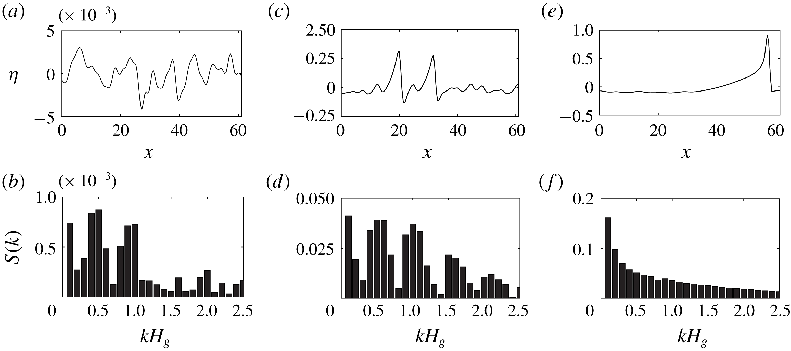
Wave elevation
 $\unicode[STIX]{x1D702}$
and the corresponding Fourier spectrum
 $S(k)$
at
 $t=8$
(a,b),
 $t=130$
(c,d) and
 $t=210$
(e,f).

Figure 3 displays the spatio-temporal evolution of the gas–liquid interface under the influence of turbulent gas flow. The lines in this space–time plot show the trace of peaks of the travelling waves, with their inverse slope corresponding to the wave speed. Brighter regions correspond to small wave amplitudes, whereas darker regions correspond to large wave amplitudes. The bending and shading of several distinct dark lines at
 $t>120$
implies that larger waves travel faster. These larger waves accelerate and gain mass by absorbing slower waves (indicated by the darkening of the line) through rapid sequences of wave coalescence.
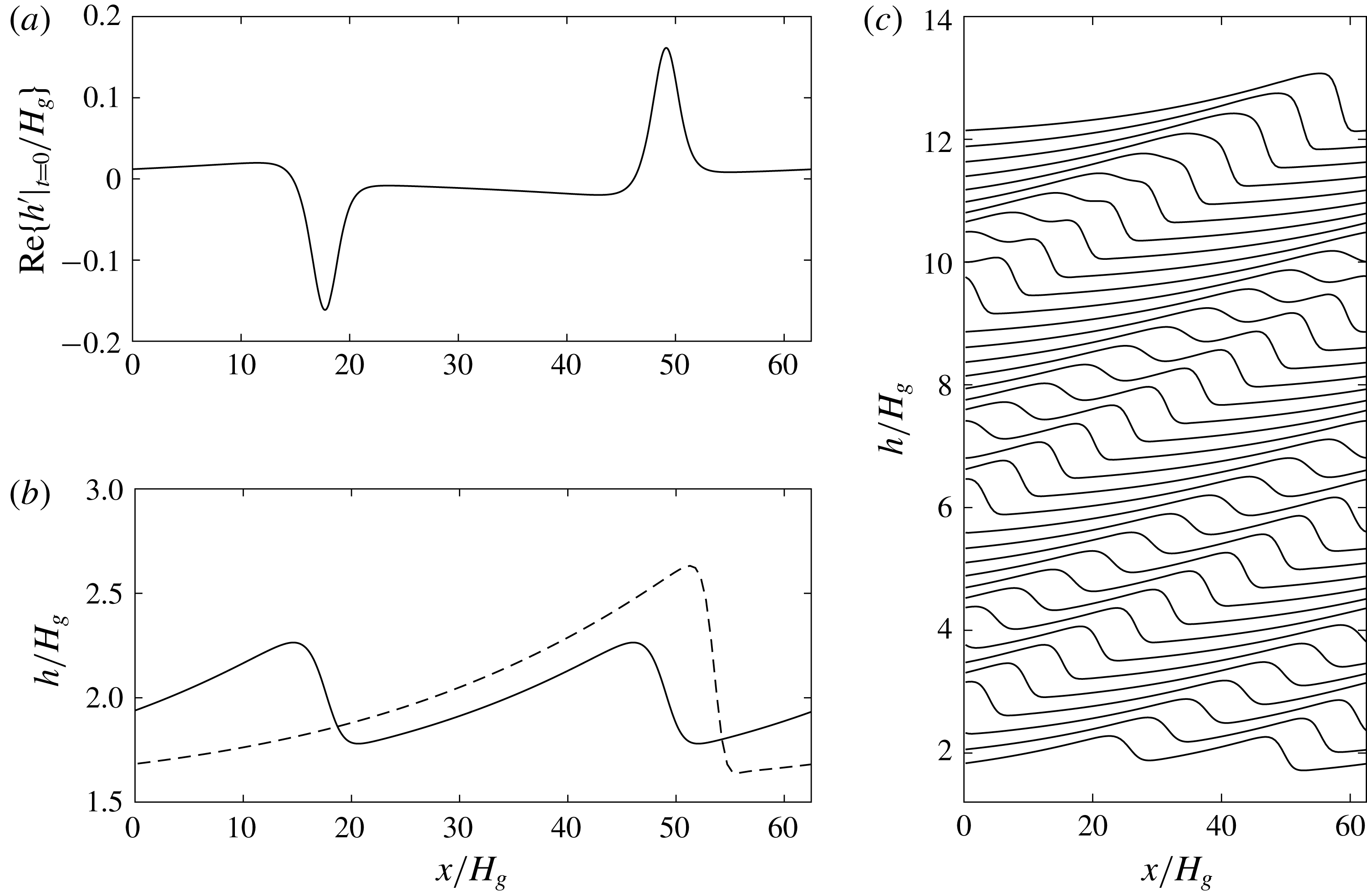
Figure 4 shows the successive profile evolution during the slug generation. We establish the slug formation through three major processes. In Process I (
 $t=0{-}O(50)$
in figure 4
a), the initial perturbations produce short ripples that grow larger and longer as the nonlinear effect becomes relevant. In Process II (
 $t=O(50){-}O(200)$
in figure 4
b,c), short waves saturate and long solitary waves form at the interface due to a series of wave coalescences. These long irregular waves have steep wave fronts and smooth tails, which resemble experimental observations (Andritsos & Hanratty Reference Andritsos and Hanratty1987b
; Andritsos et al.
Reference Andritsos, William and Hanratty1989; Jurman & McCready Reference Jurman and McCready1989). The characteristic features of wave coalescence leading to the initiation of slug flow for the high-density gas flow over high-viscous liquid also agree qualitatively with those found in the two-phase air/water simulation of Höhne & Mehlhoop (Reference Höhne and Mehlhoop2014). In Process III, one solitary wave grows by sweeping up enough intermediate waves such that its crest approaches the top wall rapidly with a time scale
 ${\sim}O(10^{-1})$
, leading to slugging with a nearly flat interface in its wake (see the top of figures 4
c and 5
e).
Figure 5 shows analysis of the Fourier spectra of the wave elevation throughout these three processes. We observe a clear shift in energy from shorter to longer waves as slug develops. In the following sections, we detail these three processes of the slug formation and study the dominant physics in each process.
4 Process I: linear interfacial instabilities
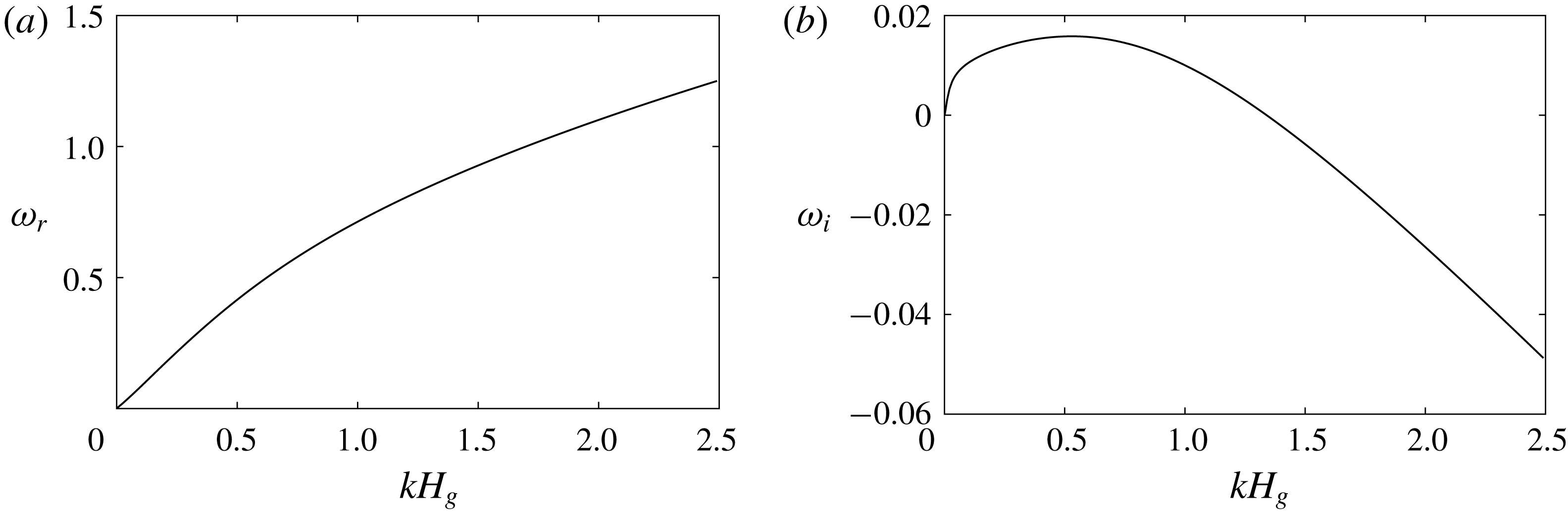
(a) Linear wave frequency and (b) growth-rate spectrum computed using the quasi-laminar hypothesis and the approximated mean velocity profile based on the model in Náraigh et al. (Reference Náraigh, Spelt, Matar and Zaki2011a
) for
 $Re_{l}=19.1$
and
 $Re_{g}=4121.5$
.

Process I is the growth of minuscule waves through linear interfacial instabilities. It begins with a flat interface and continues until nonlinearity dominates the wave growth (near
 $t=35$
in figure 4
a). Performing the linear instability analysis for the full system of the governing equations for this turbulent-gas/laminar-liquid flow is a formidable task. Thus, we follow a simplified analysis approach by Náraigh et al. (Reference Náraigh, Spelt, Matar and Zaki2011a
), which utilizes the approximated base flow velocity profile (denoted as the red solid lines in figure 2) and the quasi-laminar (QL) hypothesis that neglects wave-induced Reynolds stress. We solve the resulting linearized TOS equations for the linear wave frequency and growth-rate spectrum of the stratified base flow. Figure 6(a) shows that the linear wave frequency
 $\unicode[STIX]{x1D714}_{r}$
experiences a nearly linear dependence on wavenumbers
 $k$
for
 $kH_{g}<0.5$
. The growth-rate spectrum, shown in figure 6(b), presents an unstable band of wavenumbers in the long-wave regime from
 $kH_{g}=0$
to
 $kH_{g}\simeq 1.3$
, with the peak growth rate occurring at
 $kH_{g}\simeq 0.5$
. Table 1 presents a quantitative comparison of the dispersion relation between this theoretical approximation and our numerical estimates from the FCIF simulation for the first few harmonic wave modes in the present computational domain. Overall we obtain good agreement for these long-wave modes, which is consistent with the long-wave assumption employed in the FCIF solver. The difference in the turbulence model for Reynolds stress (
 $k{-}\unicode[STIX]{x1D714}$
model in our FCIF numerical simulation; QL hypothesis in TOS theoretical prediction) and the nonlinear adjustments to the dispersion relationship are potential reasons for the discrepancies between the theoretical and numerical estimates of the wave frequencies. This validation confirms that the linear interfacial instability governs the initial transition from stratified to wavy flows in Process I (Valluri et al.
Reference Valluri, Spelt, Lawrence and Hewitt2008, Reference Valluri, Náraigh, Ding and Spelt2010; Campbell et al.
Reference Campbell, Hendrickson and Liu2016). Quantitative comparison of the initial wave growth rate from our FCIF simulation (with
 $k{-}\unicode[STIX]{x1D714}$
model and long-wave assumption) and the theoretical TOS prediction (with QL model) is not possible because: (1) the DIS used in the FCIF simulation is only accurate to leading order (
 $O(1)$
) and the wave growth rate
 $\unicode[STIX]{x1D714}_{i}$
is a first-order (
 $O(kH_{l})$
) quantity in the long-wave limit
 $kH_{l}\ll 1$
; and (2) the QL model used in the TOS prediction is known to introduce large errors in the wall shear stress phase angle at long-wave regime (for example, in turbulent flows over solid wavy surfaces in the long-wave regime in figure 5 of Abrams & Hanratty Reference Abrams and Hanratty1985).
Comparison of interfacial modal frequencies between numerical evaluations from the FCIF solver (
 $\unicode[STIX]{x1D714}_{r}^{N}$
) and theoretical approximations following the analysis in Náraigh et al. (Reference Náraigh, Spelt, Matar and Zaki2011a
) (
 $\unicode[STIX]{x1D714}_{r}^{T}$
). Here
 $k_{j}$
denotes the interfacial wavenumber.

5 Process II: nonlinear wave coalescence
The monochromatic waves induced by linear interfacial instabilities in Process I gradually evolve into travelling solitary humps with steep fronts and smooth tails through nonlinear resonant and near-resonant wave–wave interactions in Process II (see figure 4 b). These solitary humps travel faster than the monochromatic waves without much variation in shape and resemble the periodic solitary-wave solutions for free-falling thin films (Chang et al. Reference Chang, Demekhin and Kopelevich1993) or the roll waves for the inclined open channels of shallow-water flows (Needham & Merkin Reference Needham and Merkin1984). As these humps propagate downstream, they further coalesce to form an even longer and larger-amplitude hump which will bridge the channel to form slugging (see figure 4 c).
5.1 Formation of periodic solitary waves
To assist in understanding this complex process observed in FCIF simulation, we first consider a simpler one-way interaction problem with a laminar liquid layer driven by constant interfacial forces based on numerical analysis on the liquid governing equations (2.6) and (2.7). We only consider the nonlinearity of interfacial waves sheared by a turbulent gas flow without invoking the influence of these waves on the turbulent gas. Under this assumption, we can approximate the gas flow as a steady Poiseuille flow producing the following constant interfacial forces:
 $$\begin{eqnarray}-\frac{\text{d}p_{\unicode[STIX]{x1D702}}}{\text{d}x}=\frac{2\unicode[STIX]{x1D70F}_{\unicode[STIX]{x1D702}}^{x}}{H_{g}},\quad \frac{\text{d}p_{\unicode[STIX]{x1D702}}}{\text{d}z}=\unicode[STIX]{x1D70F}_{\unicode[STIX]{x1D702}}^{z}=0.\end{eqnarray}$$
From the interfacial forcing terms in (2.6) and (2.7), we obtain that the liquid hold-up
 $$\begin{eqnarray}R_{f}=2d=\frac{-{\displaystyle \frac{\text{d}p_{\unicode[STIX]{x1D702}}}{\text{d}x}}H_{l}}{\unicode[STIX]{x1D70F}_{\unicode[STIX]{x1D702}}^{x}}\end{eqnarray}$$
characterizes the strength ratio between the pressure and shear stress forcing from the gas, where the definition of depth ratio
 $d$
is consistent with that in simulation defined in (2.1).
We rewrite (2.6) and (2.7) in a frame of reference moving with speed
 $c$
in the streamwise direction:
 $$\begin{eqnarray}\frac{\unicode[STIX]{x2202}h}{\unicode[STIX]{x2202}t}+\frac{\unicode[STIX]{x2202}q_{x}}{\unicode[STIX]{x2202}x}+\frac{\unicode[STIX]{x2202}q_{z}}{\unicode[STIX]{x2202}z}=c\frac{\unicode[STIX]{x2202}h}{\unicode[STIX]{x2202}x},\end{eqnarray}$$
 $$\begin{eqnarray}\displaystyle \frac{\unicode[STIX]{x2202}q_{x}}{\unicode[STIX]{x2202}t}+\frac{\unicode[STIX]{x2202}I_{xx}}{\unicode[STIX]{x2202}x}+\frac{\unicode[STIX]{x2202}I_{xz}}{\unicode[STIX]{x2202}z} & = & \displaystyle c\frac{\unicode[STIX]{x2202}q_{x}}{\unicode[STIX]{x2202}x}-\frac{h}{Fr_{l}^{2}}\frac{\unicode[STIX]{x2202}h}{\unicode[STIX]{x2202}x}+\frac{\unicode[STIX]{x1D6E4}^{x}}{Re_{l}}h+\frac{1}{Re_{l}}\nonumber\\ \displaystyle & & \displaystyle \times \left[(\unicode[STIX]{x1D70F}_{\unicode[STIX]{x1D702}}^{x}-\unicode[STIX]{x1D70F}_{w}^{x})+\frac{\unicode[STIX]{x2202}}{\unicode[STIX]{x2202}x}\left(2\frac{\unicode[STIX]{x2202}q_{x}}{\unicode[STIX]{x2202}x}\right)+\frac{\unicode[STIX]{x2202}}{\unicode[STIX]{x2202}z}\left(\frac{\unicode[STIX]{x2202}q_{x}}{\unicode[STIX]{x2202}z}+\frac{\unicode[STIX]{x2202}q_{z}}{\unicode[STIX]{x2202}x}\right)\right]\nonumber\\ \displaystyle & & \displaystyle +\,We_{l}h\left(\frac{\unicode[STIX]{x2202}^{3}h}{\unicode[STIX]{x2202}x^{3}}+\frac{\unicode[STIX]{x2202}^{3}h}{\unicode[STIX]{x2202}x\unicode[STIX]{x2202}z^{2}}\right),\end{eqnarray}$$
 $$\begin{eqnarray}\displaystyle \frac{\unicode[STIX]{x2202}q_{z}}{\unicode[STIX]{x2202}t}+\frac{\unicode[STIX]{x2202}I_{xz}}{\unicode[STIX]{x2202}x}+\frac{\unicode[STIX]{x2202}I_{zz}}{\unicode[STIX]{x2202}z} & = & \displaystyle c\frac{\unicode[STIX]{x2202}q_{z}}{\unicode[STIX]{x2202}x}-\frac{h}{Fr_{l}^{2}}\frac{\unicode[STIX]{x2202}h}{\unicode[STIX]{x2202}z}+\frac{\unicode[STIX]{x1D6E4}^{z}}{Re_{l}}h+\frac{1}{Re_{l}}\nonumber\\ \displaystyle & & \displaystyle \times \left[(\unicode[STIX]{x1D70F}_{\unicode[STIX]{x1D702}}^{z}-\unicode[STIX]{x1D70F}_{w}^{z})+\frac{\unicode[STIX]{x2202}}{\unicode[STIX]{x2202}x}\left(\frac{\unicode[STIX]{x2202}q_{x}}{\unicode[STIX]{x2202}z}+\frac{\unicode[STIX]{x2202}q_{z}}{\unicode[STIX]{x2202}x}\right)+\frac{\unicode[STIX]{x2202}}{\unicode[STIX]{x2202}z}\left(2\frac{\unicode[STIX]{x2202}q_{z}}{\unicode[STIX]{x2202}z}\right)\right]\nonumber\\ \displaystyle & & \displaystyle +\,We_{l}h\left(\frac{\unicode[STIX]{x2202}^{3}h}{\unicode[STIX]{x2202}x^{2}\unicode[STIX]{x2202}z}+\frac{\unicode[STIX]{x2202}^{3}h}{\unicode[STIX]{x2202}z^{3}}\right).\end{eqnarray}$$
We have retained the same independent variable ‘
 $x$
’ for the moving coordinate for convenience. We seek two-dimensional periodic steady-state solutions (
 $\unicode[STIX]{x2202}/\unicode[STIX]{x2202}t=\unicode[STIX]{x2202}/\unicode[STIX]{x2202}z=0$
,
 $q_{z}=0$
) of (5.3)–(5.5) with constant interfacial forcing (5.1). Integrating (5.3) once, we obtain
 $$\begin{eqnarray}q_{x}=ch+C_{0},\end{eqnarray}$$
where
 $C_{0}$
is the constant of integration depending on the initial liquid flow rate. Since we introduce additional unknowns
 $C_{0}$
and
 $c$
, we impose a derivative condition
 $\unicode[STIX]{x2202}h/\unicode[STIX]{x2202}x|_{x=0}=0$
and an integral condition for constant mass under one wave
 $\int _{-\unicode[STIX]{x03C0}/k_{0}}^{\unicode[STIX]{x03C0}/k_{0}}h\,\text{d}x=2\unicode[STIX]{x03C0}/k_{0}$
, where
 $k_{0}$
is the wavenumber of periodic solution. Eliminating
 $q_{x}$
by (5.6), we numerically solve (5.4) together with the derivative and integral conditions to obtain the nonlinear steady wave solution for given
 $k_{0}$
. For this one-way interaction problem, we consider similar flow conditions as in the two-way interaction simulation by FCIF:
 $Re_{l}=19.1$
,
 $Fr_{l}=1.32$
,
 $We_{l}=0.0$
,
 $r=1000.0$
and
 $m=5555.5$
. We consider different depth ratios
 $d=1/2,1,2$
to study the characteristics of the nonlinear periodic waves driven by interfacial forces with different pressure-to-shear ratios
 $R_{f}$
.
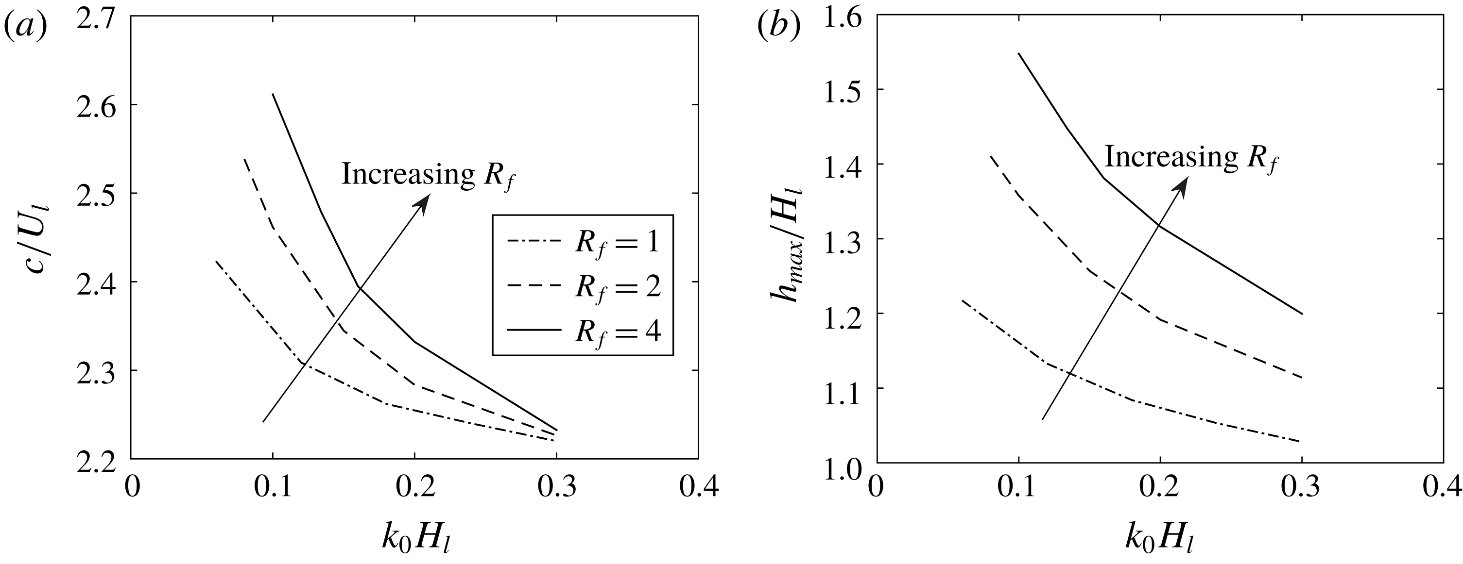
Figure 7 shows the dependence of the travelling speed
 $c$
and maximum wave elevation
 $h_{max}$
of the nonlinear periodic waves on different
 $k_{0}$
with various
 $R_{f}(d)$
for this one-way interaction problem. For a given
 $R_{f}(d)$
, there exists a one-parameter family of nonlinear periodic travelling-wave solutions parametrized by their wavenumber
 $k_{0}$
, similar to the one-layer free-falling thin films or the inclined shallow-water flows (Needham & Merkin Reference Needham and Merkin1984; Hwang & Chang Reference Hwang and Chang1987; Prokopiou, Cheng & Chang Reference Prokopiou, Cheng and Chang1991). These periodic waves correspond to limit cycles branched out from the Hopf bifurcation point of the flat-interface base state in the phase plane. In addition, longer waves have larger amplitudes and travel faster for a given
 $R_{f}(d)$
. For a given
 $k_{0}$
, increasing the interfacial pressure-to-shear strength ratio
 $R_{f}$
results in larger wave amplitude and travelling speed. This implies that interfacial pressure gradient transfers energy to liquid more efficiently than the shear stress.
(a) Travelling speed
 $c$
and (b) maximum wave height
 $h_{max}$
of the periodic solitary waves as functions of
 $k_{0}H_{l}$
with different interfacial pressure-to-shear strength ratios
 $R_{f}$
(i.e. different liquid hold-ups
 $d$
) for the one-way interaction problem.

(a) Wave elevation profile, (b) relative depth-averaged streamwise velocity magnitude
 $|q_{x}/h-c|$
and (c) corresponding Fourier spectrum of a steady periodic solitary wave of
 $k_{0}H_{l}=0.06$
in the one-way interaction problem for
 $d=1/2$
in the frame of reference moving with the wave speed
 $c/U_{l}=2.53$
. In this moving frame, the relative liquid velocity is from right to left.

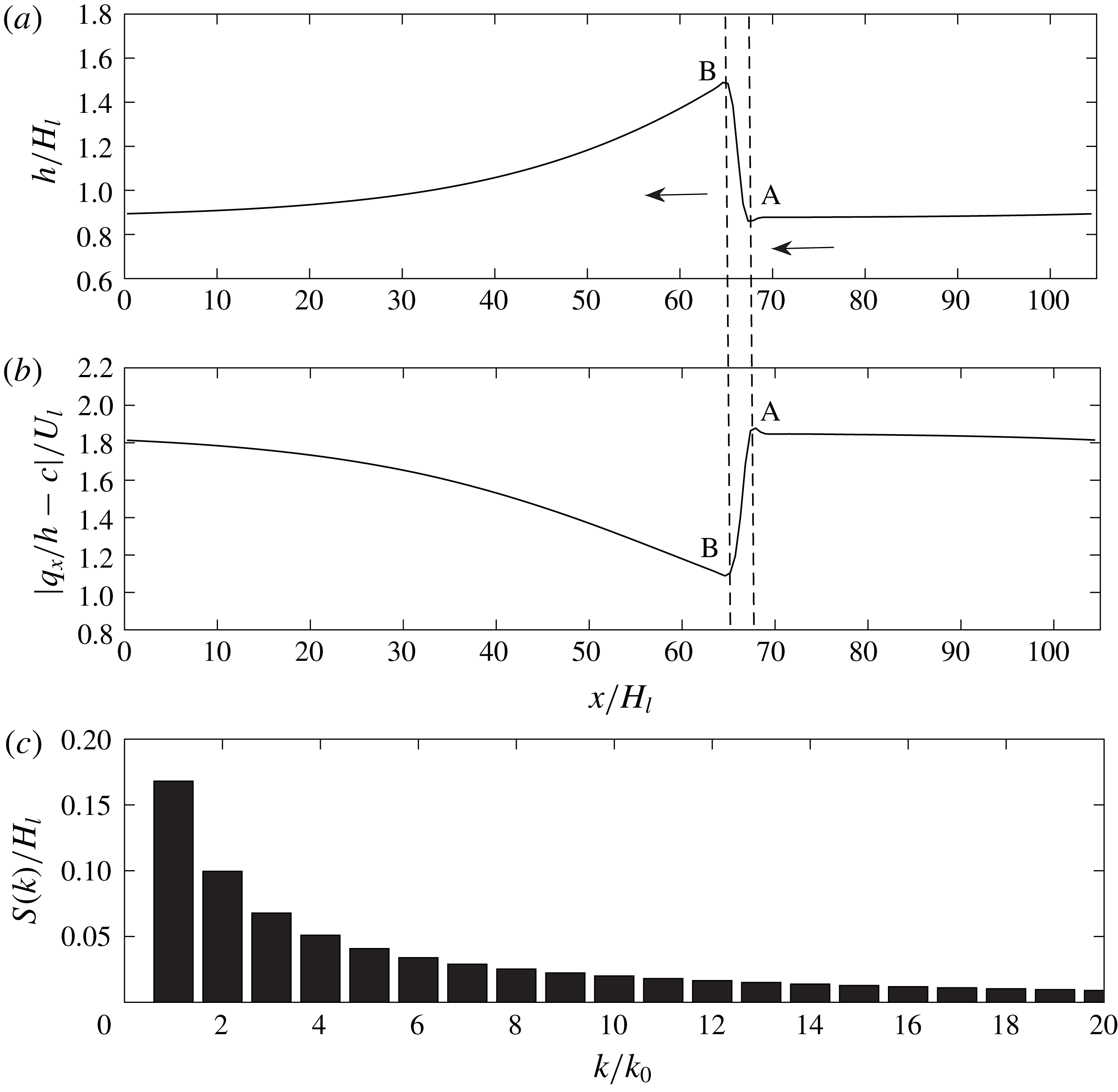
All of these nonlinear waves present a soliton-like shape but asymmetric with the wave front steeper than the back tail, similar to the solitary waves we observe in the two-way interaction simulation by FCIF (see figure 4). Figure 8 shows a typical periodic solitary wave of
 $k_{0}H_{l}=0.06$
with
 $d=1/2$
in a frame travelling with its wave speed
 $c/U_{l}=2.53$
. In this moving frame, the liquid flows from right to left with a constant relative flow rate
 $q_{rel}=q_{x}-ch=C_{0}$
. The relative flow velocity drops significantly from
 $A$
to
 $B$
with an abrupt rise of the interface, similar to a stationary hydraulic jump. The corresponding Fourier spectrum of this single solitary wave of
 $k_{0}$
comprises many Fourier modes
 $k_{0}$
,
 $2k_{0}$
,
 $3k_{0},\ldots .$
These flow characteristics are consistent with experimental observations (Jurman, Bruno & McCready Reference Jurman, Bruno and McCready1989; Jurman & McCready Reference Jurman and McCready1989; Jepson Reference Jepson1990).
(a) Modal amplitude evolution of the first five Fourier modes during the evolution from flat interface with small white noise to the steady solitary wave of
 $k_{0}H_{l}=0.06$
under constant interfacial forces with
 $d=1/2$
; (b) the corresponding trajectory (– – –) from the Hopf point
 $(1,0)$
(equilibrium for a flat interface) to the solitary wave in the phase-plane diagram. Here —— (red) denotes the limit cycle corresponding to the periodic solitary wave.

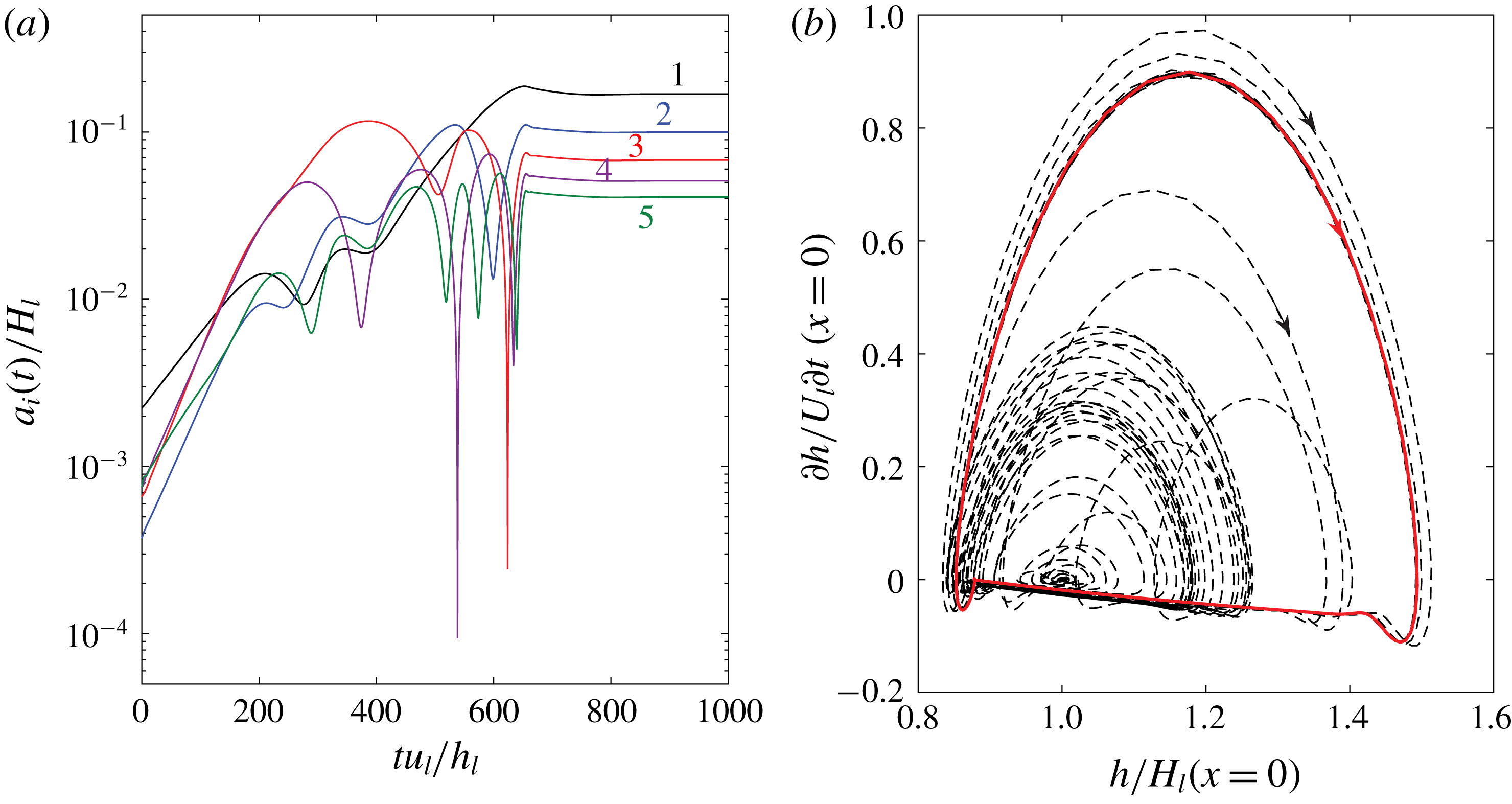
The evolution from the flat interface to any of these periodic solitary waves involves linear interfacial instabilities and nonlinear wave–wave interactions that may directly lead to slugging for relatively low superficial gas velocities (Campbell & Liu Reference Campbell and Liu2013; Campbell et al.
Reference Campbell, Hendrickson and Liu2016). As an illustration, figure 9 provides a sample evolution process of generating the solitary wave in figure 8 starting from a flat interface with small-amplitude white-noise perturbations. A linear interfacial stability analysis of (2.6) and (2.7) for the flat-interface base flow of this one-way interaction problem obtains a weakly dispersive and linearly unstable Fourier spectrum in the long-wave regime, similar to Process I of the two-way interaction problem (figure 6). As these weakly dispersive Fourier waves grow from the effect of linear instability, they generate new free Fourier waves and transfer energy among them through (triad and higher-order) resonant and/or near-resonant wave–wave interactions (Phillips Reference Phillips1960; Chang Reference Chang1994; Campbell et al.
Reference Campbell, Hendrickson and Liu2016). Figure 9(a) confirms that the amplitudes of the fundamental Fourier mode and its first few harmonics grow exponentially initially following the linear instability, then oscillate in time exchanging energy among them due to nonlinear near-resonant wave–wave interactions, and eventually saturate at the equilibrium values when the steady solitary wave forms. We also plot the corresponding trajectory in the phase plane of
 $(h,\text{d}h/\text{d}t)$
at
 $x=0$
, as shown in figure 9(b). The trajectory path spirals out from the Hopf point
 $(1,0)$
, eventually settling down at a limit cycle corresponding to the steady periodic solitary wave solution.
To construct a quantitative measure of nonlinear triad resonant wave interactions when a solitary wave forms, we define the following bi-coherence:
 $$\begin{eqnarray}Bi(k_{1},k_{2})=\frac{|\langle a_{1}^{\ast }(k_{1})a_{2}(k_{2})a_{3}(k_{3}=k_{1}+k_{2})\rangle |}{\langle |a_{1}(k_{1})||a_{2}(k_{2})||a_{3}(k_{3}=k_{1}+k_{2})|\rangle },\end{eqnarray}$$
with
 $\langle \,\rangle$
denoting the time average,
 $\ast$
the complex conjugate and
 $a_{i}(k_{i})$
the spatial Fourier component of the wave elevation at wavenumber
 $k_{i}$
. Here
 $Bi$
measures the phase coupling of the three Fourier wave components
 $k_{1}$
,
 $k_{2}$
and
 $k_{3}=k_{1}+k_{2}$
. The bi-coherence
 $Bi$
has the value in the range of 0 to 1 with
 $Bi=0$
(or 1) corresponding to completely no (or perfect) coupling among the three wave modes. In general,
 $Bi$
obtains high values for resonant and near-resonant triads of
 $(k_{1},k_{2},k_{3})$
which satisfy the condition
 $\text{Re}\{\unicode[STIX]{x1D714}_{3}-\unicode[STIX]{x1D714}_{1}-\unicode[STIX]{x1D714}_{2}\}=\unicode[STIX]{x1D6FF}$
,
 $\unicode[STIX]{x1D6FF}\ll 1$
, and low values for non-resonant triads. We compute
 $Bi(k_{1},k_{2})$
when the steady solitary wave in figure 9 forms. We obtain
 $Bi(k_{1},k_{2})>0.9998$
for any
 $k_{1}/k_{0},k_{2}/k_{0}=1,2,\ldots ,15$
. This means that the weak dispersion of the Fourier waves leads to near-resonance triads for any three of them. Eventually through multiple resonant and near-resonant interactions, all the Fourier modes
 $k_{0},2k_{0},3k_{0},\ldots$
are phase-locked into one solitary hump of
 $k_{0}$
. This nonlinear process is different from the one or two dominant (near-)resonance triads that lead to slugging for relatively low gas flow rates (Campbell & Liu Reference Campbell and Liu2013; Campbell et al.
Reference Campbell, Hendrickson and Liu2016). Examination of the bi-coherence of the solitary wave developed at the end of Process II in the two-way interaction simulation (figure 4
c) obtains the same features.
5.2 Coalescence of solitary waves
We note from figure 4(c) that two long solitary waves further coalesce to form a longer one at
 $t\sim O(200)$
in the FCIF simulation. We attribute the mechanism behind this solitary wave coalescence to their subharmonic instabilities. To illustrate this mechanism, we study the instability of a two-dimensional periodic solitary wave of wavenumber
 $k_{0}$
, which we derive for the one-way interaction problem in § 5.1, subject to an infinitesimal three-dimensional disturbance. Appendix A details the stability analysis.
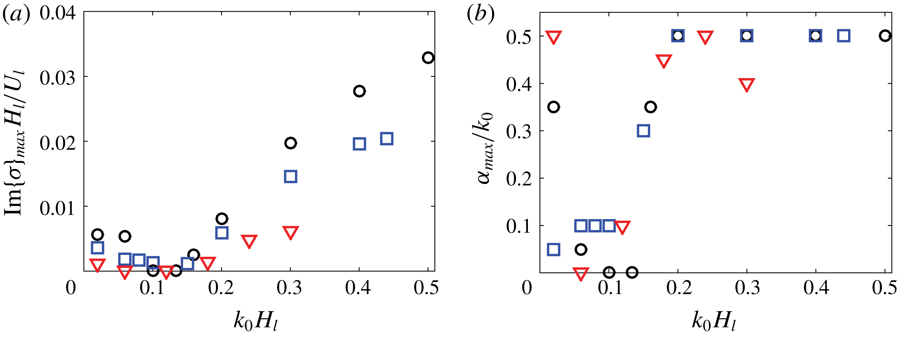
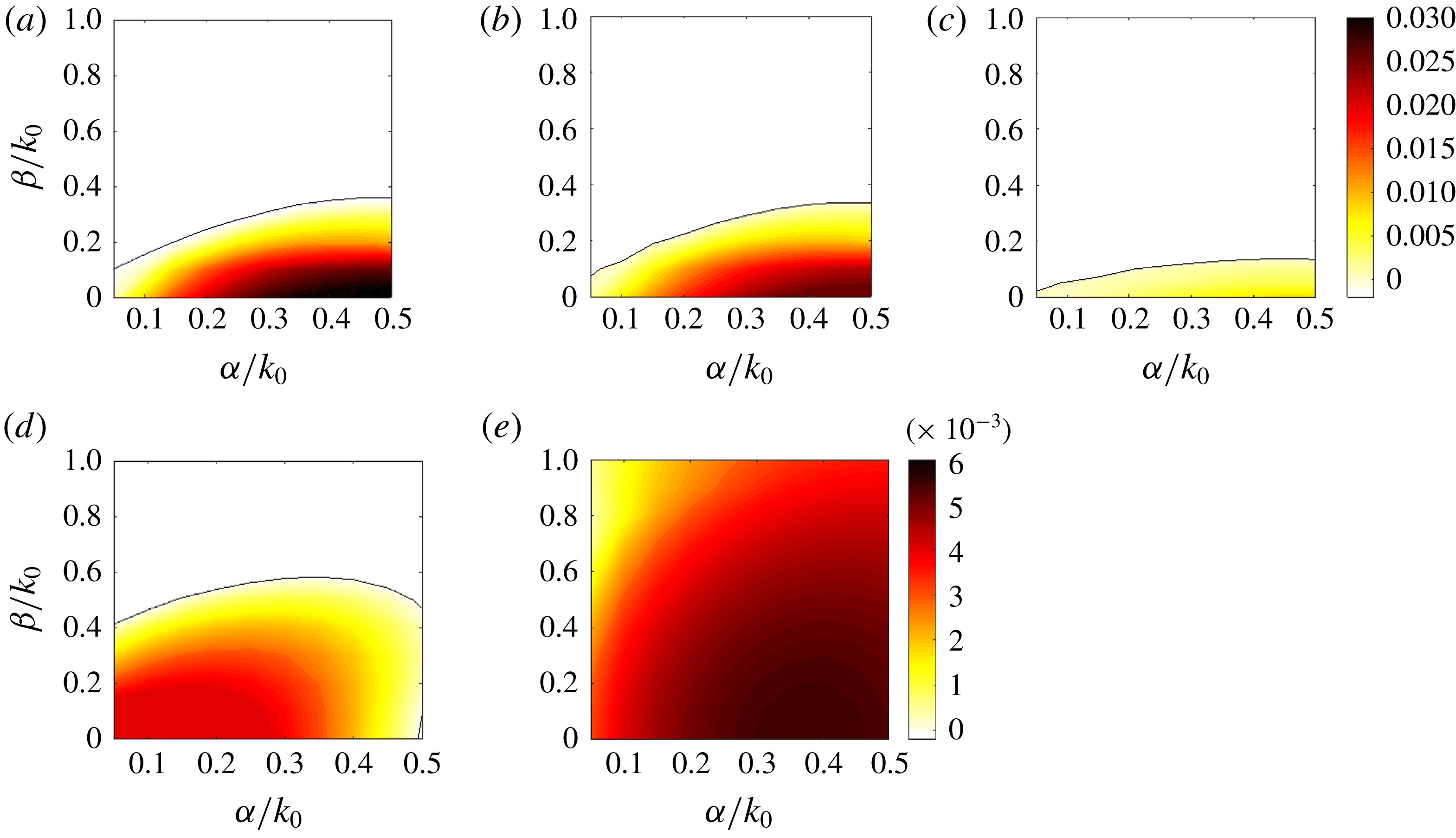
We focus here on the two-dimensional instability of the periodic solitary waves. Appendix A provides several typical three-dimensional instability results for solitary waves of different steepness, which justifies that the instability is dominantly two-dimensional. We study the dependence of the maximum two-dimensional perturbation growth rates on the steepness of solitary waves and the interfacial pressure-to-shear strength ratio
 $R_{f}$
, as shown in figure 10. Under constant interfacial forcings, we find that periodic solitary waves in a wide range of steepness, particularly for short steep waves, are unstable to subharmonic disturbances (
 $\unicode[STIX]{x1D6FC}/k_{0}<1$
), where
 $\unicode[STIX]{x1D6FC}$
is the wavenumber of the disturbances in the streamwise direction. This destabilization mechanism would create a cascade of solitary wave coarsening until the resulting waves either touch the channel/pipe top or become stable. Figure 10 also reveals that a larger pressure-to-shear strength ratio tends to produce a stronger subharmonic instability.
To further illustrate that this destabilization mechanism is responsible for the wave coalescence in the FCIF simulation, we approximate the two large irregular waves at
 $t\sim O(160)$
(figure 4
c) by a periodic solitary wave train in the one-way interaction problem with the same depth ratio
 $d=2$
. We choose the solitary wavenumber
 $k_{0}$
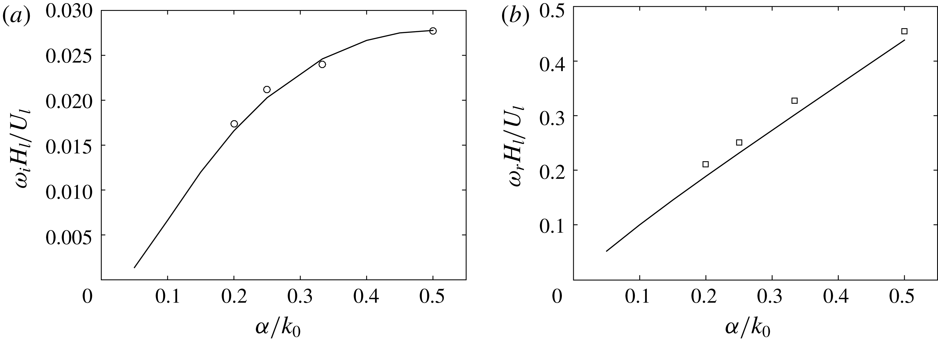
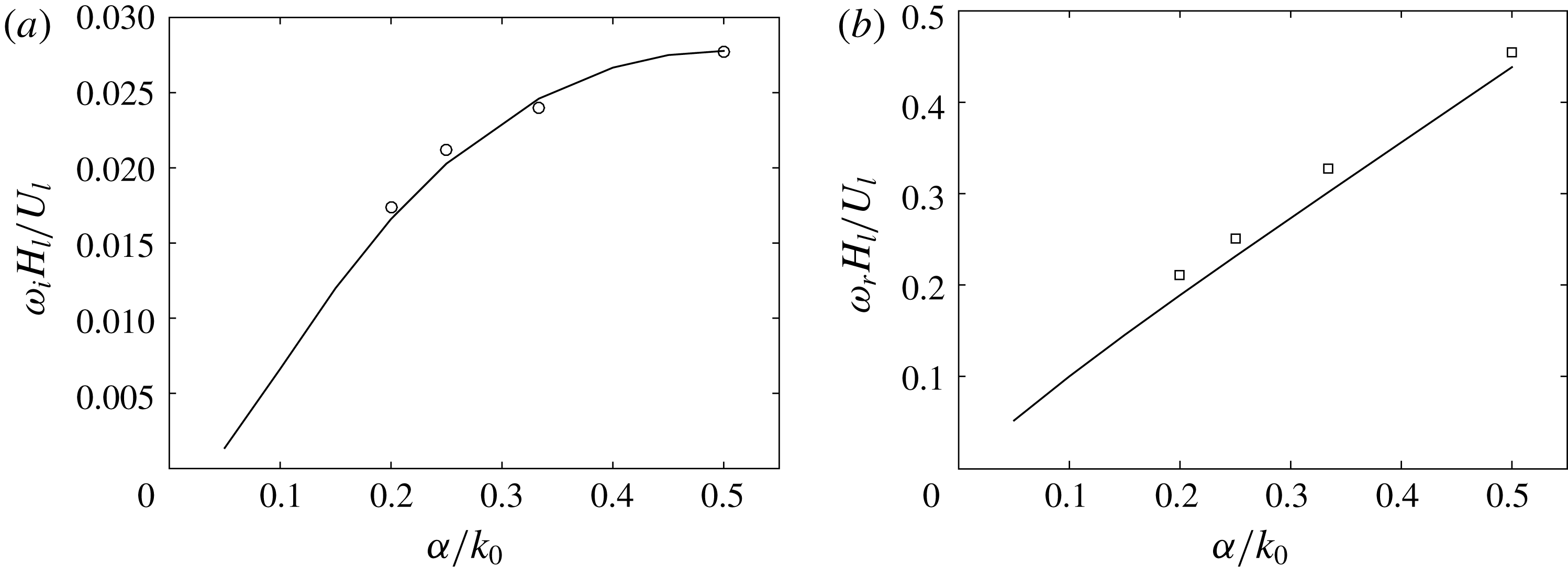
such that two waves exist in the same computational domain length. We compute the two-dimensional stability spectrum of this solitary wave, as plotted in figure 11. The stability analysis compares well with the direct numerical simulation of (2.6)–(2.7). We see that this solitary wave of
 $k_{0}$
is unstable to all the two-dimensional subharmonic disturbances with
 $\unicode[STIX]{x1D6FC}=0.5k_{0}$
growing fastest. Figure 12 shows the response of this solitary wave train to the most unstable two-dimensional perturbation
 $\unicode[STIX]{x1D6FC}=0.5k_{0}$
with a much smaller amplitude. The wave train initially appears to propagate steadily. As the subharmonic perturbation grows, the two waves gradually merge, eventually leaving a single solitary wave in the domain. This process is similar to figure 4(c) in the FCIF simulation even though it only includes a constant interfacial forcing. We thus interpret the wave coalescence in the two-way interaction problem as the analogue of the subharmonic instabilities of solitary waves.
(a) Typical computed growth rates of the most unstable two-dimensional disturbance of the periodic solitary waves of different steepness
 $k_{0}H_{l}$
with various
 $R_{f}$
for the one-way interaction problem. (b) The corresponding wavenumbers of the most unstable disturbance in (a). The results shown are for
 $R_{f}=4$
(○),
 $R_{f}=2$
(▫, blue) and
 $R_{f}=1$
(▿, red).

Two-dimensional stability results of the periodic solitary wave of
 $k_{0}H_{g}=0.2$
under constant interfacial forcing with
 $d=2$
in the one-way interaction problem. (a) Growth rate
 $\unicode[STIX]{x1D714}_{i}=\text{Im}(\unicode[STIX]{x1D70E})$
and (b) frequency
 $\unicode[STIX]{x1D714}_{r}=\text{Re}(\unicode[STIX]{x1D70E})+k_{0}c$
as a function of
 $\unicode[STIX]{x1D6FC}/k_{0}$
. Solid lines represent the results computed by the linear stability analysis, while symbols denote the results evaluated by direct spatio-temporal numerical simulation of (2.6)–(2.7).
(a) The eigenfunction corresponding to the most unstable two-dimensional disturbance of the periodic solitary wave of
 $k_{0}H_{g}=0.2$
with
 $d=2$
in the one-way interaction problem. The eigenfunction has been normalized so that its amplitude is
 $1/3$
times the crest-to-trough height of the unperturbed wave. The corresponding eigenvalue (i.e. complex frequency)
 $\unicode[STIX]{x1D70E}=0.00183i$
. (b) The unperturbed solitary wave profile (——) and the final solitary wave after coalescence for reference (– – –). (c) Spatio-temporal evolution of the interface with a small two-dimensional perturbation of
 $\unicode[STIX]{x1D6FC}=0.5k_{0}$
on the steady solitary wave in (a) by direct numerical simulation of (2.6)–(2.7).

Interfacial evolution through wave coalescence for the one-way interaction problem with
 $d=2$
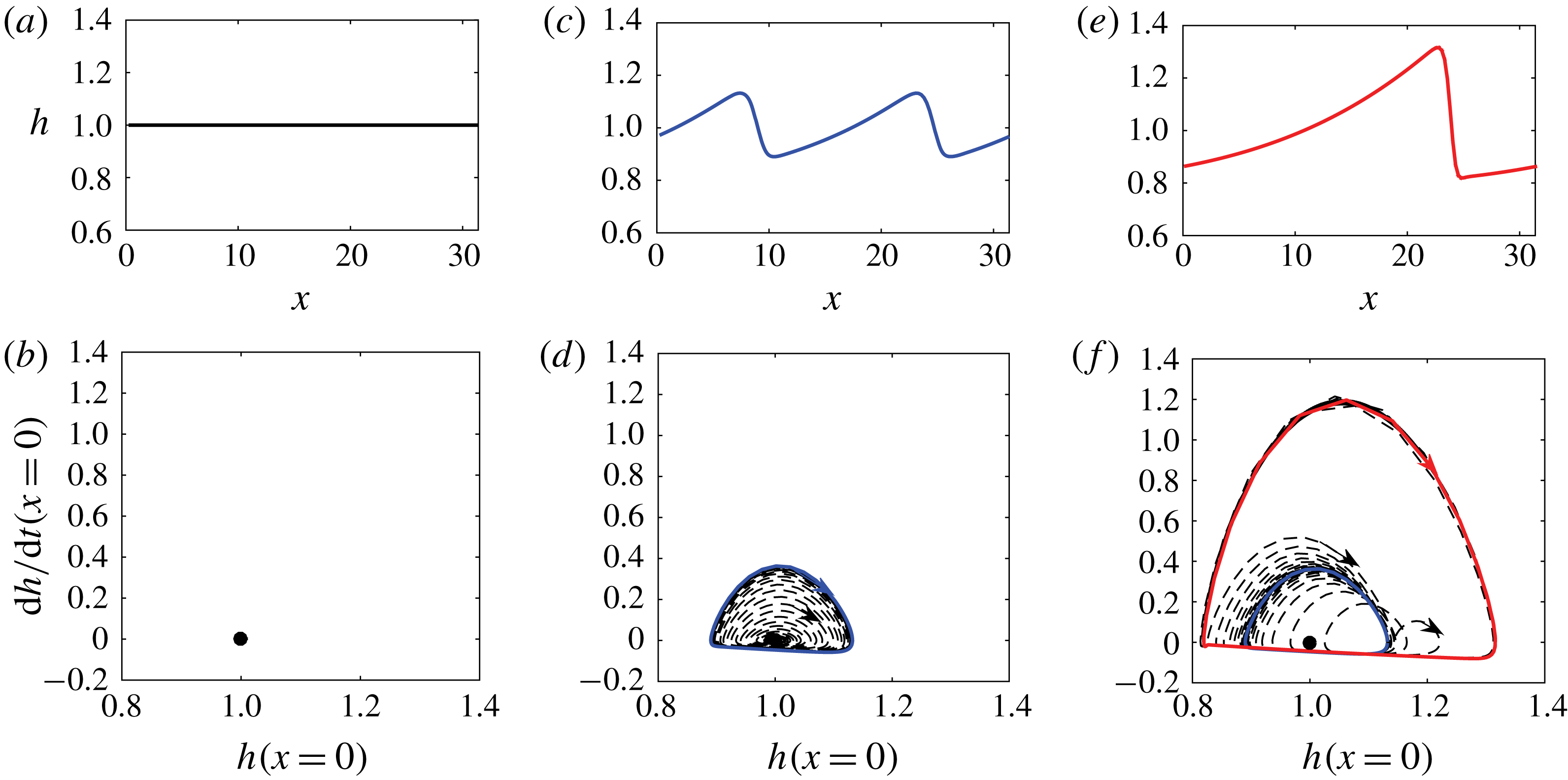
in the physical domain (a,c,e) and the corresponding phase plane (b,d,f). Solid lines and symbols represent different equilibria, whereas dashed lines denote phase plane trajectories.

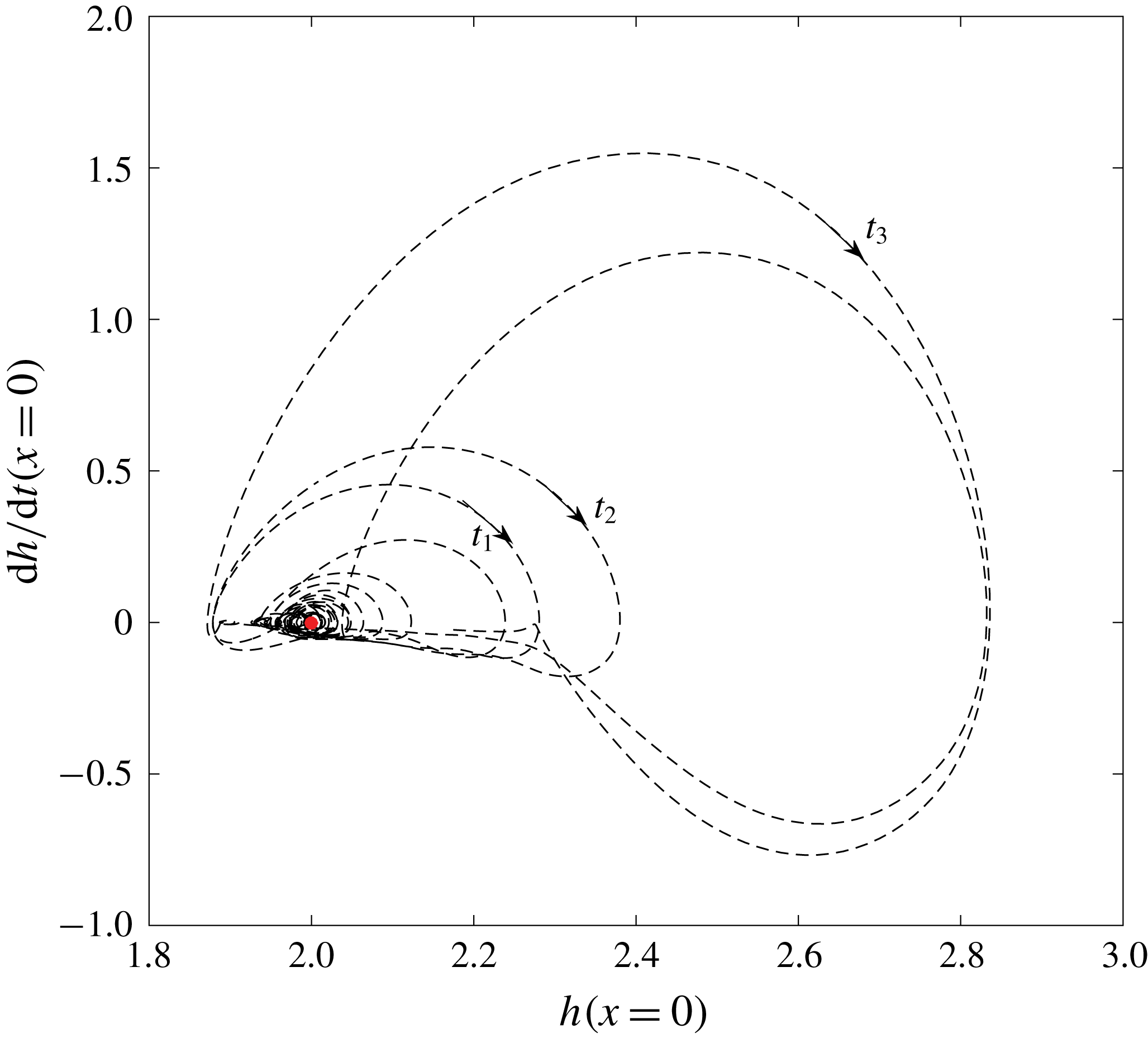
Phase plane trajectory (– – –) for the interfacial evolution in the two-way interaction problem by FCIF, where
 $t_{1}=130.2$
,
 $t_{2}=141.2$
and
 $t_{3}=238.5$
. Here ● (red) represents the flat interface equilibrium in the physical domain.

We summarize Process II from the perspective of dynamic theory. A laminar liquid flow driven by interfacial forcings is a nonlinear dynamic system allowing for multiple steady solutions. Process II is equivalent to successive bifurcations from these steady solutions. Take the one-way interaction problem as an example. The most trivial solution is the flat interface corresponding to an equilibrium point in the phase diagram (figure 13 a,b). Owing to linear interfacial instabilities, the system undergoes a Hopf bifurcation and gradually evolves from the flat interface into a periodic solitary wave that corresponds to a limit cycle in the phase diagram (figure 13 c,d). We have shown these solitary waves to be generally unstable to their subharmonic disturbances, so the system further bifurcates from the present limit cycle into a larger limit cycle in the phase plane (figure 13 f). This corresponds to forming a larger solitary wave through wave coalescence in the physical domain (figure 13 e). A series of such bifurcations result in slug generation. Figure 14 shows the similar characteristics in the phase plane trajectory of the FCIF simulation.
For the FCIF simulation, the wave grows to touch the channel top through wave coalescence after
 $t\sim 240$
. We estimate the slug-initiation distance utilizing the velocity of the largest wave (with
 $C_{g}=1.0$
) to be approximately 80 channel height from the inlet. This result compares qualitatively well in terms of time/length scale with the experimental observation of Andritsos et al. (Reference Andritsos, William and Hanratty1989) who reported that first slugging through wave coalescence occurred in the region of 30–100 pipe diameters for turbulent air and laminar liquid with viscosity of 20–
 $100cp$
(
 $Re_{l}\sim O(10)$
,
 $Re_{g}\sim O(10^{4})$
).
6 Influence of gas–liquid interactions on Processes I and II
We have shown the mechanism behind the growth of long waves through wave coalescence without invoking any complex interfacial force models. In fact, similar wave dynamics also exist in other wave systems such as one-layer falling thin films (e.g. Chang Reference Chang1994; Liu & Gollub Reference Liu and Gollub1994) and inclined open-channel shallow water flows (e.g. Kranenburg Reference Kranenburg1992; Balmforth & Mandre Reference Balmforth and Mandre2004). However, the energy sources for the interfacial instabilities are different. Gravity is the driving force for the falling thin films and inclined open-channel flows, while the fast gas flow is responsible for transferring energy to liquid via interfacial forces in two-layer flows. A constant interfacial pressure gradient in the latter is equivalent to the role of gravity in the former. In reality, the interfacial forcing is never constant in two-phase flows. Comparing figure 12 against figure 4(c), we find that wave coalescence takes much longer time in the one-way interaction problem and the resultant wave is smaller compared with the two-way interaction simulation. In this section, we show that with the two-way interaction between two phases included, the magnitude and phase correlation of the interfacial forces vary as waves evolve, which further accelerates the wave coalescence and wave growth.
6.1 Influence of interfacial waves on turbulent gas
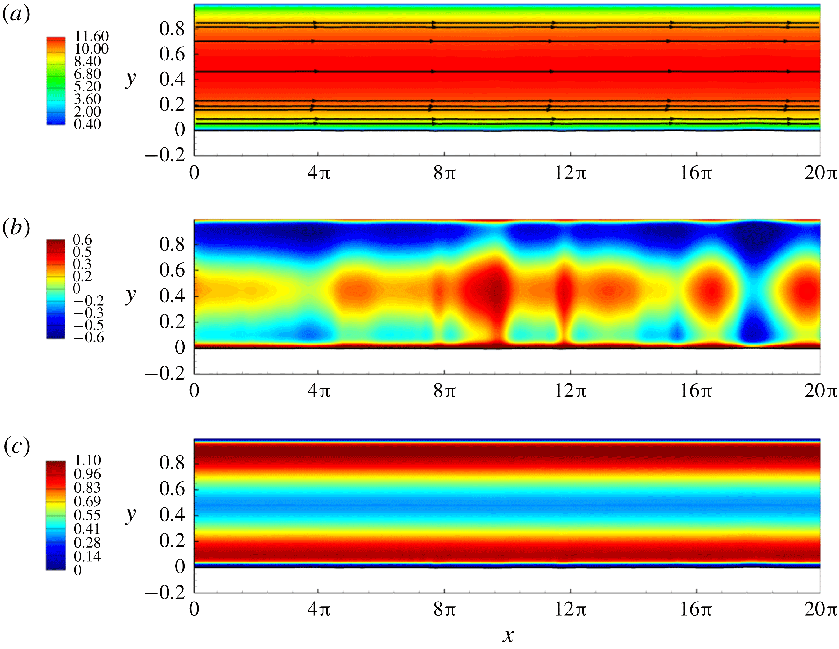
Snapshots of instantaneous contours of Reynolds-averaged velocity
 $u$
with mean streamlines by relative velocity
 $(u_{r}^{x},u_{r}^{y})=(u_{x}-u_{\unicode[STIX]{x1D702}}^{x},u_{y}-u_{\unicode[STIX]{x1D702}}^{y})$
, Reynolds-averaged pressure
 $p$
and TKE at
 $t=6$
in the early stage of the interfacial evolution leading to slugging in the turbulent-gas/laminar-liquid two-phase horizontal flow.

Snapshots of instantaneous contours of Reynolds-averaged velocity
 $u$
with mean streamlines by relative velocity
 $(u_{r}^{x},u_{r}^{y})=(u_{x}-u_{\unicode[STIX]{x1D702}}^{x},u_{y}-u_{\unicode[STIX]{x1D702}}^{y})$
, Reynolds-averaged pressure
 $p$
and TKE at
 $t=134$
in the later stage of the interfacial evolution leading to slugging in the turbulent-gas/laminar-liquid two-phase horizontal flow.

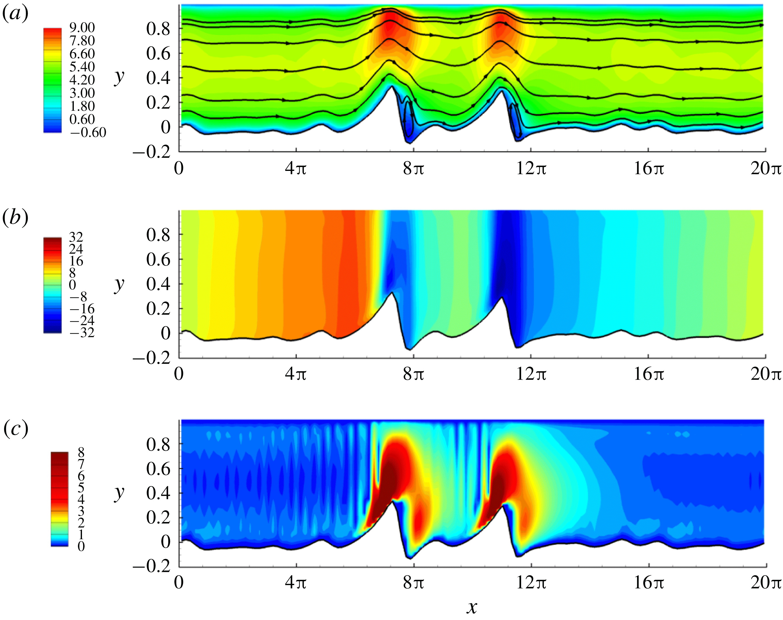
Figures 15 and 16 provide the gas flow visualization including the contours of Reynolds-averaged streamwise velocity
 $u$
, pressure
 $p$
and TKE for early (e.g.
 $t=6$
) and late (e.g.
 $t=134$
) stages, respectively. At the early stage when interfacial waves are small, the contours of
 $u$
,
 $p$
and TKE in the gas layer present a stratified pattern with perturbations due to small interfacial waves. The streamlines behave like a horizontally uniform flow. The turbulent stratified base flow dominates over the interfacial wave perturbations. However, once large interfacial waves are developed, the gas layer behaves similar to turbulent flow over hills and moving walls (Belcher & Hunt Reference Belcher and Hunt1998). The gas flow contours align with the interfacial waves, indicating that the influence of interfacial waves gradually dominates over the turbulent base flow as waves grow larger. In addition, the pressure drops rapidly at the two large wave crests due to the Bernoulli effect, but it does not immediately recover downstream of the crests where the effective gas cross-section widens. This means the viscosity effect is relevant at the later stage of slug generation. The closed streamlines (see figure 16
a) show that the flow separation occurs at the leeward side of the two large waves. This is consistent with the strong turbulence in the same region (see figure 16
c).
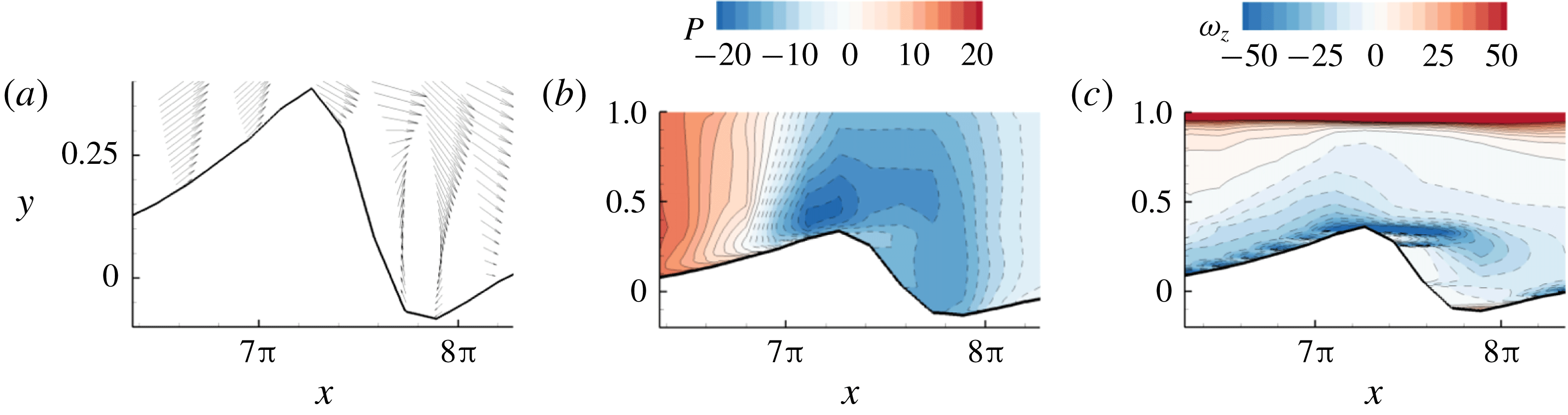
Figure 17 shows the flow separation details near the large solitary wave at
 $x=7\unicode[STIX]{x03C0}$
–
 $8\unicode[STIX]{x03C0}$
in figure 16, which is consistent with separated flows over hills/moving walls (Tobak & Peake Reference Tobak and Peake1982; Belcher & Hunt Reference Belcher and Hunt1998). The adverse pressure gradient downstream of the wave crest results in a locally reversed flow. The interfacial shear layer detaches the interface past the wave crest, shedding a large negative vortex into the flow. This is similar to the finding of Xie et al. (Reference Xie, Zheng, Triantafyllou, Constantinides, Zheng and Karniadakis2017) for the two-layer laminar flows in inclined channels that negative vorticity mostly results from the interface. The flow separation due to the large interfacial waves at the later stage thickens the boundary layer on the leeward side of the wave, thereby displacing the outer mean flow asymmetrically about the wave. This explains the slow recovery of the pressure downstream of the crests shown in figure 16(b), which is also consistent with the sheltering hypothesis of Jeffreys (Reference Jeffreys1925). We further discuss this asymmetry of the pressure distribution in § 6.3.
(a) The relative velocity vector field
 $(u_{r}^{x},u_{r}^{y})=(u_{x}-u_{\unicode[STIX]{x1D702}}^{x},u_{y}-u_{\unicode[STIX]{x1D702}}^{y})$
, (b) the detailed mean pressure contour and (c) the mean vorticity contour near the large wave at
 $x=7\unicode[STIX]{x03C0}$
–
 $8\unicode[STIX]{x03C0}$
and
 $t=134$
(see figure 16). The dashed contour lines denote negative values.

6.2 Influence of turbulent gas on interfacial pressure-to-shear strength ratio
Comparisons of wave-induced interfacial pressure gradient
 $\unicode[STIX]{x0394}(-\text{d}p_{\unicode[STIX]{x1D702}}/\text{d}x)$
, interfacial shear stress
 $\unicode[STIX]{x1D70F}_{\unicode[STIX]{x1D702}}^{x}$
and wave elevation
 $\unicode[STIX]{x1D702}$
profiles at
 $t=6$
in the early stage (a–c), and
 $t=134$
in the late stage (d–f) of the interfacial evolution leading to slugging in laminar liquid sheared by turbulent gas in horizontal channels. Dashed lines (– – –) represent the profiles in the base flow for reference.

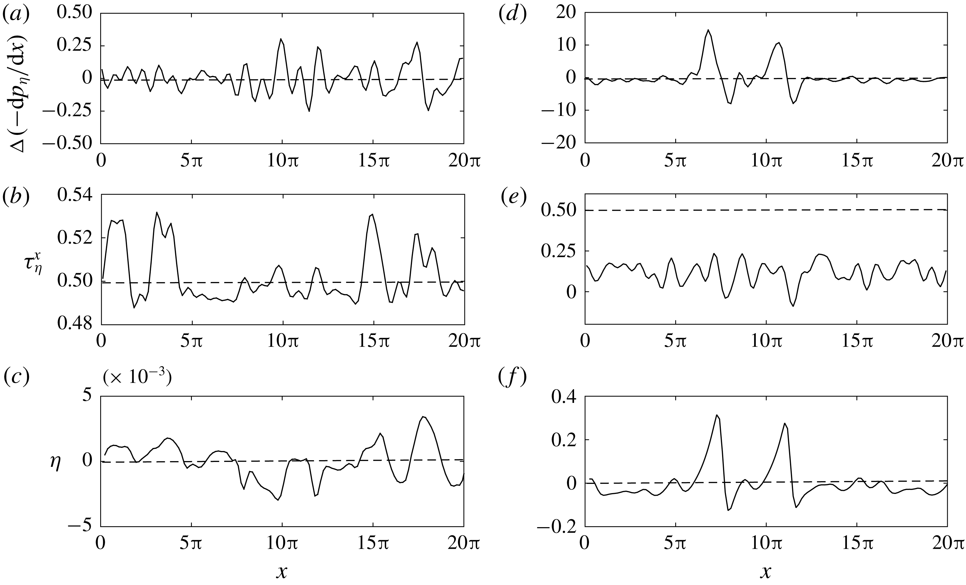
The evolving influence of interfacial waves on the turbulent gas layer would in return influence the interfacial forces driving the liquid motion. Figure 18 shows two representative profiles of the wave-induced interfacial pressure drop
 $\unicode[STIX]{x0394}(-\text{d}p_{\unicode[STIX]{x1D702}}/\text{d}x)=(-\text{d}p_{\unicode[STIX]{x1D702}}/\text{d}x)-P_{x}$
and interfacial shear stress
 $\unicode[STIX]{x1D70F}_{\unicode[STIX]{x1D702}}^{x}$
at early and late stages, respectively. At the early stage, the leading order of the flow is the stratified base flow. The magnitude of the wave-induced pressure drop
 $\unicode[STIX]{x0394}(-\text{d}p_{\unicode[STIX]{x1D702}}/\text{d}x)$
is small compared with the applied pressure drop
 $P_{x}$
. At the later stage with much larger interfacial waves,
 $\unicode[STIX]{x0394}(-\text{d}p_{\unicode[STIX]{x1D702}}/\text{d}x)$
completely dominates over
 $P_{x}$
. The magnitude of the interfacial shear stress at the later stage is also much smaller than that at the initial stage. The shear stress may turn into drag force where flow separation occurs. Compared with the interfacial pressure, the shear stress effect at the later stage is negligible.
Time evolution of interfacial pressure-to-shear strength ratio
 $R_{f}(t)$
during slug generation in the two-phase turbulent-gas/laminar-liquid horizontal flow.

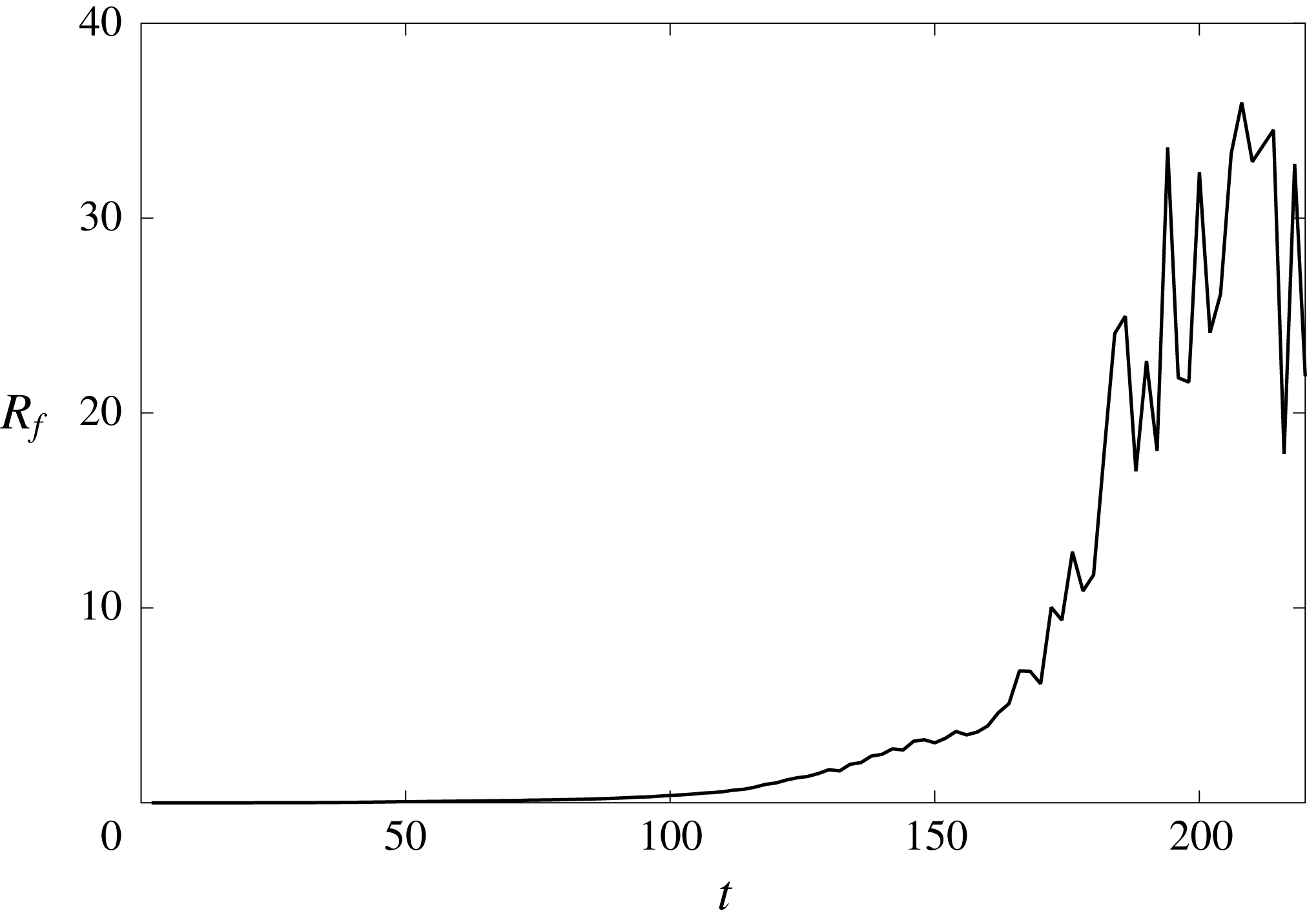
To quantify the strength ratio between interfacial pressure and shear stress during the slug-generation process, we define the following metric similar to (5.2):
 $$\begin{eqnarray}R_{f}(t)=\frac{\left\langle -{\displaystyle \frac{\text{d}p_{\unicode[STIX]{x1D702}}}{\text{d}x}}h\right\rangle }{\langle \unicode[STIX]{x1D70F}_{\unicode[STIX]{x1D702}}^{x}\rangle },\end{eqnarray}$$
where
 $\langle a\rangle =\int a\,\text{d}x/\int \text{d}x$
denotes the space average of quantity
 $a$
. We compute the time variation of
 $R_{f}(t)$
during the entire slug generation, which is displayed in figure 19. We observe a monotonic increase of
 $R_{f}$
throughout the slug development. It is clear from § 5 that larger pressure-to-shear ratio tends to form larger faster solitary waves (see figure 7) and produce stronger subharmonic instabilities (see figure 10). Thus, the increase of
 $R_{f}(t)$
with time indicates that the dynamic interaction between gas and liquid further accelerates the wave coalescence and facilitates the formation of larger longer solitary waves.
Energy flux from turbulent gas to laminar liquid through interfacial forces during the slug-generation process: – – –, through
 $p_{\unicode[STIX]{x1D702}}$
; —
 $\cdot$
—, through
 $\unicode[STIX]{x1D70F}_{\unicode[STIX]{x1D702}}^{x}$
; ——, total energy flux.

The evolution of interfacial pressure-to-shear strength ratio in the two-layer flow also results in the energy source for interfacial wave growth differing from many one-layer wave systems driven by a constant force (e.g. gravity). Figure 20 shows the gas-to-liquid energy flux during the slug development. The dynamic interaction between gas and liquid results in a more rapid energy transfer rate in the later stage, indicating an increasing interfacial wave growth rate as the waves grow. The energy transfer is initially by interfacial shear stress and then ultimately by interfacial pressure forcing. This is consistent with the evolution of
 $R_{f}$
in figure 19.
6.3 Influence of turbulent gas on the phase correlation of the interfacial pressure gradient
The wave-affected turbulent gas also influences the phase distribution of the interfacial pressure in addition to its magnitude throughout the interfacial evolution towards slugging. From figure 18(d,f), we see that both Bernoulli (KH) and viscous effects due to the gas–liquid interaction influence the interfacial pressure distribution. The pressure drop upstream of the wave crests is positive due to the acceleration of the gas flow induced by the reduction in the cross-sectional area (Bernoulli effect). Conversely, the pressure drop is negative downstream of the wave crests. Such a pressure distribution drives the liquid from troughs to crest, elevating the interface similar to the KH instability. The asymmetry (with respect to the wave crest) of the boundary layer thickness due to the flow separation at the lee side of the large waves (figures 16 and 17) modifies the symmetry of the interfacial pressure gradient. This viscous effect attenuates the interfacial pressure gradient downstream of the wave, resulting in a larger net driving force on larger waves. This helps precipitate the wave coalescence as displayed in figure 3. Overall, these two effects result in a strong correlation between interfacial pressure gradient and wave elevation at
 $t=134$
, which was weak at
 $t=6$
(figure 18
a,c).
There has been a debate on the phase correlation of the interfacial pressure with the wave elevation (e.g. KH model) and wave slope (e.g. Jeffreys’ sheltering mechanism) for two-phase flows (e.g. Hanratty & Engen Reference Hanratty and Engen1957; Cohen & Hanratty Reference Cohen and Hanratty1965; Campbell et al.
Reference Campbell, Hendrickson and Liu2016). We compute the correlation coefficient of the interfacial pressure drop
 $-\text{d}p_{\unicode[STIX]{x1D702}}/\text{d}x$
with both wave elevation
 $\unicode[STIX]{x1D702}$
and wave slope
 $-\text{d}\unicode[STIX]{x1D702}/\text{d}x$
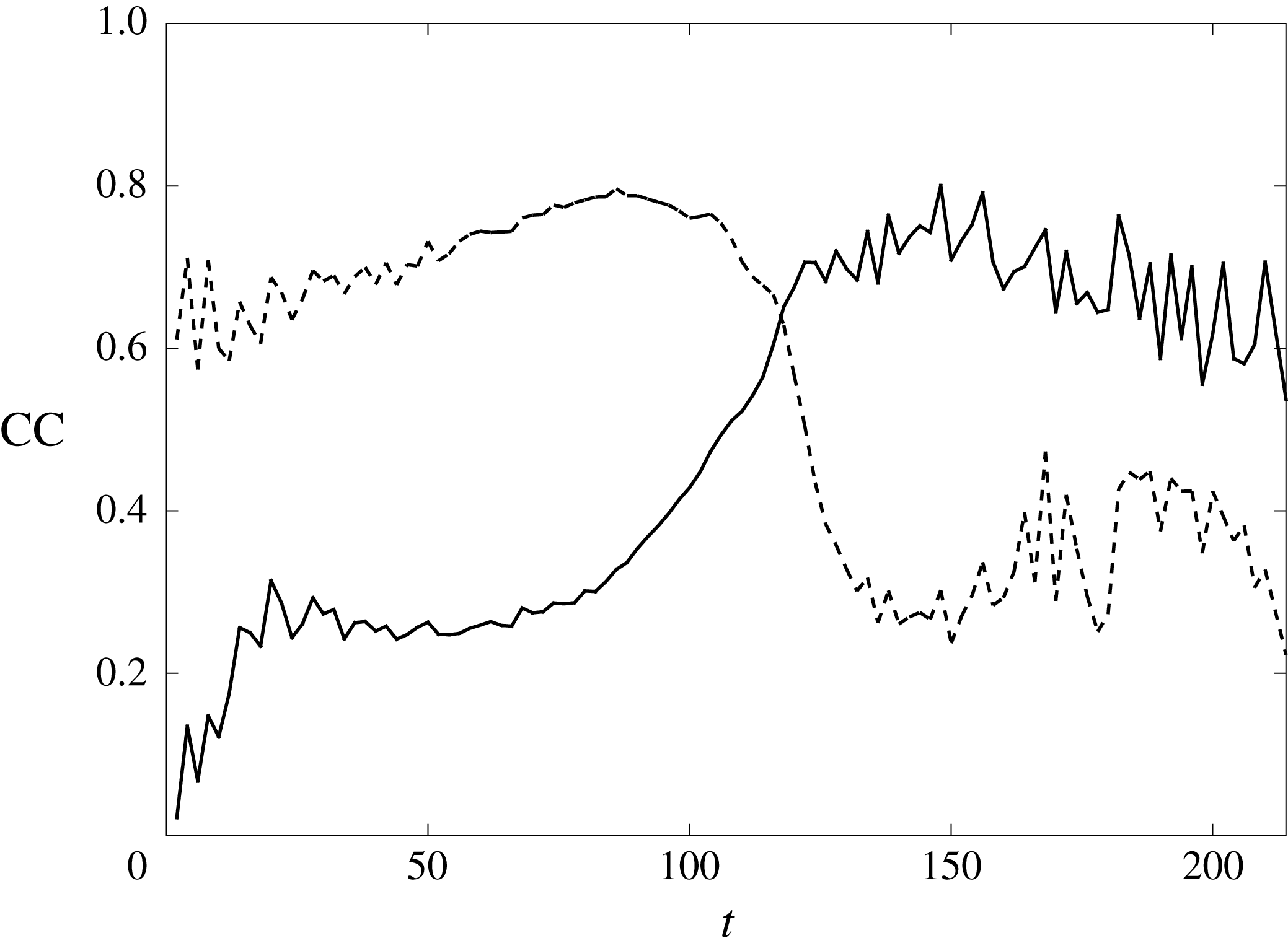
during the slug development, as shown in figure 21. We see a transition point at around
 $t=100{-}120$
. The interfacial pressure gradient correlates dominantly first with wave slope and then with elevation.
Evolution of correlation coefficients (CC) of interfacial pressure gradient
 $-\text{d}p_{\unicode[STIX]{x1D702}}/\text{d}x$
with wave elevation
 $\unicode[STIX]{x1D702}$
(——), and with elevation slope
 $\text{d}\unicode[STIX]{x1D702}/\text{d}x$
(– – –).

This correlation evolution is a result of the competition between Bernoulli (KH) and viscous effects as waves grow. For an unbounded turbulent flow over one wavy wall, such a competition exists depending on the strength of the boundary effect in different flow regions (Belcher & Hunt Reference Belcher and Hunt1998). The perturbed horizontal pressure drop is mainly balanced with the perturbed shear stress gradient in the inner (local-equilibrium) region (Townsend Reference Townsend1961), while it is determined by the Bernoulli effect in the outer (rapid-distortion) region (Batchelor & Proudman Reference Batchelor and Proudman1954; Hunt Reference Hunt1973). Similarly, the turbulent gas layer during the slug generation is a bounded flow between two walls gradually approaching each other because the gas sees the liquid as a moving wall. The bulk region of the gas flow thus gradually transitions from outer (rapid-distortion) to inner (local-equilibrium) region as waves approach the channel top. Therefore, the perturbed pressure gradient initially balances with the wave-induced convection term (Bernoulli/KH effect) and then with shear stress gradient (viscous effect), resulting in the phase-correlation evolution.
In summary, the two-way interaction between the bounded turbulent gas and laminar liquid further accelerates the wave growth and coalescence in slug generation by increasing the interfacial pressure-to-shear strength ratio and changing the phase correlation of interfacial pressure gradient. The interfacial pressure gradient initially correlates with wave slope to destabilize the interface as the KH instability due to the Bernoulli effect. In the later stage, it correlates with wave elevation due to a stronger stress gradient effect competing over the Bernoulli effect in a wave-influenced turbulent gas layer in a bounded domain, which tends to drive larger waves to travel faster for wave coalescence and growth.
7 Process III: slugging
Through the initial linear instabilities and the subsequent nonlinear coalescence, interfacial waves grow larger and longer such that they approach the top channel wall leading to rapid slugging. In this section, we perform a short-time asymptotic analysis on this final stage of slug formation when waves are close to bridging the channel, i.e. when
 $H-h\ll 1$
, where
 $H$
is the total channel height and
 $h$
is the interfacial wave height.
7.1 Reduced model
The gas layer transfers energy to liquid mainly through interfacial pressure in the later stage. To describe the dynamics of the interface in the last stage, we first perform a control volume analysis for the turbulent gas layer to model the interfacial pressure gradient. Within the context of two-dimensional problems, we select a control volume covering the cross-section of the gas layer and spanning from
 $x$
to
 $x+\text{d}x$
for
 $\text{d}x\rightarrow 0$
, with the top wall and the interface as the top and bottom boundaries, respectively. From the mass conservation, we obtain
 $$\begin{eqnarray}\frac{\unicode[STIX]{x2202}(H-h)}{\unicode[STIX]{x2202}t}+\frac{\unicode[STIX]{x2202}Q_{x}}{\unicode[STIX]{x2202}x}=0,\end{eqnarray}$$
where
 $Q_{x}$
is the gas flow rate:
 $$\begin{eqnarray}Q_{x}=\int _{h}^{H}u\,\text{d}y.\end{eqnarray}$$
Combining (7.1) with (2.6)–(2.7) yields
 $$\begin{eqnarray}Q_{x}+q_{x}={\mathcal{Q}}(t),\end{eqnarray}$$
and here we focus on the case of constant total flow rate,
 ${\mathcal{Q}}(t)\equiv {\mathcal{Q}}$
. In general, gas travels much faster than liquid, thus we assume the gas layer is in a quasi-steady state (Taitel & Dukler Reference Taitel and Dukler1976; Lin & Hanratty Reference Lin and Hanratty1986). Then the momentum conservation of the control volume yields
 $$\begin{eqnarray}\frac{\unicode[STIX]{x2202}}{\unicode[STIX]{x2202}x}\int _{h}^{H}u^{2}\,\text{d}y=-(H-h)\frac{\text{d}p_{\unicode[STIX]{x1D702}}}{\text{d}x}-(\unicode[STIX]{x1D70F}_{H}^{x}+\unicode[STIX]{x1D70F}_{\unicode[STIX]{x1D702}}^{x}).\end{eqnarray}$$
 $$\begin{eqnarray}-\frac{\text{d}p_{\unicode[STIX]{x1D702}}}{\text{d}x}=\unicode[STIX]{x1D6F7}\frac{\unicode[STIX]{x2202}}{\unicode[STIX]{x2202}x}\left[\frac{{\mathcal{Q}}-q_{x}}{H-h}\right]^{2}+\frac{\unicode[STIX]{x1D70F}_{H}^{x}+\unicode[STIX]{x1D70F}_{\unicode[STIX]{x1D702}}^{x}}{H-h},\end{eqnarray}$$
where
 $\unicode[STIX]{x1D6F7}$
is the shape factor defined as (Lin & Hanratty Reference Lin and Hanratty1986)
 $$\begin{eqnarray}\unicode[STIX]{x1D6F7}=\frac{H-h}{({\mathcal{Q}}-q_{x})^{2}}\int _{h}^{H}u^{2}\,\text{d}y.\end{eqnarray}$$
The value of
 $\unicode[STIX]{x1D6F7}$
depends on the mean flow velocity profile and here we choose
 $\unicode[STIX]{x1D6F7}=1$
(Balmforth & Mandre Reference Balmforth and Mandre2004).
We calculate the stress gradient term in the right-hand side of (7.5) using the expression
 $$\begin{eqnarray}\frac{\unicode[STIX]{x1D70F}_{H}^{x}+\unicode[STIX]{x1D70F}_{\unicode[STIX]{x1D702}}^{x}}{H-h}=I^{2}\left(\frac{{\mathcal{Q}}-q_{x}}{H-h}\right)^{2},\end{eqnarray}$$
where
 $I$
represents the turbulence intensity modelled by the following Blasius-type power law correlation (Taitel & Dukler Reference Taitel and Dukler1976; Andritsos & Hanratty Reference Andritsos and Hanratty1987a
; Spedding & Hand Reference Spedding and Hand1997; Issa & Kempf Reference Issa and Kempf2003):
 $$\begin{eqnarray}I=aRe_{g}^{-b}=a\left[\frac{\unicode[STIX]{x1D70C}_{g}({\mathcal{Q}}-q_{x})}{\unicode[STIX]{x1D707}_{g}}\right]^{-b},\end{eqnarray}$$
where
 $a$
and
 $b$
are unknown coefficients to be determined by the specific problem.
Substituting equations (7.7)–(7.8) into (7.5), we obtain the following model for interfacial pressure gradient:
 $$\begin{eqnarray}-\frac{\text{d}p_{\unicode[STIX]{x1D702}}}{\text{d}x}=\frac{\unicode[STIX]{x2202}}{\unicode[STIX]{x2202}x}\left[\frac{{\mathcal{Q}}-q_{x}}{H-h}\right]^{2}+a\left(\frac{\unicode[STIX]{x1D70C}_{g}}{\unicode[STIX]{x1D707}_{g}}\right)^{-b}\frac{({\mathcal{Q}}-q_{x})^{-b+2}}{(H-h)^{3}}.\end{eqnarray}$$
For
 $H-h\ll 1$
, the second term on the right-hand side dominates, consistent with the inner (local-equilibrium) region behaviour of the whole gas layer at the later stage of slug generation (see § 6.3). By neglecting the first term on the right-hand side, we substitute the interfacial pressure gradient model (7.9) into (2.6)–(2.7). The dominance of the pressure term for
 $H-h\ll 1$
allows us to further neglect all the other forcing terms, yielding the following reduced equations describing the rapid growth of interfacial waves in Process III:
 $$\begin{eqnarray}\displaystyle & \displaystyle \frac{\unicode[STIX]{x2202}h}{\unicode[STIX]{x2202}t}+\frac{\unicode[STIX]{x2202}q_{x}}{\unicode[STIX]{x2202}x}=0 & \displaystyle\end{eqnarray}$$
 $$\begin{eqnarray}\displaystyle & \displaystyle \frac{\unicode[STIX]{x2202}q_{x}}{\unicode[STIX]{x2202}t}+\frac{6}{5}\frac{\unicode[STIX]{x2202}}{\unicode[STIX]{x2202}x}\left(\frac{q_{x}^{2}}{h}\right)=ra\left(\frac{\unicode[STIX]{x1D70C}_{g}}{\unicode[STIX]{x1D707}_{g}}\right)^{-b}\frac{({\mathcal{Q}}-q_{x})^{-b+2}}{(H-h)^{3}}h. & \displaystyle\end{eqnarray}$$
7.2 Asymptotic results
We perform an asymptotic analysis on the final slugging event in Process III for the turbulent-gas/laminar-liquid horizontal two-phase flow. We determine
 $a$
and
 $b$
of the interfacial pressure gradient model (7.9) using the distributions of
 $\text{d}p_{\unicode[STIX]{x1D702}}/\text{d}x$
at different time instants throughout Process I and II from the FCIF simulation. We randomly choose multiple sets of
 $\text{d}p_{\unicode[STIX]{x1D702}}/\text{d}x$
from the FCIF simulation results to combine into a training set. The remaining data then form a test set. Using the power regression with the training set obtains
 $a=4.752\times 10^{-3}$
,
 $b=-1.618$
, which are also validated by the test set. Figure 22 provides several sample comparisons between the interfacial pressure model and the numerical simulation results by FCIF for the test datasets throughout Process I and II. The comparison is satisfactory.
Comparisons of the interfacial pressure gradient distributions
 $\text{d}p_{\unicode[STIX]{x1D702}}/\text{d}x$
between the numerical simulation by FCIF (——) and the interfacial pressure model (7.9) with
 $a=4.752\times 10^{-3}$
,
 $b=-1.618$
(– – –) at (a)
 $t=30$
, (b)
 $t=80$
, (c)
 $t=150$
and (d)
 $t=240$
in the slug-generation process of turbulent-gas/laminar-liquid two-phase horizontal flow.

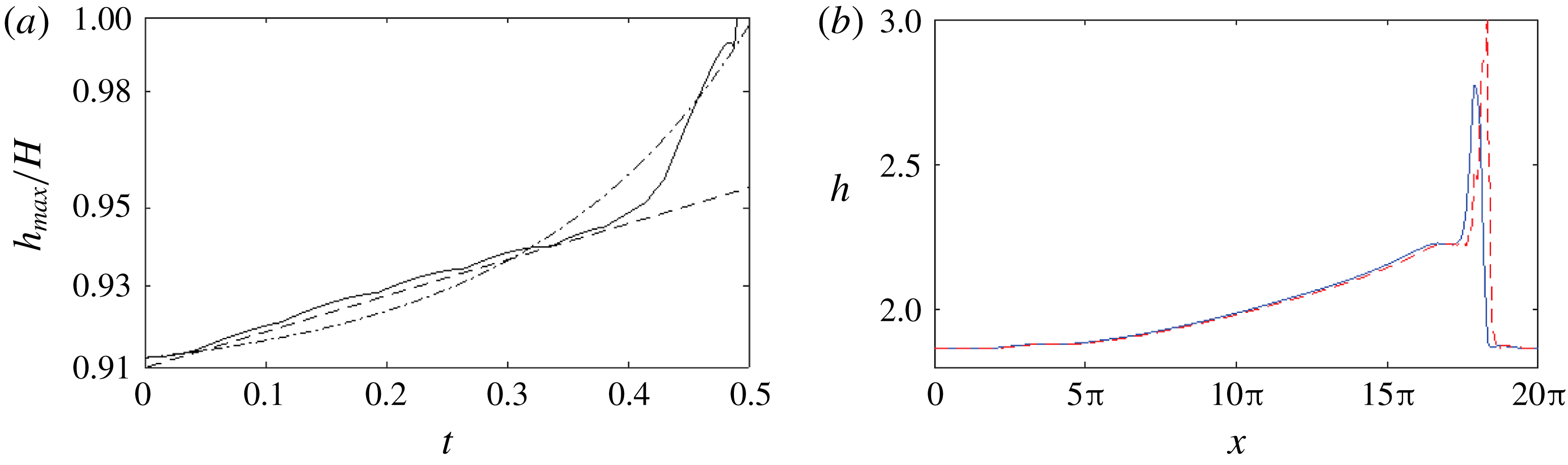
(a) Growth of the wave crest (——) in Process III when the wave nears the top wall for the turbulent-gas/laminar-liquid two-phase flow. Here – – – and —
 $\cdot$
— represent exponential and tri-exponential functions, respectively. (b) The corresponding elevation profiles at the beginning (
 $t_{0}=240$
) (——, blue) and the end (
 $t=t_{0}+0.5$
) (– – –, red) of Process III immediately before slugging.

Once
 $a$
and
 $b$
are determined, we numerically solve the governing equations (7.10) of Process III using the quasi-steady solitary wave at
 $t=240$
as the initial condition. Figure 23 shows the asymptotic behaviour of the wave growth right before slugging occurs. We see that when the wave nears the top channel wall, it achieves faster than exponential, or even tri-exponential growth rate until bridging the channel to form a slug. The characteristic feature of rapid approach of the interface to the top wall in the occurrence of slugging is consistent with the experimental observation (e.g. figure 6 in Kadri et al.
Reference Kadri, Mudde, Oliemans, Bonizzi and Andreussi2009).
8 Conclusion
This work has numerically and theoretically investigated the mechanisms of slug generation for a two-phase turbulent-gas/laminar-liquid flow in a horizontal channel using a newly developed FCIF solver combined with interfacial instability analyses. FCIF couples a uRANS gas simulator with a depth-integrated (long-wave) liquid solver via an IB method to efficiently simulate the dynamic interaction between two disparate flows on a single non-boundary conforming grid. The analyses of numerical simulations by FCIF and interfacial instabilities and comparisons with available experimental observations have shown that the slugs develop from stratified two-phase flows through three fundamental cascaded processes. This paper has detailed the characteristics of the dynamics and the associated governing mechanisms associated with the three processes.
Process I is the growth of minuscule waves on the flat interface. We have performed a TOS analysis, based on the QL hypothesis, of the Poiseuille base flow and have shown that the base flow is linearly unstable for the long Fourier wave modes of disturbances. The numerical simulation by FCIF confirms that the linear OS instability causes the stratified-to-wavy transition in Process I.
Process II is the formation and coalescence of long solitary waves evolved from relatively shorter waves induced by linear instability in Process I. To assist in understanding the mechanisms behind this process, we first consider a relatively simple problem by neglecting the influence of interfacial waves on turbulent gas. By performing wave spectrum and normal-mode perturbation analyses for this one-way coupling problem, we show that nonlinear solitary waves, which result from multiple resonant and/or near-resonant triad (or higher-order) interactions of weakly dispersive Fourier modes (from the initial linear instability in Process I), coalesce due to the instabilities to their subharmonic disturbances. This mechanism results in a continuous coalescence of solitary waves to produce waves of increasing size (in both wavelength and wave amplitude), eventually leading to slugging. We then investigate the influence of two-way interaction of turbulent gas and laminar liquid flows on this nonlinear interfacial wave evolution process. Examination on interfacial force variations in the two-way coupling simulation indicates that the gas–liquid interaction precipitates the wave growth and coalescence, further accelerating the slug generation.
Finally, through the linear instabilities in Process I and nonlinear coalescence in Process II, Process III is the rapid wave growth immediately before bridging the channel. By developing a reduced physical model and performing an asymptotic analysis on the wave behaviour as waves approach the channel top, we find that waves could achieve multiple-exponential growth (with time) before hitting the channel top to initiate slugging. This is mechanically consistent with the observation of high-impact pressure/force on pipe/channel wall when a slug forms.
Together, the analysis of these three fundamental processes provides a comprehensive understanding on the entire slug generation from a stratified flow regime in horizontal turbulent-gas/laminar-liquid two-phase flows. Our mechanistic study provides important insights and guidance for developing interfacial force closure models, predicting slug transition criteria, and estimating slug frequency/length. The FCIF simulations and three-dimensional stability analysis presented here (as well as the simulations of Xie et al. Reference Xie, Zheng, Triantafyllou, Constantinides, Zheng and Karniadakis2017) establish the dominant mechanism for wave coalescence and the onset of slugging as mainly a two-dimensional mechanism. The interfacial evolution of the FCIF simulations is also characteristically similar to those observed in the pipe experiments (e.g. Andritsos et al. Reference Andritsos, William and Hanratty1989; Fan et al. Reference Fan, Lusseyran and Hanratty1993; Woods & Hanratty Reference Woods and Hanratty1999) and three-dimensional simulations (e.g. Issa & Kempf Reference Issa and Kempf2003; Frank Reference Frank2005; Höhne & Mehlhoop Reference Höhne and Mehlhoop2014). We expect the details of pipe curvature and three-dimensional turbulence structures to have an influence on the rate at which the process occurs; however, we do not expect it to significantly alter the underlying two-dimensional mechanisms driving the phenomenon.
Acknowledgement
This work was supported by the Chevron Corporation and the Office of Naval Research (N00014-15-1-2460 and N00014-17-1-2089). Their sponsorship is greatly appreciated.
Appendix A. Three-dimensional instability analysis of periodic solitary waves
In this appendix, we study the instability of a two-dimensional periodic solitary wave of
 $k_{0}$
derived for the one-way interaction problem in § 5.1. Consider the solitary wave subject to an infinitesimal three-dimensional disturbance. In a frame of reference moving with the wave speed
 $c$
, let
 $$\begin{eqnarray}h=h_{0}(x)+h^{\prime },\quad q_{x}=q_{x}^{0}(x)+q_{x}^{\prime },\quad q_{z}=q_{z}^{\prime },\end{eqnarray}$$
where
 $h_{0}$
and
 $q_{x}^{0}$
are the elevation and flow rate profiles of the base solitary wave, and
 $h^{\prime }\ll h_{0}$
and
 $q_{x}^{\prime },q_{z}^{\prime }\ll q_{x}^{0}$
are small perturbations. To first order in the perturbations, from (5.3)–(5.5) we obtain
 $$\begin{eqnarray}\frac{\unicode[STIX]{x2202}h^{\prime }}{\unicode[STIX]{x2202}t}-c\frac{\unicode[STIX]{x2202}h^{\prime }}{\unicode[STIX]{x2202}x}+\frac{\unicode[STIX]{x2202}q_{x}^{\prime }}{\unicode[STIX]{x2202}x}+\frac{\unicode[STIX]{x2202}q_{z}^{\prime }}{\unicode[STIX]{x2202}z}=0,\end{eqnarray}$$
 $$\begin{eqnarray}\displaystyle \frac{\unicode[STIX]{x2202}q_{x}^{\prime }}{\unicode[STIX]{x2202}t}+{\mathcal{A}}h^{\prime }+{\mathcal{B}}\frac{\unicode[STIX]{x2202}h^{\prime }}{\unicode[STIX]{x2202}x}+{\mathcal{C}}q_{x}^{\prime }+{\mathcal{D}}\frac{\unicode[STIX]{x2202}q_{x}^{\prime }}{\unicode[STIX]{x2202}x}+({\mathcal{I}}+c)\frac{\unicode[STIX]{x2202}q_{z}^{\prime }}{\unicode[STIX]{x2202}z} & = & \displaystyle \frac{1}{Re_{l}}\left[2\frac{\unicode[STIX]{x2202}^{2}q_{x}^{\prime }}{\unicode[STIX]{x2202}x^{2}}+\frac{\unicode[STIX]{x2202}^{2}q_{x}^{\prime }}{\unicode[STIX]{x2202}z^{2}}+\frac{\unicode[STIX]{x2202}^{2}q_{z}^{\prime }}{\unicode[STIX]{x2202}x\unicode[STIX]{x2202}z}\right]\nonumber\\ \displaystyle & & \displaystyle +\,We_{l}h_{0}\left[\frac{\unicode[STIX]{x2202}^{3}h^{\prime }}{\unicode[STIX]{x2202}x^{3}}+\frac{\unicode[STIX]{x2202}^{3}h^{\prime }}{\unicode[STIX]{x2202}x\unicode[STIX]{x2202}z^{2}}\right],\end{eqnarray}$$
 $$\begin{eqnarray}\displaystyle \frac{\unicode[STIX]{x2202}q_{z}^{\prime }}{\unicode[STIX]{x2202}t}+\frac{h_{0}}{Fr_{l}^{2}}\frac{\unicode[STIX]{x2202}h^{\prime }}{\unicode[STIX]{x2202}z}+{\mathcal{G}}q_{z}^{\prime }+{\mathcal{I}}\frac{\unicode[STIX]{x2202}q_{z}^{\prime }}{\unicode[STIX]{x2202}x} & = & \displaystyle \frac{1}{Re_{l}}\left[\frac{\unicode[STIX]{x2202}^{2}q_{z}^{\prime }}{\unicode[STIX]{x2202}x^{2}}+\frac{2\unicode[STIX]{x2202}^{2}q_{z}^{\prime }}{\unicode[STIX]{x2202}z^{2}}+\frac{\unicode[STIX]{x2202}^{2}q_{z}^{\prime }}{\unicode[STIX]{x2202}x\unicode[STIX]{x2202}z}\right]\nonumber\\ \displaystyle & & \displaystyle +\,We_{l}h_{0}\left[\frac{\unicode[STIX]{x2202}^{3}h^{\prime }}{\unicode[STIX]{x2202}z^{3}}+\frac{\unicode[STIX]{x2202}^{3}h^{\prime }}{\unicode[STIX]{x2202}x^{2}\unicode[STIX]{x2202}z}\right],\end{eqnarray}$$
where
 $$\begin{eqnarray}\displaystyle {\mathcal{A}} & = & \displaystyle -\frac{6}{5}\frac{\unicode[STIX]{x2202}}{\unicode[STIX]{x2202}x}\left(\frac{q_{x}^{0}}{h_{0}}\right)^{2}+\frac{1}{5}\unicode[STIX]{x1D70F}_{\unicode[STIX]{x1D702}}^{x}\unicode[STIX]{x1D6E4}^{x}h_{0}^{2}\frac{\unicode[STIX]{x2202}h_{0}}{\unicode[STIX]{x2202}x}+\frac{1}{5}(\unicode[STIX]{x1D70F}_{\unicode[STIX]{x1D702}}^{x})^{2}h_{0}\frac{\unicode[STIX]{x2202}h_{0}}{\unicode[STIX]{x2202}x}\end{eqnarray}$$
 $$\begin{eqnarray}\displaystyle & & \displaystyle +\,\frac{1}{Fr_{l}^{2}}\frac{\unicode[STIX]{x2202}h_{0}}{\unicode[STIX]{x2202}x}-\frac{\unicode[STIX]{x1D6E4}^{x}}{Re_{l}}-\frac{6}{Re_{l}}\frac{q_{x}^{0}}{h_{0}^{3}}-We_{l}\frac{\unicode[STIX]{x2202}^{3}h_{0}}{\unicode[STIX]{x2202}x^{3}},\end{eqnarray}$$
 $$\begin{eqnarray}\displaystyle & \displaystyle {\mathcal{B}}=-\frac{6}{5}\left(\frac{q_{x}^{0}}{h_{0}}\right)^{2}+\frac{1}{15}\unicode[STIX]{x1D70F}_{\unicode[STIX]{x1D702}}^{x}\unicode[STIX]{x1D6E4}^{x}h_{0}^{3}+\frac{1}{10}(\unicode[STIX]{x1D70F}_{\unicode[STIX]{x1D702}}^{x}h_{0})^{2}+\frac{h_{0}}{Fr_{l}^{2}}, & \displaystyle\end{eqnarray}$$
 $$\begin{eqnarray}\displaystyle & \displaystyle {\mathcal{C}}=\frac{12}{5}\frac{\unicode[STIX]{x2202}}{\unicode[STIX]{x2202}x}\left(\frac{q_{x}^{0}}{h_{0}}\right)+\frac{3}{Re_{l}}\frac{1}{h_{0}^{2}}, & \displaystyle\end{eqnarray}$$
 $$\begin{eqnarray}\displaystyle & \displaystyle {\mathcal{D}}=\frac{12}{5}\frac{q_{0}}{h_{0}}-c, & \displaystyle\end{eqnarray}$$
 $$\begin{eqnarray}\displaystyle & \displaystyle {\mathcal{G}}=\frac{6}{5}\frac{\unicode[STIX]{x2202}}{\unicode[STIX]{x2202}x}\left(\frac{q_{x}^{0}}{h_{0}}\right)+\frac{3}{Re_{l}}\frac{1}{h_{0}^{2}}, & \displaystyle\end{eqnarray}$$
 $$\begin{eqnarray}\displaystyle & \displaystyle {\mathcal{I}}=\frac{6}{5}\frac{q_{0}}{h_{0}}-c. & \displaystyle\end{eqnarray}$$
We consider a normal mode perturbation of the form
 $$\begin{eqnarray}\left\{\begin{array}{@{}c@{}}h^{\prime }\\ q_{x}^{\prime }\\ q_{z}^{\prime }\end{array}\right\}=\text{e}^{-\text{i}\unicode[STIX]{x1D70E}t}\text{e}^{\text{i}\unicode[STIX]{x1D6FC}x+\text{i}\unicode[STIX]{x1D6FD}z}\left\{\begin{array}{@{}c@{}}{\hat{h}}\\ \hat{q}_{x}\\ \hat{q}_{z}\end{array}\right\},\end{eqnarray}$$
where
 $\unicode[STIX]{x1D70E}$
is the complex frequency, and
 $\unicode[STIX]{x1D6FC}$
and
 $\unicode[STIX]{x1D6FD}$
are arbitrary real numbers, representing the wavenumbers of the perturbation in the streamwise and spanwise directions, respectively. The physical disturbance corresponds to the real part of (A 6). Substitution of (A 6) into (A 2)–(A 4) obtains three ordinary differential equations of
 $({\hat{h}},\hat{q}_{x},\hat{q}_{z})$
with periodic coefficients. To look for non-trivial periodic solutions with period
 $k_{0}$
, we further expand
 $({\hat{h}},\hat{q}_{x},\hat{q}_{z})$
into the Fourier series
 $$\begin{eqnarray}\left\{\begin{array}{@{}c@{}}{\hat{h}}\\ \hat{q}_{x}\\ \hat{q}_{z}\end{array}\right\}=\mathop{\sum }_{n=-\infty }^{\infty }\left\{\begin{array}{@{}c@{}}a_{n}\\ b_{n}\\ c_{n}\end{array}\right\}\text{e}^{\text{i}nk_{0}x}.\end{eqnarray}$$
We only need to consider
 $0<\unicode[STIX]{x1D6FC}<k_{0}/2$
since the value of
 $\unicode[STIX]{x1D6FC}$
outside this range does not provide additional information. By substituting (A 6) and (A 7) into (A 2), (A 3) and (A 4), we obtain
 $$\begin{eqnarray}\displaystyle \unicode[STIX]{x1D70E}\mathop{\sum }_{-\infty }^{\infty }\text{e}^{\text{i}nk_{0}x}a_{n} & = & \displaystyle \mathop{\sum }_{-\infty }^{\infty }-c(nk_{0}+\unicode[STIX]{x1D6FC})\text{e}^{\text{i}nk_{0}x}a_{n}\nonumber\\ \displaystyle & & \displaystyle +\,\mathop{\sum }_{-\infty }^{\infty }(nk_{0}+\unicode[STIX]{x1D6FC})\text{e}^{\text{i}nk_{0}x}b_{n}+\mathop{\sum }_{-\infty }^{\infty }\unicode[STIX]{x1D6FD}\text{e}^{\text{i}nk_{0}x}c_{n},\end{eqnarray}$$
 $$\begin{eqnarray}\displaystyle \unicode[STIX]{x1D70E}\mathop{\sum }_{-\infty }^{\infty }\text{e}^{\text{i}nk_{0}x}b_{n} & = & \displaystyle \mathop{\sum }_{-\infty }^{\infty }\{-\text{i}{\mathcal{A}}+(nk_{0}+\unicode[STIX]{x1D6FC}){\mathcal{E}}\}\text{e}^{\text{i}nk_{0}x}a_{n}\nonumber\\ \displaystyle & & \displaystyle +\,\mathop{\sum }_{-\infty }^{\infty }\left\{-\text{i}{\mathcal{C}}+(nk_{0}+\unicode[STIX]{x1D6FC}){\mathcal{D}}-\frac{\text{i}}{Re_{l}}[2(nk_{0}+\unicode[STIX]{x1D6FC})^{2}+\unicode[STIX]{x1D6FD}^{2}]\right\}\text{e}^{\text{i}nk_{0}x}b_{n}\nonumber\\ \displaystyle & & \displaystyle +\,\mathop{\sum }_{-\infty }^{\infty }\left\{-\frac{\text{i}}{Re_{l}}(nk_{0}+\unicode[STIX]{x1D6FC})\unicode[STIX]{x1D6FD}+({\mathcal{I}}+c)\unicode[STIX]{x1D6FD}\right\}\text{e}^{\text{i}nk_{0}x}c_{n},\end{eqnarray}$$
 $$\begin{eqnarray}\displaystyle \unicode[STIX]{x1D70E}\mathop{\sum }_{-\infty }^{\infty }\text{e}^{\text{i}nk_{0}x}c_{n} & = & \displaystyle \mathop{\sum }_{-\infty }^{\infty }\unicode[STIX]{x1D6FD}{\mathcal{F}}\text{e}^{\text{i}nk_{0}x}a_{n}\nonumber\\ \displaystyle & & \displaystyle +\,\mathop{\sum }_{-\infty }^{\infty }\left\{-\frac{\text{i}}{Re_{l}}(nk_{0}+\unicode[STIX]{x1D6FC})\unicode[STIX]{x1D6FD}\right\}\text{e}^{\text{i}nk_{0}x}b_{n}\nonumber\\ \displaystyle & & \displaystyle +\,\mathop{\sum }_{-\infty }^{\infty }\left\{-\text{i}{\mathcal{G}}+(nk_{0}+\unicode[STIX]{x1D6FC}){\mathcal{I}}-\frac{\text{i}}{Re_{l}}[(nk_{0}+p)^{2}+2\unicode[STIX]{x1D6FD}^{2}]\right\}\text{e}^{\text{i}nk_{0}x}c_{n}\qquad \quad\end{eqnarray}$$
for
 $0\leqslant x\leqslant 2\unicode[STIX]{x03C0}/k_{0}$
, where
 $$\begin{eqnarray}\displaystyle & {\mathcal{E}}={\mathcal{B}}+We_{l}h_{0}[(nk_{0}+\unicode[STIX]{x1D6FC})^{2}+\unicode[STIX]{x1D6FD}^{2}], & \displaystyle\end{eqnarray}$$
 $$\begin{eqnarray}\displaystyle & \displaystyle {\mathcal{F}}=\frac{h_{0}}{Fr_{l}^{2}}+We_{l}h_{0}[(nk_{0}+\unicode[STIX]{x1D6FC})^{2}+\unicode[STIX]{x1D6FD}^{2}]. & \displaystyle\end{eqnarray}$$
With the unperturbed base wave solution
 $h_{0}$
,
 $q_{x}^{0}$
derived from § 5.1, we evaluate the coefficients in (A 8)–(A 10), yielding an eigenvalue problem for
 $\unicode[STIX]{x1D70E}$
with eigenvector
 $\{a_{n},b_{n},c_{n}\}$
. Instability corresponds to
 $\text{Im}\{\unicode[STIX]{x1D70E}\}>0$
. We approximate the perturbations by truncating (A 6) at
 $N$
Fourier modes. We choose
 $\{a_{n},b_{n},c_{n}\}$
,
 $n=-N+1,\ldots ,N$
, to satisfy (A 8)–(A 10) at
 $2N$
collocation points which are uniformly spaced within one wavelength of the unperturbed solitary wave. The resulting system of order
 $6N$
is of the form
 $$\begin{eqnarray}(\unicode[STIX]{x1D64D}-\unicode[STIX]{x1D70E}\unicode[STIX]{x1D64E})\boldsymbol{u}=0,\end{eqnarray}$$
where
 $\boldsymbol{u}=\{a_{-N+1},\ldots ,a_{N},b_{-N+1},\ldots ,b_{N},c_{-N+1},\ldots ,c_{N}\}$
and the matrices
 $\unicode[STIX]{x1D64D}$
and
 $\unicode[STIX]{x1D64E}$
are complex functions of
 $\unicode[STIX]{x1D6FC}$
,
 $\unicode[STIX]{x1D6FD}$
and
 $k_{0}$
. We solve for the eigenvalues of the system (A 12) based on the standard QZ algorithm. We increase
 $N$
until the convergence of the eigenvalues with the last components of the corresponding eigenvector is sufficiently small.
Instability regions with growth rate contours of three-dimensional perturbations on periodic solitary waves of different steepness
 $k_{0}H_{l}$
with
 $d=2$
: (a)
 $k_{0}H_{l}=0.5$
; (b)
 $k_{0}H_{l}=0.4$
; (c)
 $k_{0}H_{l}=0.2$
; (d)
 $k_{0}H_{l}=0.06$
; (e)
 $k_{0}H_{l}=0.02$
.

Figure 24 provides several typical three-dimensional instability diagrams for solitary waves of different steepness
 $k_{0}H_{l}$
with
 $d=2$
in the one-way interaction problem. We see that shorter steeper waves generally tend to be less susceptible to three-dimensional perturbations with smaller unstable regions. Throughout this range of steepness, we always attain the maximum instability at
 $\unicode[STIX]{x1D6FD}=0$
, meaning the instability is dominantly two-dimensional. In addition, steeper waves generally obtain larger growth rates.