Turbulent mixing and trajectories of jets in a supersonic cross-flow with different injectants

Dan Fries; Devesh Ranjan; Suresh Menon

doi:10.1017/jfm.2020.1065

Turbulent mixing and trajectories of jets in a supersonic cross-flow with different injectants

Published online by Cambridge University Press: 01 February 2021

and

Dan Fries*: Affiliation:
School of Aerospace Engineering, Georgia Institute of Technology, Atlanta, GA 30332, USA
Devesh Ranjan*: Affiliation:
School of Aerospace Engineering, Georgia Institute of Technology, Atlanta, GA 30332, USAGeorge W. Woodruff School of Mechanical Engineering, Georgia Institute of Technology, Atlanta, GA 30332, USA
Suresh Menon: Affiliation:
School of Aerospace Engineering, Georgia Institute of Technology, Atlanta, GA 30332, USA
*: †Email addresses for correspondence: dfries@gatech.edu, devesh.ranjan@me.gatech.edu
†Email addresses for correspondence: dfries@gatech.edu, devesh.ranjan@me.gatech.edu

Article contents

Abstract
Introduction
Experimental set-up and methodology
Results
Conclusions
References

Rights & Permissions

Abstract

We investigate flow fields and trajectories of sonic jets in a supersonic cross-flow with different injectant properties. The cross-flow is held at a fixed condition with Mach number 1.71, static temperature $\sim$375 K and static pressure $\sim$76 kPa. Jet conditions cover momentum flux ratios $J$ from 1 to 6, molecular weights from $\sim$4 to 44 g mol$^{-1}$ and specific heat ratios from $\sim$1.24 to 1.66. Mie-scattering images are used to study turbulent mixing and trajectory development. Qualitative trends suggest that, at $J=4\text {--}6$, the convective Mach number concept applies as discussed in previous literature. At lower $J$, however, trends for changing molecular weights seem to reverse and the boundary layer might influence turbulent mixing. Analytically estimated jet velocities suggest the suppression of hydrodynamic instabilities changes at different rates for different injectants, as $J$ increases. A newly developed, semi-empirical jet trajectory scaling explicitly considers the momentum flux ratio, boundary layer effects and the existence of the jet bow shock. For validation, this scaling is applied to our trajectory data and those of existing literature, extending the covered parameter space. Quantifying the degree of trajectory correlation shows the scaling is specifically relevant at $J \leq 6$ in this study, where the boundary layer and bow shock influence are important. On the other hand, at higher $J$ and for thin boundary layers, the momentum flux ratio plays a more dominant role. The results in this study can guide the design of injection systems for supersonic applications and improve prediction of jet trajectories.

JFM classification

Compressible Flows: Shock waves Wakes/Jets: Jets Mixing: Turbulent mixing

Information

Type: JFM Papers
Information: Journal of Fluid Mechanics , Volume 911 , 25 March 2021, A45
DOI: https://doi.org/10.1017/jfm.2020.1065 [Opens in a new window]
Copyright: © The Author(s), 2021. Published by Cambridge University Press

1. Introduction

A sonic, underexpanded jet in a supersonic cross-flow (JISCF) is a model problem that has been used in the past to study turbulent mixing and entrainment in compressible, high-speed flows (Gruber et al. Reference Gruber, Nejadt, Chen and Dutton1995; VanLerberghe et al. Reference VanLerberghe, Santiago, Dutton and Lucht2000; Mahesh Reference Mahesh2013). Such fundamental studies are relevant for the development of engineering applications (e.g. fuel injection in supersonic combustors, thrust vector control) and the reliable modelling of such flow fields.

The main features on the symmetry plane of the JISCF are shown in figure 1(a) and have been described previously (Gruber et al. Reference Gruber, Nejad, Chen and Dutton1997a; Ben-Yakar, Mungal & Hanson Reference Ben-Yakar, Mungal and Hanson2006; Gamba & Mungal Reference Gamba and Mungal2015). Relevant to the current study is the following: the jet gas column acts as an obstacle to the cross-flow causing the formation of a bow shock in front of it. Close to the wall, the bow shock resembles a normal shock that starts turning into the cross-flow further away from the wall. The momentum of the cross-flow turns the jet until it is parallel with the main flow. The sonic, underexpanded jet expands into the cross-flow through a Prandtl–Meyer fan until a critical pressure ratio is reached and the barrel shock and Mach disk form around the initial expansion region. The lateral extent of this shock system, the average penetration of the jet into the cross-flow fluid and the bow shock structure depend strongly on the momentum flux ratio which is defined as,

(1.1)

\begin{equation} J = \frac{(\rho U^2)_j}{(\rho U^2)_\infty} = \frac{(\gamma p M^2)_j}{(\gamma p M^2)_\infty}. \end{equation}

Here, $\rho$ is the density, $U$ is an average velocity magnitude or reference velocity, subscript $\infty$ denotes undisturbed cross-flow properties, and subscript $j$ denotes jet quantities evaluated at the jet exit plane. For the compressible flow case, using the perfect gas law and the definition for the speed of sound, the momentum flux ratio can also be written in the second form shown, where $\gamma$ is the specific heat ratio, $p$ is the static pressure, $M$ is the average Mach number and jet properties are evaluated at the choke point.

Figure 1.

(a) Schematic of the JISCF centreline flow field with the dominant features of interest for this study. (b) Schematic of the flow field processes and velocity profiles relevant to the developed momentum deficit scaling. The dashed line along the bow shock corresponds to the velocity profile on the right.

An interesting difference between incompressible and compressible jet in cross-flow configurations is the influence of jet properties, i.e. molecular weight ($MW$) and specific heat ratio ($\gamma$), on turbulent mixing. To measure the influence of compressibility, the convective Mach number concept has been established for planar mixing layers by Papamoschou & Roshko (Reference Papamoschou and Roshko1988). Compressibility in the shear layer suppresses the growth of hydrodynamic instabilities, delaying and reducing the entrainment of fluid from two streams into each other. The convective Mach numbers are defined as,

(1.2)

\begin{gather} M_{c,f} = \frac{\bar{U}_f - U_c}{a_f} \end{gather}

(1.3)

\begin{gather}M_{c,s} = \frac{U_c - \bar{U}_s}{a_s}, \end{gather}

relative to the faster ($f$) and slower ($s$) flow stream, respectively. Here, $\bar {U}$ is the mean reference velocity of the respective flow stream, $a$ is the speed of sound and $U_c$ is the velocity of the advected waves and structures in the shear layer. As the value of $M_c$ increases, the shear layer growth is suppressed.

For JISCF set-ups, Gruber et al. (Reference Gruber, Nejad, Chen and Dutton1997a) provided theoretical and experimental evidence for the influence of $MW$ and $\gamma$ on turbulent mixing. Point estimates and Mie-scattering data, at one Mach number ($M=2$) and one momentum flux ratio ($J\approx 2.9$), show that a helium jet penetrates deeper and mixes slower with the cross-flow than an air jet. This observation is justified with the higher helium jet velocities and correspondingly higher convective velocities and Mach numbers in the jet shear layer. Further evidence for the relevance of the convective Mach number concept to JISCF has been given by Ben-Yakar et al. (Reference Ben-Yakar, Mungal and Hanson2006) and Takahashi, Masuya & Hirota (Reference Takahashi, Masuya and Hirota2010). Ben-Yakar et al. (Reference Ben-Yakar, Mungal and Hanson2006) used high-speed schlieren to observe faster dissipation of instantaneous large scale structures and deeper, more intermittent penetration of these structures into the cross-flow for an ethylene jet compared to a hydrogen jet. Thus, the lower $MW$ gas exhibits lower turbulent mixing rates, at least at the Mach number ($M \approx 3.4$) and momentum flux ratio ($J = 1.4$) investigated by them. Takahashi et al. (Reference Takahashi, Masuya and Hirota2010) used acetone planar laser induced fluorescence, to investigate differences in the structure of air and helium jets. Their cross-flow Mach numbers were 2, 2.5 and 0.9, and the investigated momentum flux ratios were approximately 1.5, 1.7, 1.9, 2.2 and 2.8. They found that the average penetration of the helium jets is slightly higher and attribute this mainly to differences in $MW$ and corresponding compressibility effects in the shear layer. Their spatial correlation analysis also found that large scale shear layer properties are a function of shear layer compressibility.

Depending on the definition of jet penetration, e.g. based on the mean jet trajectory or on the edges of instantaneous large scale structures, the literature claims that either lower $MW$ or higher $MW$ gases penetrate deeper into the cross-flow (Gruber et al. Reference Gruber, Nejad, Chen and Dutton1997a; Ben-Yakar et al. Reference Ben-Yakar, Mungal and Hanson2006). A consolidating discussion of the different interpretations has not been given so far. This makes the comparison of results from different studies more difficult. Moreover, so far, the range of injectant properties investigated within a single study is rather small, making the identification of general trends unreliable.

In general, a simple, yet important, quantity to compare for JISCF is the mean jet trajectory. However, even for such a straightforward property, correlation and collapse varies widely across studies and experimental conditions. This is especially true in the near field of the jet, see Mahesh (Reference Mahesh2013) and Portz & Segal (Reference Portz and Segal2006). Zukoski & Spaid (Reference Zukoski and Spaid1964) reported a single, analytically estimated scaling factor to collapse characteristic jet penetration heights of sonic jets, see (1.4). They considered a force balance between the cross-flow and jet in the streamwise direction but do not account for the existence of a boundary layer and flow state changes across the bow shock.

(1.4)

\begin{align} \frac{h_z}{d_j C_d^{1/2}} &= \left( \left( \frac{1}{M_\infty} \right) \left( \frac{p_{0,j}}{p_\infty} \frac{\gamma_{j}}{\gamma_\infty} \frac{2}{C^*_p} \right)^{1/2} \right. \nonumber\\ &\quad \left. \cdot \left\lbrace \frac{2}{\gamma_j - 1} \left(\frac{2}{\gamma_j + 1} \right)^{(\gamma_j + 1)/(\gamma_j - 1)} \left[ 1 - \left( \frac{p_\infty}{p_{0,j}} \right)^{(\gamma_J - 1)/\gamma_j} \right] \right\rbrace^{1/4} \right) . \end{align}

Using analytical results for incompressible jet in cross-flow configurations from Broadwell & Breidenthal (Reference Broadwell and Breidenthal1984) Rothstein & Wantuck (Reference Rothstein and Wantuck1992) presented a JISCF mean trajectory power law of the form,

(1.5)

\begin{equation} \frac{y}{d_j} = A J^B \left( \frac{x}{d_j} \right)^C.\end{equation}

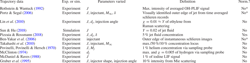
where $A$, $B$ and $C$ are fitting parameters, $d_j$ is the jet diameter and $x$ and $y$ are the streamwise and wall-normal coordinates, respectively. On a purely empirical basis, McDaniel & Raves (Reference McDaniel and Raves1988) proposed a logarithmic scaling of the form $y/d_j = A J \ln [B(x/d_j + C)]$. Both the power law and the logarithmic scaling are used on a regular basis in JISCF research. In table 1, a number of examples are shown for JISCF trajectories fitted to the power-law form. As evident from the examples, trajectories have been reported in the literature as a function of different independent parameters and a range of different trajectory definitions.

Table 1.

Sample of studies reporting JISCF trajectories.

Despite the trajectory laws being applied to a wide range of flow conditions, they do not consider any physical differences between incompressible and compressible flow fields explicitly. The result of this approach is significant scatter in the mean jet trajectories reported between different studies and test conditions, especially in the near field of the jet. This is also evident in the large range of values for the fit coefficients in table 1. As the jet velocity and pressure equilibrate with the cross-flow, turbulent mixing further downstream of the injection point will eventually reach an asymptotic state. Since this asymptotic state is considered to be largely independent of the initial conditions, it is of interest to understand the near field of the jet better. Portz & Segal (Reference Portz and Segal2006) attempted to address the large scatter of mean jet trajectory data in JISCF through a large literature review and a modified, empirical power law that includes the effects of not only the momentum flux ratio, $J$, but also of the boundary layer thickness, $\delta$, the free-stream Mach number, $M_\infty$, and the jet to free-stream molecular weight ratio, $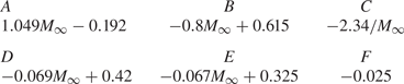MW_j/MW_\infty$. While they report an improved collapse of jet trajectories, all of their parameters are curve fitted as power laws and multiplied to a trajectory law similar to (1.5). The constants in the resulting trajectory equation (1.7) are also empirical functions of the free-stream Mach number (see table 2), making generalization difficult. Importantly, they introduce the concept of an effective momentum flux ratio computed after a normal shock for the given cross-flow Mach number ($M$), see (1.6). As the jet is preceded by a bow shock, this effective $J$ is more representative of the flow conditions that the jet first encounters upon injection than a global, pre-shock $J$. In the equation, $\gamma$ is the specific heat ratio, $p$ is the static pressure, an asterisk denotes sonic conditions and subscripts $1$ and $2$ denote quantities computed before and after a normal shock, respectively,

(1.6)

\begin{gather} J_{2} = J_1 \frac{( \gamma p M^2 )_{\infty,1}}{( \gamma p M^2 )_{\infty,2}} = \frac{( \gamma + 1 )_{\infty,1} \rho^{*}_j U^{*2}_j}{( p \gamma [(\gamma - 1) M^2 + 2] )_{\infty,1}}, \end{gather}

(1.7)

\begin{gather}\frac{y}{d_j} = A (J)^{B} \left(\frac{x}{d_j} +C \right)^{D} \left( \frac{\delta}{d_j} \right)^{E} \left(\frac{MW_j}{MW_\infty} \right)^{F}. \end{gather}

Table 2.

Coefficients for (1.7).

Another relevant result has been reported by Pizzaia & Rossmann (Reference Pizzaia and Rossmann2018). They use the empirical observation by Papamoschou & Hubbard (Reference Papamoschou and Hubbard1993) that the characteristic penetration, $h_{c}$, of a JISCF seems to scale with the momentum flux ratio according to $h_c \propto J^{1/3}$, thereby achieving a reasonable collapse of their trajectory data for a given boundary layer thickness to jet diameter ratio $\delta /d_j$. They report a clear penetration enhancement and stronger turbulent mixing with increasing boundary layer thickness. It appears that for larger $\delta /d_j$ the boundary layer vorticity couples more effectively to the vortical structures of the jet. However, a unified physics-based description of a scaling parameter controlling the JISCF mean trajectory is still missing.

We consider the following questions motivated by the outlined shortcomings: How does turbulent mixing change as a function of momentum flux ratio and injectant properties? What flow physics predominantly control the evolution of the mean JISCF trajectory for underexpanded jets? Can we derive a scaling expression accounting for these dominant flow parameters? To address these questions, we analyse mean and fluctuating jet fluid signal results as a function of jet $MW$, $\gamma$ and $J$. We then consider the controlling factors of the mean JISCF flow field and develop a semi-empirical model for a physics-based JISCF scaling. We validate our approach with trajectory data obtained from our own experimental set-up and from other published studies, extending the parameter space covered. The scaling is used to further discuss the impact of injectant properties on jet trajectories and turbulent mixing.

2. Experimental set-up and methodology

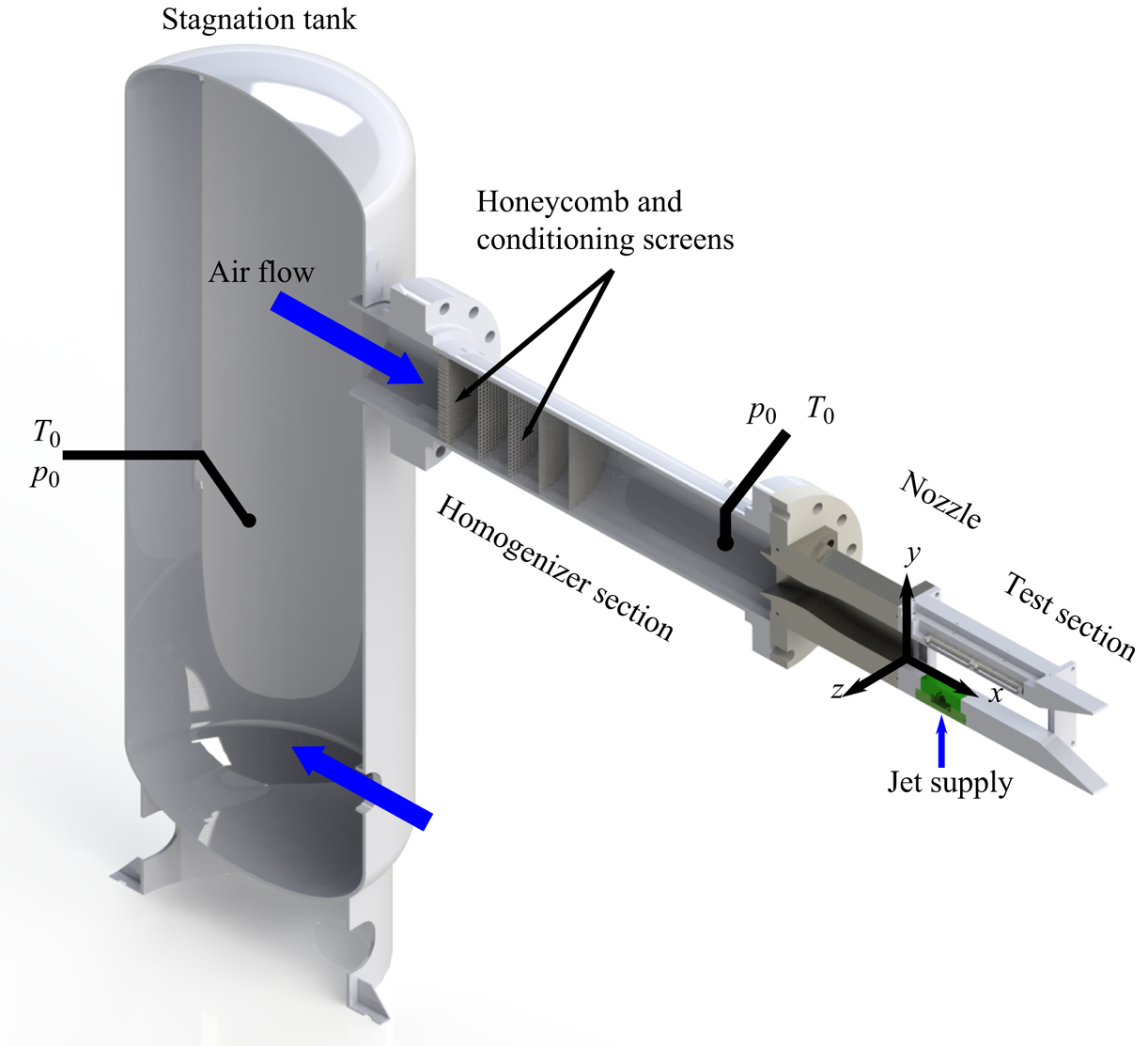
The experimental set-up is situated in one of the high-pressure cells at the Georgia Tech Ben T. Zinn Combustion Lab. Air is supplied by the laboratory's high-pressure system. The system is fed by a Norwalk Compressor and multiple 17 237 kPa storage tanks. The air is filtered and dried in an Ultra Filter refrigerating dryer, before being pumped up to storage pressure. An isometric schematic of the blow-down wind tunnel is shown in figure 2. For the data presented here, the upstream stagnation tank is held at conditions that result in a stagnation pressure of $p_{0,\infty } = 379 \pm 4$ kPa and stagnation temperatures of $T_{0,\infty } = 595 \pm 10$ K, at the end of the homogenizer section. The given ranges correspond to 95 % confidence levels for run-to-run variations. During data acquisition, the tunnel conditions do not change more than 2 %.

Figure 2.

Schematic of the experimental facility used to obtain the presented measurements. The green block in the test section is the injector.

Upstream of the homogenizer, the flow is conditioned by a series of stainless steel honeycomb and wire screens. The converging–diverging nozzle following the homogenizer section has been designed as a minimum length nozzle, using the method of characteristics, for a cross-flow Mach number of 1.7 and an exit cross-section of $8\ \text {cm}\times 8\ \text {cm}$. The $30.5\ \text {cm}\times 8\ \text {cm}$ test section windows provide access for optical diagnostics. The top of the test section provides spaces for static pressure measurements and optical access for lasers and cameras. The bottom section has a $10.15\ \text {cm}\times 6.1\ \text {cm}$ cutout in which injector blocks can be inserted.

Static wall pressure (measured with a Scanivalve DSA 3217 16-channel pressure scanner), particle image velocimetry (PIV) and schlieren measurements are consistent and indicate a Mach number of 1.71 at the jet injection point. See the supplementary material available at https://doi.org/10.1017/jfm.2020.1065 for PIV and schlieren results. Thus, the cross-flow has a static pressure of $p_\infty = 75.8 \pm 1$ kPa and a static temperature of $T_\infty \sim 375 \pm 6$ K. There are some weak shock waves remaining in the test section after the nozzle. They are characterized in more detail in § 2.1 and do not significantly influence our results. Isentropic calculations give a cross-flow reference velocity of $\bar {U}_0 = 664 \pm 6$ m s$^{-1}$, consistent with PIV measurements. The PIV results also indicate a cross-flow turbulence level of $\sigma _{\bar {U}} = 21.4$ m s$^{-1}$, i.e. $\sim$3 %. At the jet injection point the boundary layer thickness is $\delta _{95\,\%} = 5.26$ mm.

The jet injector is designed to provide a well-defined top-hat velocity profile. The jet orifice lies on the test section centreline and has a diameter of $d_j = 2$ mm, which, for a sonic jet, is also the throat diameter. The throat is preceded by a contraction defined through a fifth-order polynomial. The jet injector base acts as a quasi-reservoir in which the supply pressure and temperature of the jet are measured. The injectant gas supply comes from a manifold of four pressurized gas bottles. The injectant pressure is controlled manually with a Tescom 44–1300 series regulator. For all injected gases and pressures, the discharge coefficient is between 0.9 and 0.97. The discharge coefficient was determined by comparing measurements from a MicroMotion Coriolis flow meter with choked nozzle mass flow calculations.

The nominal momentum flux ratios are 1, 2, 4 and 6 for all gases in this study, with jet stagnation pressures in the range of 414–2758 kPa. The jet manifold is heated to keep the injectant stagnation temperature at $T_{j,0} = 309 \pm 10$ K in all cases. During data acquisition, $J$ has a standard deviation of 0.08. Run to run, the desired set point for $J$ can be attained with a standard deviation in the range $\sigma _J = 0.05\text {--}0.23$ (with larger absolute deviation for higher $J$). This range corresponds to a relative run-to-run variation of $\sigma _J/J \approx 3\text {--}5\,\%$. The actually measured momentum flux ratios, from our experiments, are given in table 5. 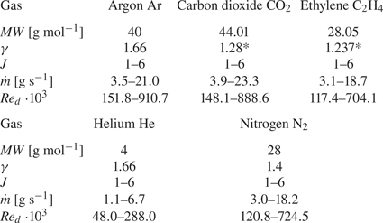During data processing, the measured $J$ values are used and not the idealized, targeted values. The gases used in this study and their main properties of interest are shown in table 3. Systematic variation of the specific heat ratio, $\gamma$, and the molecular weight, $MW$, allows us to identify effects, if any, of these properties on turbulent mixing and the jet mean trajectory evolution.

Table 3.

Properties of gases used for injection and design ranges of nominal mass flow rates and jet Reynolds numbers, $Re_d = \frac{U_j d_j}{\nu_j} $ at the orifice. Entries marked with * depend strongly on temperature, the values reported here are representative at room temperature.

2.1. Cross-flow and boundary layer characterization

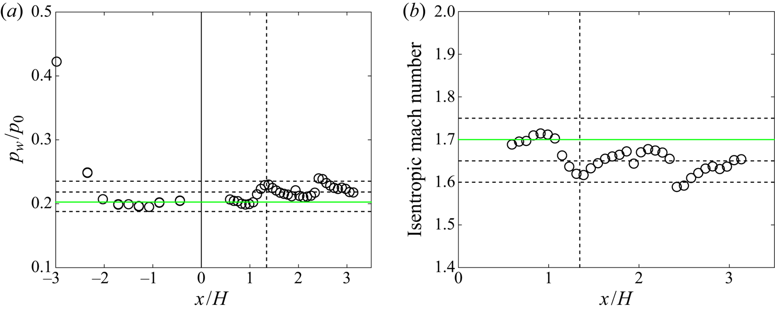
The static wall pressure measurements in figure 3(a) reveal several weak shocks remaining in the test section flow. In the worst case, these correspond to oblique shocks generated by a turning angle of ${\sim }2.7^\circ$, with the Mach number changing from 1.71 to 1.62 and the pressure, density, and temperature increasing by 14.4 %, 11 % and 4 % compared to the pre-shock static values, respectively. The pressure increase of 14.4 % is consistent with wall static pressure measurements. For this kind of oblique shock, the stagnation pressure loss across a wave is ${<}0.1\,\%$, i.e. an approximately constant stagnation pressure should be given along the test section, even after multiple wave crossings. This has been confirmed by Pitot probe measurements, showing that the stagnation pressure in the test section is within 3 % of the measurement upstream, in the homogenizer section. This percentage change is smaller than the total uncertainty of the pressure transducers used.

Figure 3.

Wall pressure measurements and Mach number distribution. The $x$-axis is normalized by the test section height, $H=8$ cm, and measured from the beginning of the test section. The green solid line is the nozzle design condition/Mach number. The dashed vertical line is the location of the injector on the bottom of the test section. The other dashed horizontal lines represent pressures and Mach numbers at ${\rm \Delta} M = 0.05$ intervals. (a) Static wall pressure normalized by the stagnation pressure. In the nozzle the pressures are measured on the side wall, in the test section they are measured on the top wall. (b) Mach number distribution computed via isentropic expansion relations.

Nonetheless, the remaining shock waves cause a change in flow properties across the test section, see figure 3(b) for the change in Mach number. PIV and schlieren measurements in the supplementary material show that the shock wave closest to the jet orifice impinges on the wall $\sim$27 mm behind the injection point. Thus, if there is any direct influence on the jet, it would manifest itself in its downstream wake outside of this study's region of interest. Moreover, the cross-flow velocity is fairly constant, within 3 % of the reference velocity, $U_0 = 664$ m s$^{-1}$. The measured flow properties are considered in the uncertainty analysis in appendix A. Given this flow characterization, we are confident that the presented results are reliable and the flow field changes induced by the remaining waves are not significantly influencing our results.

The boundary layer profile at the jet injection point is shown in figure 4(a). We compare our results with the measurements made by Pizzaia & Rossmann (Reference Pizzaia and Rossmann2018) and the analytical log law after applying the van Driest transformation (White & Corfield Reference White and Corfield2006). We also attempt to curve fit our data to the generalized outer-region turbulent equilibrium boundary layer profile defined by Chauhan, Monkewitz & Nagib (Reference Chauhan, Monkewitz and Nagib2009). Additionally, the development of the 95 % boundary layer thickness is shown in figure 4(b). While the structure of our velocity data roughly resembles a turbulent boundary layer, it does deviate from the utilized references. This is probably due to the pressure gradients induced by the remaining weak shock waves in the test section. The velocities in the near-wall region are lower than predicted by theory, which would correspond to an adverse pressure gradient caused by a compression wave impinging on the boundary layer downstream. That this impingement indeed occurs was discussed earlier in § 2.1.

Figure 4.

(a) Comparison of our supersonic boundary layer profile, after applying the van Driest transformation, to theory and experimental results by Pizzaia & Rossmann (Reference Pizzaia and Rossmann2018). The presented velocity profile is extracted at the jet centreline location. Velocity uncertainty is below 3 % at a 95 % confidence level for the entire boundary layer profile. (b) Streamwise development of the 95 % boundary layer thickness. Also shown is the expected turbulent boundary layer growth assuming a $1/7$ power-law velocity profile (White & Corfield Reference White and Corfield2006). Shaded areas indicate the uncertainty of the boundary layer thickness. The dashed vertical line denotes the location of the jet orifice.

With a cross-flow Reynolds number of $2.31 \cdot 10^{6}$ at the jet orifice (measured from the nozzle exit), it is likely that our experiments are indeed conducted with a turbulent boundary layer. However, it is not a well-defined turbulent boundary layer in the classical sense, i.e. it is a non-equilibrium boundary layer subject to local pressure gradients. The best fit parameters using the boundary layer equation given by Chauhan et al. (Reference Chauhan, Monkewitz and Nagib2009) are the friction velocity $u_\tau = 24.84$ m s$^{-1}$, the wake parameter $\varPi = -0.129$ and the fit boundary layer thickness $\delta = 17.248$ mm.

2.2. Jet fluid signal and trajectory measurements from Mie scattering

Visualization of the jet fluid is achieved using Mie scattering off of Aerosil R974 $\mathrm {SiO_2}$ particles, with the diagnostic set-up shown schematically in figure 5. A 532 nm Big Sky laser is used for particle illumination with a pulse length of 8 ns and 30 mJ pulse$^{-1}$ of energy. The sheet forming optics yield a ${\sim }51$ mm wide and 0.6 mm thick sheet (as measured by the knife-edge method). An Andor Zyla 5.5 camera is used to record the Mie-scattering signal. To improve the fidelity of the Mie-scattering measurements, a part of the laser sheet is split off the main beam. The beam is split using a quartz-glass plate and directed into a rhodamine dye cell. The fluorescence in the cell is imaged with an additional camera to provide an instantaneous laser profile, for shot-to-shot laser profile corrections. After de-warping the images, they are intensity normalized, Median filtered, background and flatfield corrected, laser sheet profile corrected and cropped as required. Accounting for filtering and binning processes during data processing, this set-up results in an effective resolution of ${\sim }110\ \mathrm {\mu }$m. For each data point presented, at least 900 images are available allowing for the computation of statistical properties. Further characterization of the jet flow itself is reported in the supplementary material.

Figure 5.

Optical set-up for Mie-scattering experiments.

To ensure that our seed particles follow the high-speed flow sufficiently, we evaluate the characteristic relaxation time, $\tau _p$, of the Aerosil R974 $\mathrm {SiO_2}$ particles, following the approach of Ragni et al. (Reference Ragni, Schrijer, Van Oudheusden and Scarano2011). The relaxation time is determined across a well-defined oblique shock as $\tau _p = 1.5\text {--}1.6\ \mathrm {\mu }\ \textrm {s}^{-1}$. To compute the resulting Stokes number, we use a characteristic flow time scale derived from laser Doppler velocimetry data in Santiago & Dutton (Reference Santiago and Dutton1997). Their paper reports a maximum root-mean-square (r.m.s.) fluctuating velocity component of $u_{rms} = 178$ m s$^{-1}$. Together with a jet diameter of 2 mm, the relevant large scale time is estimated as $\tau _F = d_j/u_{rms} = 11.2 \, \mathrm {\mu }\ \textrm {s}^{-1}$, yielding a Stokes number of $St =0.14$. Ideally, $St < 0.1$ but the presented technique should be able to follow large scale motions of the jet fluid reliably.

To interpret the Mie-scattering signal, some additional considerations are required. In an isobaric and isothermal flow, the Mie-scattering signal averaged over a finite area is directly proportional to the jet fluid mixture fraction, $f$, in the flow field. This also assumes that the Mie-scattering recordings are fully corrected for background and laser sheet non-uniformities, multiple scattering of light is negligible and the particle image size is diffraction limited. In this study, due to compressibility effects introduced by the sonic jet and the bow shock in front of the jet, a more general expression is required. This expression relates the recorded Mie-scattering signal, $S$, to not only the jet fluid mixture fraction but also the local density (Sautet & Stepowski Reference Sautet and Stepowski1994),

(2.1)

\begin{equation} S = C E_I \alpha_j \frac{\textrm{d} \sigma}{\textrm{d} \varOmega} \textrm{d}\varOmega \rho f. \end{equation}

Here, $C$ is a calibration constant, $E_I$ is the incident laser energy, $\alpha _j$ is the jet seeding rate and $\varOmega$ is the solid angle. The differential scattering cross-section $\textrm {d}\sigma /\textrm {d}\varOmega$ describes the strength of the scattered signal as a function of incident light wavelength and particle size. Furthermore, (2.1) assumes that the line shape of the scattered light is within the transmission window of any filters and lenses in front of the camera chip. All quantities in (2.1) are averaged over the region imaged onto a camera pixel.

Due to fluid element dilatation, variations in temperature and density are decoupled from the jet fluid concentration. Thus, in regions where such effects are strong, the signal $S$ in (2.1) cannot be unique related to $f$, but only to the product $(\rho \cdot f)$ (Sautet & Stepowski Reference Sautet and Stepowski1994). The latter now also reflecting changes in density that are not associated with changes in local composition. Dilatation effects are especially strong close to the injection point of the jet, where flow expansion and compression occur (e.g. the Mach disk, barrel shocks and jet bow shock). Further away from the injection point and the jet centreline, it is more likely that the scattering signal purely represents the local jet fluid concentration. Nonetheless, without a separate density measurement, no definitive statement can be made regarding this issue, in any region of the flow.

The differential scattering cross-section varies strongly and nonlinearly with particle size, i.e. $\textrm {d}\sigma /\textrm {d}\varOmega = f(r_p^n)$. Where $n$ changes from approximately six, in the Rayleigh scattering regime, to two, in the high-frequency optical limit. This represents a problem, if the distribution of particle sizes is not uniform, e.g. due to agglomeration and manufacturing processes. To account for this effect, a technique proposed by Pernpeintner et al. (Reference Pernpeintner, Lauer, Hirsch and Sattelmayer2011) is utilized. They treat the Mie-scattering image recorded by the camera as a convolution of the actual mixture fraction, $f$, and the seeding density, $\omega$. Here, the latter includes effects due to variable $\alpha _j$ and $\textrm {d}\sigma /\textrm {d}\varOmega$. By solving this ill-posed inverse problem, the seeding density probability density function (PDF), $p_\omega$, and the Mie-scattering signal PDF, $p_S$, can be deconvolved and one can recover the PDF of $(\rho \cdot f)$. While this is still not the pure mixture fraction, it improves the fidelity of the results and simplifies interpretation. The formulation of Pernpeintner et al. (Reference Pernpeintner, Lauer, Hirsch and Sattelmayer2011) is modified to a second-order regularization, as it should yield more physically reliable results, i.e. the Tikhonov matrix is not a constant multiplied to the identity matrix, but rather a finite difference operator yielding the second derivative of $p_S$. To find the ideal value of the Tikhonov regularization parameter, the L-curve method is used, in conjunction with the triangle method to find the L-curve corner (Castellanos, Gómez & Guerra Reference Castellanos, Gómez and Guerra2002). Furthermore, a bin size of $11\times 11$ pixels is chosen, yielding at least 121 000 samples for each $p_S$ across the domain. For $p_\omega$, a slightly larger domain very close to the jet exit is chosen, with a bin size of $50\times 50$ pixels yielding 2.25 million samples for $p_\omega$. This PDF also serves as a reference, as it is known a priori that $f \approx 1$, in this region. The dynamic range of the Mie-scattering recordings is reduced from $2^{12}$ to $2^8$, to limit the number of PDF bins.

Using this deconvolution technique, the dependence of the Mie-scattering signal on the calibration constant and $E_I$ in (2.1) is also removed. Thus, the statistics reported in this study are the normalized average $\overline {\rho f}/\overline {\rho f}_0$ and the normalized root-mean-square (r.m.s.) fluctuations $\sqrt {\overline {(\rho f )'^2}}/\overline {\rho f}_0$ of the density–mixture fraction product. In this study, the normalized product of density and mixture fraction will also be referred to as the (normalized) jet fluid signal. Statistical uncertainties reported for the mean and r.m.s. jet fluid signal are computed as described in appendix A.

To some degree, this technique is equivalent to normalizing each recorded Mie-scattering image by an instantaneous reference signal taken in the potential core close to the jet orifice, see Sautet & Stepowski (Reference Sautet and Stepowski1994). The Tikhonov regularization provides one additional parameter to relate the reference signal to the recorded scattering signal and the true tracer particle concentration. Moreover, the binning yields a more meaningful average Mie-scattering signal per bin.

2.3. Jet trajectory definitions

The jet trajectory is determined using the mean jet fluid signal and applying an iterative curve-fitting technique described by Gevorkyan et al. (Reference Gevorkyan, Shoji, Getsinger, Smith and Karagozian2016). To ensure comparability with previous JISCF studies, we add an additional step after finding the maximum jet fluid signal trajectory and determine a 2 % jet fluid signal iso-contour trajectory. Similar approaches have been employed in the majority of published studies, see table 4 The data processing is shown schematically in figure 6 for one data point.

Figure 6.

Jet trajectory determination exemplified with $\mathrm {N_2}$ $J=6$ data. From (a–c): instantaneous Mie-scattering image (after flatfield correction, median filtering and Gaussian filtering), mean image after the numerical inversion procedure and mean image overlayed with the two relevant trajectories determined via the iterative procedure: the maximum jet fluid signal (blue) and the 2 % jet fluid signal trajectory (green). For the trajectories both the actual data (circles) as well as power-law curve fits (solid lines) are shown.

Table 4.

Brief survey of different jet penetration/trajectory definitions in the literature. ‘Norm?’ refers to whether the concentration profiles are re-normalized by the local maximum concentration value. The asterisk denotes ambiguity in the definition if it is based on qualitative markers or burning regions.

Confusion can arise in existing JISCF literature, regarding the effect of jet fluid properties on the jet trajectory and the associated mixing processes, due to inconsistent definitions. Usually, the jet trajectory is measured is defined as some form of concentration iso-contour. The latter being measured in terms of the signal intensity provided by a diagnostic technique, e.g. Gruber et al. (Reference Gruber, Nejad, Chen and Dutton1997a) consider trajectories based on the mean Mie-scattering signal intensity. Given an iso-contour derived from a certain intensity threshold, they come to the conclusion that faster contraction of the iso-contour is a sign of faster mixing. On the other hand, Ben-Yakar et al. (Reference Ben-Yakar, Mungal and Hanson2006) base their penetration analysis on identifying the upper edge of large scale jet structures in instantaneous schlieren snapshots. Thus, they conclude the faster mixing jet instantaneously penetrates deeper into the cross-flow, creating a larger spatial variance. Statistically, the latter manifests itself in a faster dropping mean concentration value, as one moves along the jet at a fixed distance from the centreline, consistent with Gruber et al. (Reference Gruber, Nejad, Chen and Dutton1997a). Thus, while the wording and definitions are different, the outcome is the same. In neither case is the small scale or molecular mixing quantified, only the large scale entrainment rate and turbulent mixing. The results of both studies suggest that the higher $MW$ gas jets mix faster with the cross-flow than the lower $MW$ gas jets, even though the term ‘jet penetration’ is used differently. That higher $MW$ gas jets mix faster has since been supported by a number of other studies (Takahashi et al. Reference Takahashi, Masuya and Hirota2010; Watanabe et al. Reference Watanabe, Kouchi, Takita and Masuya2012).

Further differences in interpretation can arise if concentration profiles are normalized to the local maximum concentration value, i.e. the maximum concentration at a given jet cross-section. Whether ensemble averaged concentration profiles are normalized in this fashion or not varies across literature. A brief survey of studies in table 4 shows that the majority of results is not reported with a normalization to local maximum values. Out of the selected studies, only Pizzaia & Rossmann (Reference Pizzaia and Rossmann2018) normalize their results and base further evaluation on the normalized data. However, some trajectory definitions are ambiguous, e.g. it is not entirely clear how a trajectory based on the maximum signal from OH radicals in reacting jets or schlieren edges in non-reacting jets compare to trajectories based on ensemble averaged normalized and non-normalized concentration iso-contours. In the following, a simple mixing model to explain why normalized and non-normalized concentration profiles can lead to different conclusions, regarding the effect of injectant properties on mixing and entrainment. The model roughly corresponds to turbulent scalar dispersion from a point source governed by a Gaussian process (Pope Reference Pope2000). This description is also applicable to the mixing of incompressible jets in quiescent environments (Bertagni et al. Reference Bertagni, Marro, Salizzoni and Camporeale2019). With this model, the two-dimensional shape of a cross-sectional slice through the concentration field, $C(x,y)$ can be described as,

(2.2)

\begin{equation} C(x,y) = \frac{2 C_0}{\sqrt{\rm \pi} \sigma(x) ( \textrm{erf}(y_{lim}) - \textrm{erf}(-y_{lim}))} \, \textrm{e}^{-{y^2}/{\sigma(x)^2}}. \end{equation}

For the sake of this argument, imagine $x$ to be the coordinate along the jet centreline and $y$ as the transverse coordinate. In the above equation, the spread of the concentration profile is characterized by $\sigma (x)$ and $y_{lim} = 2.576$ is chosen to cover 99 % of the area under a bell curve. $C_0$ is chosen such that at $x=0$, $C(0,0) = 1$ and a linear relationship for the growth of the profile spread is assumed, $\sigma = ax + b$. The rate of growth, $a$ is important in the results while the functional form is not. The trends presented do not change for a polynomial, exponential or power law describing $\sigma (x)$.

Two pseudo-concentration iso-contours are extracted from the resulting $C(x,y)$ profiles. In one case, a global iso-contour threshold is selected as 5 %; in the other case the same threshold is selected, but the profiles are re-normalized with the local centreline ($y=0$) concentration value. The result for the first case is shown in figure 7(a). What is immediately evident is the non-monotonic growth of the iso-contour $y$-coordinate. The contour grows initially and, after a certain distance, starts contracting again, eventually converging back to the centreline. This is due to the fact that for fast enough mixing the threshold concentration value is eventually equivalent to the maximum centreline concentration value. Away from the centreline the scalar concentration has been diluted below the threshold value. In fact, even the centreline concentration will be below the threshold for further mixing, but it is the closest that local conditions can still get to it. In this scenario, the peak $y$-coordinate depends on the rate of growth of $\sigma$. This is equivalent to saying that it depends on how fast the fluids are mixing. For a slow enough mixing process, $y$ could keep growing beyond the limits of the current example and no contraction towards the centreline would be observable. For a faster process, the peak $y$-coordinate is larger and reached faster. In the second case, figure 7(b), no matter the growth rate of $\sigma$, the $y$-coordinate of the iso-contour will keep increasing. However, the rate at which it increases does depend on the growth rate of $\sigma$. Thus, in this case, faster mixing yields a faster, monotonically growing $y$-coordinate.

Figure 7.

Examples of the two different approaches with which concentration iso-contour based jet penetrations (or jet trajectories) are determined in JISCF literature. The threshold here is $C = 0.05$. The black concentration profiles are plotted proportional to the $x$-coordinate and only for the lower $\sigma$ growth rate of $a = 0.2$. (a) Concentration iso-contours of a Gaussian mixing process. The growth rate $a$ of the profile spread $\sigma$ controls when the $y$-coordinate starts reducing again after the initial growth. (b) Concentration iso-contours of a Gaussian mixing process for which the profiles at each $x$-coordinate have been normalized by the centreline concentration. The growth rate $a$ of the profile spread $\sigma$ determines how fast the $y$-coordinate of the iso-contour grows.

Of course a JISCF is not exactly analogous to an incompressible point source. Especially the existence of the counter-rotating vortex pair will cause deviations from an ideal Gaussian process and break the axial symmetry assumed in the model, e.g. see the spanwise measurements of Lin et al. (Reference Lin, Ryan, Carter, Gruber and Raffoul2010). Differences in lateral entrainment and mixing of the jet could also change the trends shown in figure 7.

For example, large enough lateral entrainment could prevent a steady rise of the normalized trajectory and cause it to become parallel to or even to dip towards the line of maximum concentration (which itself will eventually be parallel to the cross-flow). Compressibility effects in the near field of the jet might also play a role. However, even if the JISCF is not correctly described by a Gaussian process, the fact remains that jet penetration or trajectory defined by locally normalized concentration values should always exceed the non-normalized case in its transverse extent. Moreover, the selection of the threshold value also influences the rate at which $y$ changes, so that small differences have to be expected even between studies that are identical save for the selected concentration threshold values, see for example figure 11 in Watanabe et al. (Reference Watanabe, Kouchi, Takita and Masuya2012). To the authors’ best knowledge, if the principles described in this section are applied, studies using different definitions and criteria, largely agree on the effect of injectant properties on mixing and entrainment in JISCF flow fields.

3. Results

We discuss mean and fluctuating r.m.s. jet fluid signal data as well as mean jet trajectories. Planar JISCF jet fluid signal measurements were collected for the injectants and measured momentum flux ratios listed in table 5. The r.m.s. fluctuating part of the jet fluid signal can exhibit some noisiness, i.e. relatively rapid spatial changes of signal values. Given this noisiness and the measurement of $(\rho \cdot f)$, not purely $f$, only qualitative trends and relative changes in the jet fluid signal measurements are considered in the following discussions.

Table 5.

Targeted $J$ values and measured $J$ values for each gas used in the presented study.

3.1. Mean and fluctuating jet fluid signals

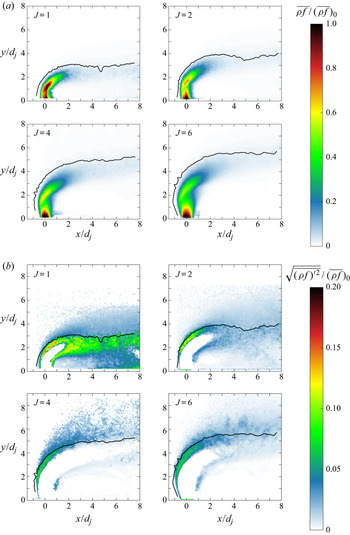
Argon jet results are presented in figure 8. The coordinates are normalized with the jet diameter, $d_j = 2~mm$. Black solid lines represent the jet trajectory, defined as the windward 0.02 jet fluid signal iso-contour. In some cases, the jet fluid signal near the wall is clipped to exclude reflections from further evaluation. The mean jet fluid signal, see figure 8(a), is decreasing downstream of the injection point, as the injectant is entrained into the cross-flow. The non-monotonic behaviour around $y/h_c = 1\text {--}2$, with $\rho f$ suddenly increasing again over a short distance, is due to density effects, i.e. the barrel and Mach disk shock formed by the jet. While there are small differences due to gas properties and turbulent mixing, this general jet expansion and compression behaviour can be observed in all cases. We also observe that, in all cases, the jet penetration appears to increase with increasing $J$, as would be expected. The argon mean jet trajectories at $J=1$ and $J=2$ penetrate deeper into the cross-flow as $x/d_j$ increases. Around $x/d_j = 5$, the trajectories dip down slightly and then continue to move upwards into the cross-flow. One could associate this dip with the presence of an expansion region behind the bow shock. However, the dip is not as pronounced for the $J=4$ and $J=6$ cases, where the jet penetration seems to reach more of a plateau around $x/d_j = 3$. Thus, it appears more likely that the dipping behaviour is a result of turbulent mixing and the definition used for the jet trajectories, instead of just the expansion fan behind the bow shock. A more in-depth discussion of the reasons for the dip, based on turbulent mixing and the trajectory definition, was given in § 2.3. This preceding discussion also suggests that, even at higher $J$, the dip should occur eventually, possibly outside the current field of view. That, at higher $J$, the dips are not visible here is either due to the availability of more jet fluid, i.e. higher jet mass flow rates, or changes in the interaction between jet and boundary layer.

Figure 8.

Jet fluid signal results for argon. The nominal momentum flux ratio is indicated in the upper left corner. The black solid line is the corresponding 2 % jet trajectory. (a) Mean mixture fraction for argon. (b) The r.m.s. jet fluid signal for argon.

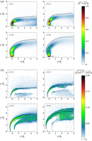
Differences in the mean trajectory development are evident, when comparing the argon to the ethylene results in figure 9(a). As opposed to the argon trajectories, the ethylene trajectories exhibit a dip around $x/d_j = 5$ at all momentum flux ratios considered. According to the discussions in § 2.3, this could suggest a difference in turbulent mixing processes between argon and ethylene injection.

Figure 9.

Jet fluid signal results for ethylene. The nominal momentum flux ratio is indicated in the upper left corner. The black solid line is the corresponding 2 % jet trajectory. The $J=6$ case had to be processed with a stronger Gaussian filter, than the other cases, to achieve convergence in the solution of the inverse problem yielding the jet fluid signal field. (a) Mean mixture fraction for ethylene. (b) The r.m.s. jet fluid signal for ethylene.

The carbon dioxide trajectories in figure 10(a) also show a dip at all $J$. However, at $J=6$ the dip occurs already at $x/d_j = 3\text {--}4$. Thus, indicating faster turbulent mixing processes at $J=6$ than in the argon and ethylene cases. The increase in turbulent mixing is probably due to the lower specific heat ratio of the carbon dioxide jet, see table 3, as the molecular weights are almost equal. The difference in $\gamma$ causes a difference in the sonic velocity upon injection, i.e. it is approximately 10 % lower for carbon dioxide, with the speed of sound given by $a=\sqrt {\gamma (\mathcal {R}/MW) T}$. Experimental evidence suggests that, for JISCF, the initial convective velocities and Mach numbers in the jet shear layer are proportional to the jet velocities (Gruber et al. Reference Gruber, Nejad, Chen and Dutton1997b; Ben-Yakar et al. Reference Ben-Yakar, Mungal and Hanson2006). Thus, the argon jet is likely to result in higher convective velocities and Mach numbers than the carbon dioxide jet (see (1.2) and (1.3)), suppressing hydrodynamic instability growth and turbulent mixing.

Figure 10.

Jet fluid signal results for carbon dioxide. The nominal momentum flux ratio is indicated in the upper left corner. The black solid line is the corresponding 2 % jet trajectory. (a) Mean mixture fraction for carbon dioxide. (b) The r.m.s. jet fluid signal for carbon dioxide.

In contrast to the three gases discussed so far, the helium jet trajectories in figure 11(a) do not show any dip within the present field of view. Moreover, at the downstream edge of the images, the helium jet trajectories penetrate deeper into the cross-flow than the other gas trajectories examined so far. Especially at $J=6$, helium exceeds $y/d_j = 6$, while argon, ethylene and carbon dioxide jets do not reach that deep into the cross-flow. Finally, the extent of the high intensity jet core region appears longer for helium than for the other gases. This suggests slower turbulent mixing processes in the case of helium injection, at all momentum flux ratios. In agreement with the results by Gruber et al. (Reference Gruber, Nejad, Chen and Dutton1997a) and Ben-Yakar et al. (Reference Ben-Yakar, Mungal and Hanson2006), the slower turbulent mixing is due to the much lower molecular weight of helium compared to argon, ethylene and carbon dioxide, (see table 3 for comparison). Consequently, helium has a $\geq 2.5$ times higher sonic velocity upon injection than the other gases, resulting in the largest convective velocities and Mach numbers and suppressing turbulent mixing the most. The specific heat ratio also plays a role, but the relative differences for this property are much smaller.

Figure 11.

Jet fluid signal results for helium. The nominal momentum flux ratio is indicated in the upper left corner. The black solid line is the corresponding 2 % jet trajectory. (a) Mean mixture fraction for helium. (b) The r.m.s. jet fluid signal for helium.

Finally, the mean jet fluid signal results for the nitrogen jets are shown in figure 12(a). Although the molecular weight of nitrogen is essentially the same as that of ethylene, the nitrogen mean trajectories only exhibit a dip at $J=1$. Moreover, the mean jet penetration at the downstream edge is more comparable to the helium results and at $J=2\text {--}6$ even exceeds the measured helium mean penetration into the cross-flow. The differences between the nitrogen and ethylene results can potentially be explained by differences in the specific heat ratio. That is, the lower specific heat ratio of ethylene ($\gamma = 1.237$) leads to faster turbulent mixing than for nitrogen ($\gamma = 1.4$). However, the comparable penetration depths of nitrogen and helium jets require further analysis by considering the mean jet trajectories themselves in more detail in § 3.2.

Figure 12.

Jet fluid signal results for nitrogen. The nominal momentum flux ratio is indicated in the upper left corner. The black solid line is the corresponding 2 % jet trajectory. (a) Mean mixture fraction for nitrogen. (b) The r.m.s. jet fluid signal for nitrogen.

Before moving on to the mean jet trajectories, we discuss the fluctuating r.m.s. jet fluid signal in more detail. For argon, in figure 8(b), the intensity and extent of jet fluid signal fluctuations can be seen to change with increasing $J$. This is likely a consequence of the jets changing expansion, changing interaction with the cross-flow boundary layer and changing interaction with the cross-flow itself. At $J=1$, regions with elevated jet fluid signal fluctuations occur over larger parts of the flow field. The length of the jet potential core appears to peak at $J=4$. For the ethylene jet in figure 9(b), the differences between momentum flux ratios, with regard to signal fluctuation and intensity, is smaller than for the argon cases. With increasing momentum flux ratio, the jet fluid signal fluctuations appear slightly more distributed in the plane of symmetry. The influence of a stronger Gaussian filter, used to converge the $J=6$ inversion, is discernible in the slightly more smeared appearance of the results. The jet potential core seems to increase in size up to $J=4$. At $J=1$ and $J=2$, the potential core is more pronounced than in the argon case, while at $J=4$ and $J=6$ the potential core is shorter and less clearly delineated. With carbon dioxide injection (see figure 10)(b), the trends are comparable to the argon results. At $J=6$, there is a change in the appearance of the potential core, with a small region of increased fluctuations close to the location of the jet barrel shock around $x/d_j \approx 0.5$, $y/d_j \approx 3$. The helium jet fluid signal fluctuations in figure 11(b) are distinctly different from the other gases discussed so far. The spatial extent of elevated fluctuation values increases with the momentum flux ratio. Simultaneously, the length of the potential core is decreasing with $J$. The ubiquitous elevated fluctuations at $J=4$ and $J=6$ suggest the existence of larger amounts of unmixed jet fluid than in the other injectant cases. The nitrogen jet fluid signal fluctuations in figure 12(b) are comparable to the ethylene jet results (similar molecular weight), especially at $J=1$ and $J=2$. However, at higher momentum flux ratios, regions of elevated fluctuating signals are more distributed, suggesting slower turbulent mixing than for the corresponding ethylene cases.

Certain trends as a function of jet injectant properties and momentum flux ratio can be identified. At high molecular weight and high specific heat ratio (e.g. argon), as the momentum flux ratio increases, elevated jet fluid signal fluctuations are increasingly localized at the edge of the windward jet shear layer, close to the identified 2 % jet trajectory. As the molecular weight decreases, this trend reverses, i.e. for helium, the fluctuations are highly localized at $J=1$ and much more distributed at $J=6$. The same trend can be observed for ethylene and nitrogen to a lesser degree. Moreover, the peak fluctuations are more likely to occur outside the trajectory contour as molecular weight decreases. This trend suggests that, for such cases, large scale turbulent mixing structures do not penetrate as deeply into the jet, decreasing turbulent mixing efficiency. An observation which has also been made by Gruber et al. (Reference Gruber, Nejad, Chen and Dutton1997a). Decreasing the specific heat ratio also changes the turbulent mixing processes, but the differences are more subtle, due to the smaller relative changes investigated. Nonetheless, comparing argon to carbon dioxide, and nitrogen to ethylene results, suggests slightly more distributed jet fluid signal fluctuations as $\gamma$ decreases. To summarize, trends in the jet fluid signal fluctuations suggest that the interaction between jet, cross-flow and cross-flow boundary layer changes with both the momentum flux ratio and molecular weight. Furthermore, a switch in trends is observed as the molecular weight changes.

At higher investigated values of $J$, the observed behaviour is consistent with the convective Mach number concept and the observations made by Gruber et al. (Reference Gruber, Nejad, Chen and Dutton1997a) for helium and air jets and Ben-Yakar et al. (Reference Ben-Yakar, Mungal and Hanson2006) for hydrogen and ethylene jets. The lighter gases exhibit stronger remaining mixture fraction fluctuations downstream of injection, suggesting that entrainment and mixing are less effective than for the heavier gases. However, especially at $J=1$, this trend is not as clear and heavier gases show stronger remaining fluctuations downstream of the injection point. In the following, a speculative explanation for these observations is proposed, based on the convective Mach number model (Papamoschou & Roshko Reference Papamoschou and Roshko1988).

At $J=1$ the jet interacts more with the boundary layer region. Due to the smaller velocities of high $MW$ gas jets (e.g. argon and carbon dioxide) and the low-speed boundary layer, instabilities can form and effectively entrain cross-flow fluids. In the case of the lower $MW$ gas jets (e.g. helium), the jet velocities are much larger and the formation of instabilities and turbulent mixing structures is suppressed to some degree. Thus, the higher $MW$ gases would initially experience stronger turbulent mixing, i.e. stronger and more distributed jet fluid signal fluctuations. At the same time, the lower $MW$ gas jets would experience weaker perturbations with suppressed growth. Since the velocity difference between jet and cross-flow only decreases with downstream distance, the shear mechanisms initiating hydrodynamic instability also become weaker, slowing down turbulent mixing further. At $J = 2$, an intermediate regime for the specific experimental set-up in this study is achieved. Interacting more with the high flow speeds outside the boundary layer, the higher $MW$ injectants are subjected to increasing instability suppressing effects, but also increasing turbulent mixing rates due to the higher momentum flux ratio. However, that turbulent mixing rates increase with $J$ has so far only been shown explicitly for incompressible jet in crossflow (JICF) (Hasselbrink & Mungal Reference Hasselbrink and Mungal2001). At $J=4$, we have to assume that, while mixing rates are increasing for all gases, the suppression of instabilities on the jet interface increases faster for the low $MW$ gases than the high $MW$ gases. If the assumption holds true, then the turbulent mixing of the high $MW$ gases progresses faster, causing peak fluctuating values to drop off earlier. The lower $MW$ gases continue to exhibit elevated fluctuations further downstream, as the turbulent mixing process is still ongoing. For this particular condition, nitrogen behaves qualitatively similar to helium, which is probably due to its $MW$ being lower than that of argon and carbon dioxide, but its $\gamma$ being higher than that of ethylene. Ethylene, at $J=4$, being qualitatively more similar to the higher $MW$ gases, argon and carbon dioxide. Finally, $J=6$ is a continuation of the trends at $J=4$. The higher $MW$ gases are now subject to stronger instability suppressing effects. Meanwhile, the lower $MW$ gases, specifically helium, continue to show high and distributed jet fluid signal fluctuations, indicative of high convective Mach numbers and incomplete turbulent mixing.

The assumption, that suppression of hydrodynamic instabilities increases faster with $J$ for lower $MW$ gases, is tested via an analytic point estimate of the jet velocity, similar to the point estimate of $M_c$ made by Gruber et al. (Reference Gruber, Nejad, Chen and Dutton1997a). Due to the lack of velocity data in this study, $M_c$ cannot be estimated directly. Instead, the peak jet velocity magnitude just before the Mach disk, or barrel shock, is calculated. For this velocity to be meaningful, the convective velocity (or convective Mach number) has to increase with it. Since the convective velocity depends on the (wall-normal) jet velocity, this is likely to be true. The velocity magnitude just before the Mach disk is calculated as,

(3.1)

\begin{equation} U_{j,1} = M_{j,1} \sqrt{\gamma_j R_j T_{0,j} \left( 1 + \frac{\gamma_j - 1}{2} M_{j,1}^2 \right)^{-1}}. \end{equation}

The Mach number just before the Mach disk of the jet, $M_{j,1}$, is calculated by combining an isentropic expansion relation for pressure with a normal shock relation across the Mach disk,

(3.2)

\begin{equation} \frac{p_{j,2}}{p_\infty} = \left(\frac{2 \gamma_j M_{j,1}^2 - (\gamma_j - 1)}{\gamma_j + 1} \right) \cdot \frac{( 1 + \frac{1}{2} ( \gamma_\infty - 1) M_\infty^2 )^{{\gamma_\infty}/({\gamma_\infty - 1})}}{( 1 + \frac{1}{2} ( \gamma_j - 1) M_{j,1}^2 )^{{\gamma_j}/({\gamma_j - 1})}} \frac{p_{0,j}}{p_{0,\infty}}. \end{equation}

This equation is the same as used by Gruber et al. (Reference Gruber, Nejad, Chen and Dutton1997a) and can only be solved for $M_{j,1}$ if the pressure ratio $p_{j,2}/p_\infty$ is known. Gruber et al. (Reference Gruber, Nejad, Chen and Dutton1997a) use $p_{j,2}/p_\infty = 3.1$. There is no reason to expect $p_{j,2}/p_\infty$ to be constant for different experimental set-ups, cross-flow Mach numbers and momentum flux ratios. However, Gruber et al. (Reference Gruber, Nejad, Chen and Dutton1997a) also showed that changing $p_{j,2}/p_\infty$ only moderately affects the value of $M_{j,1}$. Thus, the constant value of 3.1 is used in our study as well, keeping in mind that it can introduce an uncertainty of up to $M_{j,1} \pm 1$.

Using the approach outlined above, the jet velocity just before the Mach disk is presented in figure 13(a). The strong dependence on the molecular weight of the injectant is evident. Smaller differences due to changes in specific heat ratio can also be discerned. Helium, as expected, has the highest jet velocities and, thus, the overall highest convective Mach number (see also the estimate by Gruber et al. Reference Gruber, Nejad, Chen and Dutton1997a). The differences between the other four gases are smaller than the difference to helium, which makes sense given the relative changes in $MW$. Due to differences in $\gamma$, values of $U_{j,1}$ are consistently higher for carbon dioxide and ethylene than argon and nitrogen, respectively. This contradicts the observation that, for similar $MW$, the lower $\gamma$ gases seem to exhibit faster turbulent mixing. However, at the injection point itself, the (sonic) jet velocities are higher for argon and nitrogen, by a small margin. That is, sonic velocities of ${\sim }280$ m s$^{-1}$ for argon and ${\sim }323$ m s$^{-1}$ for nitrogen compared to ${\sim }253$ m s$^{-1}$ for carbon dioxide and ${\sim }314$ m s$^{-1}$ for ethylene, respectively. This suggests that the idealized isentropic expansion process considered here, by itself, does not capture the development of the turbulent mixing process completely. Velocity differences directly at the injection point might be able to influence turbulent mixing results further downstream, as well.

Figure 13.

Jet velocity estimates upstream of the Mach disk as a function of momentum flux ratio. Darker colours equal higher $MW$. (a) Jet velocity upstream of the Mach disk. (b) Jet velocity derivative with respect to momentum flux ratio.

The change in jet velocity with momentum flux ratio, just before the Mach disk, is plotted in figure 13(b). As assumed for our explanation of trends in the fluctuating jet fluid signal, the jet velocity increases faster with momentum flux ratio for lower $MW$ gases. At lower momentum flux ratios, i.e. $J<4$, the differences are pronounced and of the order of ${\rm \Delta} \partial U_{j,1}/\partial J = 20$ m s$^{-1}$. At higher $J$, the increase in jet velocity is reduced and all gases seem to converge at values below $\partial U_{j,1}/\partial J = 10$ m s$^{-1}$. Interestingly, in figure 13(b), nitrogen lies on top of the carbon dioxide line, due to its higher specific heat ratio. Although the analytical estimate provides some support for the assumption that $M_c$ increases faster with $J$ for lower $MW$ gases, the results are contingent on several simplifying assumptions. For a proper test, the convective velocity, the jet and cross-flow velocities, or the pressure ratio $p_{j,2}/p_\infty$ as a function of $J$ should be measured directly. However, this is outside the scope of this study and left for future work.

The findings presented in this section have implications for engineering designs. They imply that, to achieve optimal turbulent mixing using JISCF, the boundary layer, the jet operating point, and the injectant properties have to be taken into account simultaneously. A high level indicator of turbulent mixing efficiency is the easily estimated sonic velocity upon injection. The higher the sonic velocity, the slower turbulent mixing will be. Moreover, for a given injectant, certain flow conditions might be desirable to optimize turbulent mixing. For example, the presented analysis indicates that, if a low $MW$ gas, such as $\mathrm {H}_2$, is desired as injectant in a supersonic combustor, a low momentum flux ratio and thicker boundary layer can be beneficial to maximize turbulent mixing. Higher $MW$ gases, on the other hand, can profit more of high momentum flux ratios and thinner boundary layers.

3.2. JISCF trajectory considerations

In this section, we develop a semi-empirical, physics informed JISCF trajectory scaling. This new scaling is then validated and compared to existing scalings, using our own data as well as results available in the literature. Finally, we use the scaling to discuss the influence of jet injectant properties further.

3.2.1. Development of a physics informed jet trajectory scaling

To develop a JISCF mean trajectory scaling, the momentum balance technique presented for an incompressible JICF by Muppidi & Mahesh (Reference Muppidi and Mahesh2005), is extended to a high-speed compressible cross-flow. Applying momentum balance analysis to a JISCF and estimating a characteristic scale has been attempted before by Zukoski & Spaid (Reference Zukoski and Spaid1964). However, their approach balances the momentum components parallel to the test section wall and neglects the existence of velocity gradients due to the boundary layer and cross-flow-dependent shock structures. The analysis presented here could be viewed as an extension and generalization, respectively, of these two studies.

For a meaningful extension of the technique by Muppidi & Mahesh (Reference Muppidi and Mahesh2005), similarities and differences between incompressible JICF and JISCF have to be considered. In both cases, a wall boundary layer represents a region with lower momentum flux that allows for an increase in the jet's cross-flow penetration. Additionally, in the case of a JISCF, the interaction of the jet with the supersonic cross-flow leads to the formation of a bow shock in front of the jet. Above the sonic line in the boundary layer, the bow shock will extend the region of reduced momentum flux as incoming cross-flow fluid is shocked to much lower velocities. The change in velocity is especially strong through the almost vertical part of the shock, see figure 1(b) and the instantaneous schlieren visualizations in figure 14. Furthermore, as the sonic underexpanded jet expands into the cross-flow, the jet fluid eventually will be forced to match the ambient pressure through flow features called the barrel shock and the Mach disk, see the mean flow field images in figure 14 for examples. This reduces the momentum flux of the jet itself.

Figure 14.

Schlieren visualization of a $\mathrm {N_2}$ jet in a Mach 1.71 cross-flow. Top row $J = 2$, bottom row $J = 6$. Left column: instantaneous images, middle column: mean images, right column: r.m.s. images. Brighter colour corresponds to higher intensity values. Red lines mark flow field features of interest for the scaling developed here. The variations in the salient flow features with $J$ are clearly visible.

Based on these observations, we can expect that at a characteristic penetration height, $h_c$, the momentum of the jet will be rapidly overwhelmed by the cross-flow momentum. This is corroborated by the topology of the r.m.s. fields in figure 14. The windward edge of the jet shear layer, in the r.m.s. images, can be considered as an indicator of the jet trajectory. At a certain height, this trajectory quickly turns and runs almost parallel to the cross-flow. The specific height at which this occurs should lie in a region where the bow shock becomes weaker and the jet fluid has passed through the jet shock system. Writing the integral momentum balance up to this penetration height behind the bow shock yields,

(3.3)

\begin{equation} d_j \int_0^{h_c} \rho_{cf}(x,y) U_{cf}^2(x,y) \,\textrm{d} y = C_h \int_{A_j} \rho_j(x,z) U_j^2(x,z) \,\mathrm{d}A_j, \end{equation}

where $C_h$ is a constant of proportionality and cross-flow properties (subscript $cf$) are all functions of the position in the flow field due to the boundary layer and the bow shock. The integral on the left-hand side is multiplied by $d_j$, assuming that flow properties are essentially constant over the spanwise width of the jet orifice. The integral on the right-hand side is taken over the jet orifice area and the $y$-dependence is neglected. Because it is postulated that the momentum flux deficits introduced by the flow's compressibility features control the mean jet evolution, an integration up to regions of entirely constant velocity is not necessary. As described by Muppidi & Mahesh (Reference Muppidi and Mahesh2005), the momentum balance in (3.3) assumes that the pressure gradient imposed on the jet by the cross-flow is causing the jet deflection. This pressure gradient is proportional to the cross-flow momentum flux. Furthermore, it assumes that significant jet deflection occurs once the transversely integrated cross-flow momentum flux is comparable to the initial jet momentum flux.

To solve the integral relationship in (3.3), several simplifications have to be made. The velocity profile of choked sonic jets upon injection closely resembles a top-hat velocity profile, i.e. $U_j(x,z) \approx \textrm {const.} = U^*_j$ and $\rho _j = \textrm {const.} = \rho ^*_j$. See the supplementary material available at https://doi.org/10.1017/jfm.2020.1065 for actual measurements of jet velocity profiles in this study. Moreover, as suggested for the incompressible case by Muppidi & Mahesh (Reference Muppidi and Mahesh2005), the cross-flow velocity profile in front of the jet is approximated by a linear function $U_{cf}(x,y) \approx U_{\infty ,2} \cdot y/(\delta +\delta _s)$, where the subscript $2$ denotes properties after a normal shock. Here, $\delta$ is the boundary layer thickness and $\delta _s$ is the extension of the boundary layer effects due to the bow shock momentum flux reduction. Finally, we assume that, for this scaling, $\rho _{cf}(x,y) = \rho _{cf,2}$ is sufficient. This simplifies the relationship in (3.3) to,

(3.4)

\begin{equation} \int_0^{h_c} \left( \frac{y}{\delta+\delta_s} \right)^2\, \mathrm{d} y = \frac{1}{4} C_h {\rm \pi}d_j J_2.\end{equation}

Solving for the characteristic penetration height, $h_c$, yields,

(3.5)

\begin{equation} \frac{h_c}{d_j} = \left[ \frac{3}{4} J_2 {\rm \pi}C_h \left( \frac{\delta + \delta_s}{d_j} \right)^2 \right]^{{1}/{3}}.\end{equation}

While it is expected that JISCF flow features scale with $h_c$, the characteristic penetration does not represent any physical features of the flow. Any direct correspondence between geometrical features of the JISCF flow field and $h_c$ should be regarded as coincidental.

The shock induced momentum flux deficit region, $\delta _s$, is estimated using a combination of blast-wave and oblique shock wave theory. To apply results from blast-wave theory, it is assumed that the JISCF can be viewed as the upper half of a blunt-nosed cylinder. An assumption which has been made successfully before by Zukoski & Spaid (Reference Zukoski and Spaid1964). The approximate radial coordinate, $r$, of a shock wave around such a body can be computed from results available in the literature (Anderson Reference Anderson2006, chap. 4),

(3.6)

\begin{equation} \frac{r}{d_{cyl}} = 0.795 C_D^{{1}/{4}} x^{{1}/{2}},\end{equation}

where $d_{cyl}$ is the diameter of a blunt-nosed cylinder and $C_D$ is the drag coefficient. We assume that the momentum flux deficit region ends once the cross-flow Mach number behind the bow shock is no longer subsonic, i.e. $M_2 = 1.01$. Using planar oblique shock relations, the corresponding bow shock angle, $\beta$, can be found. As $dr/{\textrm {d} x} = \tan \beta$, the $x$-coordinate in (3.6) can be replaced, yielding,

(3.7)

\begin{equation} \frac{r}{d_{cyl}} = 0.316 \frac{C_D^{{1}/{2}}}{\tan\beta}.\end{equation}

The two remaining unknowns are the equivalent body size, $d_{cyl}$, and the drag coefficient. The equivalent body size of the JISCF is replaced with an empirical observation by Papamoschou & Hubbard (Reference Papamoschou and Hubbard1993), i.e. the characteristic ‘size’ of the jet is proportional to the momentum flux ratio to the one-third power, $d_{cyl} \propto J_2^{{1}/{3}} d_j$. With this relationship, (3.7), and introducing an additional proportionality constant $C_r$, we write an explicit expression estimating $\delta _s$ in (3.8).

(3.8)

\begin{equation} \frac{\delta_s}{d_j} \equiv \frac{r}{d_j} = \frac{0.316}{\tan\beta} C_r C_D^{{1}/{2}} J_2^{{1}/{3}}. \end{equation}

The drag coefficient, $C_D$, of a JISCF, as well as two proportionality constants, $C_h$ and $C_r$, remain to be determined. The drag coefficient is set to $C_D = C_{p,max}/2$, where $C_{p,max}$ is the pressure coefficient relative to the stagnation pressure behind a normal shock wave. This is a result of Lee's modified Newtonian law applied to a spherical body (Anderson Reference Anderson2006, chap. 3). The latter being a shape similar to a blunt-nosed cylinder with regard to the drag coefficient. The value of $C_{p,max}$ converges to $C_{p,max} = 2$ in the limit of infinite Mach number and $\gamma _\infty \rightarrow 1$. The constants $C_h$ and $C_r$ are determined by comparing trends of the derived characteristic penetration scale, $h_c$ in (3.5), with the empirical results of Portz & Segal (Reference Portz and Segal2006). The pre-multiplier of their curve fit, see (1.7), is summarized in one expression,

(3.9)

\begin{equation} \frac{h_C^P}{d_j} = A (J_1)^{B+({1}/{2})D} \left( \frac{\delta}{d_j} \right)^{E}. \end{equation}

The dependence on the molecular weight is neglected because it is weak and $h_c$ does not account for it either. The additional $1/2 D$ factor, in the exponent of the pre-shock momentum flux ratio, is due to the particular form assumed for the relevant $x$-direction scaling, i.e. $x/J^{{1}/{2}} d_j$. The $x$-direction scaling is described and justified in more detail later. Values for $h_C^P/d_j$ are computed over the following parameter range: $M_1 = 1.5\text {--}3.5$, $\delta /d_j = 0.1\text {--}10$, $J_1 = 0.1\text {--}30$.

A three-parameter curve fit is performed using nonlinear least squares to fit the developed expression for $h_c$ to the space spanned by $h_C^P$. The result shown in figure 15 is visualized as a projection from the four-dimensional fitting space, with three independent parameters ($J_1$, $\delta /d_j$ and $M_1$), to three dimensions with two independent parameters. The $R^2$ value of the fit is 0.89 with $C_h = 0.084$ and $C_r = 17.236$. The value of $C_h$ is comparable in magnitude to the value measured by Muppidi & Mahesh (Reference Muppidi and Mahesh2005) for incompressible JICF, i.e. 0.05. This could imply that the fundamental interaction between the jet and cross-flow induced pressure gradients does not change from subsonic to supersonic flows.

Figure 15.

Results of curve fitting the expression in (3.5) to the empirical results of Portz & Segal (Reference Portz and Segal2006). Every 41st data point used for the curve fit is shown.

The value of $h_c/d_j$ is used to scale the non-dimensional transverse jet penetration $y/d_j$. However, the correct scaling for the $x$-coordinate is subject to an ongoing debate. In non-reacting incompressible JICF studies, both $x/J d_j$ and $x/J^{{1}/{2}} d_j$ have been discussed. Some theoretical and experimental results suggest $x/J^{{1}/{2}} d_j$ as the more relevant scaling (Broadwell & Breidenthal Reference Broadwell and Breidenthal1984; Smith & Mungal Reference Smith and Mungal1998; Hasselbrink & Mungal Reference Hasselbrink and Mungal2001). However, other studies, such as the one by Gevorkyan et al. (Reference Gevorkyan, Shoji, Getsinger, Smith and Karagozian2016), achieve better trajectory collapse using a $x/J d_j$ scaling, suggesting that jet operating conditions have some influence on the ideal scaling parameter. Recently, in a compressible JISCF study, Pizzaia & Rossmann (Reference Pizzaia and Rossmann2018) had success collapsing their jet trajectories using the $x/J^{{1}/{2}} d_j$ scaling. Thus, this study favours the latter scaling, but will assess potential improvements in trajectory correlations using the $x/J d_j$ scaling, as well.

Based on the preceding analysis, and in the spirit of past JISCF studies, a JISCF trajectory law utilizing $h_c/d_h$ is proposed,

(3.10)

\begin{equation} \frac{y}{d_j} = A \left(\frac{h_c}{d_j}\right) \left(\frac{x}{J_2^{{1}/{2}}d_j} - C\right)^B. \end{equation}

The momentum flux ratio after a normal shock is used in the $x$-coordinate scaling to account for the findings by Portz & Segal (Reference Portz and Segal2006). It increases comparability between studies at different cross-flow Mach numbers. The coefficients $A$, $B$ and $C$ are determined in the validation that follows. While the power-law form and the empirical determination of the coefficients $A$, $B$ and $C$ represent nothing new, the inclusion of the scaling coefficient, $h_c/d_j$ does.

3.2.2. Validation of the jet trajectory scaling

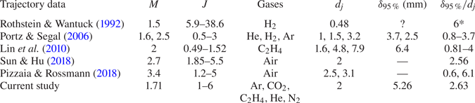
As described in § 2.2, the jet trajectories in this study are determined using mean jet fluid signals derived from Mie-scattering results. The actually measured quantity is the jet fluid signal, $( \rho \cdot f )$ and not the pure mixture fraction $f$, especially in regions of significant dilatation effects. The trajectories reported are defined as the 2 % jet fluid signal iso-contour on the windward side of the jet. The nominal flow conditions for all trajectories considered in this section are summarized in table 6. All of the current study's results are displayed after processing them with a third-order Savitzky–Golay filter to reduce spurious fluctuations.

Table 6.

Data sets used for trajectory comparison. In all cases, the trajectory is defined at the windward edge of the jet as some kind of mixture fraction or concentration iso-contour, with a threshold varying between 1 % and 10 %. For the current study, see the definition in § 2.2. For the other data sets, see table 4. For the entry marked with * no direct measurement is available, a reasonable value for $\delta _{95\,\%}/d_j$ was assumed based on the reported injector diameter, $d_j = 0.48$ mm, and the geometry of their test facility.

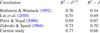
Two previously published empirical JISCF correlations by Rothstein & Wantuck (Reference Rothstein and Wantuck1992) and Lin et al. (Reference Lin, Ryan, Carter, Gruber and Raffoul2010) are shown first, in figures 16 and 17, respectively. For consistent comparison, the scalings are adjusted to include the $J^{{1}/{2}} d_j$ normalization of the $x$-coordinate. The scaling by Rothstein & Wantuck (Reference Rothstein and Wantuck1992) (figure 16) is more effective at collapsing the trajectory data than the one by Lin et al. (Reference Lin, Ryan, Carter, Gruber and Raffoul2010). The data sets by Pizzaia & Rossmann (Reference Pizzaia and Rossmann2018) are an exception, but that is not too surprising as they are the only ones reported for normalized jet fluid signal values and significant variation in the boundary layer effects $\delta /d_j$. However, the Pizzaia & Rossmann (Reference Pizzaia and Rossmann2018) data sets also show clearly that the Rothstein & Wantuck (Reference Rothstein and Wantuck1992) scaling does not explicitly consider differences in $\delta /d_j$, i.e. the Pizzaia & Rossmann (Reference Pizzaia and Rossmann2018) trajectories cluster by $\delta /d_j$ values, with the higher $\delta /d_j$ cases lying around $y/d_j/J_1^{0.4165} \approx 5$ and the thinner boundary layer cases lying around $y/d_j/J_1^{0.4165} \approx 3.5$.

Figure 16.

Trajectory collapse using the correlation reported by Rothstein & Wantuck (Reference Rothstein and Wantuck1992); dotted line (blue) Pizzaia & Rossmann (Reference Pizzaia and Rossmann2018), solid line with rectangle (purple) Sun & Hu (Reference Sun and Hu2018), circle (black) Lin et al. (Reference Lin, Ryan, Carter, Gruber and Raffoul2010), $\times$ (green) Portz & Segal (Reference Portz and Segal2006), dash-dotted line (orange) Rothstein & Wantuck (Reference Rothstein and Wantuck1992), dashed line (red) current study, solid line (black) power-law curve fit.

Figure 17.

Trajectory collapse using the correlation reported by Lin et al. (Reference Lin, Ryan, Carter, Gruber and Raffoul2010); dotted line (blue) Pizzaia & Rossmann (Reference Pizzaia and Rossmann2018), solid line with rectangle (purple) Sun & Hu (Reference Sun and Hu2018), circle (black) Lin et al. (Reference Lin, Ryan, Carter, Gruber and Raffoul2010), $\times$ (green) Portz & Segal (Reference Portz and Segal2006), dash-dotted line (orange) Rothstein & Wantuck (Reference Rothstein and Wantuck1992), dashed line (red) current study, solid line (black) power-law curve fit.

For a more quantitative comparison of the effectiveness of different scalings, the coefficient of determination, $R^2$, is computed and summarized in table 7. The value of $R^2$ is a measure of the variance in a dependent variable that can be predicted from the independent variable. Thus, a higher $R^2$ value for a given trajectory scaling corresponds to a better correlation of the data points by that scaling.

Table 7.

Coefficient of determination computed for the different correlations and scalings investigated. Only the Pizzaia & Rossmann (Reference Pizzaia and Rossmann2018) data set is excluded from the computation due to the differing trajectory definition. Both $x$-scalings involving $J^{{1}/{2}}$ and $J$ are considered.

Trajectory collapse for the Portz & Segal (Reference Portz and Segal2006) correlation is shown in figure 18. Based on the $R^2$ value in table 7 it performs slightly worse than the Rothstein & Wantuck (Reference Rothstein and Wantuck1992) result. However, it does seem to account for changes in $\delta /d_j$, as evident in the improved collapse of the Pizzaia & Rossmann (Reference Pizzaia and Rossmann2018) data. An attempt was made to use $J_2$ in the Portz & Segal (Reference Portz and Segal2006) correlation but it worsened the $R^2$ score significantly, probably due to the fact that it is a purely empirical correlation that was derived for usage with $J_1$.

Figure 18.

Trajectory collapse using the correlation reported by Portz & Segal (Reference Portz and Segal2006); dotted line (blue) Pizzaia & Rossmann (Reference Pizzaia and Rossmann2018), solid line with rectangle (purple) Sun & Hu (Reference Sun and Hu2018), circle (black) Lin et al. (Reference Lin, Ryan, Carter, Gruber and Raffoul2010), $\times$ (green) Portz & Segal (Reference Portz and Segal2006), dash-dotted line (orange) Rothstein & Wantuck (Reference Rothstein and Wantuck1992), dashed line (red) current study, solid line (black) power-law curve fit.

In figure 19, the trajectory collapse using the scaling of Zukoski & Spaid (Reference Zukoski and Spaid1964) ((1.4)) is considered. This entirely analytic scaling, devoid of any empirical constants, works well both qualitatively and quantitatively in comparison to scalings shown so far. In terms of $R^2$, it performs almost as well as the Rothstein & Wantuck (Reference Rothstein and Wantuck1992) correlation. Thus, a scaling approach based on the momentum balance between cross-flow and jet yields promising results. A discernible shortcoming is the missing consideration of boundary layer effects, as evidenced by the spread in the Pizzaia & Rossmann (Reference Pizzaia and Rossmann2018) data.

Figure 19.

Trajectory collapse using the scaling factor reported by Zukoski & Spaid (Reference Zukoski and Spaid1964); dotted line (blue) Pizzaia & Rossmann (Reference Pizzaia and Rossmann2018), solid line with rectangle (purple) Sun & Hu (Reference Sun and Hu2018), circle (black) Lin et al. (Reference Lin, Ryan, Carter, Gruber and Raffoul2010), $\times$ (green) Portz & Segal (Reference Portz and Segal2006), dash-dotted line (orange) Rothstein & Wantuck (Reference Rothstein and Wantuck1992), dashed line (red) current study, solid line (black) power-law curve fit.

The results for the semi-empirical scaling developed in § 3.2.1, i.e. $x/(J_2^{1/2} d_j)$ and $y/d_j/(h_c/d_j)$, are presented in figure 20. The curve fit constants for (3.10) are $A = 0.886$, $B = 0.235$ and $C=-0.492$. Close to the jet orifice, the curve fit is biased towards the data collected for this study, due to the low number of data points available in this area from other studies. Qualitatively, the collapse of all jet trajectories considered is good. The scaling appears to capture boundary layer effects successfully, as evidenced by the collapse of the Pizzaia & Rossmann (Reference Pizzaia and Rossmann2018) data. It collapses trajectories close to a value of $y/d_j/(h_c/d_j) \approx 1$. Quantitatively, out of all approaches considered, the developed scaling has the highest $R^2$ value, see table 7, however, the improvement over the empirical Rothstein & Wantuck (Reference Rothstein and Wantuck1992) correlation and the analytical Zukoski & Spaid (Reference Zukoski and Spaid1964) scaling is small. The new scaling captures between 1 % and 5 % more of the variance in the data sets used for comparison. For all scaling approaches considered, using $J$ instead of $J^{{1}/{2}}$ clearly deteriorates the $R^2$ values in table 7, even when all other parameters are adjusted appropriately. Thus, in this particular study, $J^{{1}/{2}}$ is the more relevant $x$-coordinate scaling parameter. Part of the remaining variability between trajectories can be attributed to differences in trajectory definition, diagnostics used (see table 4), the way in which the jet origin is reported, entrainment/mixing differences between injectants, and experimental uncertainty. That the Pizzaia & Rossmann (Reference Pizzaia and Rossmann2018) data collapse relatively well with all the other trajectories should be regarded as fortuitous, since the corresponding trajectory definition is very different. The specific influence of injectant properties is discussed in more detail later.

Figure 20.

JISCF mean trajectories scaled with the $h_c$ parameter presented in this study. The collapse is significantly improved for the entire range of momentum flux ratios, Mach numbers, jet injectants and boundary layer thicknesses; dotted line (blue) Pizzaia & Rossmann (Reference Pizzaia and Rossmann2018), solid line with rectangle (purple) Sun & Hu (Reference Sun and Hu2018), circle (black) Lin et al. (Reference Lin, Ryan, Carter, Gruber and Raffoul2010), $\times$ (green) Portz & Segal (Reference Portz and Segal2006), dash-dotted line (orange) Rothstein & Wantuck (Reference Rothstein and Wantuck1992), dashed line (red) current study, solid line (black) power-law curve fit.

The relative success of the newly presented scaling supports the notion that the effective momentum flux ratio, computed after a normal shock ($J_2$ in (1.6)), might be more relevant for the problem than the global pre-shock momentum flux ratio $J$ or $J_1$. The comparison of $R^2$ values for different correlations, in table 7, also confirms that the most dominant parameter for mean jet trajectory development is the momentum flux ratio. Thus, the newly developed scaling is particularly useful for cases in which a thick boundary layer is present and $J_1$ is relatively low ($1 \leq J \leq 6$). For higher values of $J_1$ and thin boundary layers, the empirical Rothstein & Wantuck (Reference Rothstein and Wantuck1992) correlation and the analytical Zukoski & Spaid (Reference Zukoski and Spaid1964) scaling are sufficient.

The results also suggest two important practical considerations. One, the momentum balance approach captures at least part of the physics relevant for determining the jet trajectory evolution. Two, deriving an empirical trajectory correlation from data at relatively high $J$ values yields a more generalizable result (see the Rothstein & Wantuck (Reference Rothstein and Wantuck1992) conditions in table 6 and the results in figure 16). Our proposed scaling has the advantage of explicitly considering flow field features controlling the jet trajectory, i.e. the bow shock and the velocity boundary layer. Thus, using the new scaling, it is easier to investigate further parameters’ effects on the jet trajectory and potentially extend the model to account for those. Data points with $J < 0.5$ have been excluded from the current jet trajectory analysis as they do not collapse with the other data points. Given that the current formulation of $h_c$ emphasizes the importance of the momentum flux reduction in both cross-flow and jet, it is likely that such barely choked jets do not result in the required shock strengths for the scaling to work. This is in contrast to the model developed by Heister & Karagozian (Reference Heister and Karagozian1990) for perfectly expanded and barely underexpanded jets. Combining this model with the presented scaling could yield impactful results.

The prominent importance of the momentum flux ratio, especially at higher $J$ (see scaling of Rothstein & Wantuck (Reference Rothstein and Wantuck1992) in figure 16), motivates a simplification of the proposed scaling parameter, $h_c$ (suggested by a reviewer). This simplification provides a decent engineering estimate and is made at the expense of losing explicit flow field physics representation. Assuming that $\delta < \delta _s$ at large $J$, a reasonable assumption for thin supersonic boundary layers, one can write a simplified characteristic penetration as,

(3.11)

\begin{equation} \frac{h_c'}{d_j} = C_h' J_2^{{5}/{9}}. \end{equation}

All of the constant values, the calibration constants, the weakly Mach number dependent drag coefficient and shock angle, $\beta$, are lumped together into one calibration constant, $C'$, in this expression. The analytically derived exponent value of $5/9$ is approximately 33 % higher than the empirical measurement of $0.4165$ by Rothstein & Wantuck (Reference Rothstein and Wantuck1992). Performing the multi-parameter curve fit described in § 3.2.1 yields $C_h' = 1.43$ and $R^2 = 0.73$, compared to $R^2 = 0.89$ for the full scaling expression of $h_c$. See figure 15 for the resulting fit surface and figure 21 for the resulting trajectory collapse.

Figure 21.

Trajectory collapse using a simplified $h_c'$ scaling parameter for engineering estimates; dotted line (blue) Pizzaia & Rossmann (Reference Pizzaia and Rossmann2018), solid line with rectangle (purple) Sun & Hu (Reference Sun and Hu2018), circle (black) Lin et al. (Reference Lin, Ryan, Carter, Gruber and Raffoul2010), $\times$ (green) Portz & Segal (Reference Portz and Segal2006), dash-dotted line (orange) Rothstein & Wantuck (Reference Rothstein and Wantuck1992), dashed line (red) current study, solid line (black) power-law curve fit.

Confidence intervals for this study's trajectories are shown in figures 22 and 23. The intervals are computed as described in appendix A. In the normalized $y$-direction, the confidence intervals are relatively small and limited to intervals of approximately $\pm 0.25 y/d_j/(h_c/d_j)$. Uncertainties in the normalized $x$-direction grow slowly with downstream distance up to a maximum interval size of approximately $\pm 0.12 x/J_2^{{1}/{2}}d_j$.

Figure 22.

Visualization of uncertainties in this study's jet trajectory data and influence of $\gamma$ on penetration. Lines are the trajectories reported, grey bands are uncertainties in the $y$-coordinate and black dots with horizontal lines are uncertainties in the $x$-coordinate at every 40th data point. Solid line (red) $\gamma = 1.66$ ($\mathrm {Ar}$ and $\mathrm {He}$), dotted line (green) $\gamma = 1.4$ ($\mathrm {N_2}$), dashed line (blue) $\gamma = 1.28\ {\rm and}\ 1.237$ ($\mathrm {CO_2}$ and $\mathrm {C_2 H_4}$).

Figure 23.

Visualization of uncertainties in this study's jet trajectory data and influence of $MW$ on penetration. Lines are the trajectories reported, grey bands are uncertainties in the $y$-coordinate and black dots with horizontal lines are uncertainties in the $x$-coordinate at every 40th data point. solid line (red) $MW \approx 40$ g mol$^{-1}$ ($\mathrm {Ar}$ and $\mathrm {CO_2}$), dotted line (green) $MW \approx 28$ g mol$^{-1}$ ($\mathrm {C_2 H_4}$ and $\mathrm {N_2}$), dashed line (blue) $MW = 4$ g mol$^{-1}$ ($\mathrm {He}$).

Trajectories in figures 22 and 23 are marked to emphasize the effect of varying jet fluid specific heat ratio and molecular weight, respectively. Close to the jet orifice, the jet fluid properties ($MW$ and $\gamma$) do not seem to have a discernible effect on the mean trajectory. Downstream of the jet bending point, however, the scatter between trajectories increases. The effect of $\gamma$ on normalized penetration in figure 22 is weak and suggests that higher $\gamma$ leads to slightly higher penetration and later drop offs in the 2 % jet fluid signal iso-contour. Moreover, two of the lower $MW$ gases used, helium and ethylene, exhibit higher penetration and later drop off of the iso-contour than the higher $MW$ gases used, argon and carbon dioxide, see figure 23. This trend becomes clearer the farther downstream one moves along the jet.

Because the trajectories are defined along absolute jet fluid signal iso-contours, and recalling the discussion in § 2.3, the observations could imply that gases with lower specific heat ratios mix faster with the cross-flow than gases with higher specific heat ratios. These results generally agree with the conclusions in Gruber et al. (Reference Gruber, Nejad, Chen and Dutton1997a), Ben-Yakar et al. (Reference Ben-Yakar, Mungal and Hanson2006) and Takahashi et al. (Reference Takahashi, Masuya and Hirota2010). They are also supported by the convective Mach number results of Papamoschou & Roshko (Reference Papamoschou and Roshko1988) and Gruber et al. (Reference Gruber, Nejad, Chen and Dutton1997a), where lower $MW$ gases cause a higher convective Mach number, which suppresses hydrodynamic instability growth and entrainment.

In figure 24, the focus is on the nitrogen, ethylene and helium cases. Again, the overall influence of injectant properties appear small. Nonetheless, trends are discernible. Except for $J=1$, the ethylene trajectories all drop off faster than the corresponding nitrogen trajectories. This suggests that the higher $\gamma$ of nitrogen causes a reduction in entrainment and turbulent mixing rates, since its $MW$ is almost identical to that of ethylene. At $J=1$ the nitrogen and ethylene trajectory evolve closer together, i.e. at this low momentum flux ratio, the suppression of hydrodynamic instabilities might be relatively equal for the two injectants, see figure 13(a).

Figure 24.

Close up of nitrogen and helium trajectories; dashed line (green) $\mathrm {N_2}$ with $MW = 28$ g mol$^{-1}$ and $\gamma = 1.4$, dashed line (blue) $\mathrm {C_2 H_4}$ with $MW \approx 28$ g mol$^{-1}$ and $\gamma = 1.237$, dashed line (red) $\mathrm {He}$ with $MW = 4$ g mol$^{-1}$ and $\gamma = 1.66$. $\bullet \ J=1$, $\blacksquare \ J=2$, $\blacktriangle \ J=4$, $\blacklozenge \ J=6$.

Ethylene also appears to mix faster than the helium jets at all $J$. Interestingly, the nitrogen trajectories penetrate deeper than the helium trajectories for $J>1$. This seems to contradict the notion that higher $MW$ injectants should entrain and mix faster. However, there are two logical explanations for this behaviour. One, the helium and nitrogen trajectories exhibit very similar penetration overall, i.e. the nitrogen cases penetrating deeper could be an artefact of experimental uncertainty. For the other explanation, the discussion of jet fluid signal iso-contour behaviour in § 2.3 is recalled. Then, the nitrogen trajectories penetrating deeper than helium can be interpreted as nitrogen having a larger turbulent mixing rate than helium, but not as high as ethylene, so that the drop-off point in the trajectory is not reached in the experimental field of view for $J>1$. The latter point also implying that, for the presented data, nitrogen has a relatively low turbulent mixing rate overall. Only helium mixes even slower.

In figures 22 and 23, both the highest $MW$ gases, argon and carbon dioxide, do not penetrate as deep as nitrogen and reach earlier drop-off points in their trajectories, at all $J$. Thus, supporting the claim that the observed behaviour of the nitrogen trajectories is indeed due to turbulent mixing rates, and not experimental uncertainties.

4. Conclusions

We acquired and presented JISCF Mie-scattering data for five different injectants at four momentum flux ratios. Mean and r.m.s. fluctuating jet fluid signals are analysed, with an emphasis on the influence of jet molecular weight and specific heat ratio on turbulent mixing. We also developed a new scaling for the mean jet trajectory of gaseous, underexpanded sonic jets in a supersonic cross-flow. The scaling considers the momentum flux reduction of the cross-flow, caused by the boundary layer and the jet bow shock, to be controlling factors for the mean evolution of the jet in the near field. To validate the scaling, we extracted mean jet trajectories from our Mie-scattering results and included data from four other studies for comparison. Thus, the analysis covers variations in the momentum flux ratio, the molecular weight and specific heat ratio of the injectants, the cross-flow Mach number, the boundary layer thickness and the jet exit diameter. The range of injectant properties reported in this study is an important addition to the existing body of knowledge on JISCF.

The mean jet fluid signals indicate that turbulent mixing processes can change with injectant molecular weight and specific heat ratio. The fluctuating component of the jet fluid signal reveals that, at higher momentum flux ratios ($J = 4\text {--}6$) and for the current experimental set-up, the convective Mach number concept can predict the observed behaviour. However, at lower momentum flux ratios ($J < 4$), the observed distribution and magnitude of jet fluid signal fluctuations are the opposite of what would be expected purely from the convective Mach number concept. We suggest that the stronger interaction with the boundary layer at lower momentum flux ratios plays an important role, causing the observed change with $MW$ and $J$. Moreover, we conjecture that the magnitude of the convective Mach number changes more strongly with $J$ for the lower $MW$ gases than the high $MW$ gases. Calculations from a simple analytical model support this conjecture, but direct measurements of the JISCF pressure field or of jet shear layer convective velocities, as a function of $J$, are required to really put it to the test. Practically, the findings imply that optimizing turbulent mixing requires the consideration of boundary layer, jet operating point and injectant properties, simultaneously. On a very high level, the jet sonic velocity is a qualitative indicator of turbulent mixing rates. For a low $MW$ gas, a low momentum flux ratio and thicker boundary layer can be beneficial to maximize turbulent mixing. For higher $MW$ gases, a higher momentum flux ratio and thinner boundary layer can yield better results.

For all data sets considered, the newly developed scaling improves the collapse of mean jet trajectories over previous attempts, especially in the near field of the jet. Quantitatively, based on a measure of $R^2$, the developed scaling shows a decent improvement (${\sim }1\,\%\text {--}51\,\%$) over all other empirical and analytical approaches examined. Besides two calibration constants and an expression for the jet drag coefficient, the scaling is analytical and requires no curve-fit expressions. The explicit consideration of flow physics in the scaling makes further testing, extension and modification relatively simple. The results show that the developed scaling is particularly useful at lower momentum flux ratios (e.g. in this study $J\leq 6$) and in the presence of thick boundary layers. For high enough $J$ and thin boundary layers, the momentum flux ratio dominates and the boundary layer and bow shock changes play a secondary role. Based on this analysis, a simplified trajectory law for engineering estimates is presented, yielding similarly high correlation values for all data sets. Further analysis suggests that higher $MW$ injectants with lower specific heat ratios generally exhibit lower penetration (i.e. potentially faster turbulent mixing). The influence of molecular weight and specific heat ratio can be anticipated from literature results and the convective Mach number concept. The influence of the specific heat ratio, however, has not been shown explicitly outside this study. One limitation of the new scaling is that it does not work for momentum flux ratios below one.

Our future research will focus on explicitly testing the conjecture made for the rate of change of the convective Mach number with momentum flux ratio. Moreover, while the jet trajectory scaling works reasonably well in its current form, it could be improved by finding a more accurate effective drag coefficient, by understanding the jet to bow shock relationship better and by extending it to $J < 1$ jets.

Supplementary material

Supplementary material are available at https://doi.org/10.1017/jfm.2020.1065.

Acknowledgements

The first author would like to acknowledge the very useful discussions with Professor A. Steinberg.

Funding

The authors acknowledge partial support of this study by AFOSR (grant number FA9550-15-1-0512) and the DOE (grant number DE-FOA-0001386).

Declaration of interest

The authors report no conflict of interest.

Appendix A

The total statistical uncertainty of jet trajectories based on jet fluid signal contours is computed via basic uncertainty propagation principles (Coleman & Steele Reference Coleman and Steele2009) and estimates of statistical confidence intervals (for a 95 % confidence level) where appropriate. Unless otherwise stated, we assume that confidence intervals can be estimated assuming a normal distribution for the quantity of interest. Since at least 900 samples are available for any computed quantity, this is a reasonable assumption.

For the $x$-coordinate the following sources of uncertainty are considered: cross-flow Mach number, cross-flow stagnation pressure and jet stagnation pressure. The resulting uncertainty is,

(A1)

\begin{equation} U^2_{x/J_2^{0.5}d_j} = \left( \frac{\partial}{\partial J_2} \left( \frac{x}{J_2^{0.5}d_j} \right)U_{J_2} \right)^2. \end{equation}

With,

(A2)

\begin{equation} U_{J_2}^2 = \left( \frac{\partial J_2}{\partial J_1} U_{J_1} \right)^2 + \left( \frac{\partial J_2}{\partial M_{\infty,1}} \sigma_{M_{\infty,1}} \right)^2. \end{equation}

Where $\sigma _{M_{\infty ,1}} = 0.06$ from the static wall pressure measurements in § 2.1 is used and,

(A3)

\begin{equation} U^2_{J_1} = \left( \frac{\partial J_1}{\partial p_{0,\infty}} \sigma_{p_{0,\infty}} \right)^2 + \left( \frac{\partial J_1}{\partial p_{0,j}} \sigma_{p_{0,j}} \right)^2 + \left( \frac{\partial J_1}{\partial M_{\infty,1}} \sigma_{M_{\infty,1}} \right)^2. \end{equation}

The cross-flow stagnation pressure uncertainty is the combined measurement and run uncertainty, $\sigma _{p_{0,\infty }} \approx 9.4$ kPa, as is the jet stagnation pressure uncertainty $\sigma ^2_{p_{0,j}} = ( U_{meas}(p_{0,\infty }) )^2 + ( 1.96 \sigma _{p_{0,\infty }}/\sqrt {n} )^2$, where U _meas is the measurement uncertainty, $n$ is the number of samples (here always $>900$) and the first term is determined via the pressure transducer calibration.

For the $y$-coordinate the statistical uncertainty in the position of the 2 % trajectory itself, uncertainties in the boundary layer thickness measurement, and the correlation between uncertainties in the 2 % trajectory position and uncertainties in the post-shock momentum flux ratio are considered in addition. A correlation coefficient of $\rho ' = 1$ is assumed between $y$ and $J_2$, both as a worst-case estimate and because the two quantities are generally strongly correlated. This yields the following expression:

(A4)

\begin{equation} U^2_{y/h_c} = \left( \frac{\partial y/h_c}{\partial J_2} U_{J_2} \right)^2 + \left( \frac{\partial y/h_c}{\partial y} \sigma_y \right)^2 + \left( \frac{\partial y/h_c}{\partial \delta} \sigma_{\delta} \right)^2 + 2 \frac{\partial y/h_c}{\partial y} \frac{\partial y/h_c}{\partial J_2} \rho' \sigma_y U_{J_2}. \end{equation}

The uncertainty of the trajectory position is estimated using the $y$-derivative of the mean jet fluid signal field and the jet fluid signal standard deviation in the following way:

(A5)

\begin{equation} \sigma_y = \frac{1.96}{\sqrt{N}} \left[\frac{\textrm{d} y}{d(\overline{\rho f})} \sigma_{(\overline{\rho f})}\right]_{\overline{\rho f} = 0.02}. \end{equation}

The uncertainty of the boundary layer thickness is estimated in a similar fashion assuming a linear velocity profile yielding,

(A6)

\begin{equation} \sigma_\delta = \left.\frac{1.96}{\sqrt{N}} \frac{\delta_{95\,\%}}{u_\infty} \sigma_u \right|_{\delta_{95\,\%}} \approx 0.02 \ \mathrm{mm}. \end{equation}

The statistical uncertainty of the mean jet fluid signal field is simply estimated as,

(A7)

\begin{equation} U^2_{\overline{\rho f}} = 1.96^2 \frac{\sigma_{\rho f}^2}{N} . \end{equation}

This assumes that fluctuations in $f$ and $\rho$, due to changes in the cross-flow and jet conditions, are all quantified sufficiently by the standard deviation of the jet fluid signal field itself.

Similarly the statistical uncertainty of the r.m.s. jet fluid signal fluctuation evaluates to this simple relationship,

(A8)

\begin{equation} U^2_{\sqrt{\overline{(\rho f)'^2}}} = 1.96^2 \frac{\overline{(\rho f)'^2}}{2 N}. \end{equation}

References

REFERENCES

Anderson, J.D. 2006 Hypersonic and High-Temperature Gas Dynamics. AIAA.10.2514/4.861956CrossRef Google Scholar

Ben-Yakar, A., Mungal, M.G. & Hanson, R.K. 2006 Time evolution and mixing characteristics of hydrogen and ethylene transverse jets in supersonic crossflows. Phys. Fluids 18 (2), 026101.10.1063/1.2139684CrossRef Google Scholar

Bertagni, M.B., Marro, M., Salizzoni, P. & Camporeale, C. 2019 Solution for the statistical moments of scalar turbulence. Phys. Rev. Fluids 4 (12), 124701.10.1103/PhysRevFluids.4.124701CrossRef Google Scholar

Broadwell, J.E. & Breidenthal, R.E. 1984 Structure and mixing of a transverse jet in incompressible flow. J. Fluid Mech. 148, 405–412.10.1017/S0022112084002408CrossRef Google Scholar

Castellanos, J.L., Gómez, S. & Guerra, V. 2002 The triangle method for finding the corner of the l-curve. Appl. Numer. Maths 43 (4), 359–373.10.1016/S0168-9274(01)00179-9CrossRef Google Scholar

Chauhan, K.A., Monkewitz, P.A. & Nagib, H.M. 2009 Criteria for assessing experiments in zero pressure gradient boundary layers. Fluid Dyn. Res. 41 (2), 021404.10.1088/0169-5983/41/2/021404CrossRef Google Scholar

Coleman, H.W. & Steele, W.G. 2009 Experimentation, Validation, and Uncertainty Analysis for Engineers. John Wiley & Sons.10.1002/9780470485682CrossRef Google Scholar

Gamba, M. & Mungal, M.G. 2015 Ignition, flame structure and near-wall burning in transverse hydrogen jets in supersonic crossflow. J. Fluid Mech. 780, 226–273.10.1017/jfm.2015.454CrossRef Google Scholar

Gevorkyan, L., Shoji, T., Getsinger, D.R., Smith, O.I. & Karagozian, A.R. 2016 Transverse jet mixing characteristics. J. Fluid Mech. 790, 237–274.10.1017/jfm.2016.5CrossRef Google Scholar

Gruber, M.R., Nejadt, A.S., Chen, T.H. & Dutton, J.C. 1995 Mixing and penetration studies of sonic jets in a mach 2 freestream. J. Propul. Power 11 (2), 315–323.10.2514/3.51427CrossRef Google Scholar

Gruber, M.R., Nejad, A.S., Chen, T.H. & Dutton, J.C. 1997 a Compressibility effects in supersonic transverse injection flowfields. Phys. Fluids 9 (5), 1448–1461.10.1063/1.869257CrossRef Google Scholar

Gruber, M.R., Nejad, A.S., Chen, T.H. & Dutton, J.C. 1997 b Large structure convection velocity measurements in compressible transverse injection flowfields. Exp. Fluids 22 (5), 397–407.10.1007/s003480050066CrossRef Google Scholar

Gruber, M.R., Nejad, A.S., Chen, T.H. & Dutton, J.C. 2000 Transverse injection from circular and elliptic nozzles into a supersonic crossflow. J. Propul. Power 16 (3), 449–457.10.2514/2.5609CrossRef Google Scholar

Hasselbrink, E.F. & Mungal, M.G. 2001 Transverse jets and jet flames. Part 1. Scaling laws for strong transverse jets. J. Fluid Mech. 443, 1–25.10.1017/S0022112001005146CrossRef Google Scholar

Heister, S.D. & Karagozian, A.R. 1990 Gaseous jet in supersonic crossflow. AIAA J. 28 (5), 819–827.10.2514/3.25125CrossRef Google Scholar

Lin, K., Ryan, M., Carter, C., Gruber, M. & Raffoul, C. 2010 Raman scattering measurements of gaseous ethylene jets in a mach 2 supersonic crossflow. J. Propul. Power 26 (3), 503–513.10.2514/1.43757CrossRef Google Scholar

Mahesh, K. 2013 The interaction of jets with crossflow. Annu. Rev. Fluid Mech. 45, 379–407.10.1146/annurev-fluid-120710-101115CrossRef Google Scholar

McClinton, C.R. 1974 Effect of ratio of wall boundary layer thickness to jet diameter on mixing of a normal hydrogen jet in a supersonic stream. Tech. Rep. NASA-TM-X-3030. NTRS, NASA Langley Research Center (US), Washington (DC), contract No.: RTOP 501-04-03-03.Google Scholar

McDaniel, J.C. & Raves, J. 1988 Laser-induced-fluorescence visualization of transverse gaseous injection in a nonreacting supersonic combustor. J. Propul. Power 4 (6), 591–597.10.2514/3.23105CrossRef Google Scholar

Muppidi, S. & Mahesh, K. 2005 Study of trajectories of jets in crossflow using direct numerical simulations. J. Fluid Mech. 530, 81–100.10.1017/S0022112005003514CrossRef Google Scholar

Papamoschou, D. & Hubbard, D.G. 1993 Visual observations of supersonic transverse jets. Exp. Fluids 14 (6), 468–476.10.1007/BF00190201CrossRef Google Scholar

Papamoschou, D. & Roshko, A. 1988 The compressible turbulent shear layer: an experimental study. J. Fluid Mech. 197, 453–477.10.1017/S0022112088003325CrossRef Google Scholar

Pernpeintner, M., Lauer, M., Hirsch, C. & Sattelmayer, T. 2011 A method to obtain planar mixture fraction statistics in turbulent flows seeded with tracer particles. In ASME 2011 Turbo Expo: Turbine Technical Conference, pp. 1341–1350. American Society of Mechanical Engineers Digital Collection.10.1115/GT2011-46844CrossRef Google Scholar

Pizzaia, A. & Rossmann, T. 2018 Effect of boundary layer thickness on transverse sonic jet mixing in a supersonic turbulent crossflow. Phys. Fluids 30 (11), 115104.10.1063/1.5056540CrossRef Google Scholar

Pope, S.B. 2000 Turbulent Flows. Cambridge University Press.10.1017/CBO9780511840531CrossRef Google Scholar

Portz, R. & Segal, C. 2006 Penetration of gaseous jets in supersonic flows. AIAA J. 44 (10), 2426–2429.10.2514/1.23541CrossRef Google Scholar

Povinelli, F.P., Povinelli, L.A. & Hersch, M. 1970 Supersonic jet penetration/up to mach 4/into a mach 2 airstream. J. Spacecr. Rockets 7 (8), 988–992.10.2514/3.30082CrossRef Google Scholar

Ragni, D., Schrijer, F., Van Oudheusden, B.W. & Scarano, F. 2011 Particle tracer response across shocks measured by PIV. Exp. Fluids 50 (1), 53–64.10.1007/s00348-010-0892-2CrossRef Google Scholar

Rothstein, A. & Wantuck, P. 1992 A study of the normal injection of hydrogen into a heated supersonicflow using planar laser-induced fluorescence. In 28th Joint Propulsion Conference and Exhibit, Nashville, TN, July 6–8. AIAA, SAE, ASME, and ASEE.10.2514/6.1992-3423CrossRef Google Scholar

Santiago, J.G. & Dutton, J.C. 1997 Velocity measurements of a jet injected into a supersonic crossflow. J. Propul. Power 13 (2), 264–273.10.2514/2.5158CrossRef Google Scholar

Sautet, J.C. & Stepowski, D. 1994 Single-shot laser Mie scattering measurements of the scalar profiles in the near field of turbulent jets with variable densities. Exp. Fluids 16 (6), 353–367.10.1007/BF00202058CrossRef Google Scholar

Smith, S.H. & Mungal, M.G. 1998 Mixing, structure and scaling of the jet in crossflow. J. Fluid Mech. 357, 83–122.10.1017/S0022112097007891CrossRef Google Scholar

Sun, M. & Hu, Z. 2018 Mixing in nearwall regions downstream of a sonic jet in a supersonic crossflow at mach 2.7. Phys. Fluids 30 (10), 106102.10.1063/1.5045752CrossRef Google Scholar

Takahashi, H., Masuya, G. & Hirota, M. 2010 Effects of injection and main flow conditions on supersonic turbulent mixing structure. AIAA J. 48 (8), 1748–1756.10.2514/1.J050355CrossRef Google Scholar

VanLerberghe, W.M., Santiago, J.G., Dutton, J.C. & Lucht, R.P. 2000 Mixing of a sonic transverse jet injected into a supersonic flow. AIAA J. 38 (3), 470–479.10.2514/2.984CrossRef Google Scholar

Watanabe, J., Kouchi, T., Takita, K. & Masuya, G. 2012 Large-eddy simulation of jet in supersonic crossflow with different injectant species. AIAA J. 50 (12), 2765–2778.10.2514/1.J051550CrossRef Google Scholar

White, F.M. & Corfield, I. 2006 Viscous Fluid Flow, vol. 3. McGraw-Hill.Google Scholar

Zukoski, E.E. & Spaid, F.W. 1964 Secondary injection of gases into a supersonic flow. AIAA J. 2 (10), 1689–1696.10.2514/3.2653CrossRef Google Scholar

Figure 1.(a) Schematic of the JISCF centreline flow field with the dominant features of interest for this study. (b) Schematic of the flow field processes and velocity profiles relevant to the developed momentum deficit scaling. The dashed line along the bow shock corresponds to the velocity profile on the right.

Table 1.Sample of studies reporting JISCF trajectories.

Table 2.Coefficients for (1.7).

Figure 2.Schematic of the experimental facility used to obtain the presented measurements. The green block in the test section is the injector.

Table 3.Properties of gases used for injection and design ranges of nominal mass flow rates and jet Reynolds numbers, $Re_d = \frac{U_j d_j}{\nu_j} $ at the orifice. Entries marked with * depend strongly on temperature, the values reported here are representative at room temperature.

Figure 3.Wall pressure measurements and Mach number distribution. The $x$-axis is normalized by the test section height, $H=8$ cm, and measured from the beginning of the test section. The green solid line is the nozzle design condition/Mach number. The dashed vertical line is the location of the injector on the bottom of the test section. The other dashed horizontal lines represent pressures and Mach numbers at ${\rm \Delta} M = 0.05$ intervals. (a) Static wall pressure normalized by the stagnation pressure. In the nozzle the pressures are measured on the side wall, in the test section they are measured on the top wall. (b) Mach number distribution computed via isentropic expansion relations.

Figure 4.(a) Comparison of our supersonic boundary layer profile, after applying the van Driest transformation, to theory and experimental results by Pizzaia & Rossmann (2018). The presented velocity profile is extracted at the jet centreline location. Velocity uncertainty is below 3 % at a 95 % confidence level for the entire boundary layer profile. (b) Streamwise development of the 95 % boundary layer thickness. Also shown is the expected turbulent boundary layer growth assuming a $1/7$ power-law velocity profile (White & Corfield 2006). Shaded areas indicate the uncertainty of the boundary layer thickness. The dashed vertical line denotes the location of the jet orifice.

Figure 5.Optical set-up for Mie-scattering experiments.

Figure 6.Jet trajectory determination exemplified with $\mathrm {N_2}$$J=6$ data. From (a–c): instantaneous Mie-scattering image (after flatfield correction, median filtering and Gaussian filtering), mean image after the numerical inversion procedure and mean image overlayed with the two relevant trajectories determined via the iterative procedure: the maximum jet fluid signal (blue) and the 2 % jet fluid signal trajectory (green). For the trajectories both the actual data (circles) as well as power-law curve fits (solid lines) are shown.

Table 4.Brief survey of different jet penetration/trajectory definitions in the literature. ‘Norm?’ refers to whether the concentration profiles are re-normalized by the local maximum concentration value. The asterisk denotes ambiguity in the definition if it is based on qualitative markers or burning regions.

Figure 7.Examples of the two different approaches with which concentration iso-contour based jet penetrations (or jet trajectories) are determined in JISCF literature. The threshold here is $C = 0.05$. The black concentration profiles are plotted proportional to the $x$-coordinate and only for the lower $\sigma$ growth rate of $a = 0.2$. (a) Concentration iso-contours of a Gaussian mixing process. The growth rate $a$ of the profile spread $\sigma$ controls when the $y$-coordinate starts reducing again after the initial growth. (b) Concentration iso-contours of a Gaussian mixing process for which the profiles at each $x$-coordinate have been normalized by the centreline concentration. The growth rate $a$ of the profile spread $\sigma$ determines how fast the $y$-coordinate of the iso-contour grows.

Table 5.Targeted $J$ values and measured $J$ values for each gas used in the presented study.

Figure 8.Jet fluid signal results for argon. The nominal momentum flux ratio is indicated in the upper left corner. The black solid line is the corresponding 2 % jet trajectory. (a) Mean mixture fraction for argon. (b) The r.m.s. jet fluid signal for argon.

Figure 9.Jet fluid signal results for ethylene. The nominal momentum flux ratio is indicated in the upper left corner. The black solid line is the corresponding 2 % jet trajectory. The $J=6$ case had to be processed with a stronger Gaussian filter, than the other cases, to achieve convergence in the solution of the inverse problem yielding the jet fluid signal field. (a) Mean mixture fraction for ethylene. (b) The r.m.s. jet fluid signal for ethylene.

Figure 10.Jet fluid signal results for carbon dioxide. The nominal momentum flux ratio is indicated in the upper left corner. The black solid line is the corresponding 2 % jet trajectory. (a) Mean mixture fraction for carbon dioxide. (b) The r.m.s. jet fluid signal for carbon dioxide.

Figure 11.Jet fluid signal results for helium. The nominal momentum flux ratio is indicated in the upper left corner. The black solid line is the corresponding 2 % jet trajectory. (a) Mean mixture fraction for helium. (b) The r.m.s. jet fluid signal for helium.

Figure 12.Jet fluid signal results for nitrogen. The nominal momentum flux ratio is indicated in the upper left corner. The black solid line is the corresponding 2 % jet trajectory. (a) Mean mixture fraction for nitrogen. (b) The r.m.s. jet fluid signal for nitrogen.

Figure 13.Jet velocity estimates upstream of the Mach disk as a function of momentum flux ratio. Darker colours equal higher $MW$. (a) Jet velocity upstream of the Mach disk. (b) Jet velocity derivative with respect to momentum flux ratio.

Figure 14.Schlieren visualization of a $\mathrm {N_2}$ jet in a Mach 1.71 cross-flow. Top row $J = 2$, bottom row $J = 6$. Left column: instantaneous images, middle column: mean images, right column: r.m.s. images. Brighter colour corresponds to higher intensity values. Red lines mark flow field features of interest for the scaling developed here. The variations in the salient flow features with $J$ are clearly visible.

Figure 15.Results of curve fitting the expression in (3.5) to the empirical results of Portz & Segal (2006). Every 41st data point used for the curve fit is shown.

Table 6.Data sets used for trajectory comparison. In all cases, the trajectory is defined at the windward edge of the jet as some kind of mixture fraction or concentration iso-contour, with a threshold varying between 1 % and 10 %. For the current study, see the definition in § 2.2. For the other data sets, see table 4. For the entry marked with * no direct measurement is available, a reasonable value for $\delta _{95\,\%}/d_j$ was assumed based on the reported injector diameter, $d_j = 0.48$ mm, and the geometry of their test facility.

Figure 16.Trajectory collapse using the correlation reported by Rothstein & Wantuck (1992); dotted line (blue) Pizzaia & Rossmann (2018), solid line with rectangle (purple) Sun & Hu (2018), circle (black) Lin et al. (2010), $\times$ (green) Portz & Segal (2006), dash-dotted line (orange) Rothstein & Wantuck (1992), dashed line (red) current study, solid line (black) power-law curve fit.

Figure 17.Trajectory collapse using the correlation reported by Lin et al. (2010); dotted line (blue) Pizzaia & Rossmann (2018), solid line with rectangle (purple) Sun & Hu (2018), circle (black) Lin et al. (2010), $\times$ (green) Portz & Segal (2006), dash-dotted line (orange) Rothstein & Wantuck (1992), dashed line (red) current study, solid line (black) power-law curve fit.

Table 7.Coefficient of determination computed for the different correlations and scalings investigated. Only the Pizzaia & Rossmann (2018) data set is excluded from the computation due to the differing trajectory definition. Both $x$-scalings involving $J^{{1}/{2}}$ and $J$ are considered.

Figure 18.Trajectory collapse using the correlation reported by Portz & Segal (2006); dotted line (blue) Pizzaia & Rossmann (2018), solid line with rectangle (purple) Sun & Hu (2018), circle (black) Lin et al. (2010), $\times$ (green) Portz & Segal (2006), dash-dotted line (orange) Rothstein & Wantuck (1992), dashed line (red) current study, solid line (black) power-law curve fit.

Figure 19.Trajectory collapse using the scaling factor reported by Zukoski & Spaid (1964); dotted line (blue) Pizzaia & Rossmann (2018), solid line with rectangle (purple) Sun & Hu (2018), circle (black) Lin et al. (2010), $\times$ (green) Portz & Segal (2006), dash-dotted line (orange) Rothstein & Wantuck (1992), dashed line (red) current study, solid line (black) power-law curve fit.

Figure 20.JISCF mean trajectories scaled with the $h_c$ parameter presented in this study. The collapse is significantly improved for the entire range of momentum flux ratios, Mach numbers, jet injectants and boundary layer thicknesses; dotted line (blue) Pizzaia & Rossmann (2018), solid line with rectangle (purple) Sun & Hu (2018), circle (black) Lin et al. (2010), $\times$ (green) Portz & Segal (2006), dash-dotted line (orange) Rothstein & Wantuck (1992), dashed line (red) current study, solid line (black) power-law curve fit.

Figure 21.Trajectory collapse using a simplified $h_c'$ scaling parameter for engineering estimates; dotted line (blue) Pizzaia & Rossmann (2018), solid line with rectangle (purple) Sun & Hu (2018), circle (black) Lin et al. (2010), $\times$ (green) Portz & Segal (2006), dash-dotted line (orange) Rothstein & Wantuck (1992), dashed line (red) current study, solid line (black) power-law curve fit.

Figure 22.Visualization of uncertainties in this study's jet trajectory data and influence of $\gamma$ on penetration. Lines are the trajectories reported, grey bands are uncertainties in the $y$-coordinate and black dots with horizontal lines are uncertainties in the $x$-coordinate at every 40th data point. Solid line (red) $\gamma = 1.66$ ($\mathrm {Ar}$ and $\mathrm {He}$), dotted line (green) $\gamma = 1.4$ ($\mathrm {N_2}$), dashed line (blue) $\gamma = 1.28\ {\rm and}\ 1.237$ ($\mathrm {CO_2}$ and $\mathrm {C_2 H_4}$).

Figure 23.Visualization of uncertainties in this study's jet trajectory data and influence of $MW$ on penetration. Lines are the trajectories reported, grey bands are uncertainties in the $y$-coordinate and black dots with horizontal lines are uncertainties in the $x$-coordinate at every 40th data point. solid line (red) $MW \approx 40$ g mol$^{-1}$ ($\mathrm {Ar}$ and $\mathrm {CO_2}$), dotted line (green) $MW \approx 28$ g mol$^{-1}$ ($\mathrm {C_2 H_4}$ and $\mathrm {N_2}$), dashed line (blue) $MW = 4$ g mol$^{-1}$ ($\mathrm {He}$).

Figure 24.Close up of nitrogen and helium trajectories; dashed line (green) $\mathrm {N_2}$ with $MW = 28$ g mol$^{-1}$ and $\gamma = 1.4$, dashed line (blue) $\mathrm {C_2 H_4}$ with $MW \approx 28$ g mol$^{-1}$ and $\gamma = 1.237$, dashed line (red) $\mathrm {He}$ with $MW = 4$ g mol$^{-1}$ and $\gamma = 1.66$. $\bullet \ J=1$, $\blacksquare \ J=2$, $\blacktriangle \ J=4$, $\blacklozenge \ J=6$.