1 Introduction
Hundreds of investigations have been dedicated to the study of high Reynolds number convection from a discrete source since the seminal work of Morton, Taylor & Turner (Reference Morton, Taylor and Turner1956) who described a turbulent plume in an infinite stratified or unstratified ambient. Morton et al. (Reference Morton, Taylor and Turner1956) developed their analytical model starting from the equations for mass, momentum and buoyancy conservation, supplemented by a parameterization that describes the entrainment of external ambient fluid by turbulent engulfment. Baines & Turner (Reference Baines and Turner1969) extended the Morton et al. (Reference Morton, Taylor and Turner1956) model by considering the ‘filling box’ problem of a turbulent plume inside a closed control volume. Starting from a uniform state, the ambient becomes density stratified as a result of the accumulation of discharged plume fluid on the boundary opposite the source. Because some fraction of this discharged plume fluid is subsequently re-entrained, the plume dynamics is non-trivially different from the infinite ambient case. Extensions of Baines & Turner’s filling box model have subsequently been developed to describe numerous environmental and industrial problems, for instance, volcanic eruptions (Woods Reference Woods2010), the filling of a room with smoke during fires (Kaye & Hunt Reference Kaye and Hunt2007) and architectural exchange flows (Nabi & Flynn Reference Nabi and Flynn2013). Moreover, and whilst studying the mixing of liquids in chemical storage tanks, Germeles (Reference Germeles1975) developed a numerical scheme to efficiently solve Baines & Turner’s governing equations in order to determine, among other parameters, the ambient density profile as a function of depth and time. The Germeles (Reference Germeles1975) algorithm has since been adopted to investigate a variety of filling box (Worster & Huppert Reference Worster and Huppert1983; Caulfield & Woods Reference Caulfield and Woods2002) and ventilated or emptying filling box flows (Linden, Lane-Serff & Smeed Reference Linden, Lane-Serff and Smeed1990; Bolster & Caulfield Reference Bolster and Caulfield2008; Bolster, Maillard & Linden Reference Bolster, Maillard and Linden2008) where, in the latter case, some fraction of the discharged plume fluid is allowed to flow out of the control volume as a result of hydrostatic forces. Of course, any such outflow must be counterbalanced by an equal inflow. The canonical emptying filling box problem therefore places vents (or openings) along the upper and lower boundaries. If, as we suppose here, the plume is more dense than the ambient, there will be outflow and inflow, respectively, through the lower and upper openings – see figure 1(a) below. Emptying filling box models have, in conjunction with analogue similitude experiments, been broadly applied in studying the natural ventilation of the built environment. Particular attention has been paid to one- (Linden et al. Reference Linden, Lane-Serff and Smeed1990; Linden Reference Linden1999) and two-zone (Lin & Linden Reference Lin and Linden2002; Flynn & Caulfield Reference Flynn and Caulfield2006) buildings and also to the transient approach towards steady state (Kaye & Hunt Reference Kaye and Hunt2004) and the possibility of multiple steady states (Holford & Hunt Reference Holford, Hunt, Lawrence, Pieters and Yonomitsu2000). More recently, Vauquelin (Reference Vauquelin2015) performed a novel theoretical investigation of oscillatory flow behaviour in the more general context of a non-Boussinesq emptying filling box flow.
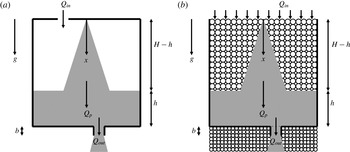
Schematic of emptying filling boxes devoid of (a) and filled with (b) porous media. Each box contains a single negatively buoyant plume, which is supposed to originate from either a point or a line source.

An equally recent theoretical and experimental development has been that of so-called porous media filling box flows in which case we imagine not a free turbulent plume but rather one that falls at low Reynolds number through a (uniform, isotropic) porous medium. In this vein, both closed (Sahu & Flynn Reference Sahu and Flynn2015, Reference Sahu and Flynn2016) and ventilated (Roes, Bolster & Flynn Reference Roes, Bolster and Flynn2014) control volumes have been examined. Problems of this sort are of particular interest in hydrology and related disciplines, as related e.g. to the (i) dissolution of non-aqueous phase liquids or geologically sequestered CO2 into potable groundwater (Neufeld et al. Reference Neufeld, Vella, Huppert and Lister2011; MacMinn et al. Reference MacMinn, Neufeld, Hesse and Huppert2012), (ii) leakage of contaminants from waste piles (Oostrom et al. Reference Oostrom, Rockhold, Thorne, Truex, Last and Rohay2007; Carroll et al. Reference Carroll, Oostrom, Truex, Rohay and Brusseau2012) and (iii) development and commercialization of enhanced oil recovery technologies such as cyclic steam stimulation and steam-assisted gravity drainage (Xu Reference Xu2008; Chen et al. Reference Chen, Liu, Elsworth, Connell and Pan2009).
Further to the above body of literature, a major objective of this study is to investigate time-dependent flows in an emptying filling box filled with a porous medium. For
 $t>0$
in which
 $t$
is time, the box is comprised of two fluid layers, an upper uncontaminated layer containing ambient fluid and a lower layer comprised of discharged plume fluid. (The plume fluid and ambient are assumed to be fully miscible one within the other.) The latter layer is continuously stratified, but approaches a uniform density in the long-time limit. Although the density profile in the contaminated layer for the case of a free turbulent plume can be obtained by adapting the numerical technique of Germeles (Reference Germeles1975), an analogue description specific to porous media plumes has not yet been developed. Even in the absence of such a model, however, meaningful bounds on the range of possible solutions can be obtained provided
 $t$
is not too small. Our approach is substantiated by drawing extensive comparisons with the analogue free turbulent plume flow. In this way, we identify the qualitative and quantitative similarities between these two categories of filling box model, one thoroughly studied over the past two decades, the other very much less so.
The rest of the discussion is organized as follows: in § 2, we formulate the problem with reference to boxes that are either filled with or devoid of porous media. Solutions derived assuming an initially uncontaminated box are then presented and discussed in § 3. In § 4, the criteria for the contaminated layer to overshoot its steady-state depth is outlined. Time-varying sources are then considered in §§ 5 and 6. We conclude with a detailed comparison between the free turbulent and porous media plume cases in § 7 and a series of summary remarks appropriate to the work as a whole in § 8.
2 Theory – basic formulation
We begin by investigating the flow dynamics of a ventilated filling box that is either filled with, or devoid of, a porous medium. A pair of schematics illustrating these two cases are presented in figure 1, which indicates the position of the negatively buoyant plumes relative to the lower openings. (In the porous media flow literature, such an opening is more typically referred to as a ‘fissure’. Likewise, in the natural ventilation literature, the term ‘vent’ is often applied. Because a major focus of this study is to draw a comparison between the porous media and free turbulent plume cases, we prefer to use the more generic term ‘opening’ throughout. We do so on the understanding that viscous dissipation respectively is and is not dynamically significant in the porous media and free turbulent flow scenarios.) These openings, along with the upper opening of figure 1(a) and the open top of figure 1(b), connect the box interior to an infinite external ambient of density
 $\unicode[STIX]{x1D70C}_{a}$
. Note that the difference of opening configuration along the upper boundary reflects the fact that porous media flows in nature, such as those mentioned in the previous section, are, in general, more realistically represented by an open upper boundary.
Applying conservation of volume and buoyancy to the lower contaminated layer leads to
 $$\begin{eqnarray}\displaystyle & \displaystyle \frac{\text{d}V}{\text{d}t}=Q_{p}-Q_{out}, & \displaystyle\end{eqnarray}$$
 $$\begin{eqnarray}\displaystyle & \displaystyle \frac{\text{d}(SI)}{\text{d}t}=F_{0}-Q_{out}g^{\prime }|_{x=H}, & \displaystyle\end{eqnarray}$$
where
 $V$
is the volume of the contaminated layer. In the case of a box devoid of porous media,
 $V=Sh$
where
 $S$
and
 $h$
denote the cross-sectional area of the box (independent of depth) and the depth of the lower contaminated layer, respectively. By contrast, if the box is filled with a porous medium,
 $V=\unicode[STIX]{x1D719}Sh$
in which
 $\unicode[STIX]{x1D719}$
is the porosity or void fraction. Meanwhile,
 $Q_{p}$
and
 $Q_{out}$
denote, respectively, the plume volume flux at the level of the interface and the volumetric rate of outflow through the lower opening.
 $F_{0}$
is the source buoyancy flux and
 $I$
is the integrated buoyancy of the contaminated layer, defined as
 $$\begin{eqnarray}I=\int _{H-h}^{H}g^{\prime }\,\text{d}x,\end{eqnarray}$$
in which
 $H$
is the total depth of the box and
 $g^{\prime }$
is the reduced gravity of the contaminated layer, i.e.
 $$\begin{eqnarray}g^{\prime }=g\frac{\unicode[STIX]{x1D70C}-\unicode[STIX]{x1D70C}_{a}}{\unicode[STIX]{x1D70C}_{a}}.\end{eqnarray}$$
Here
 $\unicode[STIX]{x1D70C}$
is the density of the contaminated layer, which we allow to vary in time,
 $t$
, and in the vertical direction. We assume a Boussinesq flow so that density differences are dynamically important only when they multiply gravitational acceleration.
In order to solve (2.1) and (2.2), we require expressions for
 $Q_{p}$
and
 $Q_{out}$
. These are given as follows (see for instance Kaye & Hunt Reference Kaye and Hunt2004; Roes et al.
Reference Roes, Bolster and Flynn2014):
 $$\begin{eqnarray}\displaystyle \text{free turbulent plume:}~Q_{p}=C_{j}F_{0}^{1/3}(x+x_{0})^{j},\quad Q_{out}=A^{\star }\sqrt{I+g^{\prime }|_{x=H}b},\qquad & & \displaystyle\end{eqnarray}$$
 $$\begin{eqnarray}\displaystyle \text{point-source porous media plume:}~Q_{p}=8\unicode[STIX]{x03C0}D\unicode[STIX]{x1D719}(x+x_{0}),\quad Q_{out}=\frac{Ak_{f}}{\unicode[STIX]{x1D708}b}(I+g^{\prime }|_{x=H}b), & & \displaystyle \nonumber\\ \displaystyle & & \displaystyle\end{eqnarray}$$
 $$\begin{eqnarray}\displaystyle \left.\begin{array}{@{}c@{}}\displaystyle \text{line-source porous media plume:}~Q_{p}=\left(\frac{36D\unicode[STIX]{x1D719}F_{0}k(x+x_{0})\unicode[STIX]{x1D6EC}^{2}}{\unicode[STIX]{x1D708}}\right)^{1/3},\\ \displaystyle Q_{out}=\frac{Ak_{f}}{\unicode[STIX]{x1D708}b}(I+g^{\prime }|_{x=H}b).\end{array}\right\}\qquad & & \displaystyle\end{eqnarray}$$
In (2.5)
 $j$
depends on the plume geometry, i.e.
 $j=5/3$
and
 $j=1$
correspond to point- and line-source plumes, respectively. Furthermore, the constant
 $C_{j}$
is obtained from the entrainment coefficient and source geometry,
 $x$
is the vertical coordinate measured relative to the source,
 $x_{0}$
is the virtual origin correction for non-ideal plumes having a finite source volume flux,
 $A^{\star }$
is the weighted area of the lower and upper openings and
 $b$
is the depth of the lower opening. In (2.6) and (2.7),
 $D$
denotes the solute dispersion coefficient which we assume to be spatially invariant (Wooding Reference Wooding1963). The problem of a spatially variable
 $D$
has been studied, among many others, by Sahu & Flynn (Reference Sahu and Flynn2015, Reference Sahu and Flynn2016) whose expressions for
 $Q_{p}$
could just as easily be used instead of the above formulas. Moreover,
 $A$
and
 $k_{f}$
denote, respectively, the cross-sectional area and permeability of the lower opening,
 $\unicode[STIX]{x1D708}$
is the kinematic viscosity,
 $k$
denotes the permeability of the box, and
 $\unicode[STIX]{x1D6EC}$
is the depth of the line source into the page. The virtual origin corrections in (2.5)–(2.7) are respectively defined as
 $$\begin{eqnarray}\displaystyle & \displaystyle \text{free turbulent plume:}~x_{0}=\left(\frac{Q_{0}}{C_{j}F_{0}^{1/3}}\right)^{1/j}, & \displaystyle\end{eqnarray}$$
 $$\begin{eqnarray}\displaystyle & \displaystyle \text{point-source porous media plume:}~x_{0}=\frac{Q_{0}}{8\unicode[STIX]{x03C0}D\unicode[STIX]{x1D719}}, & \displaystyle\end{eqnarray}$$
 $$\begin{eqnarray}\displaystyle & \displaystyle \text{line-source porous media plume:}~x_{0}=\frac{Q_{0}^{3}\unicode[STIX]{x1D708}}{36D\unicode[STIX]{x1D719}F_{0}k\unicode[STIX]{x1D6EC}^{2}}, & \displaystyle\end{eqnarray}$$
where
 $Q_{0}\,({>}0)$
is the plume source volume flux.
We define the average reduced gravity of the contaminated layer as
 $\bar{g}^{\prime }=I/h$
and use (2.5)–(2.7) to rewrite (2.1) and (2.2) as
 $$\begin{eqnarray}\displaystyle & \displaystyle S\frac{\text{d}h}{\text{d}t}=C_{j}F_{0}^{1/3}(H-h+x_{0})^{j}-A^{\star }\sqrt{\bar{g}^{\prime }h+g^{\prime }|_{x=H}b}, & \displaystyle\end{eqnarray}$$
 $$\begin{eqnarray}\displaystyle & \displaystyle S\frac{\text{d}(\bar{g}^{\prime }h)}{\text{d}t}=F_{0}-A^{\star }\sqrt{\bar{g}^{\prime }h+g^{\prime }|_{x=H}b}g^{\prime }|_{x=H}, & \displaystyle\end{eqnarray}$$
for a free turbulent plume, and as
 $$\begin{eqnarray}\displaystyle & \displaystyle \unicode[STIX]{x1D719}S\frac{\text{d}h}{\text{d}t}=8\unicode[STIX]{x03C0}D\unicode[STIX]{x1D719}(H-h+x_{0})-\frac{Ak_{f}}{\unicode[STIX]{x1D708}b}(\bar{g}^{\prime }h+g^{\prime }|_{x=H}b), & \displaystyle\end{eqnarray}$$
 $$\begin{eqnarray}\displaystyle & \displaystyle \unicode[STIX]{x1D719}S\frac{\text{d}(\bar{g}^{\prime }h)}{\text{d}t}=F_{0}-\frac{Ak_{f}}{\unicode[STIX]{x1D708}b}(\bar{g}^{\prime }h+g^{\prime }|_{x=H}b)g^{\prime }|_{x=H}, & \displaystyle\end{eqnarray}$$
for a point-source porous media plume and finally as
 $$\begin{eqnarray}\displaystyle & \displaystyle \unicode[STIX]{x1D719}S\frac{\text{d}h}{\text{d}t}=\left(\frac{36D\unicode[STIX]{x1D719}F_{0}k\unicode[STIX]{x1D6EC}^{2}}{\unicode[STIX]{x1D708}}\right)^{1/3}(H-h+x_{0})^{1/3}-\frac{Ak_{f}}{\unicode[STIX]{x1D708}b}(\bar{g}^{\prime }h+g^{\prime }|_{x=H}b), & \displaystyle\end{eqnarray}$$
 $$\begin{eqnarray}\displaystyle & \displaystyle \unicode[STIX]{x1D719}S\frac{\text{d}(\bar{g}^{\prime }h)}{\text{d}t}=F_{0}-\frac{Ak_{f}}{\unicode[STIX]{x1D708}b}(\bar{g}^{\prime }h+g^{\prime }|_{x=H}b)g^{\prime }|_{x=H}, & \displaystyle\end{eqnarray}$$
for a line-source porous media plume. We also introduce the following dimensionless parameters
 $$\begin{eqnarray}\unicode[STIX]{x1D709}=\frac{h}{H}\quad \text{and}\quad \left|\begin{array}{@{}ll@{}}\displaystyle \unicode[STIX]{x1D6FF}=\bar{g}^{\prime }\frac{C_{j}H^{j}}{F_{0}^{2/3}} & \text{(free turbulent plume)}\\ \displaystyle \unicode[STIX]{x1D6FF}=\bar{g}^{\prime }\frac{8\unicode[STIX]{x03C0}D\unicode[STIX]{x1D719}H}{F_{0}} & \text{(point-source porous media plume)}\\ \displaystyle \unicode[STIX]{x1D6FF}=\bar{g}^{\prime }\left(\frac{36D\unicode[STIX]{x1D719}kH\unicode[STIX]{x1D6EC}^{2}}{F_{0}^{2}\unicode[STIX]{x1D708}}\right)^{1/3} & \text{(line-source porous media plume)},\end{array}\right.\end{eqnarray}$$
where
 $\unicode[STIX]{x1D709}$
and
 $\unicode[STIX]{x1D6FF}$
represent a dimensionless interface depth and a dimensionless average reduced gravity of the contaminated layer, respectively. For an emptying filling box problem, two time scales are typically considered (Kaye & Hunt Reference Kaye and Hunt2004)
 $$\begin{eqnarray}\displaystyle & \displaystyle \text{free turbulent plume:}~T_{d}=\frac{SC_{j}^{1/2}H^{(j+1)/2}}{A^{\star }F_{0}^{1/3}},\quad T_{f}=\frac{S}{C_{j}F_{0}^{1/3}H^{(j-1)}},\qquad & \displaystyle\end{eqnarray}$$
 $$\begin{eqnarray}\displaystyle & \displaystyle \text{point-source porous media plume:}~T_{d}=\frac{8\unicode[STIX]{x03C0}D\unicode[STIX]{x1D719}^{2}\unicode[STIX]{x1D708}SH^{2}}{Ak_{f}F_{0}},\quad T_{f}=\frac{S}{8\unicode[STIX]{x03C0}D},\qquad & \displaystyle\end{eqnarray}$$
 $$\begin{eqnarray}\displaystyle & \displaystyle \left.\begin{array}{@{}c@{}}\displaystyle \text{line-source porous media plume:}~T_{d}=\left(\frac{36D\unicode[STIX]{x1D719}^{4}\unicode[STIX]{x1D708}^{2}k\unicode[STIX]{x1D6EC}^{2}S^{3}H^{4}}{A^{3}k_{f}^{3}F_{0}^{2}}\right)^{1/3},\\ \displaystyle T_{f}=\left(\frac{S^{3}\unicode[STIX]{x1D719}^{2}H^{2}\unicode[STIX]{x1D708}}{36DF_{0}k\unicode[STIX]{x1D6EC}^{2}}\right)^{1/3},\end{array}\right\}\qquad & \displaystyle\end{eqnarray}$$
where
 $T_{d}$
is the draining time scale and is proportional to the time taken for a contaminated layer spanning the entire depth of the box to drain completely through the lower opening. Meanwhile,
 $T_{f}$
is the filling time scale assuming an ideal plume with source buoyancy flux
 $F_{0}$
.
Having introduced the draining and filling time scales, we can now non-dimensionalize time according to
 $t=\sqrt{T_{d}T_{f}}\unicode[STIX]{x1D70F}$
. Equations (2.11) and (2.12) may then be rewritten for a free turbulent plume as
 $$\begin{eqnarray}\displaystyle & \displaystyle \frac{\text{d}\unicode[STIX]{x1D709}}{\text{d}\unicode[STIX]{x1D70F}}=\sqrt{\unicode[STIX]{x1D707}}\left(1-\unicode[STIX]{x1D709}+\frac{x_{0}}{H}\right)^{j}-\frac{1}{\sqrt{\unicode[STIX]{x1D707}}}\sqrt{\unicode[STIX]{x1D6FF}\unicode[STIX]{x1D709}+\unicode[STIX]{x1D6FF}|_{x=H}\frac{b}{H}}, & \displaystyle\end{eqnarray}$$
 $$\begin{eqnarray}\displaystyle & \displaystyle \frac{\text{d}\unicode[STIX]{x1D6FF}}{\text{d}\unicode[STIX]{x1D70F}}=\frac{\sqrt{\unicode[STIX]{x1D707}}}{\unicode[STIX]{x1D709}}\left[1-\unicode[STIX]{x1D6FF}\left(1-\unicode[STIX]{x1D709}+\frac{x_{0}}{H}\right)^{j}\right]+\frac{\unicode[STIX]{x1D6FF}-\unicode[STIX]{x1D6FF}|_{x=H}}{\sqrt{\unicode[STIX]{x1D707}}\unicode[STIX]{x1D709}}\sqrt{\unicode[STIX]{x1D6FF}\unicode[STIX]{x1D709}+\unicode[STIX]{x1D6FF}|_{x=H}\frac{b}{H}}. & \displaystyle\end{eqnarray}$$
The analogue, and similar looking, expressions for a laminar plume falling through a porous medium are given by
 $$\begin{eqnarray}\displaystyle & \displaystyle \frac{\text{d}\unicode[STIX]{x1D709}}{\text{d}\unicode[STIX]{x1D70F}}=\sqrt{\unicode[STIX]{x1D707}}\left(1-\unicode[STIX]{x1D709}+\frac{x_{0}}{H}\right)^{k}-\frac{1}{\sqrt{\unicode[STIX]{x1D707}}b/H}\left(\unicode[STIX]{x1D6FF}\unicode[STIX]{x1D709}+\unicode[STIX]{x1D6FF}|_{x=H}\frac{b}{H}\right), & \displaystyle\end{eqnarray}$$
 $$\begin{eqnarray}\displaystyle & \displaystyle \frac{\text{d}\unicode[STIX]{x1D6FF}}{\text{d}\unicode[STIX]{x1D70F}}=\frac{\sqrt{\unicode[STIX]{x1D707}}}{\unicode[STIX]{x1D709}}\left[1-\unicode[STIX]{x1D6FF}\left(1-\unicode[STIX]{x1D709}+\frac{x_{0}}{H}\right)^{k}\right]+\frac{\unicode[STIX]{x1D6FF}-\unicode[STIX]{x1D6FF}|_{x=H}}{\sqrt{\unicode[STIX]{x1D707}}\unicode[STIX]{x1D709}b/H}\left(\unicode[STIX]{x1D6FF}\unicode[STIX]{x1D709}+\unicode[STIX]{x1D6FF}|_{x=H}\frac{b}{H}\right), & \displaystyle\end{eqnarray}$$
where
 $k=1$
and
 $k=1/3$
correspond to point- and line-source plumes, respectively. In (2.21)–(2.24),
 $\unicode[STIX]{x1D707}$
is the ratio of the draining to the filling time scales. More explicitly,
 $$\begin{eqnarray}\displaystyle & \displaystyle \text{free turbulent plume:}~\unicode[STIX]{x1D707}=\frac{C_{j}^{3/2}H^{(3j-1)/2}}{A^{\star }}, & \displaystyle\end{eqnarray}$$
 $$\begin{eqnarray}\displaystyle & \displaystyle \text{point-source porous media plume:}~\unicode[STIX]{x1D707}=\frac{(8\unicode[STIX]{x03C0}D\unicode[STIX]{x1D719})^{2}\unicode[STIX]{x1D708}H^{2}}{Ak_{f}F_{0}}, & \displaystyle\end{eqnarray}$$
 $$\begin{eqnarray}\displaystyle & \displaystyle \text{line-source porous media plume:}~\unicode[STIX]{x1D707}=\left[\frac{(36D\unicode[STIX]{x1D719})^{2}\unicode[STIX]{x1D708}k^{2}\unicode[STIX]{x1D6EC}^{4}H^{2}}{A^{3}k_{f}^{3}F_{0}}\right]^{1/3}. & \displaystyle\end{eqnarray}$$
There arise two circumstances where the latter terms on the right-hand sides of (2.22) and (2.24) can be neglected. As noted by Bolster et al. (Reference Bolster, Maillard and Linden2008), who studied free turbulent plumes, the ratio of the latter to the former terms on the right-hand sides of (2.22) and (2.24) are proportional to
 $\unicode[STIX]{x1D707}$
. Hence, for large
 $\unicode[STIX]{x1D707}$
, these latter terms, which specifically incorporate the stratification of the contaminated layer, become negligible compared to the former terms. The latter terms can also be ignored assuming a well-mixed model. In this case, the density of the contaminated layer is assumed to be spatially uniform such that there is no difference between
 $\unicode[STIX]{x1D6FF}$
and
 $\unicode[STIX]{x1D6FF}|_{x=H}$
.
Far from being an abstract idealization, the well-mixed solution is, in fact, always approached in the long-time limit as a result of the continuous re-entrainment of contaminated fluid into the plume and its subsequent discharge along the bottom of the box. From (2.21)–(2.24) it is elementary to determine the steady-state depth,
 $\unicode[STIX]{x1D709}_{ss}$
, and reduced gravity,
 $\unicode[STIX]{x1D6FF}_{ss}$
, of the contaminated layer either by solving
 $$\begin{eqnarray}\displaystyle & \displaystyle \unicode[STIX]{x1D707}^{2}\left(1-\unicode[STIX]{x1D709}_{ss}+\frac{x_{0}}{H}\right)^{3j}=\left(\unicode[STIX]{x1D709}_{ss}+\frac{b}{H}\right), & \displaystyle\end{eqnarray}$$
 $$\begin{eqnarray}\displaystyle & \displaystyle \unicode[STIX]{x1D6FF}_{ss}=\frac{1}{\left(1-\unicode[STIX]{x1D709}_{ss}+{\displaystyle \frac{x_{0}}{H}}\right)^{j}}, & \displaystyle\end{eqnarray}$$
for a free turbulent plume, or
 $$\begin{eqnarray}\displaystyle & \displaystyle \unicode[STIX]{x1D707}\left(1-\unicode[STIX]{x1D709}_{ss}+\frac{x_{0}}{H}\right)^{2k}\left(\frac{b}{H}\right)=\left(\unicode[STIX]{x1D709}_{ss}+\frac{b}{H}\right), & \displaystyle\end{eqnarray}$$
 $$\begin{eqnarray}\displaystyle & \displaystyle \unicode[STIX]{x1D6FF}_{ss}=\frac{1}{\left(1-\unicode[STIX]{x1D709}_{ss}+{\displaystyle \frac{x_{0}}{H}}\right)^{k}}, & \displaystyle\end{eqnarray}$$
for a porous media plume. Furthermore, from (2.28) and (2.30) we can determine the range of
 $\unicode[STIX]{x1D707}$
for which
 $\unicode[STIX]{x1D709}$
assumes a physical value of between 0 and 1, to wit
 $$\begin{eqnarray}\displaystyle & \displaystyle \text{free turbulent plume:}~\frac{\sqrt{b/H}}{\sqrt{(1+x_{0}/H)^{3j}}}<\unicode[STIX]{x1D707}<\frac{\sqrt{1+b/H}}{(x_{0}/H)^{3j}}, & \displaystyle\end{eqnarray}$$
 $$\begin{eqnarray}\displaystyle & \displaystyle \text{porous media plume:}~\frac{1}{(1+x_{0}/H)^{2k}}<\unicode[STIX]{x1D707}<\frac{1+b/H}{(b/H)(x_{0}/H)^{2k}}. & \displaystyle\end{eqnarray}$$
For
 $\unicode[STIX]{x1D707}$
smaller than the lower bound, the draining capacity of the box is much larger than the filling capacity of the source so that a contaminated layer is never realized. On the other hand, for
 $\unicode[STIX]{x1D707}$
larger than the upper bound, the outflow from the lower opening cannot balance the source volume flux and contaminated fluid therefore occupies the entirety of the box; hence, a ventilation flow is not obtained.
In order to derive bounds on the range of possible solutions for the depth and reduced gravity of the contaminated layer, we examine two limiting cases. Firstly, we consider a scenario in which the lower layer is, in spite of the possible presence of stratification, assumed to be well mixed, i.e. the density is assumed to be spatially uniform within the contaminated layer for all
 $t$
rather than just large
 $t$
. Hence, the latter terms from the right-hand sides of (2.22) and (2.24) disappear. In the bookend opposite limiting case (hereafter referred to as the ‘approximate stratified model’), the density of the lower layer at the bottom of the box, which is unknown in the case of porous media plumes, is assumed equal to the plume density at the level of the interface. This plume density, which we express in terms of the reduced gravity as
 $g_{p}^{\prime }(x=H-h)=F_{0}/Q_{p}$
, is the largest possible density that can be achieved within the contaminated layer whether or not the interface is stationary. Accordingly the factor
 $\unicode[STIX]{x1D6FF}|_{x=H}$
that appears in (2.21)–(2.24) is replaced with
 $1/(1-\unicode[STIX]{x1D709}+x_{0}/H)^{j}$
for free turbulent plumes and
 $1/(1-\unicode[STIX]{x1D709}+x_{0}/H)^{k}$
for porous media plumes.
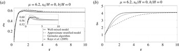
Evolution of the contaminated layer non-dimensional depth (a) and reduced gravity (b) calculated from Germeles (Reference Germeles1975), the well-mixed model given by (2.21) and (2.22) with spatially uniform
 $\unicode[STIX]{x1D6FF}$
and the approximate stratified model given by (2.21) and (2.22) with
 $\unicode[STIX]{x1D6FF}|_{x=H}$
specified using the plume density at the level of the ambient interface. Also included is the evolution of the contaminated layer depth as extracted from figure 12 of Kaye, Ji & Cook (Reference Kaye, Ji and Cook2009). Here we assume an ideal point-source free turbulent plume with
 $x_{0}/H=0$
; moreover,
 $b/H=0$
and
 $\unicode[STIX]{x1D707}=6.2$
.

So as to validate the legitimacy of the above approach, we apply the Germeles (Reference Germeles1975) numerical technique to the free turbulent plume problem (2.21)–(2.22) to confirm that Germeles’s ‘exact’ filling box solution is bounded by the above limiting cases, at least when
 $\unicode[STIX]{x1D70F}$
is not small. A comparison of model output is presented in figure 2, which shows the Germeles’s exact filling box, well-mixed and approximate stratified model solutions for canonical conditions, i.e.
 $\unicode[STIX]{x1D707}=6.2$
and
 $x_{0}/H=b/H=0$
. Also included in figure 2(a) are data corresponding to the numerical simulations of Kaye et al. (Reference Kaye, Ji and Cook2009), whose results were shown to agree very well with a series of small-scale laboratory experiments and theoretical models – see e.g. their figure 12. Shortly after ‘turning on’ the source, figure 2 indicates that the Germeles’s solution becomes bracketed by those of the well-mixed and approximate stratified models. The initial discrepancy is due to the fact that in our numerical solutions of (2.21) and (2.22) the non-dimensional reduced gravity of the contaminated layer can never start from a value less than unity, i.e. in the aforementioned limiting cases the initial conditions are given by
 $$\begin{eqnarray}\unicode[STIX]{x1D709}=0,\quad \text{and}\quad \unicode[STIX]{x1D6FF}=\frac{1}{\left(1+{\displaystyle \frac{x_{0}}{H}}\right)^{j}}\quad \text{at}~\unicode[STIX]{x1D70F}=0.\end{eqnarray}$$
By contrast, the initial conditions for the Germeles (Reference Germeles1975) algorithm assuming an ambient that is initially unstratified read
 $\unicode[STIX]{x1D709}=0$
and
 $\unicode[STIX]{x1D6FF}=0$
at
 $\unicode[STIX]{x1D70F}=0$
. Hence, it takes some finite, but generally small, time,
 $\unicode[STIX]{x1D70F}_{cr}$
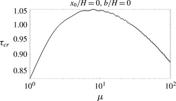
, for the system to evolve to the point that the Germeles’s solution becomes bracketed. Elaborating on this point, figure 3 shows
 $\unicode[STIX]{x1D70F}_{cr}$
for an ideal point-source plume with
 $b/H=0$
. Initially,
 $\unicode[STIX]{x1D70F}_{cr}$
increases with
 $\unicode[STIX]{x1D707}$
; the maximum
 $\unicode[STIX]{x1D70F}_{cr}$
corresponds to the maximum overshoot of contaminated layer depth, which is discussed in further detail below. As
 $\unicode[STIX]{x1D707}$
increases still further, the contaminated layer deepens comparatively rapidly; hence,
 $\unicode[STIX]{x1D70F}_{cr}$
decreases with
 $\unicode[STIX]{x1D707}$
. Note that, in the following sections where we study a cyclic or time-variable buoyancy source, the exact solution is bounded for all
 $\unicode[STIX]{x1D70F}$
when we start from a non-zero contaminated layer depth.
Non-dimensional time needed for the Germeles solution to become bracketed by the well-mixed and approximate stratified models. We consider here an ideal point-source plume with
 $b/H=0$
. Qualitatively similar results (not shown) are obtained for other plume configurations.

Of course, figure 2 presents results for a relatively classical problem, namely an emptying filling box for a box devoid of porous media, rather than the more novel problem of a laminar, porous media plume in a ventilated box. To reiterate, our motivation for revisiting such a classical problem is that it gives us good confidence that a similar approach of bounding the exact solution can be applied when considering porous media convection where, as already highlighted, no analogue to the Germeles (Reference Germeles1975) algorithm has ever been derived. Following on from the previous discussion, this confidence is based on the strong similarities between (2.21)–(2.22) and (2.23)–(2.24) which, in turn, follows from a judicious non-dimensionalization of the relevant governing equations. In summary, and although an exact solution is unavailable for the flow of figure 1(b), we expect such a solution to be bounded by the appropriate limiting cases of (2.23) and (2.24); the vertical distance between these bounds decreases substantially in the limit of large
 $\unicode[STIX]{x1D707}$
. Note finally that the bounds are little influenced by the effects of ambient diffusion/dispersion because (2.3) depends on the integral of the density difference rather than its vertical distribution. As an example, if one were to allow for some intermingling of contaminated and uncontaminated fluid parcels across the ambient interface (as has been done for filling boxes devoid of porous media by Baines Reference Baines1983 and Kaye et al.
Reference Kaye, Flynn, Cook and Ji2010), the outflux would not change. Thus the neglect of ambient diffusion/dispersion, which is formally valid for sufficiently large
 $Q_{p}\sqrt{t/D\unicode[STIX]{x1D719}}/S$
, is not a major limitation of the analysis to follow.
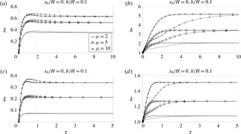
Ideal point-source free turbulent and porous media plumes with
 $\unicode[STIX]{x1D707}=\{2,5,10\}$
and
 $b/H=0.1$
. (a,b) Free turbulent plumes and (c,d) porous media plumes. The solid and dashed curves correspond to the well-mixed and approximate stratified models, respectively.

3 Initial transient
From figure 2 and the discussion thereof, we expect to be able to bracket exact solutions to (2.23) and (2.24) provided
 $\unicode[STIX]{x1D70F}$
is not too small. On this basis, we now proceed to solve these equations using the aforementioned assumptions so as to infer the true behaviour of porous media filling box flows. For the case where the initial interior density is the ambient density, we take
 $\unicode[STIX]{x1D70F}=0$
as the moment when the plume first touches the bottom of the box. Therefore, similar to (2.34), the initial conditions read
 $$\begin{eqnarray}\unicode[STIX]{x1D709}=0,\quad \text{and}\quad \unicode[STIX]{x1D6FF}=\frac{1}{\left(1+{\displaystyle \frac{x_{0}}{H}}\right)^{k}}\quad \text{at}~\unicode[STIX]{x1D70F}=0.\end{eqnarray}$$
Figure 4 shows the evolution of
 $\unicode[STIX]{x1D709}$
and
 $\unicode[STIX]{x1D6FF}$
for ideal point-source free turbulent and porous media plumes with
 $b/H=0.1$
. (Because the evolution of
 $\unicode[STIX]{x1D709}$
and
 $\unicode[STIX]{x1D6FF}$
in the line-source case is qualitatively similar to the behaviour seen in the point-source case, the former set of figures is not shown for the sake of brevity. In a similar spirit, and in §§ 5–7, whenever the results for point- and line-source plumes are qualitatively similar, only the figures for point-source plumes will be presented.) When
 $\unicode[STIX]{x1D707}$
is small, the contaminated layer is highly stratified. Dense fluid continuously drains from the bottom of the box and therefore the time rate of the increase of the average density of the contaminated layer is small compared to cases where
 $\unicode[STIX]{x1D707}$
is large and the contaminated layer has a more or less uniform density profile. Hence, the outflow volume flux, which depends on this average density, increases comparatively slowly and the contaminated layer thickens quickly. Consequently, the contaminated layer first reaches then exceeds its steady-state depth. Over time,
 $\unicode[STIX]{x1D709}$
relaxes back to this steady-state value as the filling and draining of the contaminated layer become balanced. On the other hand, when
 $\unicode[STIX]{x1D707}$
is large, there is, as noted before, relatively little vertical variation in the density of the contaminated layer. Now, however, the filling time scale is smaller than the draining time scale. Therefore, an overshoot of contaminated layer depth is again observed. We defer till § 7 a quantitative comparison of the maximum overshoots for small and large
 $\unicode[STIX]{x1D707}$
. Suffice it to say for now that (i) the overshoot is, in magnitude, comparable for the free turbulent and porous media plume cases, but, (ii) the steady-state depth of the contaminated layer is greater in the free turbulent plume case for the same
 $\unicode[STIX]{x1D707}$
(figure 4). This difference can be explained by comparing the latter terms from the right-hand sides of (2.21) and (2.23) which describe the outflow volume flux. Due to the difference in the exponents, and for fixed
 $\unicode[STIX]{x1D707}$
,
 $x_{0}/H$
and
 $b/H$
, the outflow volume flux is smaller for a box devoid of porous media. As a result, the steady-state depth and reduced gravity of the contaminated layer are both larger when the plume is of free turbulent type. Note finally that with the approximate stratified model, we can predict the overshoot in the contaminated layer depth for both small and large
 $\unicode[STIX]{x1D707}$
. In the case of the well-mixed model, by contrast, overshoot requires that a threshold value of
 $\unicode[STIX]{x1D707}$
is first exceeded – see Kaye & Hunt (Reference Kaye and Hunt2004) and the discussion of the next section.
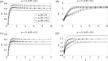
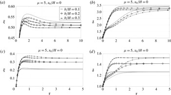
Figures 5 and 6 respectively show the effects of changing
 $x_{0}/H$
and
 $b/H$
on the evolution of the contaminated layer depth and reduced gravity. As confirmed by the former figure, increasing
 $x_{0}/H$
results in an increase in the contaminated layer depth and a decrease in its reduced gravity for both free turbulent and porous media plumes. Meanwhile increasing the depth of the opening increases the hydrostatic draining capacity of filling boxes devoid of porous media. This, in turn, results in a decrease in the contaminated layer depth and reduced gravity. However, in the case of a box filled with a porous medium, outflow is dominated by viscous drag and increasing the lower opening depth decreases, rather than increases,
 $Q_{out}$
– see (2.6) and (2.7). Thus, the contaminated layer depth and reduced gravity increase with
 $b/H$
.
Point-source free turbulent and porous media plumes with
 $\unicode[STIX]{x1D707}=5$
,
 $x_{0}/H=\{0,0.1,0.2\}$
and
 $b/H=0.1$
. (a,b) Free turbulent plumes and (c,d) porous media plumes. The solid and dashed curves correspond to the well-mixed and approximate stratified models, respectively.

Ideal point-source free turbulent and porous media plumes with
 $\unicode[STIX]{x1D707}=5$
and
 $b/H=\{0.1,0.2,0.3\}$
. (a,b) Free turbulent plumes and (c,d) porous media plumes. The solid and dashed curves correspond to the well-mixed and approximate stratified models, respectively.

4 Overshoot criteria
In order to compute, for the case of a well-mixed contaminated layer, the value of
 $\unicode[STIX]{x1D707}$
at which overshoot first occurs for given
 $x_{0}/H$
and
 $b/H$
, we linearize (2.21)–(2.22) and (2.23)–(2.24) about their steady-state values, i.e.
 $$\begin{eqnarray}\left[\begin{array}{@{}c@{}}\dot{\unicode[STIX]{x1D709}}\\ \dot{\unicode[STIX]{x1D6FF}}\end{array}\right]\approx \left[\begin{array}{@{}cc@{}}\left.{\displaystyle \frac{\unicode[STIX]{x2202}\dot{\unicode[STIX]{x1D709}}}{\unicode[STIX]{x2202}\unicode[STIX]{x1D709}}}\right|_{\unicode[STIX]{x1D6FF}=\unicode[STIX]{x1D6FF}_{ss},\unicode[STIX]{x1D709}=\unicode[STIX]{x1D709}_{ss}} & \left.{\displaystyle \frac{\unicode[STIX]{x2202}\dot{\unicode[STIX]{x1D709}}}{\unicode[STIX]{x2202}\unicode[STIX]{x1D6FF}}}\right|_{\unicode[STIX]{x1D6FF}=\unicode[STIX]{x1D6FF}_{ss},\unicode[STIX]{x1D709}=\unicode[STIX]{x1D709}_{ss}}\\ \left.{\displaystyle \frac{\unicode[STIX]{x2202}\dot{\unicode[STIX]{x1D6FF}}}{\unicode[STIX]{x2202}\unicode[STIX]{x1D709}}}\right|_{\unicode[STIX]{x1D6FF}=\unicode[STIX]{x1D6FF}_{ss},\unicode[STIX]{x1D709}=\unicode[STIX]{x1D709}_{ss}} & \left.{\displaystyle \frac{\unicode[STIX]{x2202}\dot{\unicode[STIX]{x1D6FF}}}{\unicode[STIX]{x2202}\unicode[STIX]{x1D6FF}}}\right|_{\unicode[STIX]{x1D6FF}=\unicode[STIX]{x1D6FF}_{ss},\unicode[STIX]{x1D709}=\unicode[STIX]{x1D709}_{ss}}\end{array}\right]\left[\begin{array}{@{}c@{}}\unicode[STIX]{x1D709}-\unicode[STIX]{x1D709}_{ss}\\ \unicode[STIX]{x1D6FF}-\unicode[STIX]{x1D6FF}ss\end{array}\right].\end{eqnarray}$$
Following Kaye & Hunt (Reference Kaye and Hunt2004), we draw an analogy with a mass–spring–damper system, i.e. the system is overdamped when the above matrix has two distinct real eigenvalues and is underdamped when the eigenvalues are complex conjugates. For given
 $x_{0}/H$
and
 $b/H$
, we numerically determine
 $\unicode[STIX]{x1D707}_{c}$
, the critical value of
 $\unicode[STIX]{x1D707}$
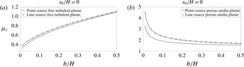
, corresponding to the boundary between an over- and underdamped system. Figure 7 shows
 $\unicode[STIX]{x1D707}_{c}$
for ideal free turbulent and porous media plumes as functions of
 $b/H$
.
 $\unicode[STIX]{x1D707}_{c}$
for ideal free turbulent and porous media plumes as a function of
 $b/H$
. (a) Free turbulent plumes and (b) porous media plumes.

To reiterate, in the case of a box devoid of porous media, increasing the depth of the lower opening results in an increase in the hydrostatic pressure difference between inside and outside, which, in turn, increases the outflow of contaminated fluid. Thus, for the contaminated layer to overshoot, the filling capacity of the box should likewise increase to compensate, i.e. the filling time scale should decrease. It is no surprise then that an increase in
 $b/H$
corresponds to an increase in
 $\unicode[STIX]{x1D707}_{c}$
in figure 7(a). When the box is filled with porous media, however, (2.6) and (2.7) indicate that the outflow volume flux is inversely proportional to the depth of the lower opening. Therefore, increasing
 $b/H$
in figure 7(b) results in a decrease in
 $\unicode[STIX]{x1D707}_{c}$
.
Although the overshoot criterion discussed in this section is clearly related to the transient evolution of the system, it must be reiterated that the source is assumed time independent for all cases considered thus far. There are, however, numerous scenarios where a time-variable source constitutes a more reasonable approximation. For instance, and for a filling box devoid of porous media, we imagine a naturally ventilated lecture theatre that is occupied intermittently throughout the day. Conversely, and in the case of a porous media filling box, technologies such as cyclic steam stimulation or CO2 ‘huff ’n puff’ both entail periodic fluid injections for purposes of enhanced oil recovery. Motivated by these and other examples, we turn in the next two sections to a discussion of time-variable source conditions.
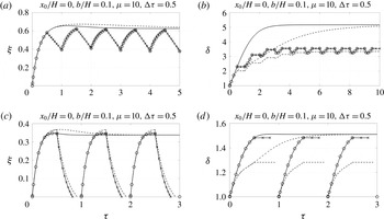
Ideal free turbulent and porous media plume responses to cyclic variations in the source conditions with
 $b/H=0.1$
,
 $\unicode[STIX]{x1D707}=10$
and
 $\unicode[STIX]{x0394}\unicode[STIX]{x1D70F}=0.25$
. (a,b) Free turbulent plume and (c,d) porous media plume. The thick solid curves pertain to the well-mixed case where the source remains on indefinitely. The curves with circle and cross markers correspond to the time periods when the source is respectively on and off. Similar comments apply to the dashed curves, though these correspond to the approximate stratified model.

5 Transient source turned on and off
Consider now a situation where the plume source is sequentially turned on and off with a half-period of
 $\unicode[STIX]{x0394}\unicode[STIX]{x1D70F}$
. When the plume source is off, contaminated fluid continues to be discharged from the bottom of the box. As a consequence, the lower layer depth decreases monotonically in time until the source is again turned on. If the contaminated layer drains completely, i.e. if
 $\unicode[STIX]{x0394}\unicode[STIX]{x1D70F}$
is sufficiently large, the box then consists of uniform ambient fluid just as with the presumed initial condition. For
 $\unicode[STIX]{x0394}\unicode[STIX]{x1D70F}$
less than this critical value, the contaminated layer remains of finite thickness; its reduced gravity equals the value at the instant the source was turned off.
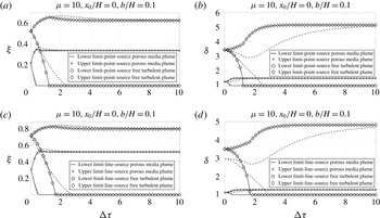
Figure 8 shows the evolution of
 $\unicode[STIX]{x1D709}$
and
 $\unicode[STIX]{x1D6FF}$
for ideal point-source free turbulent and porous media plumes with
 $\unicode[STIX]{x1D707}=10$
,
 $b/H=0.1$
, and
 $\unicode[STIX]{x0394}\unicode[STIX]{x1D70F}=0.25$
. If
 $\unicode[STIX]{x0394}\unicode[STIX]{x1D70F}$
is smaller than the non-dimensional time required for the system to approach steady state,
 $\unicode[STIX]{x1D709}_{ss}$
and
 $\unicode[STIX]{x1D6FF}_{ss}$
will never be realized regardless of the number of cycles. Rather, after a few cycles, the depth of the lower layer oscillates between two extrema whose values depend on the magnitude of
 $\unicode[STIX]{x0394}\unicode[STIX]{x1D70F}$
in addition to
 $\unicode[STIX]{x1D707}$
,
 $x_{0}/H$
and
 $b/H$
(figure 8
a,b). Consistent with the discussion of the previous paragraph and for sufficiently large
 $\unicode[STIX]{x0394}\unicode[STIX]{x1D70F}$
, the lower extrema corresponds to a box devoid of contaminated fluid (figure 8
c,d). Also, consistent with our previous discussions, the time rate of increase of the contaminated layer depth is greater for the approximate stratified model compared to the well-mixed model. Hence, for the period when the source is on, the contaminated layer reaches a greater depth and correspondingly it takes longer for the contaminated fluid to drain out of the box for the period when the source is off.
6 Transient source turned up or down
Building on the material of the previous section, we now consider a limited increase or decrease in the source buoyancy flux or volume flux. Thus the source buoyancy flux might change from an initial value of
 $F_{0}$
to
 $F_{0}+\unicode[STIX]{x0394}F$
or the source volume flux might change from an initial value of
 $Q_{0}$
to
 $Q_{0}+\unicode[STIX]{x0394}Q$
. Note that
 $\unicode[STIX]{x0394}F$
and
 $\unicode[STIX]{x0394}Q$
can be either positive or negative quantities but, by assumption,
 $F_{0}+\unicode[STIX]{x0394}F>0$
and
 $Q_{0}+\unicode[STIX]{x0394}Q>0$
. Note also that a change in
 $Q$
is not supposed to result in a change in
 $F$
and vice versa, i.e.
 $\unicode[STIX]{x0394}Q$
and
 $\unicode[STIX]{x0394}F$
are assumed to be uncorrelated.
Given a final buoyancy flux
 $F_{0}+\unicode[STIX]{x0394}F$
or a volume flux
 $Q_{0}+\unicode[STIX]{x0394}Q$
, we can rewrite (2.21)–(2.24) as
 $$\begin{eqnarray}\displaystyle & \displaystyle \frac{\text{d}\unicode[STIX]{x1D709}}{\text{d}\unicode[STIX]{x1D70F}}=\unicode[STIX]{x1D712}_{1}^{1/3}\sqrt{\unicode[STIX]{x1D707}}\left[1-\unicode[STIX]{x1D709}+\left(\frac{\unicode[STIX]{x1D712}_{2}}{\unicode[STIX]{x1D712}_{1}^{1/3}}\right)^{1/j}\frac{x_{0}}{H}\right]^{j}-\frac{1}{\sqrt{\unicode[STIX]{x1D707}}}\sqrt{\unicode[STIX]{x1D6FF}\unicode[STIX]{x1D709}+\unicode[STIX]{x1D6FF}|_{x=H}\frac{b}{H}}, & \displaystyle\end{eqnarray}$$
 $$\begin{eqnarray}\displaystyle & \displaystyle \frac{\text{d}\unicode[STIX]{x1D6FF}}{\text{d}\unicode[STIX]{x1D70F}}=\frac{\sqrt{\unicode[STIX]{x1D707}}}{\unicode[STIX]{x1D709}}\left\{\unicode[STIX]{x1D712}_{1}-\unicode[STIX]{x1D712}_{1}^{1/3}\unicode[STIX]{x1D6FF}\left[1-\unicode[STIX]{x1D709}+\left(\frac{\unicode[STIX]{x1D712}_{2}}{\unicode[STIX]{x1D712}_{1}^{1/3}}\right)^{1/j}\frac{x_{0}}{H}\right]^{j}\right\}+\frac{\unicode[STIX]{x1D6FF}-\unicode[STIX]{x1D6FF}|_{x=H}}{\sqrt{\unicode[STIX]{x1D707}}}\sqrt{\frac{\unicode[STIX]{x1D6FF}\unicode[STIX]{x1D709}+\unicode[STIX]{x1D6FF}|_{x=H}b/H}{\unicode[STIX]{x1D709}^{2}}}, & \displaystyle \nonumber\\ \displaystyle & & \displaystyle\end{eqnarray}$$
for a free turbulent plume and
 $$\begin{eqnarray}\displaystyle & \displaystyle \frac{\text{d}\unicode[STIX]{x1D709}}{\text{d}\unicode[STIX]{x1D70F}}=\unicode[STIX]{x1D712}_{1}^{n}\sqrt{\unicode[STIX]{x1D707}}\left[1-\unicode[STIX]{x1D709}+\left(\frac{\unicode[STIX]{x1D712}_{2}}{\unicode[STIX]{x1D712}_{1}^{n}}\right)^{1/k}\frac{x_{0}}{H}\right]^{k}-\frac{1}{\sqrt{\unicode[STIX]{x1D707}}b/H}\left(\unicode[STIX]{x1D6FF}\unicode[STIX]{x1D709}+\unicode[STIX]{x1D6FF}|_{x=H}\frac{b}{H}\right), & \displaystyle\end{eqnarray}$$
 $$\begin{eqnarray}\displaystyle & \displaystyle \frac{\text{d}\unicode[STIX]{x1D6FF}}{\text{d}\unicode[STIX]{x1D70F}}=\frac{\sqrt{\unicode[STIX]{x1D707}}}{\unicode[STIX]{x1D709}}\left\{\unicode[STIX]{x1D712}_{1}-\unicode[STIX]{x1D712}_{1}^{n}\unicode[STIX]{x1D6FF}\left[1-\unicode[STIX]{x1D709}+\left(\frac{\unicode[STIX]{x1D712}_{2}}{\unicode[STIX]{x1D712}_{1}^{n}}\right)^{1/k}\frac{x_{0}}{H}\right]^{k}\right\}+\frac{\unicode[STIX]{x1D6FF}-\unicode[STIX]{x1D6FF}|_{x=H}}{\sqrt{\unicode[STIX]{x1D707}}b/H}\left(\frac{\unicode[STIX]{x1D6FF}\unicode[STIX]{x1D709}+\unicode[STIX]{x1D6FF}|_{x=H}b/H}{\unicode[STIX]{x1D709}}\right), & \displaystyle \nonumber\\ \displaystyle & & \displaystyle\end{eqnarray}$$
for a porous media plume where
 $$\begin{eqnarray}\unicode[STIX]{x1D712}_{1}=\frac{F_{0}+\unicode[STIX]{x0394}F}{F_{0}}\quad \text{and}\quad \unicode[STIX]{x1D712}_{2}=\frac{Q_{0}+\unicode[STIX]{x0394}Q}{Q_{0}}.\end{eqnarray}$$
Also, in (6.3) and (6.4),
 $n=0$
and
 $n=1/3$
correspond to point- and line-source porous media plumes, respectively.
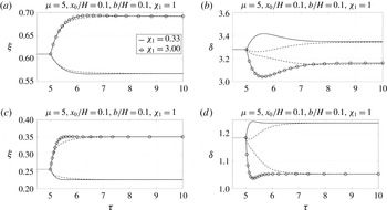
Figure 9 shows the effect of changing the source volume flux of point-source free turbulent and porous media plumes with
 $\unicode[STIX]{x1D707}=5$
,
 $x_{0}/H=0.1$
and
 $b/H=0.1$
. In both cases, the lower layer reduced gravity decreases (increases) for an increase (decrease) in the source volume flux. As a result, the outflow volume flux becomes smaller (larger) and the contaminated layer depth increases (decreases) to compensate. It should be emphasized that, for both categories of plume, the steady-state depth of the contaminated layer depends on the source volume flux. Therefore changing the source volume flux results in a permanent change in the steady-state value of
 $\unicode[STIX]{x1D709}$
(and, of course,
 $\unicode[STIX]{x1D6FF}$
).
Effects of changing the source volume flux of point-source free turbulent and porous media plumes with
 $\unicode[STIX]{x1D707}=10$
,
 $b/H=0.1$
and an initial value of
 $x_{0}/H$
given by 0.1. (a,b) Free turbulent plume and (c,d) porous media plume. The dotted curves show the initial evolution of the system toward steady state before changing the source volume flux at
 $\unicode[STIX]{x1D70F}=5$
. Also, the dashed curves show model predictions corresponding to the approximate stratified model.

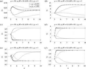
Figure 10 illustrates the effect of changing the source buoyancy flux of an ideal point-source free turbulent plume, and ideal point- and line-source porous media plumes with
 $\unicode[STIX]{x1D707}=10$
and
 $b/H=0.1$
. In the case of a free turbulent plume, an increase (decrease) in the source buoyancy flux results in a transient increase (decrease) in the depth of the contaminated layer. However, as the outflow from the contaminated layer adjusts, so too does
 $\unicode[STIX]{x1D709}$
; ultimately the interface depth returns to its previous value. Qualitatively different behaviour is seen for the case of porous media plumes. Unlike the free turbulent plume case where the steady-state depth of the contaminated layer is independent of the source buoyancy flux, the new value for
 $\unicode[STIX]{x1D709}_{ss}$
is now different from the value observed before adjusting
 $F_{0}$
. For the case of line-source porous media plumes, increasing (decreasing) the source buoyancy flux increases (decreases) the plume volume flux. Thus, the depth of the contaminated layer initially rises (falls). Correspondingly, the outflow volume flux increases (decreases) and ultimately balances the plume volume flux at a new ambient interface elevation, which is lower (higher) than its original value. However, for the case of point-source porous media plumes, (2.6) shows that the plume volume flux is, surprisingly, independent of the source buoyancy flux. Therefore, an increase (decrease) in the source buoyancy flux does not result in an initial transient increase (decrease) in the contaminated layer depth. Rather, the variation of
 $\unicode[STIX]{x1D709}$
with
 $\unicode[STIX]{x1D70F}$
is monotonic as is confirmed by figure 10(c).
Effects of changing the source buoyancy flux of ideal point-source free turbulent, and ideal point- and line-source porous media plumes with
 $\unicode[STIX]{x1D707}=10$
and
 $b/H=0.1$
. (a,b) Free turbulent plume, (c,d) point-source porous media plume and (e,f) line-source porous media plume. The dotted curves show the initial evolution of the system toward steady-state values before changing the source buoyancy flux at
 $\unicode[STIX]{x1D70F}=5$
. Also, the dashed curves show model predictions corresponding to the approximate stratified model.

7 Comparison of point- and line-source plumes in boxes filled with and devoid of porous media
Up until now, our comparisons between porous media laminar and free turbulent plumes have not been especially direct. In figures 9 and 10, for instance, the two plume types are considered in separate panels. However, an objective of our study is to quantify points of similarity and difference between these flow scenarios. Therefore, in this penultimate section, we will more directly compare flow characteristics in emptying filling boxes filled with and devoid of porous media. Because changing
 $x_{0}/H$
and
 $b/H$
does not alter the dynamical features of the system except for an increase or a decrease in the contaminated layer depth and reduced gravity, this comparison shall mostly consider ideal plumes with fixed lower opening depth.
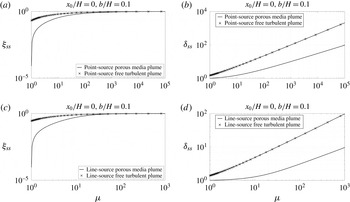
Figure 11 illustrates, for fixed
 $x_{0}/H$
and
 $b/H$
, the variation of the depth and reduced gravity of the contaminated layer as a function of
 $\unicode[STIX]{x1D707}$
. As expected, and for both types of plume,
 $\unicode[STIX]{x1D709}_{ss}$
increases from close to zero for small
 $\unicode[STIX]{x1D707}$
, to close to unity for large
 $\unicode[STIX]{x1D707}$
. Also, and for both plume geometries (i.e. point and line source), the contaminated layer depth and reduced gravity is greater in the case of a free turbulent plume versus a porous media plume.
 $\unicode[STIX]{x1D709}_{ss}$
and
 $\unicode[STIX]{x1D6FF}_{ss}$
as functions of
 $\unicode[STIX]{x1D707}$
for ideal free turbulent and porous media plumes with
 $b/H=0.1$
. (a,b) Point-source plumes and (c,d) line-source plumes.

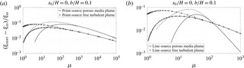
Figure 12 shows the magnitude of the overshoot relative to the steady-state depth. For small values of
 $\unicode[STIX]{x1D707}$
this relative magnitude is greater for free turbulent plumes which suggests a higher stratification in the contaminated layer. However, as
 $\unicode[STIX]{x1D707}$
increases, the relative magnitude of the overshoot becomes greater in the porous media plume case. Moreover, the relative magnitude of the overshoot is more significant for the approximate stratified model as compared to the well-mixed model. As
 $\unicode[STIX]{x1D707}$
increases however, the contaminated layer becomes nearly well mixed and there is no distinguishable difference between the well-mixed and approximate stratified model predictions. We noted above that the latter model anticipates overshoot for all physically acceptable
 $\unicode[STIX]{x1D707}$
and also that
 $\unicode[STIX]{x1D707}_{c}$
, defined by the solution of (4.1), is relatively small for ideal plumes. In spite of this latter fact, figure 12 does not show results for small
 $\unicode[STIX]{x1D707}$
, particularly in the porous media case. This discrepancy is due to the fact that in order to correctly identify an overshoot and to define the time corresponding to it, a non-dimensional threshold value of
 $10^{-3}$
is applied. Because the overshoot amplitude falls below this threshold for relatively small
 $\unicode[STIX]{x1D707}$
, the overshoot is neither identified nor represented in figure 12 when
 $\unicode[STIX]{x1D707}$
is small.
Normalized overshoot magnitude as a function of
 $\unicode[STIX]{x1D707}$
for ideal plumes with
 $b/H=0.1$
. (a) Point-source plumes and (b) line-source plumes. The solid and dashed curves correspond to the well-mixed and approximate stratified models, respectively.

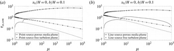
Figure 13 shows the time,
 $\unicode[STIX]{x1D70F}_{ss,wm}$
, taken to reach 99.9 % of the steady-state depth for the well-mixed model. (Results corresponding to the approximate stratified model are, except for a justifiable time offset, similar and are therefore not presented here.) Initially
 $\unicode[STIX]{x1D70F}_{ss,wm}$
increases with
 $\unicode[STIX]{x1D707}$
. However, for large
 $\unicode[STIX]{x1D707}$
, the time rate of increase of the contaminated layer depth substantially increases and the lower layer spans almost the entire box. The filling of this deep contaminated layer occurs so quickly that
 $\unicode[STIX]{x1D70F}_{ss,wm}$
later decreases with
 $\unicode[STIX]{x1D707}$
. The dashed lines of figure 13 indicate, for those cases characterized by an overshoot, the time to reach
 $\unicode[STIX]{x1D709}_{ss}$
for the first time. As noted above, the time rate of increase of
 $\unicode[STIX]{x1D709}$
is larger for larger
 $\unicode[STIX]{x1D707}$
. The time taken to first reach 99.9 % of the steady-state depth therefore monotonically decreases. Kaye & Hunt (Reference Kaye and Hunt2004) considered turbulent plume flow in emptying filling boxes devoid of porous media and observed, for intermediate
 $\unicode[STIX]{x1D707}$
, a ‘bulge’ in their predicted values for
 $\unicode[STIX]{x1D70F}_{ss,wm}$
(see their figure 8). This bulge was due to their definition of
 $\unicode[STIX]{x1D70F}_{ss,wm}$
in the context of overshoot. More specifically, they identified an overshoot as occurring if
 $\unicode[STIX]{x1D709}_{over}-\unicode[STIX]{x1D709}_{ss}>10^{-2}$
. Our threshold value is, as noted previously, smaller and we do not therefore observe a comparable bulge in figure 13. If, in this figure, we had considered either a less stringent threshold value or if we had considered still larger values for
 $\unicode[STIX]{x1D707}$
, we would observe that the overshoot eventually becomes imperceptible. At this point,
 $\unicode[STIX]{x1D70F}_{ss,wm}$
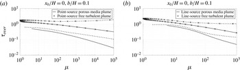
would decrease significantly, and the solid and dashed curves of figure 13 would converge. Figure 14 illustrates the time,
 $\unicode[STIX]{x1D70F}_{over}$
, taken to reach the maximum overshoot depth for both the well-mixed and approximate stratified models. Similar to
 $\unicode[STIX]{x1D70F}_{ss}$
,
 $\unicode[STIX]{x1D70F}_{over}$
is greater in case of free turbulent plumes compared to porous media plumes.
 $\unicode[STIX]{x1D70F}_{ss,wm}$
as a function of
 $\unicode[STIX]{x1D707}$
for ideal plumes with
 $b/H=0.1$
. (a) Point-source plumes and (b) line-source plumes. The solid and dashed curves correspond, respectively, to the time needed to reach 99.9 % of the steady-state depth and, for those cases having an identifiable overshoot, the initial time to reach this same elevation.

Time taken to reach the maximum overshoot depth as a function of
 $\unicode[STIX]{x1D707}$
for ideal plumes with
 $b/H=0.1$
. (a) Point-source plumes and (b) line-source plumes. The solid and dashed curves correspond to the well-mixed and approximate stratified models, respectively.

For the case of an ideal source that is turned on and off with half-period
 $\unicode[STIX]{x0394}\unicode[STIX]{x1D70F}$
, figure 15 compares the aforementioned extrema of
 $\unicode[STIX]{x1D709}$
and
 $\unicode[STIX]{x1D6FF}$
for the two plume configurations. If
 $\unicode[STIX]{x0394}\unicode[STIX]{x1D70F}$
is large enough, all of the contaminated fluid drains from the bottom of the box, which is then comprised of uniform ambient fluid, represented in figure 15(b,d) by
 $\unicode[STIX]{x1D6FF}=1$
. Similar to the previous results and for prescribed
 $\unicode[STIX]{x1D707}$
,
 $x_{0}/H$
and
 $b/H$
, the extrema of both
 $\unicode[STIX]{x1D709}$
and
 $\unicode[STIX]{x1D6FF}$
are greater for free turbulent plumes than for porous media plumes, often significantly so.
Extrema of
 $\unicode[STIX]{x1D709}$
and
 $\unicode[STIX]{x1D6FF}$
after a number of cycles for ideal free turbulent and porous media plumes. (a,b) Point-source plumes and (c,d) line-source plumes. The solid and dashed curves correspond to the well-mixed and approximate stratified models, respectively.

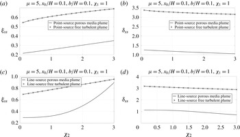
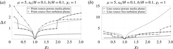
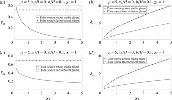
Figure 16 shows the steady-state depth and reduced gravity of the contaminated layer after changing the source volume flux while keeping the source buoyancy flux constant. From § 6, we know that increasing (decreasing) the source volume flux results in an increase (a decrease) in the steady-state depth of the contaminated layer. Figure 17 illustrates the time taken to reach 99.9 % of the steady-state depth after changing the source volume flux for both the well-mixed and approximate stratified models. Depending on the magnitude of
 $\unicode[STIX]{x1D712}_{2}$
, the contaminated layer depth may undershoot or overshoot its steady-state value. Again we apply a criterion where the difference between the magnitude of the maximum overshoot/undershoot and the steady-state depth after changing
 $Q_{0}$
must be greater than
 $10^{-3}$
. Otherwise, we do not consider an overshoot/undershoot to have occurred. There is in figure 17 therefore a pair of sudden jumps in
 $\unicode[STIX]{x0394}\unicode[STIX]{x1D70F}$
that are observed for the free turbulent plume case. For instance, in figure 17(a), such sudden jumps are observed when
 $\unicode[STIX]{x1D712}_{2}\simeq 0.25$
and
 $\unicode[STIX]{x1D712}_{2}\simeq 1.95$
for a point-source free turbulent plume with the well-mixed model. No such sudden jumps are noted in the analogue porous media case because, within the accuracy imposed by our threshold, no overshoot/undershoot occurs. It should be noted that in figure 17, the gap near
 $\unicode[STIX]{x1D712}_{2}=1$
is due to the fact that in order to accurately measure a departure from the original steady state, we used the criterion that the difference between the new and old values for
 $\unicode[STIX]{x1D709}_{ss}$
had to exceed
 $10^{-3}$
.
Steady-state depth and reduced gravity of the contaminated layer after changing the source volume flux of free turbulent and porous media plumes. (a,b) Point-source plumes and (c,d) line-source plumes.

Time taken to reach 99.9 % of the steady-state depth after changing the source volume flux of free turbulent and porous media plumes. (a) Point-source plumes and (b) line-source plumes. The solid and dashed curves correspond to the well-mixed and approximate stratified models, respectively.

Figure 18 shows the steady-state depth and reduced gravity of the contaminated layer after changing the source buoyancy flux while keeping the source volume flux constant. In the case of free turbulent plumes,
 $\unicode[STIX]{x1D707}$
is independent of the source buoyancy flux (see (2.25)). Hence, changing
 $F_{0}$
does not alter the contaminated layer steady-state depth for either source geometry. However,
 $\unicode[STIX]{x1D707}$
is a function
 $F_{0}$
in the case of porous media plumes and a change in
 $F_{0}$
therefore results in a corresponding increase or decrease in
 $\unicode[STIX]{x1D709}_{ss}$
. Because we imagine a fixed source volume flux, changes to the source buoyancy flux are synonymous with changes to the source reduced gravity. Hence, as
 $\unicode[STIX]{x1D712}_{1}$
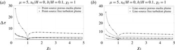
increases or decreases, so too does the contaminated layer reduced gravity. Figure 19 depicts the time taken to reach 99.9 % of the steady-state depth after changing the source buoyancy flux for both the well-mixed and approximate stratified models. As expected, it takes longer to approach steady state according to the approximate stratified model for both free turbulent and porous media plumes. Also, the porous media plumes reach steady conditions faster than the free turbulent plumes.
Contaminated layer steady-state depth and reduced gravity after changing the source buoyancy flux of free turbulent and porous media plumes. (a,b) Point-source plumes and (c,d) line-source plumes.

Time taken to reach 99.9 % of the steady-state depth after changing the source buoyancy flux of free turbulent and porous media plumes. (a) Point-source plumes and (b) line-source plumes. The solid and dashed curves correspond to the well-mixed and approximate stratified models, respectively.

8 Conclusions
The principal contribution of this study is to outline a mathematical methodology by which the emptying filling box behaviour of a control volume filled with a porous medium may be approximated. Specific reference is made to two end member cases, namely one where the contaminated layer is assumed to be uniform and another where the density of the discharged fluid is supposed to equal the plume density at the level of the interface. The predictions associated with these models typically represent upper and lower bounds; the bounds become increasingly sharp in the limit of large
 $\unicode[STIX]{x1D707}$
where
 $\unicode[STIX]{x1D707}$
is defined by the ratio of the draining time scale to the filling time scale. This ratio plays an equally critical role in the analogue and well-studied problem of an emptying filling box devoid of porous media. Indeed, the governing equations (2.21)–(2.22) appropriate to this free turbulent plume case closely resemble those germane to a laminar porous media plume (2.23)–(2.24). Our solution of these judiciously non-dimensionalized equations confirms that comparable dynamical behaviour is often observed, notwithstanding the important physical differences between laminar and turbulent plumes. For instance, we have demonstrated that for a box filled initially with ambient fluid, the contaminated layer depth may overshoot its steady-state value. Furthermore, while the well-mixed model will only predict an overshoot if
 $\unicode[STIX]{x1D707}$
exceeds a threshold value,
 $\unicode[STIX]{x1D707}_{c}$
, no such limitation applies to the approximate stratified model, which admits overshoot for small and large
 $\unicode[STIX]{x1D707}$
alike.
Results from the above research can be applied to numerous practicable situations. Consider, for instance, a short waste pile of length 200 m and width 2 m that is situated on top of saturated soil with a permeability of
 $k=10^{-11}~\text{m}^{2}$
and a porosity of
 $\unicode[STIX]{x1D719}=0.10$
. This unconfined aquifer is 100 m thick with a cross-sectional area of
 $10^{5}~\text{m}^{2}$
, and has along its base a 1 m thick confining stratum (e.g. a layer of clay) below which there exists a confined aquifer that supplies water for crop irrigation – see e.g. figure 2.11 of Todd (Reference Todd1980). We suppose that the layer of clay contains one or more fissures so that some limited communication exists between the confined and unconfined aquifers. In the presence of rainfall, we suppose that the waste pile produces a two-dimensional leachate plume having average source volume and buoyancy fluxes of
 $4.6\times 10^{-5}~\text{m}^{3}~\text{s}^{-1}$
and
 $5.3\times 10^{-10}~\text{m}^{4}~\text{s}^{-3}$
, respectively. Given these parameters, and assuming a solute molecular diffusion coefficient comparable to sodium chloride (i.e.
 $D_{m}=2.5\times 10^{-9}~\text{m}^{2}~\text{s}^{-1}$
), we estimate from figure 1(a) of Delgado (Reference Delgado2007) a dispersion coefficient of approximately
 $10^{-8}~\text{m}^{2}~\text{s}^{-1}$
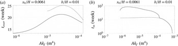
. On this basis, (a) and (b) of figure 20 respectively show the time required to reach the maximum overshoot and steady-state depths. Over a broad range of
 $Ak_{f}$
, we anticipate that
 $t_{over}\simeq 20$
weeks and
 $t_{ss}<100$
weeks, both of which seem to be quite sensible predictions in view of the spatial scales of interest here.
Time taken to reach (a) the maximum overshoot depth and (b) 99.9 % of the steady-state depth. The solid and dashed curves in (a) correspond to the well-mixed and approximate stratified models, respectively. The solid and dashed curves in (b) were both drawn assuming a well-mixed model. They correspond, respectively, to the time needed to reach 99.9 % of the steady-state depth and, for those cases having an identifiable overshoot, the time to reach this same elevation for the first time.

Our study has also considered time-varying conditions where the buoyancy source is either turned on and off with a half-period of
 $\unicode[STIX]{x0394}\unicode[STIX]{x1D70F}$
or subjected to a limited increase or decrease in the source buoyancy flux or volume flux. We showed that when the source is turned on and off periodically, the depth and reduced gravity of the contaminated layer oscillates between two extrema after a handful of cycles. In the case of an increase (decrease) in the source volume flux,
 $Q_{0}$
, the reduced gravity of the contaminated layer decreases (increases) which results in a permanent increase (decrease) in the contaminated layer depth. Different behaviour is noted when adjusting the source buoyancy flux,
 $F_{0}$
, at least when considering boxes devoid of porous media. The contaminated layer depth is then independent of
 $F_{0}$
and so the original depth is recovered after some transient adjustment phase. On the other hand, the steady-state depth of the contaminated layer is a function of
 $F_{0}$
for porous media plumes; thus, a change in the source buoyancy flux leads to a permanent change of interface depth, analogous to the case where
 $Q_{0}$
is altered.
Acknowledgement
Funding for this study was generously provided by the Natural Science and Engineering Research Council (NSERC). This paper is dedicated to Professor Paul F. Linden on the occasion of his 70th birthday.