1 Introduction
Rotation plays an important role in engineering, geophysical and astrophysical fluid motions. It induces inertial waves of which the Coriolis force acts as the restoring force (Greenspan Reference Greenspan1968). The dispersion relationship for an inertial wave is
 $$\begin{eqnarray}{\it\sigma}=\pm \frac{2{\it\bf\Omega}\boldsymbol{\cdot }\boldsymbol{k}}{k},\end{eqnarray}$$
where
 ${\it\sigma}$
is the wave frequency,
 $\boldsymbol{k}$
the wavevector and
 ${\it\bf\Omega}$
the angular velocity of rotation. This expression shows that the frequency of the inertial wave is in the range
 $|{\it\sigma}|\leqslant 2{\it\Omega}$
. An inertial wave is dispersive and its group velocity is perpendicular to its phase velocity. An inertial wave carries energy and angular momentum in the interior of fluid and then dissipates through viscosity. Moreover, it has helical structure, which favours the dynamo action for generating magnetic field (e.g. Moffatt Reference Moffatt1970a
,Reference Moffatt
b
; Davidson Reference Davidson2014; Wei Reference Wei2014, etc.).
In the geometry of an annular channel, the problem of inertial waves was studied by Cui, Zhang & Liao (Reference Cui, Zhang and Liao2014), and in the spherical geometry it has been extensively studied by, among others, Hollerbach & Kerswell (Reference Hollerbach and Kerswell1995), Rieutord & Valdettaro (Reference Rieutord and Valdettaro1997), Ogilvie (Reference Ogilvie2005) and Tilgner (Reference Tilgner2007a ). Because of the singularity of the Poincaré equation, i.e. the governing equation of inertial waves, the inertial waves in spherical geometry are spawned from the critical latitude and then propagate and reflect in the thin shear layers, i.e. the wave attractors (Ogilvie Reference Ogilvie2005). In the Earth’s fluid core, the inertial waves driven by precession are discussed by Busse (Reference Busse1968), Kerswell (Reference Kerswell1993), Lorenzani & Tilgner (Reference Lorenzani and Tilgner2001, Reference Lorenzani and Tilgner2003), Tilgner (Reference Tilgner and Schubert2007b ) and Zhang, Chan & Liao (Reference Zhang, Chan and Liao2014).
Inertial waves can be excited by tidal forces in planetary and stellar interiors. Tides exist widely in astronomical binary systems, e.g. the Earth and the Moon, a giant planet and its satellite, a host star and an exoplanet, binary normal stars or white dwarfs. In the binary system, one body (primary) is gravitationally perturbed by the other (companion) such that the primary deforms and produces the tidal bulge pointing to the companion. Tidal torque transfers angular momentum between the orbital motion and the rotational motion of binaries, and dissipation in the planetary and stellar interiors plays an important role for the angular momentum transfer. Waves can be excited by the harmonic tidal force, i.e. the dynamical tide, and the dissipation of these waves is very efficient because of their small scales. Particularly, the inertial waves induced by the tidal force, i.e. the dynamical tide arising from rotation, are discussed by Kerswell (Reference Kerswell1994), Kumar & Goodman (Reference Kumar and Goodman1996) and Ogilvie (Reference Ogilvie2014). Tidally excited inertial waves dissipate through viscosity, and the tidal dissipation becomes very strong when resonance occurs, namely the tidal frequency is close to the eigenfrequency of the inertial wave in the unforced rotating flow. There are infinite inertial eigenmodes in spherical geometry and therefore the tidal resonance is prone to occur as long as the tidal frequency is less than twice the rotation frequency. In the nonlinear regime, i.e. with the presence of nonlinear inertial force, it was pointed out by Tilgner (Reference Tilgner2007a ) that the inertial waves can generate zonal flow. In addition, the nonlinear wave breaking has a significant effect on the tidal dissipation (Kumar & Goodman Reference Kumar and Goodman1996). The nonlinear tidal flow was numerically studied by Favier et al. (Reference Favier, Barker, Baruteau and Ogilvie2014) with the boundary radial flow method and by Cébron & Hollerbach (Reference Cébron and Hollerbach2014) with the body force method. Although the linear regime has been extensively studied, the nonlinear regime is not well understood, e.g. the scaling law of tidal dissipation versus Ekman number is unknown (Favier et al. (Reference Favier, Barker, Baruteau and Ogilvie2014) studied a little about the scaling laws, see their figure 4, but their study is at non-resonant frequencies and the nonlinear dissipation at the resonant frequency is still unknown). In our study we will focus on the nonlinear effect at both resonant and non-resonant frequencies.
In this short paper, we will study the rotating flow driven by the harmonic force in a periodic box, i.e. a cubic box with a periodic boundary condition, which is a toy model for a small piece of region in a container (for engineering) or a star (for astrophysics). Not as in the spherical geometry, the inertial waves in a periodic box do not reflect but propagate forwards, and hence do not focus in the thin shear layers. In § 2 the equations are given. In § 3 the linear regime is analytically studied and the dissipation at the resonant frequency is derived. In § 4 the nonlinear regime is numerically studied and compared to the linear regime. In § 5 a brief summary is given.
2 Equations
We study the rotating flow of an incompressible fluid in a periodic box with size
 $2{\rm\pi}l$
. We use the Cartesian coordinate system
 $(x,y,z)$
and the uniform rotation is imposed in the
 $z$
direction. In the frame rotating at the angular velocity
 ${\it\bf\Omega}={\it\Omega}\hat{\boldsymbol{z}}$
, the dimensionless Navier–Stokes equation of fluid motion reads
 $$\begin{eqnarray}\frac{\partial \boldsymbol{u}}{\partial t}+\boldsymbol{u}\boldsymbol{\cdot }\boldsymbol{{\rm\nabla}}\boldsymbol{u}=-\boldsymbol{{\rm\nabla}}p+E{\rm\nabla}^{2}\boldsymbol{u}+2\boldsymbol{u}\times \hat{\boldsymbol{z}}+\boldsymbol{f},\end{eqnarray}$$
where length is normalised with
 $l$
, time with the inverse of rotation frequency
 ${\it\Omega}^{-1}$
and velocity with
 ${\it\Omega}l$
. The Ekman number
 $E={\it\nu}/({\it\Omega}l^{2})$
, where
 ${\it\nu}$
is viscosity, measures the ratio of rotational time scale to viscous time scale.
The driving force is assumed to be a single travelling wave, i.e.
 $$\begin{eqnarray}\boldsymbol{f}=\text{Re}\{\hat{\boldsymbol{f}}\text{e}^{\text{i}(\boldsymbol{k}\boldsymbol{\cdot }\boldsymbol{x}-{\it\omega}t)}\},\end{eqnarray}$$
where
 $\hat{\boldsymbol{f}}$
is the complex force amplitude,
 $\boldsymbol{k}$
the force wavevector,
 ${\it\omega}$
the force frequency and
 $\text{Re}$
denotes taking the real part. The tidal force exerted by the companion on the primary is the difference between the force on any point and the force at the centre of the primary, and the tidal potential is the superposition of spherical harmonics with the time dependence on the Doppler-shifted frequency (Souchay, Mathis & Tokieda Reference Souchay, Mathis and Tokieda2013; Ogilvie Reference Ogilvie2014). Although the total tidal force is curl-free, its contribution to the dynamical tide is vortical because of the very slow equilibrium tide; see the details in appendix B of Ogilvie (Reference Ogilvie2005). Briefly speaking, the incompressible equilibrium tide varies slowly and does not satisfy the hydrostatic balance such that the residual is a vortical force that can drive the dynamical tide, e.g. the inertial waves in a rotating fluid. In our simplified model,
 $\boldsymbol{f}$
corresponds to the force responsible for the dynamical tide and it is not curl-free. On the other hand, to have the dynamical effect on flow, the driving force
 $\boldsymbol{f}$
should not be curl-free (if it is curl-free then it can be absorbed into the pressure gradient to act as an additional pressure). For the simplicity to derive the solution in the linear regime (see § 3), we assume it to be a helical force, i.e.
 $\boldsymbol{{\rm\nabla}}\times \boldsymbol{f}=k\boldsymbol{f}$
where
 $k=|\boldsymbol{k}|$
is the force wavenumber. One may argue that the helical force is too artificial. Here we give more explanation. Any vector field can be decomposed into a curl-free part and a divergence-free part, i.e. the Helmholtz decomposition. Moreover, the divergence-free part can be decomposed into helical modes (see Waleffe Reference Waleffe1992). Back to the driving force
 $\boldsymbol{f}$
, the curl-free part can be absorbed into the pressure gradient and the divergence-free part can be expressed as the superposition of helical forces. This is the reason that we use the helical force for the study of tidal waves. In the spectral space the helical force satisfies
 $$\begin{eqnarray}\text{i}\boldsymbol{k}\times \hat{\boldsymbol{f}}=k\hat{\boldsymbol{f}}.\end{eqnarray}$$
Equation (2.3) is degenerate (i.e. only two components are independent) and yields
 $$\begin{eqnarray}\frac{\hat{f}_{y}}{\hat{f}_{x}}=\frac{-k_{x}k_{y}+\text{i}kk_{z}}{k_{y}^{2}+k_{z}^{2}},\quad \frac{\hat{f}_{z}}{\hat{f}_{y}}=\frac{-k_{y}k_{z}+\text{i}kk_{x}}{k_{z}^{2}+k_{x}^{2}},\quad \frac{\hat{f}_{x}}{\hat{f}_{z}}=\frac{-k_{z}k_{x}+\text{i}kk_{y}}{k_{x}^{2}+k_{y}^{2}}.\end{eqnarray}$$
We denote the modulus of the complex force amplitude by
 $a$
, i.e.
 $$\begin{eqnarray}|\hat{\boldsymbol{f}}|=\sqrt{|\,\hat{f}_{x}|^{2}+|\,\hat{f}_{y}|^{2}+|\,\hat{f}_{z}|^{2}}=a.\end{eqnarray}$$
Equations (2.4) and (2.5) then combine to yield
 $$\begin{eqnarray}|\,\hat{f}_{x}|=\frac{\sqrt{k_{y}^{2}+k_{z}^{2}}}{\sqrt{2}k}a,\quad |\,\hat{f}_{y}|=\frac{\sqrt{k_{z}^{2}+k_{x}^{2}}}{\sqrt{2}k}a,\quad |\,\hat{f}_{z}|=\frac{\sqrt{k_{x}^{2}+k_{y}^{2}}}{\sqrt{2}k}a,\end{eqnarray}$$
and, in addition, the arguments of
 $\hat{f}_{y}/\hat{f}_{x}$
and
 $\hat{f}_{z}/\hat{f}_{x}$
are, respectively,
 $$\begin{eqnarray}{\rm\pi}-\arccos \frac{k_{x}k_{y}}{\sqrt{(k_{y}^{2}+k_{z}^{2})(k_{z}^{2}+k_{x}^{2})}},\quad {\rm\pi}+\arccos \frac{k_{z}k_{x}}{\sqrt{(k_{x}^{2}+k_{y}^{2})(k_{y}^{2}+k_{z}^{2})}}.\end{eqnarray}$$
The arguments of
 $\hat{f}_{x}$
,
 $\hat{f}_{y}$
and
 $\hat{f}_{z}$
themselves are insignificant for the volume integral of energy and dissipation, but the differences between them (i.e. phase shifts) do matter, and without loss of generality the argument of
 $\hat{f}_{x}$
is given to be
 $0$
. Thus, (2.6) and (2.7) give the three components of the complex amplitude
 $\hat{\boldsymbol{f}}$
, and (2.2) gives the driving force in physical space.
The output that we are concerned with is the volume-averaged dissipation. With the periodic boundary condition, it is proportional to enstrophy, i.e.
 $$\begin{eqnarray}D=E\frac{1}{V}\int _{V}|\boldsymbol{{\rm\nabla}}\times \boldsymbol{u}|^{2}\,\text{d}V=\frac{E}{2}|\text{i}\boldsymbol{k}\times \hat{\boldsymbol{u}}|^{2}.\end{eqnarray}$$
The numerical calculations are carried out with the pseudo-spectral code using fast Fourier transformation. The resolution is checked with two methods. One is to double the resolution until the total energy and enstrophy have no noticeable change. The other is to see whether the energy and enstrophy spectra decay by sufficient (say, more than 10) magnitudes. In our regime of moderate parameters, resolutions as high as
 $128^{3}$
are used.
3 Linear regime
In the absence of a nonlinear inertial force, we can analytically solve the linearised Navier–Stokes equation
 $$\begin{eqnarray}\frac{\partial \boldsymbol{u}}{\partial t}=-\boldsymbol{{\rm\nabla}}p+E{\rm\nabla}^{2}\boldsymbol{u}+2\boldsymbol{u}\times \hat{\boldsymbol{z}}+\boldsymbol{f}.\end{eqnarray}$$
Because the driving force is a single harmonic (equation (2.2)), the solution to the linear equation is assumed to be
 $\boldsymbol{u}=\text{Re}\{\hat{\boldsymbol{u}}\text{e}^{\text{i}(\boldsymbol{k}\boldsymbol{\cdot }\boldsymbol{x}-{\it\omega}t)}\}$
and
 $p=\text{Re}\{\hat{p}\text{e}^{\text{i}(\boldsymbol{k}\boldsymbol{\cdot }\boldsymbol{x}-{\it\omega}t)}\}$
. Substitution into (3.1) yields
 $$\begin{eqnarray}-\text{i}{\it\omega}\hat{\boldsymbol{u}}=-\text{i}\boldsymbol{k}\hat{p}-Ek^{2}\hat{\boldsymbol{u}}+2\hat{\boldsymbol{u}}\times \hat{\boldsymbol{z}}+\hat{\boldsymbol{f}}.\end{eqnarray}$$
By performing
 $\text{i}\boldsymbol{k}\times$
on the above equation to eliminate pressure and applying
 $\text{i}\boldsymbol{k}\boldsymbol{\cdot }\hat{\boldsymbol{u}}=0$
(incompressible flow) and
 $\text{i}\boldsymbol{k}\times \hat{\boldsymbol{f}}=k\hat{\boldsymbol{f}}$
(helical force), we derive
 $$\begin{eqnarray}({\it\omega}+\text{i}Ek^{2})\boldsymbol{k}\times \hat{\boldsymbol{u}}=2\text{i}k_{z}\hat{\boldsymbol{u}}+k\hat{\boldsymbol{f}}.\end{eqnarray}$$
Performing again
 $\text{i}\boldsymbol{k}\times$
on the above equation yields
 $$\begin{eqnarray}k^{2}({\it\omega}+\text{i}Ek^{2})\hat{\boldsymbol{u}}=-2\text{i}k_{z}\boldsymbol{k}\times \hat{\boldsymbol{u}}+\text{i}k^{2}\hat{\boldsymbol{f}}.\end{eqnarray}$$
Combining the above two equations to eliminate
 $\text{i}\boldsymbol{k}\times \hat{\boldsymbol{u}}$
, we are led to
 $$\begin{eqnarray}[(2k_{z})^{2}-k^{2}({\it\omega}+\text{i}Ek^{2})^{2}]\hat{\boldsymbol{u}}=\text{i}k[2k_{z}-k({\it\omega}+\text{i}Ek^{2})]\hat{\boldsymbol{f}}.\end{eqnarray}$$
When the driving force is absent (
 $\hat{\boldsymbol{f}}=\mathbf{0}$
) and viscosity vanishes (
 $E=0$
), (3.5) reduces to the dispersion relationship for an inertial wave, i.e.
 ${\it\sigma}=\pm 2k_{z}/k$
(where the eigenfrequency is denoted by
 ${\it\sigma}$
). Because the factor
 $[2k_{z}-k({\it\omega}+\text{i}Ek^{2})]$
can never be zero due to the phase shift caused by viscosity, it is cancelled and we derive
 $$\begin{eqnarray}\hat{\boldsymbol{u}}=\frac{\text{i}k\hat{\boldsymbol{f}}}{2k_{z}+k({\it\omega}+\text{i}Ek^{2})}.\end{eqnarray}$$
Equation (3.6) is the solution to the linearised Navier–Stokes equation (3.1). By virtue of (2.8), dissipation can be calculated as
 $$\begin{eqnarray}D=\frac{E}{2}|\text{i}\boldsymbol{k}\times \hat{\boldsymbol{u}}|^{2}=\frac{E}{2}\frac{a^{2}k^{4}}{|2k_{z}+k({\it\omega}+\text{i}Ek^{2})|^{2}}.\end{eqnarray}$$
Resonance occurs when the linear response (3.6) is singular with the neglect of viscosity. In the presence of viscosity, the linear response (3.6) becomes very strong at the frequency
 $$\begin{eqnarray}{\it\omega}=-\frac{2k_{z}}{k},\end{eqnarray}$$
which is called the resonant frequency. Substitution of (3.8) into (3.6) leads to the response at the resonant frequency
 $$\begin{eqnarray}\hat{\boldsymbol{u}}=\frac{1}{Ek^{2}}\hat{\boldsymbol{f}}.\end{eqnarray}$$
Substitution of (3.8) into (3.7) leads to the dissipation at the resonance frequency
 $$\begin{eqnarray}D=\frac{a^{2}}{2Ek^{2}}.\end{eqnarray}$$
Therefore, the dissipation at the resonant frequency scales as
 $$\begin{eqnarray}D\propto E^{-1}k^{-2}.\end{eqnarray}$$
According to (3.7), we can calculate the dissipation of the linear response. For the linear response we fix
 $a=1$
. Firstly we study the effect of the force frequency on the linear response. We calculate at the four Ekman numbers
 $10^{-3}$
,
 $10^{-4}$
,
 $10^{-5}$
and
 $10^{-6}$
, and at the fixed wavenumbers
 $k_{x}=k_{y}=k_{z}=1$
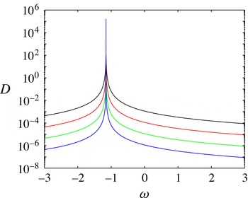
. Figure 1 shows the dissipation versus the force frequency. It is verified that the dissipation has a sharp peak at the resonant frequency
 ${\it\omega}=-2k_{z}/k=-2/\sqrt{3}\approx -1.1547$
. It also indicates that a lower Ekman number corresponds to a higher peak, which is consistent with (3.11). We pick out two representative frequencies. One frequency is
 ${\it\omega}=-1.16$
, which is considered to be near the resonant frequency (e.g. at
 $E=10^{-3}$
the dissipation at
 ${\it\omega}=-1.16$
is 24 % of the dissipation at the resonant frequency). The other is
 ${\it\omega}=-1.2$
, which is considered to be far away from the resonant frequency (e.g. at
 $E=10^{-3}$
the dissipation at
 ${\it\omega}=-1.2$
is 0.44 % of the dissipation at the resonant frequency). In the following calculations throughout this paper, we will often use these two representative frequencies.
The investigation of the force frequency in the linear regime. The dissipation
 $D$
versus the force frequency
 ${\it\omega}$
, for
 $a=1$
and
 $k_{x}=k_{y}=k_{z}=1$
. Black, red, green and blue lines (from top downwards) denote, respectively,
 $E=10^{-3}$
,
 $10^{-4}$
,
 $10^{-5}$
and
 $10^{-6}$
.

Next we study the effect of the force wavenumber on the linear response. We calculate at the four Ekman numbers as in the last paragraph and at three frequencies, namely the resonant frequency
 ${\it\omega}=-2/\sqrt{3}$
,
 ${\it\omega}=-1.16$
near the resonant frequency, and
 ${\it\omega}=-1.2$
far away from the resonant frequency. The resonant frequency depends on the orientation of the wavevector. To keep the resonant frequency fixed, we keep
 $k_{x}=k_{y}=k_{z}$
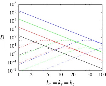
. Figure 2 shows the dissipation versus the force wavenumber. It is verified that the dissipation scales as
 $D\propto k^{-2}$
at the resonant frequency, as predicted by (3.11). When the force wavenumber is sufficiently large, the dissipation at the other frequencies converges to the dissipation at the resonant frequency. This suggests that the dissipation at the resonant frequency is much stronger than the dissipation at the non-resonant frequency on the large scales.
The investigation of the force wavenumber in the linear regime. The dissipation
 $D$
versus the force wavenumber
 $k_{x}=k_{y}=k_{z}$
, for
 $a=1$
. Black, red, green and blue lines (from bottom upwards for the straight lines) denote, respectively,
 $E=10^{-3}$
,
 $10^{-4}$
,
 $10^{-5}$
and
 $10^{-6}$
. Solid lines denote the resonant frequency
 ${\it\omega}=-2/\sqrt{3}$
, dashed lines
 ${\it\omega}=-1.16$
near the resonant frequency, and dash-dotted lines
 ${\it\omega}=-1.2$
far away from the resonant frequency.

We then study the effect of the Ekman number on the linear response. Since we know that the resonance has a striking effect on the large scales, we fix
 $k_{x}=k_{y}=k_{z}=1$
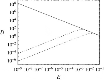
. Figure 3 shows the dissipation versus
 $E$
at the three frequencies. It indicates that the dissipation at the resonant frequency scales as
 $D\propto E^{-1}$
, as predicted by (3.11). The dissipation at the other frequencies scales as
 $D\propto E$
in the regime of low Ekman number and converges to the dissipation at the resonant frequency in the regime of high Ekman number. This suggests that the dissipation at the resonant frequency is much stronger than the dissipation at the non-resonant frequencies at the low Ekman numbers.
In addition, we also carried out the direct numerical calculations of (3.1) and the relative error of the numerical calculations compared to the analytical results is within 0.01 %.
The investigation of the Ekman number in the linear regime. The dissipation
 $D$
versus the Ekman number
 $E$
, for
 $a=1$
and
 $k_{x}=k_{y}=k_{z}=1$
. Solid line denotes
 ${\it\omega}=-2/\sqrt{3}$
, dashed line
 ${\it\omega}=-1.16$
near the resonant frequency, and dash-dotted line
 ${\it\omega}=-1.2$
far away from the resonant frequency.

4 Nonlinear regime
We now numerically study the nonlinear regime, i.e. solving (2.1). Firstly we study the nonlinear effect due to the force amplitude. We gradually increase the force amplitude
 $a$
from
 $1\times 10^{-3}$
to
 $2\times 10^{-3}$
and then to
 $3\times 10^{-3}$
. The stronger force drives a stronger flow and hence higher dissipation, and so we normalise the dissipation with
 $a^{2}$
, which reflects the nonlinear effect on the dissipation and we call
 $D/a^{2}$
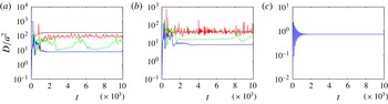
the effective dissipation. Figure 4 shows the effective dissipation
 $D/a^{2}$
versus time for the three amplitudes,
 $1\times 10^{-3}$
,
 $2\times 10^{-3}$
and
 $3\times 10^{-3}$
, at
 $E=1\times 10^{-3}$
. Three different frequencies are studied, i.e. the resonant frequency
 ${\it\omega}=-2/\sqrt{3}\approx -1.1547$
,
 ${\it\omega}=-1.16$
near the resonant frequency, and
 ${\it\omega}=-1.2$
far away from the resonant frequency. The linear results are also shown in the figure for comparison with the nonlinear results. Figure 4(a) shows that at the resonant frequency the effective dissipation is lower than in the linear regime and it decreases with increasing force amplitude, namely the stronger nonlinearity has a greater suppression effect on the effective dissipation. It is interesting that rapid fluctuations occur with
 $a=1\times 10^{-3}$
while the linear result has no such fluctuations. Evidently these fluctuations arise from some instabilities caused by the nonlinearity. They become less frequent with
 $a=2\times 10^{-3}$
and vanish with
 $a=3\times 10^{-3}$
. Figure 4(b) shows that near the resonant frequency this nonlinear suppression for dissipation still exists but becomes weaker, e.g. the black line (the linear regime) and the time average of the unsteady red line (the weakest nonlinear regime) almost overlap. Figure 4(c) shows that far away from the resonant frequency the nonlinear suppression is absent, namely the black, red, green and blue lines completely overlap. This is because the flow amplitude at a frequency far away from the resonant frequency is too small to have a strong nonlinear effect. In summary, the nonlinear effect suppresses the effective dissipation at the resonant frequency and this suppression effect is still significant near the resonant frequency but negligible far away from the resonant frequency.
The investigation of the force amplitude in the nonlinear regime. The normalised dissipation
 $D/a^{2}$
versus time at
 $E=1\times 10^{-3}$
with
 $k_{x}=k_{y}=k_{z}=1$
. (a) The resonant frequency
 ${\it\omega}=-2/\sqrt{3}$
. (b) Frequency
 ${\it\omega}=-1.16$
near the resonant frequency. (c) Frequency
 ${\it\omega}=-1.2$
far away from the resonant frequency. Black lines (uppermost in (a)) denote the results in the linear regime. Red, green and blue lines (from top downwards) denote the nonlinear regime with, respectively,
 $a=1\times 10^{-3}$
,
 $2\times 10^{-3}$
and
 $3\times 10^{-3}$
.

To better understand the nonlinear effect on the dissipation, we investigate the dependence of the dissipation on the Rossby number, which measures the relative strength of the inertial force and the Coriolis force. The Rossby number is defined as
 $Ro=U/(l{\it\Omega})$
where
 $U$
is the characteristic velocity. We take
 $U$
to be the square root of the volume-averaged kinetic energy, and under our normalisation the Rossby number is exactly the dimensionless
 $U$
, i.e.
 $$\begin{eqnarray}Ro=\sqrt{\frac{1}{V}\int u^{2}\,\text{d}V}.\end{eqnarray}$$
For the fluctuating flows, we take the time average in the statistically steady state (after the initial transient growth stage) to calculate
 $Ro$
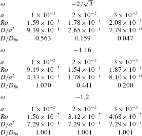
. Table 1 shows
 $Ro$
and
 $D/a^{2}$
versus
 $a$
at the three frequencies. It indicates that at the fixed frequency the larger force amplitude leads to a stronger nonlinearity (
 $Ro$
) and hence weaker
 $D/a^{2}$
. The last row in each block shows the ratio of the nonlinear dissipation to the corresponding linear dissipation, which clearly reveals that the nonlinear suppression is very strong at the resonant frequency for the large force amplitude. At the resonant frequency, the stronger force amplitude leads to the lower ratio. When the force frequency departs farther away from the resonant frequency, the nonlinearity becomes weaker.
The nonlinear regime. The time-averaged
 $Ro$
,
 $D/a^{2}$
and
 $D/D_{lin}$
versus
 ${\it\omega}$
and
 $a$
in figure 4.

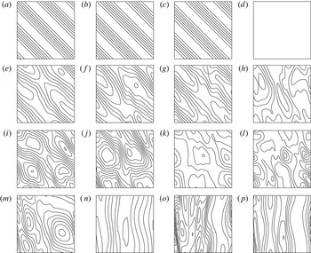
Figure 5 shows the velocity structure at the resonant frequency
 ${\it\omega}=-2/\sqrt{3}$
. With
 $a=1\times 10^{-3}$
the main flow structure has the basic flow of
 $k_{x}=k_{y}=k_{z}=1$
(figure 5
a–d) and the instabilities on top of the basic flow (figure 5
e–h); with
 $a=2\times 10^{-3}$
the structure of the basic flow alters due to the strong nonlinearity (figure 5
i–l); and at
 $a=3\times 10^{-3}$
the structure of the basic flow completely disappears and the
 $z$
-independent structure emerges (figure 5
m–p).
The contours of velocity in the
 $x{-}z$
plane at
 $y=0$
for the snapshot at time
 $=$
10 000. In each row the panels from left to right are contours of respectively
 $u_{1}$
(a,e,i,m),
 $u_{2}$
(b,f,j,n),
 $u_{3}$
(c,g,k,o) and kinetic energy (d,h,l,p). At the resonant frequency,
 ${\it\omega}=-2/\sqrt{3}$
corresponding to figure 4(a). (a–d) Linear response with
 $a=1\times 10^{-3}$
(kinetic energy is constant). (e–h) Nonlinear response with
 $a=1\times 10^{-3}$
. (i–l) Nonlinear response with
 $a=2\times 10^{-3}$
. (m–p) Nonlinear response with
 $a=3\times 10^{-3}$
.

Next we investigate the force wavenumber. In the linear regime, the dissipation scales as
 $k^{-2}$
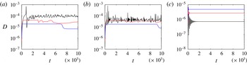
at the resonant frequency and it is much stronger than the dissipation at the non-resonant frequencies on the large scales (see figure 2). In the nonlinear regime, figure 6 shows the dissipation versus time for the three wavenumbers,
 $k_{x}=k_{y}=k_{z}=1$
,
 $2$
and
 $3$
, with the three frequencies as in figure 4. At the resonant frequency (figure 6
a), the higher wavenumber leads to lower dissipation, which is consistent with the prediction in the linear regime (the solid black line in figure 2). At the frequency near the resonant frequency (figure 6
b), the higher wavenumber leads to lower dissipation, which is also consistent with the prediction in the linear regime (the dashed black line in figure 2). At the frequency far away from the resonant frequency (figure 6
c), the higher wavenumber leads to higher dissipation, which is again consistent with the prediction in the linear regime (the dash-dotted black line in figure 2).
The investigation of the force wavenumber in the nonlinear regime. The dissipation
 $D$
versus time at
 $E=1\times 10^{-3}$
with
 $a=1\times 10^{-3}$
. (a) The resonant frequency
 ${\it\omega}=-2/\sqrt{3}$
. (b) Frequency
 ${\it\omega}=-1.16$
near the resonant frequency. (c) Frequency
 ${\it\omega}=-1.2$
far away from the resonant frequency. Black (uppermost in (a)), red (middle) and blue lines (lowermost in (a)) denote the nonlinear regime with respectively
 $k_{x}=k_{y}=k_{z}=1$
,
 $2$
and
 $3$
. (Lines are in opposite order in (c)).

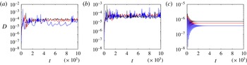
We then investigate the Ekman number. Usually viscosity has a stabilising effect (rigorously speaking, viscosity can be both stabilising and destabilising, e.g. in a parallel shear flow it can destabilise the inviscid flow with parabolic profile), and therefore, when the Ekman number decreases, the nonlinear effect becomes significant. Figure 7 shows the dissipation versus time for the three different Ekman numbers, i.e.
 $1\times 10^{-3}$
,
 $7.5\times 10^{-4}$
and
 $5\times 10^{-4}$
, with the three frequencies as in figure 4. Figure 7(a) shows that at the resonant frequency the lower Ekman number leads to lower dissipation. This is opposite to the prediction in the linear regime, namely the lower Ekman number leads to higher dissipation at the resonant frequency, as shown by the solid line in figure 3. A tentative interpretation is that at the resonant frequency the lower Ekman number gives rise to stronger nonlinear suppression for dissipation, which wins out over the linear enhancement for dissipation. Figure 7(b) shows that near the resonant frequency the high and low Ekman numbers do not seem to have a significant difference in respect of the time-averaged dissipation but the lower Ekman number leads to a stronger amplitude of oscillations of dissipation, which is presumably the instabilities caused by the stronger nonlinearity. Figure 7(c) shows that far away from the resonant frequency the lower Ekman number leads to lower dissipation. Moreover, the ratio of the three dissipations at
 $E=1\times 10^{-3}$
,
 $7.5\times 10^{-4}$
and
 $5\times 10^{-4}$
is
 $1:0.75:0.5$
, which is consistent with the prediction of
 $D\propto E$
in the linear regime as shown by the dash-dotted line in figure 3. This again indicates that the nonlinear effect is negligible far away from the resonant frequency.
The investigation of the Ekman number in the nonlinear regime. The dissipation
 $D$
versus time with
 $a=1\times 10^{-3}$
and
 $k_{x}=k_{y}=k_{z}=1$
. (a) The resonant frequency
 ${\it\omega}=-2/\sqrt{3}$
. (b) Frequency
 ${\it\omega}=-1.16$
near the resonant frequency. (c) Frequency
 ${\it\omega}=-1.2$
far away from the resonant frequency. Black, red and blue lines (from top downwards in (c)) denote the nonlinear regime at respectively
 $E=1\times 10^{-3}$
,
 $7.5\times 10^{-4}$
and
 $5\times 10^{-4}$
.

5 Conclusion
In this work, we study analytically and numerically the rotating flow driven by a harmonic force. In the linear regime we analytically derive the response to the harmonic force and the dissipation. The dissipation scales as
 $D\propto E^{-1}k^{-2}$
at the resonant frequency and
 $D\propto E$
at other non-resonant frequencies. In the nonlinear regime we do the numerical calculations and compare with the linear regime. It is found that the effective dissipation (
 $D/a^{2}$
) at the resonant frequency in the nonlinear regime is lower than in the linear regime and decreases with increasing force amplitude; however, this nonlinear suppression is negligible far away from the resonant frequency. Opposite to the linear regime, the lower Ekman number leads to lower dissipation at the resonant frequency because of the stronger nonlinear effect. This nonlinear effect can be interpreted. At the resonant frequency, if the tidal force amplitude is large enough or the Ekman number is small enough, the nonlinear inertial force (
 $\boldsymbol{u}\boldsymbol{\cdot }\boldsymbol{{\rm\nabla}}\boldsymbol{u}$
) takes effect, such that the flow is suppressed, namely the flow intensity is weaker than without the nonlinear inertial force. Hence, the dissipation, which is equal to the enstrophy multiplied by viscosity, is also suppressed. Far away from the resonant frequency, the tidal response is weak and therefore the nonlinear effect is not striking.
In summary, when the frequency of the external harmonic force is close to the negative frequency of the inertial wave in the unforced rotating flow, the dissipation can be greatly enhanced but the stronger nonlinear effect due to the stronger force amplitude or the lower Ekman number can suppress this enhancement; however, the dissipation at a frequency far away from the resonant frequency is small and the nonlinear effect is insignificant. Our numerical calculations about the nonlinear effect on the dynamical tide imply that the previous linear calculations have overestimated the tidal dissipation at the resonant frequency.
Acknowledgement
This work was initiated in Princeton and completed in Shanghai. I am financially supported by the National Science Foundations Center for Magnetic Self-Organization under grant PHY-0821899 and the startup grant of Shanghai Jiaotong University.