2 XGCa model with impurities

Even though most of the description given in this section is common to the total-f XGC family of codes, we will use the name XGCa in this paper since XGCa is what is used in this study. XGCa is a total-f (Ku et al. Reference Ku, Chang, Hager, Churchill, Tynan, Cziegler, Greenwald, Hughes, Parker and Adams2018) gyrokinetic particle-in-cell (PIC) code that is able to simulate large and small scale physics together. XGCa uses a hybrid-Lagrangian scheme in which the slow space–time varying component of the distribution function is gradually taken out from the particles and moved to a five-dimensional phase-space grid, see Ku et al. (Reference Ku, Hager, Chang, Kwon and Parker2016, Reference Ku, Chang, Hager, Churchill, Tynan, Cziegler, Greenwald, Hughes, Parker and Adams2018). This technique permits us to control the particle noise by mitigating the weight growth in the particle part of the distribution function, $f_{p}$ . The distribution function $f$ is composed of an analytic input part $f_{a}$ , a grid part $f_{g}$ , and a particle part $f_{p}$ , such that $f=f^{a}+f^{g}+f^{p}$ : see the detailed discussion in Ku et al. (Reference Ku, Hager, Chang, Kwon and Parker2016, Reference Ku, Chang, Hager, Churchill, Tynan, Cziegler, Greenwald, Hughes, Parker and Adams2018).

The XGC family of codes, including XGCa, uses the same new multi-species full-f Fokker–Plank operator in Landau form evaluated on a five-dimensional (5-D) phase-space grid (Hager & Chang Reference Hager and Chang2016)

(2.1) $$\begin{eqnarray}\displaystyle {\mathcal{C}}_{s}=\mathop{\sum }_{s^{\prime }}{\mathcal{C}}[f_{s},f_{s^{\prime }}], & & \displaystyle\end{eqnarray}$$

where the subscripts denote particle species. Collisions are computed between all pairs of species $(s,s^{\prime })$ and evaluated with the total-f distribution function $f_{s}$ . The complexity of the collision operator is quadratic with the number of species. This significantly increases the cost of simulations when many ion species are simulated.

In XGCa, the main and impurity ions are treated gyrokinetically. The only restriction in XGCa (‘a’ stands for axisymmetric) compared to the main version XGC (often called XGC1) is that only the axisymmetric (toroidal Fourier mode number $n=0$ ) component of the electrostatic field is kept in XGCa (Hager et al. Reference Hager, Yoon, Ku, D’Azevedo, Worley and Chang2016). Therefore, the grid is simplified and XGCa simulations are computationally less expensive than XGC1 simulations.

The gyrokinetic Poisson equation, ${\mathcal{L}}\unicode[STIX]{x1D719}=\bar{n}$ , is solved when accounting for all ion-species contributions

(2.2) $$\begin{eqnarray}\displaystyle & \displaystyle \left(\mathop{\sum }_{s\in \{\text{ions}\}}{\mathcal{L}}_{s}\right)\unicode[STIX]{x1D719}=\mathop{\sum }_{s\in \{\text{ions},\text{e}-\}}\bar{n}_{s}, & \displaystyle\end{eqnarray}$$

with ${\mathcal{L}}_{s}$ the gyrokinetic polarization operator describing the polarization part of the ion-species density. All ions, i.e. main and impurity, and electron contributions are accounted for. Electrons are drift kinetic. See Ku et al. (Reference Ku, Chang, Hager, Churchill, Tynan, Cziegler, Greenwald, Hughes, Parker and Adams2018) for details about the original pure plasma Poisson solver which is implemented in XGC.

The same grid of gyroaveraging matrices is used for every ion species. Indeed, to compute the ion density, we first sum the gyrocentre charge density of all ion species on the same 4-D grid by computing

(2.3) $$\begin{eqnarray}\displaystyle & \displaystyle n(\boldsymbol{X},\unicode[STIX]{x1D707})=\mathop{\sum }_{s}Z_{s}\,\int \,\text{d}v_{\Vert }\,f_{s}, & \displaystyle\end{eqnarray}$$

and then we compute its gyroaverage to obtain the 3-D charge density

(2.4) $$\begin{eqnarray}\displaystyle & \displaystyle \bar{n}=\mathop{\sum }_{\unicode[STIX]{x1D707}}\left\langle n(\boldsymbol{X},\unicode[STIX]{x1D707})\right\rangle _{\unicode[STIX]{x1D6FC}}, & \displaystyle\end{eqnarray}$$

with $\boldsymbol{X}=\boldsymbol{x}-\unicode[STIX]{x1D746}$ the gyrocentre position, $\unicode[STIX]{x1D70C}=\unicode[STIX]{x1D70C}(\boldsymbol{X},\unicode[STIX]{x1D707},\unicode[STIX]{x1D6FC})$ the Larmor radius, $\boldsymbol{x}$ the particle position, $\unicode[STIX]{x1D707}$ the magnetic moment, $\unicode[STIX]{x1D6FC}$ the gyrocentre and $\langle ~\rangle _{\unicode[STIX]{x1D6FC}}$ the gyroaveraging operation. More details on the gyroaveraging matrices are given in Dominski, Ku & Chang (Reference Dominski, Ku and Chang2018). In case the Larmor radius differs significantly between ion species, it could be interesting to use an individual set of gyroaveraging matrices for each species, but this would require us to gyroaverage the distribution function of each species separately, thus increasing the computations. Implementation of such species-specific gyroaveraging matrices is left for future studies.

XGC can solve the whole plasma volume, including the magnetic axis, the separatrix and the open field line region of the scrape off layer (SOL). Neutral particles are recycled back to the plasma at the wall (Stotler et al. Reference Stotler, Lang, Chang, Churchill and Ku2017), the wall sheath is modelled with a logical sheath (Parker et al. Reference Parker, Procassini, Birdsall and Cohen1993). Further details on the neutral particles and logical sheath can be found in Ku et al. (Reference Ku, Chang, Hager, Churchill, Tynan, Cziegler, Greenwald, Hughes, Parker and Adams2018). The present study does not include the open-field region, hence the logical sheath boundary condition and neutral particle recycling are not used. Instead, we use a Dirichlet boundary condition on the electrostatic potential $\unicode[STIX]{x1D719}$ at $\unicode[STIX]{x1D713}_{n}=1$ .

3 Test case description

Figure 1.

The test case used for this verification exercise. The magnetic flux surfaces are plotted in (a) where the surface of interest $\unicode[STIX]{x1D713}_{n}=0.45$ is plotted with a thick black line. On this surface, $R_{o}/r=2.79$ is measured at the outermost position of the surface where the minor radius is $r=0.442~\text{m}$ . The density and temperature profiles are in (b) and (c), respectively. The values of the gradients are provided for the surface $\unicode[STIX]{x1D713}_{n}=0.45$ where these gradients are peaked and where we conduct our study. Note that $\unicode[STIX]{x1D713}_{n}=\unicode[STIX]{x1D713}/\unicode[STIX]{x1D713}_{\text{edge}}$ . Gradients are estimated with $R_{o}/L_{n}=R_{o}/r_{o}\,d\ln n/d\sqrt{\unicode[STIX]{x1D713}_{n}}$ on the quasi-circular surface $\unicode[STIX]{x1D713}_{n}=0.45$ . $R_{o}=1.23~\text{m}$ .

The considered test case has been introduced by Hager, Dominski & Chang (Reference Hager, Dominski and Chang2019) as a pure plasma verification exercise between XGCa and NEO. It is a simple test case with almost no shaping or Shafranov shift, and a tight aspect ratio, see figure 1(a). Magnetic equilibrium was built using FLOW (Guazzotto et al. Reference Guazzotto, Betti, Manickam and Kaye2004).

Physics of interest occurs at the magnetic surface $\unicode[STIX]{x1D713}_{n}=0.45$ , where the gradients are peaked. This surface is plotted with a thick black line in panel (a), where the gradients are peaked. On this surface, the local aspect ratio $R_{o}/r=2.79$ is close to a typical value near the separatrix of conventional aspect ratio tokamaks. The main interest of having a large radial domain around the $\unicode[STIX]{x1D713}_{n}=0.45$ surface is to place the boundary $\unicode[STIX]{x1D713}_{n}=1$ away from the studied surface to avoid boundary effects. Simulations that include an X-point and more realistic boundary physics will be considered in following works. The profiles of density and temperature, respectively plotted in panels (b) and (c), have mild gradients that peak at $\unicode[STIX]{x1D713}_{n}=0.45$ where $R_{o}/L_{n}=2.0$ and $R_{o}/L_{T}=0.81$ . Deuterium is the main ion species with its physical mass and electric charge ( $+e$ ). The electrons are drift kinetic with their physical mass and electric charge ( $-e$ ). In this test case, collisions are weak for both electrons and ions (banana regime). All species are initialized with the same temperature $T_{e}=T_{D}(=T_{\text{impurities}})$ . The initial rotation is zero without a torque input. The fully developed impurity kinetic energy from toroidal rotation is 10 % or less of the impurity pressure. In this paper, the diagnostics are measured at this surface $\unicode[STIX]{x1D713}_{n}=0.45$ where the gradients are peaked.

Figure 2.

Collision regimes of the various ions. (a) Normalized collision time $\hat{\unicode[STIX]{x1D708}}=1/\unicode[STIX]{x1D70F}\unicode[STIX]{x1D714}_{t}$ of all ion species present in the simulations of this paper. The $x$ -axis represents the ion species, including deuterium ions and impurity ions. Self-collision ( $Z\rightarrow Z$ ) frequencies are in blue, collision frequencies of deuterium on the ions ( $D\rightarrow Z$ ) are in red and collision frequencies of the ions on deuterium ( $Z\rightarrow D$ ) are in green. (b) The thermal velocity of the different considered ions at surface $\unicode[STIX]{x1D713}_{n}=0.45$ . Plasma parameters are taken at $\unicode[STIX]{x1D713}_{n}=0.45$ , where $T=850~\text{eV}$ , $n_{e}=3.5\times 10^{19}$ and $n_{D}=99\,\%n_{e}$ .

In this paper, multiple impure plasmas are considered. Each impure plasma contains a main ion (always deuterium) and a single impurity ion. Different single impurity ions have been considered: lithium (Li), carbon (C), argon (Ar) and tungsten (W). In all these impure plasma cases, the deuterium density is initialized to be equal to $99\,\%$ of the electron density, $n_{D}=0.99n_{e}$ . The impurity-ion density is then chosen to ensure quasi-neutrality given the charge $Z$ of the impurity, $Zn_{Z}=0.01n_{e}$ . This small amount of impurity density is chosen to represent more realistic tungsten impurity physics. The charge of the different impurities is indicated in the $x$ -axis of figure 2(a). Notably, two impure tungsten cases are considered: one with $Z=10$ and one with $Z=40$ , because they are in different collision regimes.

The main-ion and impurity-ion collisionalities are computed for each impure plasma and plotted in figure 2. Collisionalities of $Z-Z$ (blue), $D-Z$ (red) and $Z-D$ (green) collisions have been computed using the normalized collision frequency

(3.1) $$\begin{eqnarray}\displaystyle & \displaystyle \hat{\unicode[STIX]{x1D708}}_{ij}={\displaystyle \frac{1}{\unicode[STIX]{x1D70F}_{ij}\unicode[STIX]{x1D714}_{t}}}. & \displaystyle\end{eqnarray}$$

This is the frequency of collision of species $i$ on target species $j$ , and $\unicode[STIX]{x1D714}_{t}=\sqrt{T_{i}/m_{i}}/qR$ is the transit frequency. When $\hat{\unicode[STIX]{x1D708}}>1$ the species is in the Pfirsch–Schlüter regime, when $\hat{\unicode[STIX]{x1D708}}<\unicode[STIX]{x1D716}^{3/2}$ it is in the banana regime, else when $\unicode[STIX]{x1D716}^{3/2}<\hat{\unicode[STIX]{x1D708}}<1$ the species is in the plateau regime. The collision time of species $i$ on species $j$ is defined by

(3.2) $$\begin{eqnarray}\displaystyle & \displaystyle \unicode[STIX]{x1D70F}_{ij}={\displaystyle \frac{12\unicode[STIX]{x03C0}^{3/2}\unicode[STIX]{x1D716}_{0}^{2}}{\sqrt{2}}}{\displaystyle \frac{\sqrt{m_{i}}}{q_{i}^{2}q_{j}^{2}}}{\displaystyle \frac{T_{i}^{3/2}}{n_{j}\ln \unicode[STIX]{x1D6EC}_{ij}}}, & \displaystyle\end{eqnarray}$$

with $\ln \unicode[STIX]{x1D6EC}_{ij}$ the Coulomb logarithm given by Huba (Reference Huba2013) and $\unicode[STIX]{x1D70F}_{i}=\sqrt{2}\unicode[STIX]{x1D70F}_{ii}$ . Discussion on the role of the Coulomb logarithm in inter-code comparisons can be found in Hager et al. (Reference Hager, Dominski and Chang2019).

4 Verification of neoclassical transport with the multi-ion-species version of XGCa

4.1 Verification of a pure plasma with two deuterium species

Figure 3.

Verification of XGCa against analytical and NEO results, in the pure plasma case. XGC results have been produced with the usual Coulomb logarithm from the NRL formulary (Huba Reference Huba2013),  $\unicode[STIX]{x1D706}_{\text{NRL}}$ , and with the Coulomb logarithm definition from NEO,  $\unicode[STIX]{x1D706}_{\text{NEO}}$ . Differences are small (up to ${\sim}10\,\%$ ) but the agreement is consistently improved when using the same definition. More details on the Coulomb logarithm are given in Hager et al. (Reference Hager, Dominski and Chang2019).

Prior to verifying the neoclassical physics in the presence of an impurity, a verification of the new multi-ion-species implementation of XGCa has been made in a pure plasma simulation. To force the use of the new multi-ion-species functionality, we simply use two identical numerical species to model the deuterium ions. It is a very convenient first verification exercise. Results were obviously equivalent to those obtained with a single deuterium species. These results are now cross-verified against NEO for the sake of completeness.

This first verification test case corresponds to the pure plasma verification exercise by Hager et al. (Reference Hager, Dominski and Chang2019) where the single-ion-species version of XGCa was used. As mentioned before, we use two identical numerical species for deuterium (each numerical species represents $50\,\%$ of the physical deuterium density) in order to force the use of the multi-ion-species implementation of XGCa. Results obtained with this multi-ion-species XGCa (red) are plotted in figure 3 and compared to both analytic predictions (black dashed) and NEO (Belli & Candy Reference Belli and Candy2008, Reference Belli and Candy2012) simulation results (blue). In (a), a very good agreement is found between the bootstrap current, $j_{\text{b}}$ , computed in XGCa, NEO and with the Sauter formula (Sauter, Angioni & Lin-Liu Reference Sauter, Angioni and Lin-Liu1999). In (b), a very good agreement is found between the particle fluxes, $\unicode[STIX]{x1D6E4}$ , computed with XGCa, NEO and with the Hinton–Hazeltine formula (Hinton & Hazeltine Reference Hinton and Hazeltine1976). In (c), a very good agreement is found between the heat fluxes computed with XGCa, NEO and the Chang–Hinton formula (Chang & Hinton Reference Chang and Hinton1982). The heat flux is defined by $q_{h}=Q_{\text{tot}}-5T\unicode[STIX]{x1D6E4}/2$ with $Q_{\text{tot}}$ the kinetic energy flux and $\unicode[STIX]{x1D6E4}$ the particle flux.

As originally done by Hager et al. (Reference Hager, Dominski and Chang2019), XGCa uses the same Coulomb logarithm, $\unicode[STIX]{x1D706}_{\text{NEO}}$ , as the one implemented in NEO (Belli & Candy Reference Belli and Candy2012), for this benchmark only, in order to facilitate the verification exercise. Otherwise XGC uses the definition of the Coulomb logarithm, $\unicode[STIX]{x1D706}_{\text{NRL}}$ , given in the NRL plasma formulary (Huba Reference Huba2013). As previously found by Hager et al. (Reference Hager, Dominski and Chang2019) for this particular test case, a ${\sim}10\,\%$ difference is recovered in the ion heat flux obtained with these two different Coulomb logarithms. On the other hand, the particle and kinetic energy fluxes were less affected by the choice of the Coulomb logarithm for our test case.

4.2 Verification of neoclassical transport in the presence of one impurity species

Figure 4.

Neoclassical fluxes of particles (a–c) and energy (d–f) computed with XGCa (colour and circle markers) are compared to NEO results (black dot markers). Differences are small (less than $8\,\%$ ). The flux surface averaged fluxes are measured at $\unicode[STIX]{x1D713}_{n}=0.45$ where the gradients are peaked.

Verification of various impure plasmas, in which the single impurity charge density represents $1\,\%$ of the electron’s charge density (see § 3), is carried out. Four impure plasma simulations are cross-verified between XGC and NEO. The first one contains fully stripped lithium (Li) in the banana regime, the second one contains fully stripped carbon (C) in the banana regime, the third one contains partly ionized argon (Ar), $Z_{\text{Ar}}=16$ , in the Pfirsch–Schlüter regime and the fourth one contains partly ionized tungsten (W), $Z_{W}=10$ , in the plateau regime. Collision frequencies are shown in figure 2 and discussed in the text.

Results are plotted in figure 4, where the particle flux (first row) and energy flux (second row) are measured at surface $\unicode[STIX]{x1D713}_{n}=0.45$ and plotted for each species: impurities in the first column, electrons in the second column and main deuterium ions in the third column. In each panel, the results of the four impure plasma cases simulated with XGCa (coloured circles) and NEO (black dots) are compared. The agreement is very good with a few per cent difference ( $2$ to $8\,\%$ ).

The impurity particle fluxes of argon and tungsten are significantly larger than those of carbon and lithium, despite the fact that the densities of argon and tungsten are the smallest (the charge density of impurity species represents $1\,\%$ of the electron charge: $n_{Z}=0.01\,n_{e}/Z$ for an impurity of charge $eZ$ ). The main ion (D) is found to compensate for the large impurity particle inward flux. The outward deuterium particle flux significantly increases in the presence of argon or tungsten. As we will see in § 5, the particle flux of deuterium is even more affected by the tungsten $Z=40$ . On the other hand, the electrons are slightly affected by the collision with the impurity ions. As expected, in both NEO and XGC, the electron flux is more significantly affected by collisions with argon impurities which have the highest $Z$ in this verification scan. As we will see in simulations of § 5, the electrons are even more affected by collisions with tungsten $Z=40$ .

5 Large amplitude tungsten asymmetries

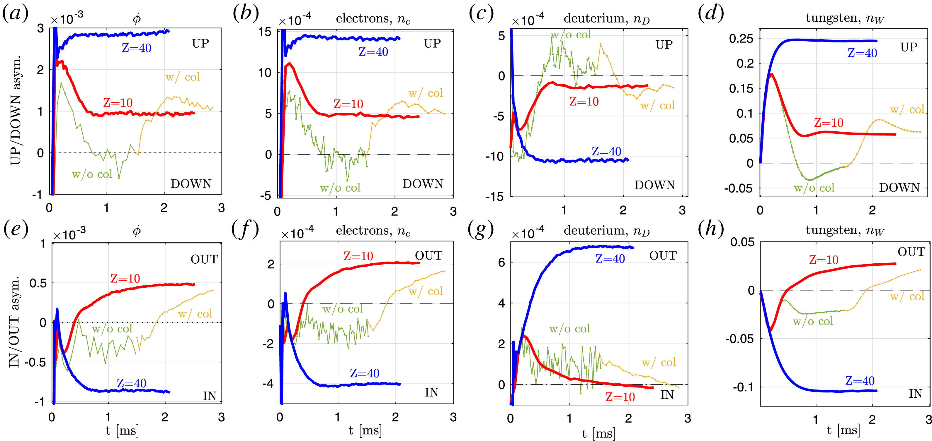
Poloidal asymmetry of large amplitude, $\unicode[STIX]{x1D6FF}n/\langle n\rangle \simeq 40\,\%$ , is observed for the highly collisional tungsten with $Z=40$ in figure 5. When we decrease the tungsten’s electric charge from $Z=40$ to $Z=10$ , we observe that the up/down asymmetry decreases by a factor ${\sim}5$ , as shown in figure 5(a). To assess the convergence of these asymmetry measurements, their time evolution is plotted in figure 11 of the appendix B. The up–down asymmetry plotted in figures 5 and 11 are measured with an estimate defined by

(5.1) $$\begin{eqnarray}\displaystyle & \displaystyle \unicode[STIX]{x1D6F6}_{w}=\frac{1}{{\mathcal{N}}}\oint \,\text{d}\unicode[STIX]{x1D703}\,\unicode[STIX]{x1D70E}\,(n_{w}-\langle n_{w}\rangle )/\langle n_{w}\rangle , & \displaystyle\end{eqnarray}$$

with $\unicode[STIX]{x1D70E}=+1$ on the upper part of the poloidal plane and $\unicode[STIX]{x1D70E}=-1$ on its lower part. The normalization factor is set to ${\mathcal{N}}=\oint \,\text{d}\unicode[STIX]{x1D703}\,\unicode[STIX]{x1D70E}\,\sin \unicode[STIX]{x1D703}\simeq 0.64$ . Formally, the asymmetry of a field ${\mathcal{A}}$ is measured by $\unicode[STIX]{x1D6F6}[\unicode[STIX]{x1D70E},{\mathcal{A}}](t)=\oint \,\text{d}\unicode[STIX]{x1D703}\,(\unicode[STIX]{x1D70E}\,{\mathcal{A}}(t)-\langle {\mathcal{A}}(t)\rangle )/|\langle {\mathcal{A}}(t)\rangle |/{\mathcal{N}}$ where one uses $\unicode[STIX]{x1D70E}=H(z-z_{\text{axis}})-H(z_{\text{axis}}-z)$ to measure the up–down asymmetry and $\unicode[STIX]{x1D70E}=H(r-r_{\text{axis}})-H(r_{\text{axis}}-r)$ to measure the in–out asymmetry; $H$ is the Heaviside step function, $r$ is the horizontal position, $z$ is the vertical position and $(r_{\text{axis}},z_{\text{axis}})$ is the position of the magnetic axis.

Figure 5.

Up–down (a) and in–out (b) asymmetries of the electrostatic potential(black), the electron density (blue), the main deuterium ion (red) and the tungsten impurity (green) are measured with (5.1). Tungsten asymmetries measurement are divided by $100$ to fit in the plot, but we remind the reader that tungsten represents $1/100$ of the electron charge, such that $0.01\unicode[STIX]{x1D6F6}_{w}\simeq \unicode[STIX]{x1D6F6}_{e}-0.99\unicode[STIX]{x1D6F6}_{D}$ as one can verify on this figure. Each panel contains the measurement for three simulations reported on the $x$ -axis: pure plasma, the impure plasma with tungsten $Z=10$ and the impure plasma with tungsten $Z=40$ . Measurements are made at surface $\unicode[STIX]{x1D713}_{n}=0.45$ .

Figure 5 clearly shows that the presence of tungsten impurities triggers the formation of asymmetries. Moreover, the up/down asymmetries have a significantly larger amplitude than the in/out asymmetries. Note that we verified, that $Z=40$ tungsten asymmetries with the same orientation and similar relative amplitude ( $\unicode[STIX]{x1D6FF}n_{w}/n_{w}$ ) are observed in a simulation with $400$ times less tungsten, i.e. $n_{w}=0.01\,n_{e}/Z/400=2.5^{-5}n_{e}/Z$ .

In/out asymmetries are weaker than up/down ones, but it is interesting to see that they are significantly different between $Z=10$ and $Z=40$ . Indeed, the tungsten asymmetries are of opposite phase in these two cases. When $Z=10$ the tungsten weakly accumulates outwardly, whereas when $Z=40$ tungsten more significantly accumulates inwardly. The weak outward accumulation of tungsten in the $Z=10$ case is likely the consequence of the weak plasma rotation and the corresponding centrifugal force (no source of rotation is imposed in our plasma, but the kinetic energy in the tungsten rotation is ${\sim}10\,\%$ of the tungsten thermal energy). Electrons are then neutralizing the tungsten charge asymmetry and their adiabatic response explains the potential asymmetry. On the other hand, in the plasma with tungsten $Z=40$ , the friction force between tungsten and the main ions are so strong that it overpowers the centrifugal force, as we will show in § 6. In this case, the friction force dominates and the in–out asymmetry does not have to follow the centrifugal force direction.

Moreover, in the plasma with tungsten $Z=40$ , the effect from tungsten charge density is so strong that both deuterium and electron species respond almost adiabatically (see figure 9), thus explaining their in/out asymmetry being opposite to that of the tungsten. In particular, the deuterium up/down asymmetry is larger by a factor ${\sim}10$ when $Z=40$ compared to when $Z=10$ , which is interesting because when $Z=40$ , the density of tungsten is $4$ times smaller but its effect on the deuterium up/down asymmetry is $10$ times bigger.

The fact that deuterium and electron particles require a stronger adiabatic response to neutralize the large amplitude asymmetry of collisional tungsten particles is interesting, because it suggests that the high- $Z$ tungsten could interact with both electron and ion non-adiabatic responses to the turbulent electrostatic fluctuations. This study is left for a future investigation.

Figure 6.

Neoclassical fluxes of particles (a–c) and energy (d–f) measured at the peak of the gradient. The plasma contains tungsten which charge represents $1\,\%$ of the electron charge. Results obtained using a linearization of the distribution function $f=f_{0}+\unicode[STIX]{x1D716}f_{1}$ are in black with dot markers and results obtained with XGCa are in colour with circle markers. Diagnostics are measured at $\unicode[STIX]{x1D713}_{n}=0.45$ where the gradients are peaked.

These big amplitude asymmetries of tungsten density have a strong impact on the tungsten fluxes (Angioni & Helander Reference Angioni and Helander2014) and must be properly resolved to calculate the neoclassical transport. To highlight the importance of solving the large amplitude asymmetries, we carried out NEO (Belli & Candy Reference Belli and Candy2008, Reference Belli and Candy2012) simulations that utilize linearization of the distribution function $f\simeq f_{0}+\unicode[STIX]{x1D716}f_{1}$ with the small $\unicode[STIX]{x1D716}$ assumption, where $f_{0}$ is a flux function. As expected, the results obtained from the linearized code disagree with the total-f XGCa results when large asymmetries develop; see the $Z=40$ simulation in figure 6. In comparison, when the asymmetries have small amplitudes $|{\tilde{n}}/\langle n\rangle |\lesssim 10\,\%$ the results obtained with the small ordering approximation are in good agreement with XGCa, showing less than $10\,\%$ difference in the $Z=10$ case. We find that when the collision frequency is high and the asymmetry is large ( $Z=40$ ), the local tungsten distribution function is nearly Maxwellian at all positions. There is essentially a shift in the $v_{\Vert }$ direction, $f\propto \exp (m(v_{\Vert }-U_{\Vert })^{2}/2T)$ .

The deuterium neoclassical fluxes can be affected by the presence of impurities through cross-species collisions or through the quasi-neutrality condition that enforces $\unicode[STIX]{x1D6E4}_{D}=\unicode[STIX]{x1D6E4}_{e}-Z_{W}\unicode[STIX]{x1D6E4}_{W}$ . Indeed, when the asymmetries are large and the tungsten particle flux is significant $|Z_{W}\unicode[STIX]{x1D6E4}_{W}/\unicode[STIX]{x1D6E4}_{e}|\simeq 1$ , the deuterium particle flux is significantly affected by the presence of impurities. In case with $Z=40$ , when tungsten asymmetries of large amplitude have developed, the tungsten particle flux is underestimated by the small ordering approximation $f(\unicode[STIX]{x1D713},\unicode[STIX]{x1D703})\simeq f_{0}(\unicode[STIX]{x1D713})+\unicode[STIX]{x1D716}f_{1}(\unicode[STIX]{x1D713},\unicode[STIX]{x1D703})$ and the main-ion particle flux is overestimated. We note here that, from figure 6(a–c), the ambipolar particle flux is roughly maintained between impurity ( $Z_{W}\unicode[STIX]{x1D6E4}_{W}$ ) and main ions ( $\unicode[STIX]{x1D6E4}_{D}$ ) as usually assumed in analytic theories. However, the electron particle flux is not negligibly small in both NEO and XGCa. Let us also point out that we also verified that the $Z=40$ tungsten particle flux, caused by the friction on the main ions, is proportional to the tungsten density. For this purpose, we have run a simulation that uses a tungsten density $400$ times smaller than that of our reference test case, and we measured the tungsten particle flux to decreases by the same factor $400$ . In this particular case, the tungsten charge flux is so small that the main-ion (D) particle flux is not significantly affected by the tungsten. Finally, the electron fluxes are in good agreement between NEO and XGCa in figure 6(b,e), even for the simulation with $Z=40$ where a large tungsten poloidal asymmetry is present. It shows that, in our test case problem, the fluxes of electrons are not strongly affected by the presence of tungsten’s poloidal asymmetry (they respond adiabatically to this large poloidal asymmetry). The slight increase ( ${\sim}+20\,\%$ ) of the electron fluxes observed when increasing the charge from $Z=10$ to $Z=40$ is rather due to the stronger electron collisions with $Z=40$ tungsten than with $Z=10$ tungsten. Indeed, collisions of electrons with tungsten are proportional to $\unicode[STIX]{x1D708}_{e,w}\propto Z_{w}^{2}n_{w}$ such that in our scan, where we keep the tungsten charge density fixed ( $n_{w}=n_{e}/100/Z_{w}$ ), the collision $\unicode[STIX]{x1D708}_{e,w}$ will increase ‘proportionally’ with $Z_{w}$ .

6 Drive for asymmetries

Figure 7.

Components of the reduced parallel momentum equation (6.2), for a simulation with tungsten $Z=40$ , normalized in the following form: $\unicode[STIX]{x1D735}_{\Vert }\ln n=ZeE_{\Vert }/T+F_{\Vert }/nT+\text{residual}$ , where each term is in units of $\text{m}^{-1}$ . The residual is the remaining part of the density gradient not driven by the electric field and friction force.

The physics of asymmetry formation can be understood from the parallel momentum equation

(6.1) $$\begin{eqnarray}\displaystyle & \displaystyle m_{a}n_{a}{\displaystyle \frac{\text{d}U_{\Vert ,a}}{\text{d}t}}=-\unicode[STIX]{x1D735}_{\Vert }p_{a}-\boldsymbol{b}\boldsymbol{\cdot }\unicode[STIX]{x1D735}\boldsymbol{\cdot }\unicode[STIX]{x03C0}_{a}+e_{a}n_{a}E_{\Vert }+F_{\Vert ,a}, & \displaystyle\end{eqnarray}$$

with the fluid moments defined in appendix A. In our case, the parallel friction force $F_{\Vert }$ is found to be the drive for the large poloidal asymmetry of tungsten with $Z=40$ , as shown in figure 7. This is in agreement with Helander (Reference Helander1998), where it was shown that in the case where the main ions are in the banana regime and the impurities are in the Pfirsch–Schlüter regime, the parallel viscous force can be neglected and the parallel momentum equation for tungsten reduces to, with a small residual term,

(6.2) $$\begin{eqnarray}\displaystyle & \displaystyle \unicode[STIX]{x1D735}_{\Vert }\ln n_{w}=eZE_{\Vert }/T_{w}+F_{\Vert ,w}/n_{w}T_{w}\quad (+\text{residual}), & \displaystyle\end{eqnarray}$$

where ‘residual’ represents the rest of the terms in equation (6.1) and is mostly from the parallel viscous force in a near steady state. From the XGCa simulation data, we can verify this reduced equation and gain more insight into the physics at play.

Figure 8.

Drive of density asymmetry on the surface $\unicode[STIX]{x1D713}_{n}=0.45$ along the poloidal direction $\unicode[STIX]{x1D703}$ , for three simulations: impure plasma with tungsten $Z=40$ (first column), impure plasma with tungsten $Z=10$ (second column) and pure plasma (last column). In each panel, the different components of the species parallel momentum equation (6.2) are shown; parallel friction force in blue, parallel electric field in red, parallel density gradient in green and residual containing the parallel viscous force in black. For comparison purpose, we ploted with a grey line in (a) (resp. (c)) the residual from the subplot (b) (resp. d) and (e)): it shows that the parallel viscosity is changing weakly between these different simulations.

The different components of (6.2) that drive the species density asymmetry on the surface $\unicode[STIX]{x1D713}_{n}=0.45$ are plotted in figure 8 for each species of the three different simulations. Results for the impure plasma simulation with tungsten $Z=40$ are in the first column (left); results with tungsten $Z=10$ are in the second column (middle); and the results of the pure plasma simulation are in the third column (right). The parallel momentum equation (6.2) is analysed for each species separately: tungsten results are in the first row, the deuterium results are in the second row and the electron results are in the last row. For example, (a) contains the different terms of the tungsten parallel momentum equation (6.2) obtained from the XGCa simulation with tungsten impurity at $Z=40$ , and (c) contains the terms of  (6.2) for deuterium in the same impure simulation.

It clearly appears, in the last row of figure 8, that electrons always respond adiabatically to the parallel electric field and that other terms contributing to the asymmetry are mainly negligible. Indeed, the electric field term (red) is almost equal to the density gradient (green). It also appears that the amplitude of the parallel electric field asymmetry (red) increases with the asymmetry of the tungsten density. This can be understood by the fact that more electrons are needed to neutralize the bigger tungsten asymmetry. Therefore, with electrons having a strong adiabatic response, a strong asymmetry of the electrostatic potential develops.

Figure 9.

Deuterium’s parallel momentum equation. More particularly, the contribution of each term of (6.2) to the deuterium parallel density gradient. Each component’s contribution is estimated by its correlation (6.3) with the deuterium parallel gradient $L_{\Vert ,d}^{-1}=\unicode[STIX]{x1D735}_{\Vert }n_{d}/n_{d}$ . Simulations of (a) pure plasma, (b) impure plasma with tungsten $Z=10$ and (c) impure plasma with tungsten $Z=40$ . Diagnostics made at surface $\unicode[STIX]{x1D713}_{n}=0.45$ with data of figure 8(c–e).

A consequence of the increase of the parallel electric field is that the deuterium asymmetry is then dominated by its adiabatic response to the parallel electric field in the impure plasma with tungsten $Z=40$ (figure 8 c) rather than by the parallel viscous force in the pure plasma (figure 8 e). In (c), the electric field term (red) is almost equal to the density gradient (green), whereas in (e) the residual containing the parallel viscous force (black) is almost equal to the density gradient (green). This increase of the adiabatic response further causes a reversal of the deuterium asymmetries, from an accumulation at the top in the pure plasma simulation to an accumulation at the bottom in the impure plasma with tungsten $Z=40$ , as shown in figure 5(a). In the case of the impure plasma with $Z=10$ the parallel electric field and the parallel viscous force nearly cancel each other in the deuterium parallel momentum equation (d), such that the deuterium asymmetry is weak for this value of $Z$ , as previously shown in figure 5.

This increase of the adiabatic response of deuterium associated with a reversal of the deuterium density asymmetry is illustrated in figure 9, where we plot the correlation

(6.3) $$\begin{eqnarray}\displaystyle & \displaystyle \text{corr}[{\mathcal{A}},L_{\Vert }^{-1}]={\displaystyle \frac{\displaystyle \int \,\text{d}\unicode[STIX]{x1D703}\,{\mathcal{A}}(\unicode[STIX]{x1D703})\,L_{\Vert }^{-1}(\unicode[STIX]{x1D703})}{\displaystyle \int \,\text{d}\unicode[STIX]{x1D703}\,L_{\Vert }^{-1}(\unicode[STIX]{x1D703})\,L_{\Vert }^{-1}(\unicode[STIX]{x1D703})}}, & \displaystyle\end{eqnarray}$$

between the parallel gradient $L_{\Vert }^{-1}=\unicode[STIX]{x1D735}_{\Vert }n/n$ and each term ( ${\mathcal{A}}$ ) on the right-hand side of (6.2). In the case of the pure plasma in (a), the deuterium asymmetry is driven by the residual, as shown by its positive correlation with the parallel deuterium density gradient $L_{\Vert ,D}^{-1}$ . The parallel electric field term is anti-correlated to $L_{\Vert ,D}^{-1}$ for this pure plasma. In comparison, for plasmas containing tungsten impurities, the deuterium asymmetry is driven by the parallel electric field, as shown by its positive correlation with $L_{\Vert ,D}^{-1}$ plotted in (b,c), where corr $[eZE_{\Vert }/T,L_{\Vert }^{-1}]\simeq 2$ with $Z=10$ and $\simeq 1$ with $Z=40$ , respectively. The correlation converging towards unity proves that the response of deuterium is mainly adiabatic when $Z=40$ .

Finally, we can see that the tungsten density asymmetry is driven by the parallel friction force when $Z=40$ (figure 8 a) and by the parallel viscous force when $Z=10$ (figure 8 b). With the highly collisional tungsten ( $Z=40$ ), we can even further narrow down the parallel momentum equation to be, at leading order,

(6.4) $$\begin{eqnarray}\displaystyle & \displaystyle \unicode[STIX]{x1D735}_{\Vert }\ln n_{w}\simeq F_{\Vert ,w}/nT_{w}. & \displaystyle\end{eqnarray}$$

This observation is confirmed in figure 10 where we compute the correlations between the terms on the right-hand side of the parallel momentum equation (6.2) with the tungsten parallel gradient term ( $L_{\Vert ,w}^{-1}=\unicode[STIX]{x1D735}_{\Vert }n_{w}/n_{w}$ ) on the left-hand side. Given that the tungsten collisionality is at banana plateau level for $Z=10$ and at Pfirsch–Schlüter level for $Z=40$ , this shows the transition from a low collisional regime where the tungsten asymmetries are driven by the parallel viscous force towards a high collisional regime where the tungsten asymmetries are driven by the parallel friction, as predicted by Helander (Reference Helander1998). See collision frequencies plotted in figure 2.

Figure 10.

Tungsten’s parallel momentum equation. More particularly, the contribution of each term of (6.2) to the tungsten parallel density gradient. Same calculation than in figure 10 but for tungsten. (a,b) Show the results from the impure plasma simulations with (a) tungsten $Z=10$ and (b) tungsten $Z=40$ . Diagnostics made at surface $\unicode[STIX]{x1D713}_{n}=0.45$ with data of figure 8(a,b).