R2. The map

The theory used as the foundation for the BOB map – discrete choice – is extremely broad (Ben-Akiva et al. Reference Ben-Akiva, de Palma, McFadden, Abou-Zeid, Chiappori, de Lapparent, Durlauf, Fosgerau, Fukuda, Hess, Manski, Pakes, Picard and Walker2012), and the map is a tool to help behavioral scientists navigate the large research terrain of its many applications. The map is intended to facilitate interdisciplinary communication and insights across different phenomena and different scales of analysis, from big-data statistics to qualitative observation at the individual scale. As Ruths & Shultz put it, the problem is highly dimensional, and the BOB map provides a framework on which future work can productively build. Spurrett takes us to task for fuzzy definitions of transparency and payoffs, but we think this flexibility is necessary to get people to use it as a basis for interdisciplinary communication and big-picture research, along the way making their own adaptations and modifications. To communicate with a business audience or public policymakers, for example, the north–south axis might be presented as extending from few choices in the north to many overwhelming choices in the south. Alternatively, as Buck advocates, the north–south axis might instead extend from “rational” to “emotional,” whereas in discrete-choice economics it would be called the “intensity of choice.” As we specify below, it all corresponds to closely related formulations mathematically.

These different shades of interpretation may provide multiple proxies to be measured in big data, which Godzińska & Wróbel rightly call for. For it the map to be applicable to decision making, anywhere from prehistory to the era of big data, we need a minimalist structure that allows for added elements such as emotions collected through surveys or text mining, different concepts of time, kinship or other cultural constructions recorded in anthropology, or the millennia of material culture in the archaeological record. Consider the vast range of scales from the population-level patterns in big-data studies of language use in online social media to the activity within individual brains. The spirit of our map is to use big data to generate hypotheses that are then tested by other means (including qualitative) at the individual/group level, which Godzińska & Wróbel invite us to consider, or even the level of neurobiology discussed by O'Donnell et al. We agree with Le Mens and with Roesch et al. that future uses of big data will include more sensitive measurements and more varied sources of information as the brain–computer interface develops. The BOB map provides a means of bridging scales of time and population. As Keane & Gerow and Roesch et al. point out, big-data literature puts a microscope on individuals but often underplays the complex distributional effects and dynamics that are visible at this large scale but also require a time depth.

Ross misunderstood us when he stated that we were relegating all economics to the northwest quadrant; we were putting only Homo economicus there. We actually see most of behavioral economics as lying just east of the northwest quadrant. Nevertheless, while we were careful not to map whole disciplines or individual researchers into the quadrants, we recognize that the bulk of literature in any one (sub)discipline tends to gravitate toward one of the quadrants.

Godzińska & Wróbel also see the map as too simplified to capture the essence of decision making, but most commentators accepted our invitation to fill in the map. The engagement of responders and the diversity of proposals to adapt the map help justify its simplicity, as Durlauf and MacCoun discuss. Even if a more complicated shape, such as the globe or tetrahedron suggested by Bookstein, could better capture certain interrelations, the cost would be the interdisciplinary common ground, and few in the BBS community would adopt these more complicated heuristic models. Furthermore, a more complicated geometry might make things worse by assuming too much. In other words, Bookstein rightly reminds us that “the map is not the territory.” We agree; the simple geometry is deliberate so that few would make this mistake. The simple two-dimensional form invites others to apply it or even modify it to suit their interests.

Together with Bookstein, Zhou et al. and Godzińska & Wróbel object to the “structuralist” dichotomy we have implied by the orthogonal axes, maintaining that transparency itself is socially influenced. Reader & Leris usefully caution against treating payoff transparency as a single entity, reminding us that transparency and the costs of decision making likely determine whether social or individual information is used. Zhou et al. present survey results in which social influence correlates with payoff transparency. We do not dispute either that b _t and J _t may correlate, or that in discrete-choice theory covariates that go into determining social influence and payoff transparency may indeed be correlated. We doubt, however, that the correlation will be the same in all cases, and one can easily envision situations where the two are anti-correlated or uncorrelated. Rather than assume some fixed correlation, the map is intended to represent how these shifts in decision making happen in any possible direction rather than just on fixed diagonals of assumed covariance.

R3. The terrain

Several commentators contributed useful ways forward in mapping the terrain of the map in more detail. This could be through measurement – such as sophisticated data extraction (Moat et al.) or subtle changes in distributions (Keane & Gerow) – or through multistage decision models (Analytis et al.; Hopfensitz et al.; McCain & Hamilton), or through the remarkably simple addition of “contour lines” (Christen & Brugger). We see the computer simulation by Analytis et al. as consistent with the predictions of our map: We just need to reverse the columns of their figure such that their “popularity-cue heuristic” model and its associated uniform distributions is in the west and their “popularity-set heuristic” model is in the east. In their two-stage decision model, each agent first eliminates the majority (e.g., 90%) of options. Agents following the popularity-set heuristic then choose among the shortlisted items through social influence, with probability proportional to popularity. This leads to just the kind of right-skewed distributions that we would expect in the east. Because agents choose the best from among only a 10% random sample, rather than from among all samples, the popularity-cue heuristic yields a more uniform distribution, consistent with the noisy southwest. In other words, the shortlisting stage of the popularity-cue heuristic is random selection, that is, pure southwest (b = 0).

Similarly, any social influence under the popularity-cue heuristic is fairly weak because it is activated only after shortlisting and only as a “fourth attribute” among three other attributes that remain reflective of quality. This repeated 10% random-sampling process weakens the tracking of quality, and as a result, the popularity of choices increases slowly in the direction toward the item of highest quality (from 0 to 100). Referring to the concern of Roesch et al. about rate of change, the popularity cue may only gradually sort out the best choices from the worst. Perhaps after more time steps, the gradient would be steeper from the worst to best (item 1 to item 100). We might therefore categorize the popularity-cue heuristic as being in the southwest quadrant as a result of the random sampling in step one, but in the northeast quarter of that quadrant because of the transparency (b > 0) and weak social influence in step two.

Like Analytis et al., who consider a two-stage process, Hopfensitz et al. also study games that have multiple stages. These games may be usefully studied in the extended BOB framework of our response here by modeling them as nested Logit Quantal response games where the first nest is the set of games one chooses to play in the first period, and the second nest is the set of strategies of the game chosen in the first period. The analog of (b, J) would be (b, J) for the choice of game in the first period and (b′, J′) for the second-period strategy choice of the game played in the second period. The choice of game in the first period includes the “game” of an “outside option” as in the commentary by Hopfensitz et al. Future research in multistage games proposed by Hopfensitz et al. is promising.

Similarly, McCain & Hamilton convince us that including social interactions and quantal responses at each stage is an exciting agenda for future research. McCain & Hamilton raise the interesting question of what happens if (b, J) vary across quadrants of the map in the context of anti-coordination games (Bramoullé Reference Bramoullé2007). Imagine there is a stoplight that has a large but finite penalty if you run a red light, and imagine their Drive On game being played by a pair of players with foggy glasses (a small b). When b = 0, each player plays “go” with probability 1/2 and plays “wait” with probability 1/2, and the probability of a crash is 1/4. But when b is infinite, the player facing a red light waits and traffic proceeds ideally.

We have emph1asized that the J _t parameter is an attempt to capture social influences, especially those types of influence that possess a “social multiplier” of policy relevance, which was stressed by Manski (Reference Manski1993) as being different from “spurious social effects” (Shalizi & Thomas Reference Shalizi and Thomas2010). Like Mesoudi and Le Mens, Ruths & Shultz are unsatisfied with the way we lump together all social-learning biases into the east. The map does, however, roughly cover the intensity of social tie tracked along the north–south dimension in the east. This makes it relevant to Granovetter's (Reference Granovetter1973) strong versus weak social ties and how the strength of these ties correlates with emotional closeness (e.g., Hill & Dunbar Reference Hill and Dunbar2003) – issues to which O'Donnell et al. refer. Hence, the north–south dimension does distinguish between the adaptive ratchet in the northeast, where social learning adaptively focuses on the most useful role models, and unbiased imitation in the southeast.

The Arab Spring, mentioned by Roesch et al. and O'Donnell et al. may be an example of the ambiguity of the effect of social media. When Gladwell (Reference Gladwell2010) pointed out “why the revolution will not be tweeted” – coincidentally just weeks before the Arab Spring uprising – he meant that revolutions require the strong social influence of the northeast, such as face-to-face interaction, rather than the weak ties of social media in the southeast. Social media are good for retrieving stolen cell phones left in cabs but not for carrying out revolutions, the success of which relies on organized hierarchy, not on here-today-gone-tomorrow social networks.

We are very aware that, as Ruths & Shultz point out, sigmoidal adoption curves may indicate social learning but that other models of independent learning (the simplest assuming a normal distribution of independent response times) can produce the same result (e.g., Bentley et al. Reference Bentley, Garnett and Brock2012; Brock & Durlauf Reference Brock and Durlauf2010; Hoppitt et al. Reference Hoppitt, Kandler, Kendal and Laland2010; Shultz Reference Shultz2003). This is why we propose distributions as a primary pattern for estimating J along the east–west axis of social influence. This tool can be refined, and we agree completely with Keane & Gerow that exploring the dynamics of how diagnostic popularity distributions change through time would refine the geography of our map within each quadrant. Fortunato et al. describe their insight from the precise popularity distribution of Wikipedia pages, and Keane & Gerow provide a nice example of how Zipf's Law in verb-phrase popularity became more “winner take all” among financial-media coverage as the stock-market crisis unfolded. Roesch et al. suggest that we could use “the velocity of change of decisions” and plot “vectors” on the map to show which way things are moving (vector direction) and at what rate (vector magnitude).

Although distributions are used to characterize the east–west axis, we agree with Analytis et al. that distributions may not be particularly diagnostic of transparency along the north–south axis. This is determined by the parameter b, which is sometimes called the “intensity of choice.” It measures the level of noisiness in choice – for example, when b = 0, noise in choice is so large that choice is completely random over the choice set. When b = ∞, transparency in the relative values of the payoffs to each choice is so high that there is no doubt whatsoever which choice yields the highest payoff. The intensity of choice, b _t , is a precise and useful way to model the concept of “transparency” at each date t, where (1) b _t  = 0 corresponds to the lowest level of transparency and the farthest south on our map, and (2) b _t  = ∞ corresponds to the highest level of transparency and the farthest north on our map. We realize that this modeling and conceptualization of “transparency” will not capture all useful interpretations, but we believe that it does capture a useful subset and makes a useful linkage to the very large and successful discrete-choice literature (Ben-Akiva et al. Reference Ben-Akiva, de Palma, McFadden, Abou-Zeid, Chiappori, de Lapparent, Durlauf, Fosgerau, Fukuda, Hess, Manski, Pakes, Picard and Walker2012).

The north–south axis (the b _t axis) is a useful way of looking at the gain in precision of predicting the future using big-data sets. Prediction requires an expectation by forward-looking agents, and this applies to social transparency, as we discuss below regarding the fascinating future of “looping,” to use the term of Christen & Brugger. By linking our approach to some classes of social interactions games, for instance, Hofensitz et al. suggest that the impact of social ties will be different in the north than in the south. We use their suggestions as an opportunity to explain the theory behind our Equation 1 of BOB, which lies in the domain of logistic quantal response games and quantal response (Nash) equilibria (McKelvey & Palfrey Reference McKelvey and Palfrey1995) and has been extended to include social interactions and covariates (Blume et al. Reference Blume, Brock, Durlauf, Ioannides, Benhabib, Jackson and Bisin2011; Brock & Durlauf Reference Brock and Durlauf2001a; Reference Brock, Durlauf, Blume and Durlauf2006). Let there be G groups with I players in each group. We can think of I as being a large number so that the law of large numbers gives a good approximation in what follows. Assume the groups are disjoint, that is, non-overlapping, for simplicity. As a stochastic best-reply function for player i at date t, consider the following modification of BOB's Equation 1 for a representative group g. The probability, P _itg (k), that player i in group g chooses k is then

where i, k, and g take the integer index values from 1 to I, N _t , and G, respectively. The expected value, ${{\bar{P}}^{e}_{itg}} \lpar k\rpar $ , denotes the belief, that is, the point expectation, that player i in group g holds on the average probability that k is chosen within his or her group.

Suppose point expectations are homogeneous for all players in all G groups – that is, assume 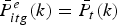${{\bar{P}}^{e}_{itg}} \lpar k\rpar = {{\bar{P}}_t}\lpar k\rpar $ . Then we have, further assuming that all covariate vectors are homogeneous across all players and all groups,

The fixed point $\bar{P}^* \lpar k\rpar = k$ of Equation 1.2, which we might consider a “norm” of collective behavior, has been more formally labeled as a “logistic quantal response equilibrium with social interactions” (Blume et al. Reference Blume, Brock, Durlauf, Ioannides, Benhabib, Jackson and Bisin2011; Brock & Durlauf Reference Brock, Durlauf, Heckman and Leamer2001b; Reference Brock, Durlauf, Blume and Durlauf2006; McKelvey & Palfrey Reference McKelvey and Palfrey1995). For example, say person i has both individual preferences concerning choice k and forward-looking expectations concerning the popularity of choice k. Combining these influences as ${a_k} + {c_k}^{\prime} {X_i} + {d_k}^{\prime} {{\bar X}_g} + {J_k}{{\bar{P}}_g}\lpar k\rpar $ , the probability that person i will choose item k is given by

In Equation 1.3, each player i has a covariate vector, X _i , and ${{\bar X}_g}$ denotes the average covariate vector averaged over players in i’s group g. A fixed point of Equation 1.3 is a generalization of Nash equilibrium for discrete-choice games, and multiple Nash equilibria may arise when b ≥ 0 and J _k  ≥ 0 for all k choices (Brock & Durlauf Reference Brock, Durlauf, Blume and Durlauf2006).

At the extreme north of our map, b = ∞, and there can be many fixed points when the Js are positive. A full analysis is beyond the scope of our response here (see Brock & Durlauf Reference Brock, Durlauf, Blume and Durlauf2006), but if we consider just the binary case, with N = 2 (Brock & Durlauf Reference Brock and Durlauf2001a), we can fully characterize the set of fixed points for the case J ₁  = J ₂  = J. For the case of non-negative social interactions, J ≥ 0, there can be three equilibria in many cases when bJ > 1 (e.g., in the northeast), if the difference among payoffs is not too large. MacCoun’s framework is similarly based on binary decisions; hence his “balance of pressures” (BOP) model and the BOB model apply to the kinds of tipping points and “voter” outcomes that MacCoun mentions, including threshold effects.

Another good representation of the north–south axis is “noise,” as suggested by Swain et al. with noise increasing as we move south. This noise dimension is what the social-physics literature of fairly deterministic “preferential attachment” network models has yet to engage with. As a case in point, Fortunato et al. argue that in a fully connected network, the random imitation of the southeast and popularity-based choice of the northeast (we actually map conformity in the equatorial east) are the same, through preferential attachment. But this neglects the greater degree of random noise as we move south, and hence the noise in choice popularity. Whereas the highly right-skewed distribution does not change much moving down the eastern edge of the map, as Analytis et al. also mention, the dynamics do change. This is the point of our Figure 2b.

To explore what happens with the greater noise in the south, let us examine equilibria for the extreme south, where b = 0. We have P(k) = 1/N, where N is the number of possible choices, that is, all players are just making choices at random, with the probability of each choice equal to 1/N. When we are in the deep south, where b approaches 0, we see that no matter how strong social ties are, that is, no matter how large J is, there is only one equilibrium. However, when we are in the extreme north, where b is very large, there will be, in many cases, three equilibria in the extreme northeast but only one equilibrium in the extreme northwest. In the extreme southeast, where J is very large, a small value of b can still satisfy bJ > 1, so multiple equilibria can easily occur.

R4. The future of big data

The southeast is where we find the unpredictability of success that Watts, Salganik, and colleagues have revealingly demonstrated over the years (e.g., Salganik et al. Reference Salganik, Dodds and Watts2006; Watts & Hasker Reference Watts and Hasker2006). This underlies our main question concerning big data: Will the popularity of crowd sourcing soon undo itself, decreasing b through information overload while simultaneously increasing social awareness of the crowd, J, and hence move online society toward the southeast? Slow movement of the key parameters (b,J) from west to east and from north to south, but especially from northwest to southeast, can easily produce behavior such as bifurcations and phase transitions, as unique equilibria morph into multiple equilibria (Berry et al. Reference Berry, Levinsohn and Pakes1995; Brock & Durlauf Reference Brock and Durlauf2001a; Reference Brock, Durlauf, Blume and Durlauf2006). Hence, Moat et al., who describe remarkable discoveries of the predictive nature of big data, may soon need to consider future increases in social-interaction effects as those predictive methods become commonplace.

We are grateful to Christen & Brugger for contributing a historical perspective through their invocation of Hacking's (Reference Hacking1992; Reference Hacking, Sperber, Premack and Premack1995) principle of “looping,” in which the identification of a phenomenon then feeds into the phenomenon itself. This is exactly why we believe that as predictive as big data might be at the moment, as soon as everyone becomes aware of these predictive algorithms, the competition to outpredict your competitor – whether in fashion, business, or the like – will tend to increase the unpredictability, much like what we see in the stock market. For example, whereas natural systems tend to exhibit early warning systems before critical transitions, financial systems are much more elusive (Scheffer et al. Reference Scheffer, Carpenter, Lenton, Bascompte, Brock, Dakos, van der Koppel, van de Leemput, Levin, van Nes, Pascual and Vandermeer2012).

Fan & Suchow propose that self-awareness can lead a group to seek out new knowledge and reposition itself on the map. They propose that motivation to solve a problem is a key variable driving groups northward on the map. We are not sure that the crowd can guide its own trajectory, however. We all seek to head north, but as Schmidt points out, the onslaught of big data may break lots of compasses, given that practically any opinion on any issue from climate change to genetically modified foods to measles vaccines and evolution can be found online. As Schmidt points out, even human identity becomes ambiguous as each person's digital shadow grows with multiple memberships, enrollments, sign-ups, connections, and so on. Intriguingly, Schmidt proposes that the southeast may subdue the data deluge “through a global relativity,” while at the same time making the problem worse through collective behaviors. Schmidt rightly asks whether any of us can be experts anymore, which poses the compelling question of what happens if we were to crowd-source all our decisions, as is already explored in current science fiction. Schmidt suggests this may already be happening in medicine, perhaps the most information-deluged science, where the diagnosis of newly named syndromes has been rising dramatically in a way that is clustered in time and space, suggestive of the southeast.

As O'Donnell et al. point out, the neural systems for self-knowledge are involved in social cognition. In fact, Christen & Brugger add self-reflection to the list of suggested third dimensions to the map because social influence depends on the models people have of themselves and what drives their behavior (e.g., a conscious effort to be a nonconformist) and, of course, whether one is aware of this self-reflection (buck the nonconformist trend by being ironically conformist, for example). This looping can go on forever, reminiscent of what Yogi Berra once said about a popular Italian restaurant in St. Louis: “No one goes there anymore. It's too crowded.”

As agents compete to outpredict each other, we enter Mesoudi’s discussion of adaptive landscapes (see also Mesoudi Reference Mesoudi, O'Brien and Shennan2010; Mesoudi & O'Brien Reference Mesoudi and O'Brien2008a; Reference Mesoudi and O'Brien2008b). Anderson et al. (Reference Anderson, de Palma and Thisse1992) give us a formula for this:

which relates to ideas and techniques from entropy maximization in Bayesian statistics – tools from mean-field theory that allow us to approximate more complicated social networks, economics, and finance (Ben-Akiva et al. Reference Ben-Akiva, de Palma, McFadden, Abou-Zeid, Chiappori, de Lapparent, Durlauf, Fosgerau, Fukuda, Hess, Manski, Pakes, Picard and Walker2012; Brock Reference Brock1993; Hommes Reference Hommes2013). Note that as b _t  → ∞ from south to north, this landscape function converges to $U_{i^*},i^*=\arg\!\max_k\{U_k\}$ and hence the landscape of Equation 1.4 moves toward a spiked, or so-called “Mount Fuji,” shape on the space of choices, {1, 2, …, N _t }. In contrast, moving from west to east, as J _t increases, multiple equilibria become possible so the landscape becomes more “rugged,” and the potential for instability grows. Generally speaking, instabilities in collective dynamics will be north of the “equator,” and the northeast especially is where instabilities and emergent bifurcations could link to studies of early warning signals (Scheffer et al. Reference Scheffer, Carpenter, Lenton, Bascompte, Brock, Dakos, van der Koppel, van de Leemput, Levin, van Nes, Pascual and Vandermeer2012).

Roesch et al. mention the “exponential velocity” of change with access to new technology, but we need to be careful about tempo versus mode of change, which might lead us to ask whether the current rate of change is any more “exponential” than in the early twentieth century, with most technologies taking off in the same sigmoidal form (Bentley & O'Brien Reference Bentley and O'Brien2012; O'Brien & Bentley Reference O'Brien and Bentley2011). Rather than accelerating change, in some cases increasing access to crowd-sourced data may lead to stasis, especially if accurate popularity statistics are approached with a conformity bias.

On an adaptive fitness landscape, such as what Mesoudi describes, there are different ways to avoid getting stuck on a low peak when higher peaks are nearby. The most straightforward is a global view of the landscape from the authoritative vantage of a “control tower,” which is the beauty of the Sixth Sense Transport system that Norgate et al. have developed for mitigating traffic problems. Without this kind of top-down control, the other means is an optimal balance of information producers and information scroungers, as Mesoudi would describe it (see also Mesoudi Reference Mesoudi2008), or a balance of “exploration and exploitation,” in the more business-like language of Axelrod and Cohen (Reference Axelrod and Cohen1999).

On our map, this means an optimal, situation-specific balance of noise (the opposite of transparency) and social influence. Clearly, the balance is critical. Norgate et al. point out that “increased imitation can be desirable,” and Zhou et al. note that when people have little knowledge on which to base their decisions, it is helpful to imitate the successful judgments, or to average the judgments, of others. But under a deluge of information, imitation might also bring about the kind of “pluralistic ignorance” that Christen & Brugger suggest could stabilize social dynamics in a suboptimal state. Crowd-sourcing may even preserve an undesirable status quo. As Uhlmann & Silberzahn discuss, we assume that the best person for the job gets hired – the northwest – but actual online hiring decisions tend to drift southeast, as information overload leads employers to rely on gender stereotypes as a shortcut decision strategy.

As a result, noise can be a means of (unintentionally) exploring the landscape, as nicely shown by Hopfensitz et al. with their game involving ambiguous payoffs (less-transparent payoffs in our language) and strong social interactions, which can yield a more efficient outcome than the same game with less of those aspects in the north. Noise in the dynamics of the game can lead to coordination equilibrium with a higher level of social welfare when multiple Nash equilibria are present in coordination games (Kandori et al. Reference Kandori, Mailath and Rob1993). Hopfensitz et al. formulate their first game so that each player who has ties to another player chooses his or her strategy to maximize a combined utility that is a weighted sum of his own selfish interest and the joint interest of the two players. If the function U in BOB's Equation 1 is replaced by the Hofensitz et al. function, and b = 0, then the players will choose their strategies randomly with equal probability, and yet, as Hopfensitz et al. point out, this may yield a higher average welfare than in the case where b is large.

O'Donnell et al. and Pfister & Böhm both object to the idea of “independence” as a possibility for human beings, whose minds are social, even when physically alone. They point to neuroimaging studies that show humans are prone to adopt ideas that they may think are becoming more popular (see also Berger & Le Mens Reference Berger and Le Mens2009; Berger & Milkman Reference Berger and Milkman2012; Gureckis & Goldstone Reference Gureckis and Goldstone2009), even if they happen to be alone at the time. As O'Donnell et al. note, the neural systems for self-knowledge are involved in social cognition, and social inclusion versus rejection involves the same areas of the brain as physical pleasure and pain. As compelling as the evidence for the “social brain” may be, this is more of a semantic issue for us, to be plotted on the map using data at the scale of individuals or populations.

As Moat et al. correctly point out, we were not generous enough to the new big-data sciences of predicting near-future behavior based on recent past behavior. Roesch et al. and Moat et al. report on the incredible progress in data generation concerning individual behaviors correlated with all the other geolocated measures one can derive such as ambient temperature, noise level, luminance information, and energy consumption. Our review was only the tip of the iceberg in terms of big-data studies aimed at forecasting future behavior such as financial and commercial activity, economic trends, epidemics, and even crime. As behavioral scientists, we are in awe of the developments in e-commerce, such as recommendation systems in retail applications. As a clarification, we would see computer algorithms recommending products or services as probably qualifying as social influence, even if the recommendation algorithms are using social information to act on people who may be alone at their computers (an ambiguity raised by O'Donnell et al.).

Predicting the near future by extrapolating the recent past is a huge advantage of big data, especially because it does not require deep understanding of the causality behind behaviors in terms of decision making. Causality is enigmatic in the same way that social diffusion (northeast) can be so difficult to distinguish from (northwest) homophily (Aral et al. Reference Aral, Muchnik and Sundararajan2009), but for prediction and intervention, this may make little difference. The prescription is to intervene at the point of highest activity, with or without knowledge of its cause. Moat et al. make the important point that not only can big data assist in “predicting the present” (Choi & Varian Reference Choi and Varian2012), but it can also play a major role in predicting the future – for example, in the trading-strategy-returns studies that they cite.

Although our map is an extremely coarse-grained approximation of the highly dimensioned correlation and prediction studies that Moat et al. cite, we show here how the b _t index of “transparency” relates to those studies. Note that

In applications of discrete-choice theory to correlation and prediction, the Us are parameterized as functions of observable covariates and parameters and taken to datasets for hypothesis formulation, estimation of parameters, and testing of hypotheses. This activity includes correlation studies and prediction studies. If b _t  = 0, the differences in the estimated values of the Us give no information as to the observed frequencies of choices between choice k and choice N_t at date t. In this case, the covariates give no information on predicting the present or the future. More concretely in the Preis et al. (Reference Preis, Moat and Stanley2013) study that Moat et al. cite, we could think of big-data sets from Google Trends as a way of not only improving the specification of the Us in Equation 1.5, but also of increasing the size of b_t relative to previous studies.

To be sure, this may soon be less painstaking with better data and algorithms based on pioneering studies by Aral and Walker (Reference Aral and Walker2012) and others, at which point the map will be even more appropriate because measuring the east–west dimension might be routine. Mapping the nature of decisions is crucial because big data will soon be part of our decisions rather than an independent measure of them. Roesch et al. mention Project Glass (Google Inc. 2012) and the ubiquity of big data in daily activities, although we note that still only about a third of the world's population has Internet access. As the growing public familiarity with big-data patterns feeds into the decisions themselves (Christen & Brugger; Fan & Suchow; Schmidt), will big data still be as predictive (Moat et al.), or are we heading toward a situation, as with financial markets, where everyone is trying to outpredict everyone else? How will collective behavior change as we all become omniscient about global trends in those very behaviors? Buck is correct to discuss McLuhan's (Reference McLuhan1964) “medium is the message” philosophy, which underlies our basic question of how big data will change behavior and not merely record it objectively.

In conclusion, we again want to thank all the commentators for providing us much more in the way of excellent proposals for modifying and extending the BOB map into areas that we could not have anticipated. Our only regret is not having the time and the space to respond to the comments in the terms they deserve. We hope both our target article and the accompanying commentaries will inspire other behavioral scientists with an interest in decision making to use the discussions as launching pads for their own work. We very much look forward to what those others have to say.