4.1. DNO-truncation models

Following the seminal work of Craig & Sulem (Reference Craig and Sulem1993), which builds on the canonical variables introduced by Zakharov (Reference Zakharov1972), the kinematic and dynamic boundary conditions (2.3) and (2.9) can be recast in terms of the velocity potential at the ice–water interface, defined as $\xi (x,y,t)=\phi (x,y,\eta ,t)$ , and the surface displacement $\eta$ . To begin, we introduce the Dirichlet–Neumann operator (DNO), which provides the normal velocity at the free surface, as follows:

(4.1) \begin{equation} G(\eta ,h)\xi =\big (\phi _z-\phi _x\eta _x-\phi _y\eta _y\big )_{z=\eta }. \end{equation}

It is clear that the kinematic boundary condition can be expressed succinctly as $\eta _t=G(\eta ,h)\xi$ . We suppress the dependence of $G$ on $\eta$ and $h$ for simplicity of notation hereafter. By using the DNO, we can subsequently rewrite the dynamic boundary condition as

(4.2) \begin{equation} \begin{aligned} \xi _t=&\;\frac {1}{2\big (1+|\boldsymbol{\nabla }\eta |^2\big )}\big [(G\xi )^2+2(G\xi )\left (\boldsymbol{\nabla }\eta \boldsymbol{\cdot }\boldsymbol{\nabla }\xi \right )-|\boldsymbol{\nabla }\xi |^2\big ]\\ &\;-\alpha (G\xi )_t-\beta G\xi -\gamma \Delta ^2G\xi -\eta -\frac {\delta E_b}{\delta \eta }+f, \end{aligned} \end{equation}

where $\varDelta$ is the horizontal Laplace operator defined as $\varDelta =\boldsymbol{\nabla }\boldsymbol{\cdot }\boldsymbol{\nabla}$ . This approach offers a significant simplification by reducing the 3-D nonlinear wave problem to a 2-D one that is defined solely at the free surface. It also eliminates the need to solve the Laplace equation throughout the entire fluid domain, thereby removing the dependence on the vertical coordinate $z$ .

Coifman & Meyer (Reference Coifman and Meyer1985) demonstrated that if both the $L^{\infty }$ -norm and the Lipschitz-norm of $\eta$ are less than a specified constant, then $G$ is an analytic function of $\eta$ . As a result, the DNO can be expressed as a Taylor series in $\eta$ , represented as $G=\varSigma _{j=0}^\infty G_{\!j}(\eta ,h)$ , where $G_{\!j}(\eta ,h)$ is homogeneous of degree $j$ in $\eta$ . Again, we omit the dependence of $G_{\!j}$ on $\eta$ and $h$ for brevity. For finite depth, the first three terms of the Taylor series are given by

(4.3) \begin{align} &G_0=|D|\text{tanh}(h|D|), \\[-12pt]\nonumber \end{align}

(4.4) \begin{align} &G_1=D\boldsymbol{\cdot }\eta D-G_0\eta G_0, \\[-12pt]\nonumber \end{align}

(4.5) \begin{align} &G_2=-\frac 12\big [G_0\eta ^2|D|^2+|D|^2\eta ^2G_0-2G_0\eta G_0\eta G_0\big], \end{align}

where $D=-\mathrm{i}\boldsymbol{\nabla}$ and $|D|=(-\varDelta )^{(1/2)}$ . In the case of infinite water depth, the leading-order operator $G_0=|D|$ , while the forms for $G_1$ and $G_2$ remain unchanged from their counterparts in the finite depth scenario. By substituting the expansion of $G$ into the boundary conditions and truncating all terms involving $\xi$ to cubic order, we obtain

(4.6) \begin{equation} \eta _t=\left (G_0+G_1+G_2\right )\xi \end{equation}

and

(4.7) \begin{align} M\xi _t=&\;\frac 12\big [(G_0\xi )^2-|\boldsymbol{\nabla }\xi |^2+2(G_0\xi )(G_1\xi )+2(G_0\xi )\left (\boldsymbol{\nabla }\eta \boldsymbol{\cdot }\boldsymbol{\nabla }\xi \right )\big] \nonumber\\ &\;-\eta +\alpha \left [\boldsymbol{\nabla }\boldsymbol{\cdot }\left (G_0\xi +G_1\xi \right )\boldsymbol{\nabla }\xi +G_0\left (G_0\xi +G_1\xi \right )G_0\xi \right ] \nonumber\\ &\;-\alpha \big [G_0\left (G_0\xi \right )\left (\eta \Delta \xi +G_0\eta G_0\xi \right )+\Delta \eta \left (G_0\xi \right )^2+G_0\eta G_0\left (G_0\xi \right )^2\big] \nonumber\\ &\;-\big (\beta +\gamma \Delta ^2\big )\left (G_0+G_1+G_2\right )\xi -\frac {\delta E_b}{\delta \eta }+f, \end{align}

where $M=1+\alpha (G_0+G_1+G_2)$ is a pseudo-differential operator. For numerical convenience, both sides of (4.7) are multiplied by the inverse operator $M^{-1}$ , which can be formally expanded as

(4.8) \begin{equation} M^{-1}=K^{-1}-\alpha K^{-1}(G_1+G_2)K^{-1}+\alpha ^2K^{-1}G_1K^{-1}G_1K^{-1}+{\cdots}, \end{equation}

where $K=1+\alpha G_0$ . For ease of notation, we define

(4.9) \begin{align} M_0=K^{-1},\quad M_1=-\alpha K^{-1}G_1K^{-1},\quad M_2=-\alpha K^{-1}\big (G_2-\alpha G_1K^{-1}G_1\big )K^{-1} \end{align}

Substituting the expansion of $M$ into the dynamic boundary condition (4.7) ultimately yields

(4.10) \begin{align} \begin{aligned} \xi _t=&\;M_0(G_0\xi )\left (G_1\xi +\boldsymbol{\nabla }\eta \boldsymbol{\cdot }\boldsymbol{\nabla }\xi \right )+\frac 12(M_0+M_1)\big [(G_0\xi )^2-|\boldsymbol{\nabla }\xi |^2\big ]+\alpha (M_0\\ &\;+M_1)\big [\boldsymbol{\nabla }\boldsymbol{\cdot }(G_0\xi )\boldsymbol{\nabla }\xi +G_0(G_0\xi )^2\big]+\alpha M_0\left [\boldsymbol{\nabla }\boldsymbol{\cdot }(G_1\xi )\boldsymbol{\nabla }\xi +G_0(G_1\xi )(G_0\xi )\right ]\\ &\;-\alpha M_0\big [G_0(G_0\xi )(\eta \Delta \xi +G_0\eta G_0\xi )+\Delta \eta (G_0\xi )^2+G_0\eta G_0(G_0\xi )^2\big ]\\ &\;-M_0\big (\beta +\gamma \Delta ^2\big )(G_0+G_1+G_2)\xi -M_1\big (\beta +\gamma \Delta ^2\big )(G_0+G_1)\xi \\ &\;-M_2\big (\beta +\gamma \Delta ^2\big )G_0\xi -(M_0+M_1+M_2)\left (\eta +\frac {\delta E_b}{\delta \eta }-f\right )\!. \end{aligned} \end{align}

From a mathematical perspective, further approximating the inverse operator $M^{-1}$ disrupts the complete retention of effects stemming from gravity, elasticity and moving force, as described in (4.7). However, this trade-off is acceptable for numerical computations, where prioritising tractability and efficiency is essential. It is also emphasised that, unlike typical weakly nonlinear models, (4.7) accurately preserves the restoring force resulting from the nonlinear elastic bending effect. Within a doubly periodic domain, the coupled system described by (4.6) and (4.10) will now be referred to as the cubic DNO-truncation model. If we neglect the cubic nonlinear terms in (4.6) and (4.10), then the resultant system is termed the quadratic DNO-truncation model, which has been numerically studied by Dinvay et al. (Reference Dinvay, Kalisch and Părău2019) with a linear elastic bending term.

These two fully dispersive models can be efficiently computed using a pseudo-spectral method for spatial discretisation, calculating all derivatives in Fourier space with spectral accuracy, while computing nonlinear terms pseudospectrally in real space. Time integration of the system is performed using a classic fourth-order Runge–Kutta method. To compute a free solitary wave when the viscous effects are neglected, we first calculate forced hydroelastic waves using the Newton–Raphson method. The external pressure is then gradually diminished while maintaining a constant wave amplitude. The resulting solution serves as an initial guess for subsequent computations in the unforced system. All the computations are de-aliased with a doubling of Fourier modes and no filters are used. For solitary waves of wavepacket type, small-amplitude solutions often present significant challenges in terms of accurate computation due to their slower spatial decay. Consequently, it is necessary to gradually expand the computational domain as the amplitude decreases (or equivalently, the solutions approach the bifurcation point).

4.2. A normal form analysis

The nonlinear Schrödinger (NLS) equation is a universal model widely used across various scientific fields, providing a standard description of the evolution of the envelope of dispersive and/or diffracting quasi-monochromatic, plane, weakly nonlinear waves. In the context of free-surface water waves, the envelope dynamics of a wave packet in the small-amplitude deep-water limit can be effectively approximated by a 2 + 1-dimensional cubic NLS equation. This equation is instrumental in predicting the Benjamin–Feir instability of wave trains and the existence of solitary wave packets. However, when conducting modulation analysis, the Benney–Roskes–Davey–Stewartson (BRDS) equation is derived for waves propagating in water of finite depth, which necessitates the inclusion of the induced mean flow (Benney & Roskes Reference Benney and Roskes1969). In this discussion, we will outline the derivation of the BRDS equation for small-amplitude hydroelastic waves, comparing the results from both the quadratic and cubic models.

Consider the hydroelastic wave problem in the absence of viscosity and externally applied pressure, which means that $\beta =\gamma =f=0$ in the dynamic boundary condition (2.15). For weakly nonlinear hydroelastic waves, we assume that $\eta \sim O(\epsilon )$ and $\phi \sim O(\epsilon )$ , where $\epsilon$ is a small parameter used to measure wave steepness. Consequently, the velocity potential function at the free surface can be expanded about $z=0$ as

(4.11) \begin{equation} \phi (x,y,\eta ,t)=\phi (x,y,0,t)+\eta \phi _z(x,y,0,t)+\frac 12\eta ^2\phi _{zz}(x,y,0,t)+O(\epsilon ^4)\,. \end{equation}

This allows us to express the surface boundary conditions at $z=0$ up to the cubic order as

(4.12) \begin{equation} \phi _z-\eta _t=\phi _x\eta _x+\phi _y\eta _y-\eta \phi _{zz}+\eta \eta _x\phi _{xz}+\eta \eta _y\phi _{yz}-\frac 12\eta ^2\phi _{zzz} \end{equation}

and

(4.13) \begin{equation} \begin{aligned} \phi _t+\big (1+\Delta ^2\big )\eta &\;+\alpha \eta _{tt}=\eta \phi _{zt}-\frac 12\phi _x^2-\frac 12\phi _y^2-\frac 12\phi _z^2-\frac 12\eta ^2\phi _{zzt}-\eta \phi _x\phi _{xz}\\ &\;-\eta \phi _y\phi _{yz}-\eta \phi _z\phi _{zy}+\frac 52\eta ^2_x\eta _{xxxx}+\frac 52\eta ^3_{xx}+10\eta _x\eta _{xx}\eta _{xxx}\,. \end{aligned} \end{equation}

This text provides a brief outline of the derivation of the BRDS equation for hydroelastic waves and for those interested in more detailed information, please refer to Milewski & Wang (Reference Milewski and Wang2013). We consider the evolution of a wave packet whose slow dependence is comparable in both the $x$ - and $y$ -directions, while its rapid oscillations occurs solely in the $x$ -direction. This means the wave packet will propagate along the $x$ -direction, exhibiting a slowly evolving structure in both the $x$ - and $y$ -directions. To derive the governing equation for the wave envelope, we introduce the following slow variables: $X=\epsilon x$ , $Y=\epsilon y$ , $T=\epsilon t$ and $\tau =\epsilon ^2 t$ , and choose $e^{\mathrm{i}(kx-\omega t)}$ as the carrier wave. We then seek a solution of the form

(4.14) \begin{align} &\eta =\epsilon A(X-c_{\!g}T,Y,\tau )e^{\mathrm{i}\theta }+\sum _{n=2}^\infty \epsilon ^n\sum _{j=0}^nA_{nj}(X-c_{\!g}T,Y,\tau )e^{j\mathrm{i}\theta }+\mathrm{c.c.}, \\[-12pt]\nonumber \end{align}

(4.15) \begin{align} &\phi =\sum _{n=1}^\infty \epsilon ^n\sum _{j=0}^n\phi _{nj}(X-c_{\!g}T,Y,z,\tau )e^{j\mathrm{i}\theta }+\mathrm{c.c.}, \end{align}

where $\theta =kx-\omega t$ represents the phase of the carrier wave and ‘c.c.’ denotes the complex conjugate. By substituting the ansatzes (4.14) and (4.15) into (4.12) and (4.13), we can derive the linear dispersion relation at the leading order:

(4.16) \begin{equation} \omega ^2=\frac {k(1+k^4)\text{tanh}(\textit{kh})}{1+\alpha k\text{tanh}(\textit{kh})}. \end{equation}

At the order of $O(\epsilon ^2)$ , we obtain the expression for $c_{\!g}$ as

(4.17) \begin{equation} c_{\!g}=\frac {(1+5k^4-\alpha \omega ^2)\text{tanh}(\textit{kh})+kh(1+k^4-\alpha \omega ^2)\text{sech}^2(\textit{kh})}{2\omega (1+\alpha k\text{tanh}(\textit{kh}))}= \frac {\mathrm{d}\omega }{\mathrm{d}k}. \end{equation}

This indicates that $c_{\!g}$ represents the group velocity, justifying our choice of $c_{\!g}$ as the velocity of the wave packet. At $O(\epsilon ^3)$ , the solvability condition for eliminating the secular terms yields the following non-local BRDS equation:

(4.18) \begin{equation} \mathrm{i}A_{\tau }+\frac {\omega ^{\prime \prime }}{2}A_{\textit{XX}}+\frac {c_{\!g}}{2k}A_{\textit{YY}}+\lambda _1\widetilde {\Delta }^{-1}\left [|A|^2\right ]_{\textit{XX}}A+\lambda _2|A|^2A=0, \end{equation}

where $\widetilde {\Delta }=(1-h^{-1}c_{\!g}^2)\partial _{\textit{XX}}+\partial _{\textit{YY}}$ . The coefficients in (4.18) are given by

(4.19) \begin{equation} \lambda _1=\frac {1}{h\left [1+\alpha k\text{tanh}(\textit{kh})\right ]}\left [k+\frac {k\omega c_{\!g}}{2\sinh (\textit{kh})\cosh (\textit{kh})}\right ]\left [\frac {\omega ^2c_{\!g}}{\sinh ^2(\textit{kh})}+\frac {2\omega }{\text{tanh}(\textit{kh})}\right ] \end{equation}

and

(4.20) \begin{equation} \begin{aligned} \lambda _2=&\;\frac {\omega k^2}{1+\alpha k\text{tanh}(\textit{kh})}\left \{\frac {g_1(k)+12\alpha k(4k^4-1)\text{tanh}(\textit{kh})}{4\text{tanh}^2(\textit{kh})g_2(k)}\right .\\ &\;\left .+\frac 12\left [\frac {1+k^4}{\sinh ^2(\textit{kh})\cosh ^2(\textit{kh})}-4\right ]\right \}+\frac {5\omega k^6}{2(1+k^4)}, \end{aligned} \end{equation}

where

(4.21) \begin{align} &g_1(k)=\big (1+k^4\big )\big [\text{tanh}^4(\textit{kh})-10\text{tanh}^2(\textit{kh})+9\big]+60k^4, \\[-12pt]\nonumber \end{align}

(4.22) \begin{align} &g_2(k)=15k^4+3\alpha k(4k^4-1)\text{tanh}(\textit{kh})-(1+k^4)\text{tanh}^2(\textit{kh}). \end{align}

If the inertia term is ignored (i.e. $\alpha =0$ ), the coefficients align with those derived by Milewski & Wang (Reference Milewski and Wang2013). When the dependence on $Y$ becomes negligible – essentially reducing the problem to one horizontal dimension – the BRDS equation simplifies to the classical 1 + 1-dimensional NLS equation:

(4.23) \begin{equation} \mathrm{i}A_\tau +\frac {\omega ''}{2}A_{\textit{XX}}+\left (\frac {\lambda _1}{1-h^{-1}c_{\!g}^2}+\lambda _2\right )|A|^2A=0\,, \end{equation}

consistent with the results of Meng & Wang (Reference Meng and Wang2022). In the case of infinite water depth, the contribution from mean flow in (4.18) disappears, resulting in

(4.24) \begin{equation} \lambda _1\sim \frac {2k\omega }{h(1+\alpha k)}\to 0\quad \text{as} \quad h\to \infty \,. \end{equation}

Consequently, the BRDS equation degenerates into the classical 2 + 1-dimensional NLS equation:

(4.25) \begin{equation} \mathrm{i}A_{\tau }+\frac {\omega ^{\prime \prime }}{2}A_{\textit{XX}}+\frac {c_{\!g}}{2k}A_{\textit{YY}}+\lambda _2|A|^2A=0\,. \end{equation}

Figure 2.

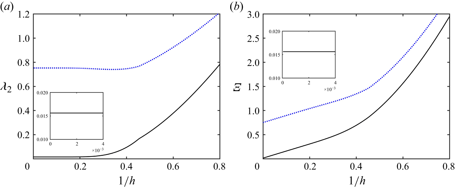
(a) $\lambda _2$ and (b) $\varXi$ versus $1/h$ . The blue dotted lines correspond to the quadratic model, while the black solid lines represent the cubic model. The physical parameters required for the calculations are detailed in the McMurdo Sound case in table 1.

It is important to emphasise that deriving the correct BRDS equation requires expanding the full Euler equations to cubic order. In fact, we can also obtain the BRDS equation from the quadratic DNO-truncation model, which is equivalent to neglecting the cubic nonlinear terms in (4.12) and (4.13). Since the governing equations of the quadratic model differ from those of the cubic model only at $O(\epsilon ^3)$ , the linear dispersion relation, the group velocity $c_{\!g}$ and $\lambda _1$ are identical for both models. However, the quadratic model is unable to capture the complete nonlinear interaction, resulting in an inaccurate coefficient $\lambda _2$ . We denote this coefficient as $\widetilde {\lambda }_2$ to distinguish it from that of the cubic model and express it as

(4.26) \begin{equation} \widetilde {\lambda }_2=\frac {\omega k^2}{1+\alpha k\text{tanh}(\textit{kh})}\left [\frac {g_1(k)+12\alpha k(4k^4-1)\text{tanh}(\textit{kh})}{4\text{tanh}^2(\textit{kh})g_2(k)}\right ]\!. \end{equation}

Our primary concern is the behaviour of hydroelastic waves as the load velocity approaches a critical point. At this point, the group and phase velocities are nearly equal to the load speed, leading to wave resonance and the periodic shedding of solitary wave packets (Milewski, Vanden-Broeck & Wang Reference Milewski, Vanden-Broeck and Wang2011). Consequently, distinguishing between the focusing and defocusing types of the BRDS equation is essential for understanding the wave dynamics at this juncture. At criticality, where the phase speed reaches its minimum value, both $c_{\!g}$ and $\omega ''$ are positive. Cipolatti (Reference Cipolatti1992) introduced a new parameter

(4.27) \begin{equation} \varXi =\frac {\lambda _1}{1-h^{-1}c_{\!g}^2}+\lambda _2, \end{equation}

and proved that $\varXi \gt 0$ is a sufficient condition for the equation to possess a localised ground state solitary wave. Henceforth, we will refer to the BRDS equation as the focusing type based on this criterion.

The inclusion of the inertial term leads to $\lambda _2\gt 0$ and $\varXi \gt 0$ for the cubic DNO-truncation model, making the equation focusing, as illustrated by black solid lines in figure 2. For comparison, we also display $\widetilde {\lambda }_2$ for the quadratic model in figure 2 using a blue dashed line. The notable difference in the nonlinear coefficient between the two models indicates that there will be substantial differences in the solutions regarding quantity, even though both models qualitatively predict focusing behaviour for the BRDS equation.

It is also important to note that the ground state of the BRDS equation is closely related to solitary wave packets in the hydroelastic wave problem. Following Wang et al. (Reference Wang, Vanden-Broeck and Meng2014b ), we can determine the leading-order speed-amplitude relation by setting $A=e^{\mathrm{i}\tau }m(X,Y)$ . This leads to the result that

(4.28) \begin{equation} \max |\eta |\approx 2m(0,0)[(c^{\ast }-c)k^{\ast }]^{\frac 12}, \end{equation}

where $c_{\!p}=c_{\!g}=c^{\ast }$ represents the critical velocity and $k^{\ast }$ denotes the corresponding wavenumber. Detailed methods for calculating the amplitude of the ground state $m(0,0)$ can be found from Milewski & Wang (Reference Milewski and Wang2013).

4.3. Validation

In the following numerical experiments, we analyse the bifurcation mechanism and dynamics of solitary waves in the inviscid limit ( $\beta =\gamma =0$ in (2.15)). We compare the results obtained from the quadratic and cubic DNO-truncation models, demonstrating that the cubic model is more suitable. To achieve this, we consider the 2-D hydroelastic wave problem and compare the results from the reduced models with those from direct numerical simulations of the full Euler equations.

We employ a time-dependent conformal mapping technique to solve the 2-D fully nonlinear Euler equations. The core idea of this method is to transform the physical fluid domain, defined by $-h\lt z\lt \eta$ , into a uniform stripe (see, for example, Choi & Camassa Reference Choi and Camassa1999; Milewski et al. Reference Milewski, Vanden-Broeck and Wang2011; Gao, Wang & Vanden-Broeck Reference Gao, Wang and Vanden-Broeck2016; Hu & Wang Reference Hu and Wang2025). In this transformation, the horizontal and vertical coordinates are denoted as $\tilde {\xi }$ and $\tilde {\zeta }$ , respectively, which maps the surface $z=\eta (x,t)$ to $\tilde {\zeta }=0$ . We define the surface quantities:

(4.29) \begin{align} X(\tilde {\xi },t)=x(\tilde {\xi },0,t),\quad Z(\tilde {\xi },t)=z(\tilde {\xi },0,t),\quad \varPhi (\tilde {\xi },t)=\phi (\tilde {\xi },0,t),\quad \varPsi (\tilde {\xi },t)=\psi (\tilde {\xi },0,t), \end{align}

where $\psi$ is known as the stream function, which serves as the harmonic conjugate of $\phi$ . The Euler equations can be rewritten in the conformal plane as

(4.30) \begin{equation} \begin{aligned} Z_t=&\;Z_{\tilde {\xi }}\mathcal{C}\!\left [\frac {\varPhi _{\tilde {\xi }}}{J}\right ]-X_{\tilde {\xi }}\!\left (\frac {\varPsi _{\tilde {\xi }}}{J}\right )+Q(t)Z_{\tilde {\xi }},\\ \left (\varPhi -\alpha \frac {\varPsi _{\tilde {\xi }}}{X_{\tilde {\xi }}}\right )_{\!t}=&\;\frac {\varPsi _{\tilde {\xi }}^2-\varPhi _{\tilde {\xi }}^2}{2J}+\varPhi _{\tilde {\xi }}\mathcal{C}\!\left [\frac {\varPhi _{\tilde {\xi }}}{J}\right ]-Z+\alpha \mathcal{M}_1-\mathcal{M}_2, \end{aligned} \end{equation}

where $J=X_{\tilde {\xi }}^2+Z_{\tilde {\xi }}^2$ represents the Jacobian of the transformation and

(4.31) \begin{align} Q(t)=-\frac {1}{\lambda }\int _{-\lambda /2}^{\lambda /2}\left (X_{\tilde {\xi }}\mathcal{C}\left [\frac {\varPsi _{\tilde {\xi }}}{J}\right ]+Z_{\tilde {\xi }}\frac {\varPsi _{\tilde {\xi }}}{J}\right ){\rm d}\tilde {\xi } \end{align}

with $\lambda$ representing the period in the conformal plane. According to the elementary properties of analytical functions, $X$ and $\varPsi$ can be expressed as

(4.32) \begin{equation} X_{\tilde {\xi }}=1-\mathcal{C}[Z_{\tilde {\xi }}],\quad \varPsi _{\tilde {\xi }}=\mathcal{T}[\varPhi _{\tilde {\xi }}-\mathcal{U}], \end{equation}

where $\mathcal{U}$ is determined by the initial condition of the simulation. The pseudo-differential operators are defined through their Fourier symbols. Denoting a term with a hat as its Fourier coefficient, we have $\hat {\mathcal{C}}=\mathrm{i}\coth (nk_0\tilde {h})$ and $\hat {\mathcal{T}}=\mathrm{i}\text{tanh}(nk_0\tilde {h})$ , where $\tilde {h}$ is the stripe thickness given by $\tilde {h}=\hat {Z}_0+h$ and $k_0=2\pi /\lambda$ is the fundamental wavenumber. Additionally, we have

(4.33) \begin{align} \mathcal{M}_1=&\;\frac {X_t(X_{\tilde {\xi }}Z_{t\tilde {\xi }}-Z_{\tilde {\xi }}\mathrm{X}_{t\tilde {\xi }})}{X_{\tilde {\xi }}^2}-\frac {X_t^2(X_{\tilde {\xi }}Z_{\tilde {\xi }\tilde {\xi }}-Z_{\tilde {\xi }}X_{\tilde {\xi }\tilde {\xi }})}{X_{\tilde {\xi }}^3}, \\[-12pt]\nonumber \end{align}

(4.34) \begin{align} \mathcal{M}_2=&\;\frac 12\left [\frac {\kappa _{\tilde {\xi }\tilde {\xi }}}{J}+\left (\frac {\kappa _{\tilde {\xi }}}{J}\right )_{\tilde {\xi }}+\kappa ^3\right ]\;\;\text{with}\;\;\kappa =\frac {X_{\tilde {\xi }}Z_{\tilde {\xi }\tilde {\xi }}-X_{\tilde {\xi }\tilde {\xi }}Z_{\tilde {\xi }}}{J^{3/2}}. \end{align}

It is noted that (4.30) forms a closed system with the unknowns only on the free surface and are referred to as the surface Euler equations. This system is spatially discretised using a pseudo-spectral method and is integrated in time using a fourth-order Runge–Kutta scheme. Unlike the traditional time-dependent conformal mapping method described by Choi & Camassa (Reference Choi and Camassa1999) and Gao et al. (Reference Gao, Wang and Vanden-Broeck2016), the introduction of the inertia term presents an additional challenge, requiring an iteration process. Specifically, at each time step, the surface potential $\mathrm{\varPhi }$ is updated through an iterative reconstruction procedure as follows:

(4.35) \begin{equation} \big (1-\alpha \varOmega \mathcal{T}\partial _{\tilde {\xi }}\big )\varPhi ^{(n+1)}=\mathcal{G}+\alpha \left (\frac {1}{X_{\tilde {\xi }}}-\varOmega \right )\mathcal{T}\big [\varPhi _{\tilde {\xi }}^{(n)}\big ], \end{equation}

where $\varOmega =\text{max}(1/X_{\tilde {\xi }})$ and $\mathcal{G}=\varPhi -\alpha \varPsi _{\tilde {\xi }}/X_{\tilde {\xi }}$ is determined by solving (4.30). This iterative scheme is repeated until the condition $|\varPhi ^{(n+1)}-\varPhi ^{(n)}|/|\varPhi ^{(n)}|\lt 10^{-12}$ is satisfied.

We start by computing wavepacket solitary waves. The computational domain has a length of $400$ and is uniformly discretised using $2048$ collocation points. To find locally confined travelling-wave solutions to the surface Euler equations with wave speed $c$ , we assume that both $Z$ and $\varPhi$ depend on $\tilde {\xi }-ct$ . In this case, (4.30) can be reduced to

(4.36) \begin{equation} \frac {(c-\mathcal{U})^2}{2J}-\frac {c^2}{2}+Z+\alpha c^2\frac {X_{\tilde {\xi }}Z_{\tilde {\xi }\tilde {\xi }}-Z_{\tilde {\xi }}X_{\tilde {\xi }\tilde {\xi }}}{X_{\tilde {\xi }}^3}+\mathcal{M}_2=0, \end{equation}

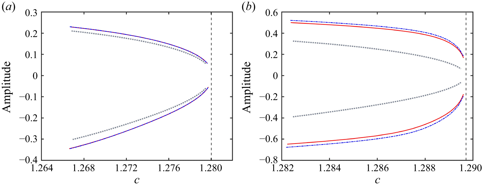
with $\varPsi =cZ$ . We solve (4.36) using the Newton–Raphson method, considering a solution converged when the $L^\infty $ -norm of the residual error is less than $10^{-10}$ . Once we find one solution, we compute others along the same bifurcation branch using straightforward numerical continuation. The computation of solitary waves in the model (4.6) and (4.10) follows a similar approach. Unlike the work of Gao et al. (Reference Gao, Wang and Vanden-Broeck2016), this study introduces the inertia effect into the hydroelastic wave system. Nevertheless, we are still able to identify two fundamental branches of solitary waves: elevation waves (which have a positive free-surface displacement at the centre) and depression waves (which have a negative free-surface displacement at the centre), as shown in figure 3. These solutions exhibit oscillatory decaying tails and are referred to as wavepacket solitary waves. As illustrated in figure 3, the cubic DNO-truncation model shows consistently better agreement with the Euler solutions compared with the quadratic DNO-truncation model in both shallow and deep-water scenarios. However, due to the weakly nonlinear nature of the cubic model, discrepancies between this model and the Euler results become more pronounced for large-amplitude solitary waves in deep water, highlighting the former’s limitations in strongly nonlinear regimes. It should be noted that the parameters used in these computations are derived from table 1, which includes the experiment in Lake Saroma for the shallow-water case ( $\alpha =0.0691$ ) and the experiment in McMurdo Sound for the deep-water scenario ( $\alpha =0.0717$ ).

Figure 3.

Speed-amplitude bifurcation diagrams for solitary waves in the 2-D problem: comparison of the quadratic model (grey dotted lines), the cubic model (blue dash-dotted lines) and the full Euler equations (red solid lines). The vertical dashed lines indicate the phase speed minima, labelled as $c^{\ast }$ . In panel (a), the water depth is $h=6.8\,\mathrm{m}$ with a corresponding $c^{\ast }=1.2800$ , while panel (b) represents the case of infinite water depth ( $h\to \infty$ ), where $c^{\ast }=1.2897$ .

Figure 4.

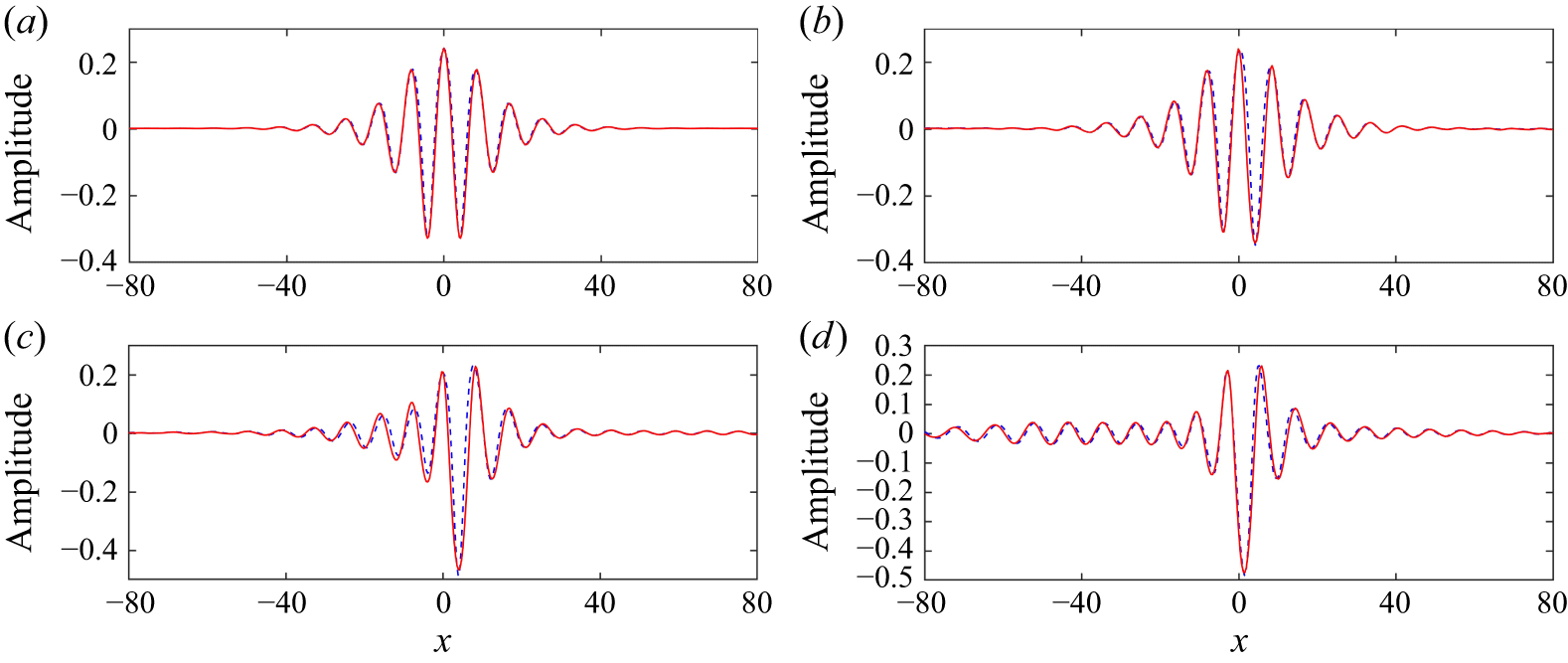
Time evolution of an elevation solitary wave under a small perturbation in shallow water ( $h=6.8\,\mathrm{m}$ ). The red solid lines represent the results from the full Euler equations, while the blue dashed lines reflect the results from the cubic model. Snapshots are captured at: (a) $t=0$ ; (b) $t=160$ ; (c) $t=290$ , and (d) $t=600$ . Perturbation parameter is set as $\delta =-0.05$ and the initial wave speed is $c=1.2614$ .

Studies conducted by Wang & Milewski (Reference Wang and Milewski2012) and Gao et al. (Reference Gao, Wang and Vanden-Broeck2016) demonstrate that elevation solitary waves become unstable when subjected to small perturbations. To further validate the effectiveness of the cubic model, we compare its time-dependent results for the long-term dynamics of an unstable elevation wave with those obtained from the full Euler equations. We introduce a perturbation to the exact solitary wave solution by applying a small multiple of itself, using the initial condition $\eta (x,0)=(1+\delta )\widetilde {\eta }$ , where $\widetilde {\eta }$ represents the computed travelling wave and $\delta$ is a small constant. For the time-dependent simulations, the configuration of the computational domain remains unchanged from the previous specification, with a time step of $\Delta t=0.001$ employed. The results, shown in figures 4 and 5, reveal a remarkable consistency between the Euler solutions and the simulations produced by the cubic model for both shallow and deep water cases, thereby confirming the model’s effectiveness. Additionally, we independently simulate overtaking collisions between two depression solitary waves using both the full Euler equations and the cubic model, with the results illustrated in figures 6 and 7. Our simulations of the cubic model in shallow water align more closely with the Euler solutions than those in deep water. This discrepancy is primarily due to the model’s weakly nonlinear nature; specifically, the amplitude of solitary waves is generally larger in deep water than in shallow water.

Figure 5.

Time evolution of an elevation solitary wave under a small perturbation in deep water ( $h\to \infty$ ). The red solid lines represent the results from the full Euler equations, while the blue dashed lines reflect the results from the cubic model. Snapshots are captured at: (a) $t=0$ ; (b) $t=130$ ; (c) $t=170$ and (d) $t=350$ . Perturbation parameter is set as $\delta = -0.05$ and the initial wave speed is $c = 1.2804$ .

Figure 6.

An overtaking collision between two depression solitary waves with different speeds ( $c=1.2727$ and $c=1.2469$ ) in shallow water ( $h=6.8\,\mathrm{m}$ ). The results are plotted in a frame of reference moving at the speed of the slower one. The red solid lines indicate the results from the full Euler equations, and the blue dashed lines represent the results from the cubic model. Snapshots are captured at the following times: (a) $t=0$ ; (b) $t=3200$ and (c) $t=4500$ .

Figure 7.

An overtaking collision between two depression solitary waves with different speeds ( $c=1.2870$ and $c=1.2680$ ) in deep water. The results are plotted in a frame of reference moving at the speed of the slower one. The red solid lines indicate the results from the full Euler equations, while the blue dashed lines represent the results from the cubic model. Snapshots are taken at the following times: (a) $t=0$ ; (b) $t=1100$ and (c) $t=3500$ .

The previous discussion regarding the 2-D problem illustrates the effectiveness of the cubic DNO-truncation model, particularly in terms of the bifurcation mechanism and dynamic behaviour of wavepacket solitary waves, which closely resemble the solutions of the full Euler equations. In contrast, the quadratic DNO-truncation model fails to accurately capture the associated NLS equation at the minimum phase speed, leading to significant deviations from the Euler equations. For the 3-D hydroelastic wave problem, wavepacket solitary waves are characterised by oscillatory decaying tails in the direction of wave propagation and monotonicity in the transverse direction. These waves have been demonstrated, both asymptotically and numerically, in previous studies (Milewski & Wang Reference Milewski and Wang2013; Trichtchenko et al. Reference Trichtchenko, Părău, Vanden-Broeck and Milewski2018). These solutions are commonly referred to as lumps. Figure 8 displays the speed-amplitude bifurcation curves obtained from the quadratic and cubic models for hydroelastic lumps. Notable differences appear between the two models in both shallow-water and deep-water scenarios. For a given wave speed, the quadratic model predicts a slightly lower wave amplitude than the cubic model in shallow water and this discrepancy becomes more pronounced in deep water. It is observed that the BRDS equation for both cases, $h=6.8$ and $h\to \infty$ , is focusing, although the values of $\varXi$ differ between the two scenarios. However, in the deep, the significant difference in $\varXi$ between the quadratic and cubic models, as illustrated in figure 2, leads to significant gaps in the speed-amplitude bifurcation diagrams. In addition to the reduced models, hydroelastic lumps can also be simulated using the boundary integral equation method (Părău & Vanden-Broeck Reference Părău and Vanden-Broeck2002; Trichtchenko et al. Reference Trichtchenko, Părău, Vanden-Broeck and Milewski2018; Părău & Vanden-Broeck Reference Părău and Vanden-Broeck2019; Ţugulan et al. Reference Ţugulan, Trichtchenko and Părău2022). However, this approach is computationally expensive when aiming for highly accurate results (see, for example, Wang & Milewski Reference Wang and Milewski2012). Lastly, accurately simulating unsteady 3-D hydroelastic waves using the full Euler equations is substantially more complex. Therefore, we adopt the cubic DNO-truncation model in the subsequent sections to reduce computational costs while maintaining physical accuracy.

Figure 8.

Speed-amplitude bifurcation diagrams for hydroelastic lumps in the 3-D problem: comparison between the quadratic (grey dotted lines) and cubic (blue dash-dotted lines) models. The leading-order prediction (4.28) is shown with a red line for the shallow-water case. The vertical dashed lines represent the phase speed minima, labelled as $c^{\ast }$ . In panel (a), the water depth is $h=6.8\mathrm{m}$ with a corresponding $c^{\ast }=1.2800$ , while panel (b) represents the case of infinite water depth ( $h\to \infty$ ) with $c^{\ast }=1.2897$ .

6.1. Responses to uniformly accelerating loads

Previous studies have primarily examined the response of a floating ice sheet to a load that is suddenly applied and then moves steadily, without any acceleration. Notable exceptions to this focus are the research contributions of Miles & Sneyd (Reference Miles and Sneyd2003), Dinvay et al. (Reference Dinvay, Kalisch and Părău2019) and Hosking & Milinazzo (Reference Hosking and Milinazzo2022). Miles & Sneyd (Reference Miles and Sneyd2003) and Hosking & Milinazzo (Reference Hosking and Milinazzo2022) employed a 2-D linear theory to explore how a floating ice sheet reacts to a line load moving at variable speeds, whereas Dinvay et al. (Reference Dinvay, Kalisch and Părău2019) analysed the deceleration process of a moving load using a fully dispersive model. Both Dinvay et al. (Reference Dinvay, Kalisch and Părău2019) and Hosking & Milinazzo (Reference Hosking and Milinazzo2022) found that deceleration from supercritical velocities can lead to a significantly amplified deflection. This occurs due to constructive interference as trailing, gravity-dominated waves catch up to the slowing load. To examine how acceleration and deceleration affect ice deflection in three dimensions and to investigate constructive interference, the following two subsections use the validated cubic model to analyse the transient response to a load with variable velocity. Unlike the travelling-wave solutions discussed earlier, the scenarios of acceleration and deceleration are time-dependent, resulting in a relatively short computational duration. However, this brief time scale allows the waves generated during speed transitions – typically expected to radiate away in an unbounded domain – to traverse the periodic boundaries and re-enter the computational domain, potentially contaminating the numerical results. To address this issue, a sponge layer is introduced following the work of Guyenne & Părău (Reference Guyenne and Părău2017). This involves adding a damping pressure term, represented as

(6.1) \begin{equation} -\!\Lambda (x,y)G(\eta )\xi, \end{equation}

to the right-hand side of (4.2), where $\varLambda$ is a tuneable, spatially dependent coefficient that is non-zero only in a small region near the boundary. A $\text{tanh}$ profile is used to illustrate the localised spatial behaviour of $\Lambda (x,y)$ , expressed as

(6.2) \begin{equation} \begin{aligned} \varLambda (x,y)=&\,\mu\! \left \{\text{tanh}\left [2\pi \left (x-x_e+\frac {l_{\!p}}{2}\right )\right ]-\text{tanh}\left [2\pi \left (x-x_s+\frac {l_{\!p}}{2}\right )\right ]\right .\\ &\,+\left .\text{tanh}\left [2\pi \left (y-y_e+\frac {l_{\!p}}{2}\right )\right ]-\text{tanh}\left [2\pi \left (y-y_s+\frac {l_{\!p}}{2}\right )\right ]+4\right \}\!, \end{aligned} \end{equation}

where $\mu$ is a constant, $l_{\!p}$ denotes the approximate width of the sponge layer, and $x_e,\,y_e$ and $x_s,\,y_s$ represent the right and left boundaries of the domain in horizontal directions, respectively. Numerical tests indicate that setting $\mu =80$ and $l_{\!p}=10$ effectively mitigates the impact of outgoing disturbances. Since the characteristics of waveforms in deep water do not differ qualitatively from those in shallow water, the variable-speed load analysis is conducted in shallow water, using all physical parameters derived from the experimental observations of Takizawa (Reference Takizawa1985).

Building on the work of Miles & Sneyd (Reference Miles and Sneyd2003) and Hosking & Milinazzo (Reference Hosking and Milinazzo2022), we begin by analysing the transient responses of a floating ice sheet to a load experiencing a constant acceleration $a_c$ that starts at $t=0$ . The corresponding position of the load is given by

(6.3) \begin{equation} X(t)=\left \{ \begin{aligned} &\frac 12a_ct^2, &&0\leqslant t\lt T_c,\\[5pt] &\frac 12a_cT_c^2+V(t-T_c), &&t\geqslant T_c, \end{aligned}\right . \end{equation}

where $V$ denotes the final velocity of the load and $T_c$ represents the acceleration time. For reference, a steadily moving load (discussed in previous sections) corresponds to an impulsive start, characterised by the position function $X(t)=Vt$ for $t\geqslant 0$ , where $V$ is constant. Due to the absence of ready-made experiments for comparison, we present numerical cross-sectional profiles at $y=0\,\mathrm{m}$ to highlight the effects of acceleration, where ice deflection is maximised. The load is positioned at the origin in the plots. Numerical simulations reveal that the effects of acceleration become negligible when the final load velocity is sufficiently low compared with the critical speed. Therefore, we focus on two specific cases with final velocities of $V=6.2\,\mathrm{m}\,\rm s^{-1}$ and $V=8.9\,\mathrm{m}\,\rm s^{-1}$ , where the effects of acceleration are more pronounced.

Figure 16.

Maximum ice deflection (in mm) as a function of time $t$ (in s), which is calculated by the cubic model and measured at $y=0\,\mathrm{m}$ . The grey curve represents a load that starts impulsively with a constant velocity ( $a_c=0\,\mathrm{m}\,\rm s^{-2}$ ) and reaches a final velocity of $6.2\,\mathrm{m}\,\rm s^{-1}$ . The blue curve corresponds to an acceleration of $a_c=2\,\mathrm{m}\,\rm s^{-2}$ , while the red curve indicates $a_c=1.5\,\mathrm{m}\,\rm s^{-2}$ and the green curve represents $a_c=1\,\mathrm{m}\,\rm s^{-2}$ . The left side of the dotted line illustrates the uniformly accelerated process, while the right side depicts the uniform motion process.

Figure 17.

Maximum ice deflection (in mm) as a function of time $t$ (in s), which is calculated by the cubic model and measured at $y=0\,\mathrm{m}$ . The grey curve represents a load that starts impulsively with a constant velocity ( $a_c=0\,\mathrm{m}\,\rm s^{-2}$ ) and reaches a final velocity of $8.9\,\mathrm{m}\,\rm s^{-1}$ . The blue curve corresponds to an acceleration of $a_c=2\,\mathrm{m}\,\rm s^{-2}$ , while the red curve indicates $a_c=1.5\,\mathrm{m}\,\rm s^{-2}$ and the green curve represents $a_c=1\,\mathrm{m}\,\rm s^{-2}$ . The left side of the dotted line illustrates the uniformly accelerated process, while the right side depicts the uniform motion process.

When the target velocity reaches $6.2\,\mathrm{m}\,\rm s^{-1}$ , the numerical results in figure 16 indicate that the acceleration process reduces the growth rate of ice deflection; however, this effect is relatively weak. Conversely, when the final load velocity significantly exceeds $c_{\textit{min}}$ , as illustrated in figure 17, the acceleration process increases the maximum ice deflection, with the amplification becoming more pronounced as the acceleration duration increases. This phenomenon can be explained by considering that the load spends more time in the two-wave stage, as shown in figure 11, where the ice deflection is inherently greater. Additionally, a smaller acceleration allows for a longer duration to generate waves while the load is in this two-wave stage. As the load velocity increases, it gradually overtakes the waves generated during its earlier acceleration phase. This leads to constructive interference, which will be discussed in detail in the next subsection, resulting in an increased ice deflection. These findings have practical implications for vehicle operation on ice sheets: when travelling at high speeds (exceeding the critical velocity $c_{\textit{min}}$ and approaching $c_0$ ), a shorter acceleration time – achieved by a higher acceleration – would enhance safety.

While the previous discussion focuses on loads that start from rest, we will now examine scenarios where acceleration begins from steady, uniform motion. This approach allows us to isolate the effects of speed changes, independent of any startup transients. The central position of the load can be expressed as

(6.4) \begin{equation} X(t)=\left \{ \begin{aligned} &\frac 12V_0t, &&0\leqslant t\lt T_u,\\[5pt] &\frac 12V_0t+\frac {1}{2}a_c(t-T_u)^2, &&T_u\leqslant t\lt T_u+T_c,\\[5pt] &\frac 12V_0t+\frac {1}{2}a_cT_c^2+(V-V_0)(t-T_u-T_c), &&t\geqslant T_u+T_c, \end{aligned}\right . \end{equation}

where $V_0$ is the initial constant velocity of the load and $T_u$ represents the time during which the load moves at this constant velocity. Here, $T_u$ is chosen to be sufficiently long to ensure that the ice deflection reaches a steady state before the acceleration begins. In this scenario, the initial velocity of the load is $V_0=2.2\,\mathrm{m}\,\rm s^{-1}$ , with final velocities of $V=6.2\,\mathrm{m}\,\rm s^{-1}$ and $V=8.9\,\mathrm{m}\,\rm s^{-1}$ . Although not presented graphically, the numerical results indicate little difference compared with the impulsively started case, suggesting a degree of independence from the selection of initial velocity.

6.2. Response to a uniformly decelerating load

In this section, we examine the ice deflection caused by a load that is undergoing a constant deceleration $a_d$ from the initial velocity $V$ . The corresponding load position is given by

(6.5) \begin{equation} X(t)=\left \{ \begin{aligned} &\textit{Vt}, &&0\leqslant t\lt T_u,\\ &\textit{Vt}+\frac 12a_d(t-T_u)^2, &&T_u\leqslant t\lt T_u+T_d,\\ &\textit{VT}_d+\frac 12a_dT_d^2, &&t\geqslant T_u+T_d, \end{aligned}\right . \end{equation}

where $T_u$ represents the time during which the load moves at a constant velocity and $T_d$ denotes the time of deceleration. After the load’s speed decreases to zero, it remains stationary. To avoid interference from startup transients, $T_u$ is set to a duration long enough to ensure that the ice deflection reaches a steady state before deceleration commences. Based on the previous subsection, the deceleration analysis focuses on two initial velocities: $V=6.2\,\mathrm{m}\,\rm s^{-1}$ and $8.9\,\mathrm{m}\,\rm s^{-1}$ . The motion of deceleration generates more complex wave patterns compared with acceleration. As a result, figures 18 and 19 present cross-sectional snapshots of the ice deflection. These figures clearly illustrate the temporal evolution of ice deflection during and after deceleration, highlighting the emergence and effects of constructive interference.

Figure 18.

A comparison of numerical simulations that start with an initial velocity of $V=6.2\,\mathrm{m}\,\rm s^{-1}$ and vary the deceleration in a shallow water scenario. The vertical coordinate ( $\eta$ , in mm) indicates ice deflection, while the horizontal coordinate ( $x$ , in m) represents displacement. Snapshots are taken at the following times: (a) 0.758 s; (b) 1.56 s; (c) 2.32 s; (d) 3.10 s; (e) 3.88 s; ( f) 4.64 s; (g) 5.45 s; (h) 6.20 s; (i) 7.82 s and ( j) 9.47 s. The moment when the load starts to accelerate or decelerate is defined as zero time. Blue solid curves depict the load moving with a uniform deceleration of $a_d=-2\,\mathrm{m}\,\rm s^{-2}$ , while grey dotted curves represent a deceleration of $a_d=-1\,\mathrm{m}\,\rm s^{-2}$ .

Figure 19.

A comparison of numerical simulations that start with an initial velocity of $V=8.9\,\mathrm{m}\,\rm s^{-1}$ and vary the deceleration in a shallow-water scenario. The vertical coordinate ( $\eta$ , in mm) indicates ice deflection, while the horizontal coordinate ( $x$ , in m) represents displacement. Snapshots are taken at the following times: (a) 1.09 s; (b) 2.23 s; (c) 3.32 s; (d) 4.45 s; (e) 5.54 s; ( f) 6.68 s; (g) 7.77 s; (h) 8.90 s; (i) 10.7 s and (j) 11.8 s. The moment when the load starts to accelerate or decelerate is defined as zero time. Blue curves depict the load moving with a uniform deceleration of $a_d=-2\,\mathrm{m}\,\rm s^{-2}$ , while grey curves represent a deceleration of $a_d=-1\,\mathrm{m}\,\rm s^{-2}$ .

Constructive interference can be understood as the superposition of the deflection caused by the quasi-static load and the waves generated by its motion. Changes in the speed of the load may result in a relative displacement between the load and the waves it produces. When the depression pulse created by the load coincides with the trough of the generated waves, the amplitude of the depression increases, as illustrated in figures 18(g) and 18(j). In contrast, when the load aligns with the wave crest, the amplitude of the depression decreases, which can be seen in figures 18(e), 18(i) and 19(e). Once the load stops and remains stationary, the generated waves gradually detach from the static depression, resulting in the fading of constructive interference (see figures 19 g–19 j).

Figure 20.

A wave profile comparison under various deceleration rates at different moments. The blue curves represent the load that is decelerating uniformly at a rate of $a_d=-2\,\mathrm{m}\,\rm s^{-2}$ , with snapshots taken at the following times: (a) 3.10 s; (b) 3.88 s; (c) 4.64 s and (d) 7.82 s. The grey curves indicate the load that is decelerating uniformly at a rate of $a_d=-1\,\mathrm{m}\,\rm s^{-2}$ , with snapshots taken at the following times: (a) 4.64 s; (b) 5.45 s; (c) 6.20 s and (d) 9.47 s.

When the initial speed of the load is close to $c_{\textit{min}}$ , the gravity waves generated behind the load can catch up with it during deceleration, leading to constructive interference. However, if the load’s speed exceeds the long-wave limiting velocity $c_0$ , a shadow zone forms behind the load. In this scenario, constructive interference can occur from the generated gravity waves when the load decelerates to the two-wave stage. The stronger presence of waves behind the load during the initial phase, as illustrated in figure 18, contrasts with the situation shown in figure 19, leading to greater constructive interference. Similar to the acceleration results discussed earlier, both figures 18 and 19 demonstrate that changes in deceleration do not alter the evolution of ice deflection; instead, they impact the rate of change. For example, the deflection patterns for a deceleration of $a_d=-2\,\mathrm{m}\,\rm s^{-2}$ in figures 18(d)–18( f) and 18(i) closely resemble those for a lower deceleration of $a_d = -1\,\mathrm{m}\,\rm s^{-2}$ in figures 18( f)–18(h) and 18(j). These similar patterns are directly compared in figure 20.

Figure 21.

Maximum ice deflection (in $\mathrm{mm}$ ) as a function of time $t$ (in s), starting from $V=6.2\,\mathrm{m}\,\rm s^{-1}$ . It is calculated by the cubic model and measured at $y=0\,\mathrm{m}$ . The blue curve corresponds to a deceleration of $a_d=-2\,\mathrm{m}\,\rm s^{-2}$ , while the red curve indicates $a_d=-1.5\,\mathrm{m}\,\rm s^{-2}$ and the green curve represents $a_d=-1\,\mathrm{m}\,\rm s^{-2}$ . The load’s velocity decreases to zero at the vertical dotted lines.

Figure 22.

Maximum ice deflection (in $\mathrm{mm}$ ) as a function of time $t$ (in s), starting from $V=8.9\,\mathrm{m}\,\rm s^{-1}$ . It is calculated by the cubic model and measured at $y=0\,\mathrm{m}$ . The blue curve corresponds to a deceleration of $a_d=-2\,\mathrm{m}\,\rm s^{-2}$ , the red curve indicates $a_d=-1.5\,\mathrm{m}\,\rm s^{-2}$ and the green curve represents $a_d=-1\,\mathrm{m}\,\rm s^{-2}$ . The load’s velocity decreases to zero at the vertical dotted lines.

Following the approach in the previous section, we also plot the temporal variation of the maximum ice deflection in figures 21 and 22. When the load’s initial velocity is close to $c_{\textit{min}}$ ( $V=6.2\,\mathrm{m}\,\rm s^{-1}$ ), the deceleration process not only reduces the maximum ice deflection, but also introduces oscillatory behaviour, without significantly increasing its peak value. Over time, the maximum ice deflection gradually approaches a steady-state value amid these oscillations, although computational limitations prevent us from simulating the process to full convergence. In contrast, at a higher initial velocity of $V=8.9\,\mathrm{m}\,\rm s^{-1}$ , the deceleration results in an increased maximum deflection, with peak values rising as the deceleration time is extended. Therefore, for safety reasons, rapid braking is preferable to gradual deceleration. Additionally, the deflection pattern in figure 19( f) resembles figure 11 from Dinvay et al. (Reference Dinvay, Kalisch and Părău2019) and figure 12(a) from Hosking & Milinazzo (Reference Hosking and Milinazzo2022). As observed with the initial speed of $V=6.2\,\mathrm{m}\,\rm s^{-1}$ , the maximum ice deflection ultimately converges to a steady value. The fluctuations observed are due to constructive interference. Since this interference is relatively weak, the maximum ice deflection converges quicker.

It is worth noting that the temporal evolution curves in figure 21 are less smooth than those in figures 16, 17 and 22. In figure 19, the maximum ice deflection typically occurs directly beneath the load. However, a special situation is observed in figure 18(c), where constructive interference causes the maximum deflection to shift away from the load position to nearby troughs. As the generated waves subsequently detach from the load, the maximum deflection relocates to the trough directly beneath the load, resulting in jagged curves seen in figure 21.

6.3. Validation

To validate the accuracy of the cubic model for simulating the response of a variable-velocity load, numerical results are compared with the linear analytical solution provided in (3.9). Evaluating this solution necessitates the use of numerical methods due to its complex temporal integral. The time integral can be computed efficiently using the recurrence relations (3.11) and (3.12). The calculation involves evaluating operators using the fast Fourier transform and its inverse. To ensure the accuracy of the results, the time step size is set at $\Delta T=0.00001$ , while all other physical parameters remain consistent with those used in the preceding sections.

Figure 23.

A comparison between the analytical solution derived from linear theory and numerical simulations of the cubic model at various times: (a) 1.56 s; (b) 3.10 s; (c) 4.64 s and (d) 6.20 s. The left side corresponds to the acceleration case with $a_c=1\,\mathrm{m}\,\rm s^{-2}$ , while the right side represents the deceleration case with $a_d=-1\,\mathrm{m}\,\rm s^{-2}$ . In both cases, the final and initial velocities are $V=6.2\,\mathrm{m}\,\rm s^{-1}$ . The vertical coordinate ( $\eta$ , in mm) indicates ice deflection, whereas the horizontal coordinate ( $x$ , in m) represents displacement. The red curves illustrate the analytical solutions and the blue curves depict the numerical simulations of the cubic model, with the load positioned at the origin.

Taking examples of uniformly accelerated motion ( $a_c=1\,\mathrm{m}\,\rm s^{-2}$ ) and uniformly decelerated motion ( $a_d=-1\,\mathrm{m}\,\rm s^{-2}$ ), comparative results are shown in figure 23. There is excellent agreement between the linear analytical solutions and the results from the cubic model, which confirms the model’s effectiveness in simulating variable-velocity load problems. This agreement reflects the predominantly linear behaviour of the system during variable-speed motion of the load, consistent with the findings of Miles & Sneyd (Reference Miles and Sneyd2003), Johnsen et al. (Reference Johnsen, Kalisch and Părău2022) and Hosking & Milinazzo (Reference Hosking and Milinazzo2022). Finally, we should emphasise that using a variable speed method, whether through acceleration or deceleration, is an effective approach to swiftly cross the critical speed and prevent substantial deformation of ice covers in practice.