
1. Introduction
The flow around a finite wall-mounted cylinder (FWMC) continues to be an active area of research due to its diverse environmental and engineering applications, and fundamental importance in advancing physical insight into complex turbulent shear flows. Examples of practical applications include atmospheric boundary layer over low- and high-rise buildings, wind turbines and chimney stacks, ocean currents around offshore structures and tidal turbines and river flow around aquatic vegetation. In these applications, the flow around the FWMC is characterized by unsteady three-dimensional (3-D) flow structures that are concurrently influenced by the free end of the cylinder and the bottom wall. These competing end effects can dramatically alter the quasi-periodic Kármán vortex shedding from the sides of the FWMC and complicate the flow physics compared to two-dimensional (2-D) or infinite cylinders. In general, vortex shedding behind FWMCs is an important phenomenon in many engineering applications as it can lead to vortex-induced vibrations, resonance, noise generation and fatigue failure. Therefore, comprehensive investigations on the unsteady 3-D wake structure of FWMCs are essential for improving our understanding of the flow physics and developing optimal flow-control strategies for mitigating structural vibrations.
Several experimental and numerical studies have been conducted in the past to investigate the wake structure of FWMCs using geometries such as circular cylinders (Sumner, Heseltine & Dansereau Reference Sumner, Heseltine and Dansereau2004; Pattenden, Turnock & Zhang Reference Pattenden, Turnock and Zhang2005; Krajnović Reference Krajnović2011; Tang et al. Reference Tang, Jiang, Zheng and Wu2016; Heidari et al. Reference Heidari, Balachandar, Roussinova and Barron2017; Hamed & Peterlein Reference Hamed and Peterlein2020) and cylinders with sharp edges (Balachandar & Tachie Reference Balachandar and Tachie2001; Wang et al. Reference Wang, Zhou, Chan and Lam2006; Wang & Zhou Reference Wang and Zhou2009; Bourgeois, Sattari & Martinuzzi Reference Bourgeois, Sattari and Martinuzzi2011; Nasif, Balachandar & Barron Reference Nasif, Balachandar and Barron2015; Yauwenas et al. Reference Yauwenas, Porteous, Moreau and Doolan2019). While most of the previous studies examined the FWMC in a uniform flow (Farivar Reference Farivar1981; Okamoto & Yagita Reference Okamoto and Yagita1973; Fox, Apelt & West Reference Fox, Apelt and West1993) or thin turbulent boundary layer (TBL) ( $\delta \ll h$, where δ is the boundary layer thickness and h is the cylinder height) (Pattenden et al. Reference Pattenden, Turnock and Zhang2005; Wang & Zhou Reference Wang and Zhou2009; Krajnović Reference Krajnović2011; Yauwenas et al. Reference Yauwenas, Porteous, Moreau and Doolan2019), a FWMC that is fully immersed in a thick TBL (δ > h as illustrated in figure 1) has received less attention, though encountered in many of the aforementioned practical applications. For δ > h, the FWMC encounters stronger mean shear and higher turbulence intensity in the approach flow, which can further complicate the unsteady flow separation and wake dynamics of the cylinder compared to its counterpart in a uniform flow or thin TBL. The aim of this work is, therefore, to provide a detailed investigation on the unsteady wake characteristics of circular FWMCs fully immersed in a thick TBL at different submergence ratios (δ/h).
A circular FWMC of diameter, d and height, h fully immersed in a TBL of free-stream velocity,  ${U_\infty }$ and boundary layer thickness, δ. The left-handed Cartesian coordinate system adopted has the origin of the streamwise (x), wall-normal (y) and spanwise (z) directions at the centre of the cylinder on the bottom wall.
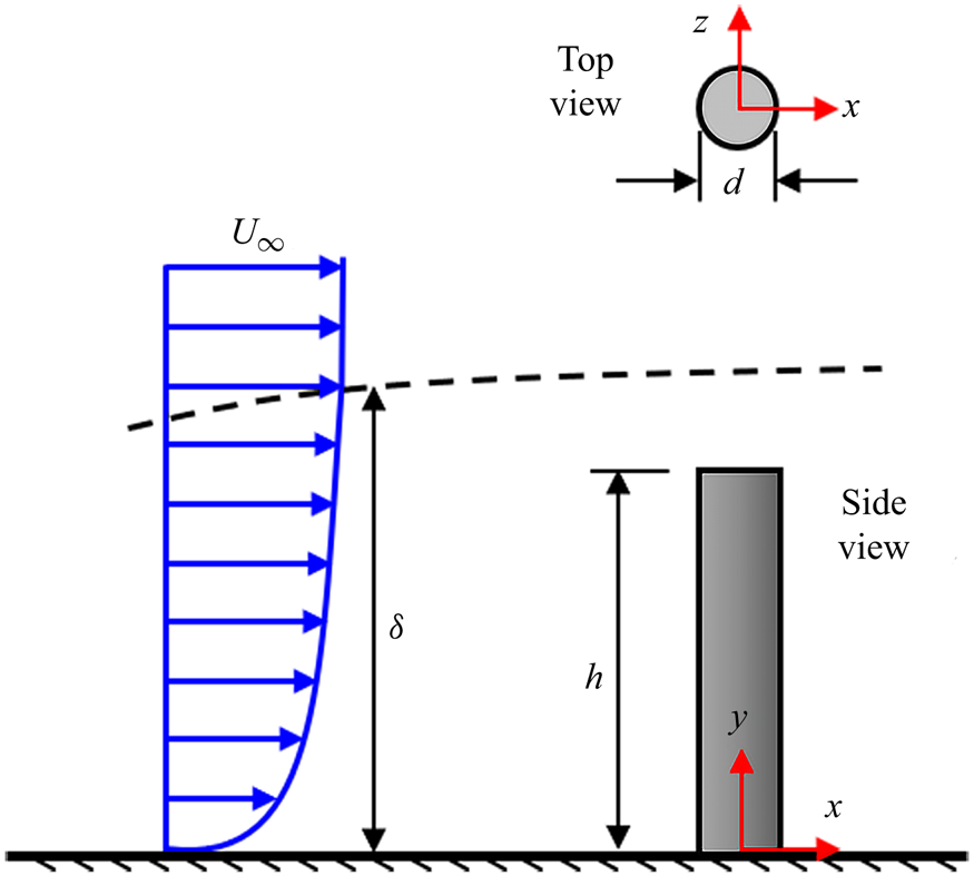
The circular FWMC is a simple geometry yet exhibits complex physical phenomena such as flow separation, shear layer interactions, vortex formation, shedding and merging and interactions between different vortical structures. These flow features are dependent on three main parameters: Reynolds number,  $Re = {U_\infty }d/\nu $ (where
 ${U_\infty }$ is the free-stream velocity, d is the diameter of the cylinder and
 $\nu $ is the kinematic viscosity), aspect ratio, h/d, and δ/h (Zdravkovich Reference Zdravkovich1997; Sumner et al. Reference Sumner, Heseltine and Dansereau2004; Porteous, Moreau & Doolan Reference Porteous, Moreau and Doolan2014).
Unlike the FWMCs with sharp edges, the Reynolds number has a strong influence on the location and type of separation (laminar or turbulent) along the sides of the circular cylinder. The lack of a fixed separation location and its dependence on Reynolds number can pose significant challenges to numerical simulations. Indeed, the circular cylinder is routinely used as an acute test case for assessing the predictive capability of numerical turbulence models (Travin et al. Reference Travin, Shur, Strelets and Spalart2000; Benim, Pasqualotto & Suh Reference Benim, Pasqualotto and Suh2008; Ünal, Atlar & Gören Reference Ünal, Atlar and Gören2010). According to Zdravkovich (Reference Zdravkovich1997), the Reynolds number can be used to categorize the flow past a circular cylinder in a uniform flow into four main regimes: subcritical  $(4 \times {10^2} \lt Re \lt {10^5})$, critical
 $({10^5} \lt Re \lt 3 \times {10^5})$, supercritical
 $(3 \times {10^5} \lt Re \lt 2 \times {10^6})$ and transcritical
 $(Re \gt 2 \times {10^6})$ regimes. In the subcritical regime, laminar separation occurs on the sides of the cylinder at an angle of 70°–80° from the front stagnation line and the transition to turbulence proceeds in the separated shear layers. Norberg (Reference Norberg1994) found that the subcritical regime also exhibits differences in vortex shedding behaviour for flows within the lower and upper bounds of the regime demarcated by
 $Re = 5 \times {10^3}$. In the critical regime, the laminar separation transitions to a turbulent state and reattaches on the cylinder, leading to the formation of laminar separation bubble. This is followed by a turbulent separation which leads to a significant reduction in drag. The supercritical and transcritical regimes, on the other hand, are characterized by turbulent separation and the separation line moves towards the front part of the cylinder as Reynolds number increases. It is worth noting that most of the previous studies were conducted at Reynolds numbers in the subcritical regime. Comprehensive reviews of these studies and the parameters investigated are well documented in Palau-Salvador et al. (Reference Palau-Salvador, Stoesser, Fröhlich, Kappler and Rodi2010), Sumner (Reference Sumner2013) and Porteous et al. (Reference Porteous, Moreau and Doolan2014).
The effects of aspect ratio on the wake structure of circular FWMCs have also been studied (West & Apelt Reference West and Apelt1982; Szepessy & Bearman Reference Szepessy and Bearman1992; Norberg Reference Norberg1994; Park & Lee Reference Park and Lee2000, Reference Park and Lee2002; Sumner et al. Reference Sumner, Heseltine and Dansereau2004), yet not completely understood because of the interconnection between aspect ratio and submergence ratio. Previous studies have shown that at a critical aspect ratio, the Kármán vortex shedding, which is usually defined by the Strouhal number,  $St\; = {f_s}d/{U_\infty }$ (where fs is the shedding frequency) is suppressed signifying a change in the wake structure of the cylinder (Kawamura et al. Reference Kawamura, Hiwada, Hibino, Mabuchi and Kumada1984; Sumner et al. Reference Sumner, Heseltine and Dansereau2004; Moreau & Doolan Reference Moreau and Doolan2013). However, the critical aspect ratio reported in previous investigations varies from h/d = 1 to 7. The major reason for this disparity is the influence of the submergence ratio (Porteous et al. Reference Porteous, Moreau and Doolan2014), which has not been systematically examined in the literature.
Figure 2 shows the salient features of the wake structure of circular FWMCs with aspect ratios higher (figure 2a) and lower (figure 2b) than an arbitrary critical value. The flow structure on the free end of the cylinder is also illustrated in figure 2(c). The figure is based on the time-averaged models proposed by Pattenden et al. (Reference Pattenden, Turnock and Zhang2005), Frederich et al. (Reference Frederich, Wassen, Thiele, Jensch, Brede, Hüttmann, Leder, Tropea, Jakirlic, Heinemann, Henke and Hönlinger2007) and Krajnović (Reference Krajnović2011) and the review on the free-end flow structure of a circular FWMC by Sumner (Reference Sumner2013). For each cylinder, the approach flow encounters a higher stagnation pressure in front of the cylinder which causes part of the flow to deflect upwards and over the free end of the cylinder. The other part deflects downwards leading to the formation of the well-known horseshoe vortex system with legs wrapped around the cylinder, extending on either side while interacting partly with the wake. The horseshoe vortex system may consist of a primary or dominant horseshoe vortex and other weaker secondary and tertiary vortices. As shown in figure 2(c), the flow deflected over the free end separates at the leading edge of the cylinder and attaches on the top surface of the cylinder. The mean attachment length, Xr defined as the streamwise distance from the leading edge to the attachment point on the centreline of the cylinder is strongly influenced by the aspect ratio and the submergence ratio (Sumner Reference Sumner2013). For h/d < 1, the mean attachment length increases with increasing aspect ratio but gradually decreases for h/d > 2 (Sumner et al. Reference Sumner, Rostamy, Bergstrom and Bugg2015). The attachment line also moves further upstream towards the leading edge as δ/h increases (Kawamura et al. Reference Kawamura, Hiwada, Hibino, Mabuchi and Kumada1984; Tsutsui Reference Tsutsui2012), however, these observations have not been examined in detail for FWMCs fully immersed in a TBL. After attachment, part of the flow deflects upstream (reverse flow) to form the primary recirculation region on the top surface of the cylinder. The reverse flow approaching the leading edge is opposed by the separated shear layer which results in the formation of a secondary recirculation region near the leading edge and a redirection of the reverse flow towards the two sides of the cylinder to form localized recirculation regions on either side of the centreline. The foci of the two localized recirculation regions are footprints of the free-end arch vortex that bends laterally over the surface through the focus of the primary recirculation region. The secondary recirculation region, on the other hand, forms part of the leading-edge vortex that stretches along the frontal edge of the surface. Downstream of the attachment line, the forward free-end flow interacts with the wake behind the cylinder leading to the formation of the upper near-wake cross-stream vortex (Bt).
Schematic of time-averaged flow configuration of a circular FWMC with (a) aspect ratio, h/d > critical value and (b) h/d < critical value. (c) Schematic of the free-end salient flow features of a circular FWMC. The sketches are based on models proposed by Pattenden et al. (Reference Pattenden, Turnock and Zhang2005), Frederich et al. (Reference Frederich, Wassen, Thiele, Jensch, Brede, Hüttmann, Leder, Tropea, Jakirlic, Heinemann, Henke and Hönlinger2007) and Krajnović (Reference Krajnović2011). The labels are Bt – upper near-wake cross-stream vortex, Nv – near-wake base vortex, H 2 – secondary horseshoe vortex and Xr – mean attachment length on the top surface of the cylinder.

On the sides of the cylinder, the flow separates but the separation line is usually bent towards the rear of the free end and bottom of the cylinder. Near the free end, the delay in separation is caused by the interaction of flow along the upper part of the cylinder and the flow over the edges of the free end which leads to the formation of the well-known tip vortices. The tip vortices are inclined downwards as they induce a strong downwash of flow into the wake behind the cylinder (Park & Lee Reference Park and Lee2002, Reference Park and Lee2004; Pattenden et al. Reference Pattenden, Turnock and Zhang2005; Krajnović Reference Krajnović2011). Close to the bottom wall, the interaction between the flow along the lower part of the cylinder and the boundary layer may result in the formation of base or junction vortices. In contrast to the tip vortices, the base vortices induce the upwash of flow from the bottom wall into the wake. When both the base and tip vortices are present usually for larger aspect ratios, the flow structure is often referred to as a quadrupole (four vortices) while the presence of only one vortex pair is referred to as a dipole. It is worth noting that the transition from dipole to quadrupole structure was one of the criteria for determining the critical aspect ratio in earlier studies.
In the near wake of the FWMC, the base and tip vortices interact with the Kármán vortex shedding to alter the flow field behind the cylinder. Previous investigations by Sakamoto & Arie (Reference Sakamoto and Arie1983), Pattenden et al. (Reference Pattenden, Turnock and Zhang2005) and Frederich et al. (Reference Frederich, Wassen, Thiele, Jensch, Brede, Hüttmann, Leder, Tropea, Jakirlic, Heinemann, Henke and Hönlinger2007) showed that as aspect ratio decreases below the critical value, the alternating Kármán vortex shedding changes to symmetrically shed vortices on either side of the cylinder. The symmetrical vortices bend and join at the top to form an arch vortex with footprints on the bottom wall (figure 2b). For aspect ratios larger than the critical value, Sumner et al. (Reference Sumner, Heseltine and Dansereau2004) and Krajnović (Reference Krajnović2011) found that the alternating Kármán vortex filaments are also connected by an arch vortex near the free end but the legs of the vortex are inclined downwards in the streamwise direction (figure 2a). The downward inclination of the arch vortex is attributed to the strong downwash from the free end of the cylinder. Further downstream, the vortical structures interact with each other and end up in fairly large trailing vortices (Pattenden et al. Reference Pattenden, Turnock and Zhang2005; Palau-Salvador et al. Reference Palau-Salvador, Stoesser, Fröhlich, Kappler and Rodi2010; Krajnović Reference Krajnović2011).
Although the aforementioned investigations have greatly advanced the current knowledge on the wake structure of the circular FWMCs, the spatio-temporal dynamics of the separated shear layers and their associated recirculation regions on the cylinder have not been studied in detail. These recirculation regions exhibit unsteady flapping motions caused by the quasi-periodic enlargement and contraction of the region. Hain, Kahler & Michaelis (Reference Hain, Kahler and Michaelis2008) investigated the unsteadiness of the separated shear layer on the free end of a circular FWMC using a time-resolved particle image velocimetry (TR-PIV) and found that the flapping motion occurs at relatively low frequency with a Strouhal number of 0.014. For infinite cylinders, Lyn & Rodi (Reference Lyn and Rodi1994) showed that the focus of the phase-averaged recirculation region behind the cylinder oscillates in the streamwise direction.
In summary, the influence of aspect ratio and submergence ratio on the spatio-temporal turbulent characteristics of the circular FWMC fully immersed in a thick TBL has not been explored. This leaves knowledge gaps in our understanding of the unsteady wake structure of the circular FWMC. Therefore, the objective of this study is to investigate the unsteady flow separation and wake characteristics of circular FWMCs in a thick TBL using TR-PIV. The experiments were conducted at a fixed subcritical Reynolds number,  $Re = \textrm{5540}$ and relative boundary layer thickness,
 $\delta /d \; = \textrm{8}\textrm{.7}$. However, the height of the cylinder was varied to attain five aspect ratios, h/d = 0.7, 1.8, 3.5, 5.3 and 7.0 and corresponding submergence ratios that ranged from δ/h = 1.2–12.4. To the best of our knowledge, this is the first comprehensive study to examine the effects of submergence ratio, δ/h > 1 on the wake flow around cylinders with a wide range of aspect ratios. The remainder of the paper is organized as follows: the experimental procedure for the TR-PIV measurements conducted, and the test conditions are presented in § 2. Section 3 discusses the effects of aspect ratio and submergence ratio on the time-averaged turbulence characteristics, the unsteady flapping motion of the reverse-flow regions and the vortex shedding dynamics over the free end and in the wake behind the cylinders. These results are augmented by three streamwise–spanwise measurements along the span of the tallest cylinder (h/d = 7) to explore, for the first time, the cellular shedding behaviour behind a submerged cylinder (δ/h > 1). The influence of the tip and base vortices on the alternating Kármán vortex shedding is also investigated using temporal histories of the vorticity field. Summary and major conclusions are presented in § 4.
2. Experimental set-up and procedure
2.1. Test facility and test models
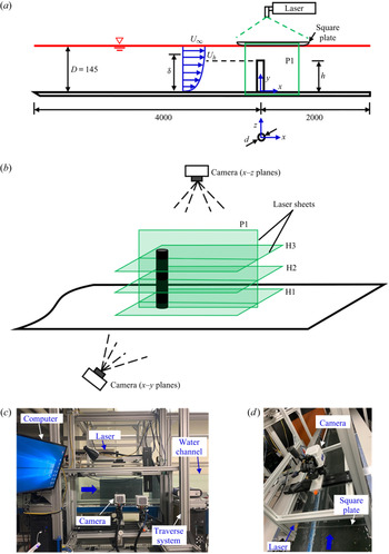
The experiments were carried out in a recirculating open water channel in the Turbulence and Hydraulic Engineering Laboratory (THEL) at the University of Manitoba. The channel has a transparent test section of dimensions 6000 mm long, 600 mm wide (W) and 450 mm deep. The flow was driven by a 30 kW variable-speed drive motor pump through a flow conditioning unit before entering the test section. The flow conditioning unit consists of perforated plates, hexagonal honeycombs, mesh screens of different sizes and has a contraction ratio of 4.88 : 1. Figure 3(a,b) shows the schematic of the flow field and the experimental set-up with a model of the cylinder vertically mounted by means of a screw on the flat acrylic plates lining the entire floor of the test section. The cylinder is a smooth round acrylic rod of diameter, d = 12.7 mm positioned at a streamwise distance of 4000 mm (315d) from the channel's inlet. The centre of the cylinder was carefully aligned with the mid-span of the test section within ±1 mm. The cylinder and the top surface of the bottom plate on which it was mounted were painted with a non-reflective black spray to minimize surface glare from the laser illumination. The incoming boundary layer was tripped with a 16 grit sandpaper strip to facilitate the transition to turbulent flow. The sandpaper has an average roughness height of 1.5 mm, a strip length of 80 mm and spans the entire width of the channel. As shown in figure 3(a), the left-handed Cartesian coordinate system adopted has the origin of the streamwise (x), wall-normal (y) and spanwise (z) directions at the centre of the cylinder on the bottom wall.
(a) Schematic of experimental set-up and nomenclature used in the present study, (b) PIV measurement planes and the arrangements of the camera and laser sheets. Photographs of the set-up of camera and laser for (c) x–y plane and (d) x–z plane measurements. P1 denotes measurements in the x–y plane at the symmetry (z/d = 0) of the cylinder and H1, H2 and H3 denote measurements in the x–z planes. The streamwise velocity at the height of the cylinder is denoted Uh. Not drawn to scale, all dimensions in mm.

To investigate the effects of aspect ratio on the unsteady wake structure of the cylinders, experiments were performed for five different aspect ratios. The aspect ratio, h/d = 7.0 (denoted as AR100) was selected as a reference case and the heights of the four other cylinders were obtained as 10 %, 25 %, 50 % and 75 % of the reference: h/d = 0.7, 1.8, 3.5 and 5.3, respectively. For simplicity, these test cases are denoted as AR10, AR25, AR50 and AR75, respectively. All the experiments were performed with a water depth of D = 145 mm. The maximum blockage ratio based on the frontal area of AR100 and the cross-sectional area of the flow domain is 1.3 %.
The free-stream velocity was kept constant at  ${U_\infty } = 0.436\;\textrm{m}\;{\textrm{s}^{ - 1}}$ and the Reynolds number,
 $Re = {U_\infty }d/\nu = 5540$, where the kinematic viscosity of the working fluid (water) at room temperature (20°C),
 $\nu = {10^{ - 6}}\;{\textrm{m}^2}\;{\textrm{s}^{ - 1}}$. The Froude number
 $({U_\infty }/\sqrt {gD} )$ was 0.37, where g = 9.81 m s−2 is the acceleration due to gravity. The boundary layer thickness of the approach flow (based on the wall-normal location of
 $0.99{U_\infty }$ from the bottom wall) was
 $\delta /d \; = \textrm{8}\textrm{.7}$ (110.5 mm) and the resulting δ/h values were 12.4, 4.8, 2.5, 1.6 and 1.2 for AR10, AR25, AR50, AR75 and AR100, respectively.
2.2. PIV measurements
A planar TR-PIV system supplied by LaVision Inc. was used to measure the velocity fields of the cylinders. Initial measurements were also conducted using the standard double-frame mode of the system to characterize the approach TBL without a cylinder installed in the channel. The flow was seeded with silver coated hollow glass spheres of mean particle diameter, dp = 10 μm and density,  ${\rho _p} = 1400\;\textrm{kg}\;{\textrm{m}^{ - 3}}$. The ability of the particles to follow the flow faithfully was assessed by determining the particle's Stokes number, Sp based on the particle response time, tp and the characteristic temporal scale in the flow, tf as follows:
 \begin{equation}{S_p} = \frac{{{t_p}}}{{{t_f}}} = \frac{{d_p^2({\rho _p} - {\rho _f})}}{{18{\rho _f}\nu {t_f}}},\end{equation}
where ρf is the density of the fluid,  ${t_f} = d/{U_\infty }$. The values of
 ${t_p} = 2.2 \times {10^{ - 6}}$ and
 ${t_f} = 2.9 \times {10^{ - 2}}\;\textrm{s}$ correspond to a Stokes number of
 ${S_p} = 7.6 \times {10^{ - 5}}$, which is orders of magnitude lower than the threshold value of 0.05 (Samimy & Lele Reference Samimy and Lele1991). Therefore, it was concluded that the seeding particles responded faithfully to the changes in direction of the bulk flow.
A dual-cavity high-speed pulsed Nd:YLF laser was used to illuminate the flow field. Each pulse delivered maximum energy of 30 Mj pulse−1 at a sampling frequency (fsp) of 1000 Hz with a wavelength of 527 nm. Using a combination of spherical and cylindrical lenses, the laser sheet was set to 1 mm thickness to reduce the effects of out-of-plane particle motion, which is an important source of error in PIV measurements. The light emitted by the particles were captured using a high-speed 12-bit CMOS camera with a 10 μm pixel pitch and a resolution of 2560 pixels × 1600 pixels. The camera and the laser were mounted on a traverse mechanism which allowed simultaneous streamwise movement of both devices at accurate locations. The data acquisition and post-processing to acquire the instantaneous velocity vectors were performed with the LaVision Inc. software DaVis 10.
For the approach flow, a double-frame measurement was conducted at the mid-span of the channel (x–y plane) without a cylinder installed. The flow field was illuminated from the free surface with the camera capturing the images through the transparent sidewall of the channel (figure 3b,c). Based on a convergence test, 9000 instantaneous image pairs were acquired at a sampling frequency of 4 Hz to obtain statistically independent samples to quantify the turbulent statistics. The field-of-view of the camera was set to 20.5d × 13.0d in the x- and y-directions and the resulting magnification factor was 10 pixels mm−1.
The TR-PIV measurements were performed in the x–y plane (P1) at the symmetry (z/d = 0) of each cylinder as shown in figure 3(b). For the reference case (AR100), additional measurements were conducted in three x–z planes selected at 0.5d from the bottom wall (H1), mid-height (y/d = 3.5) (H2) and 0.5d from the free end (H3) of the cylinder to investigate the unsteady vortex dynamics along the height of the cylinder. In the case of the x–z planes, the laser illumination was from the sidewall and the images were captured with the camera above the channel (figure 3b,d). To minimize free surface distortions of the images captured in the x–z planes, a thin square acrylic plate of length 600 mm (as used in Fang & Tachie Reference Fang and Tachie2019) was positioned beneath the camera and partially immersed in the water to a depth of 2 mm. The leading edge of the plate was rounded to further reduce its influence on the flow. The effect of the plate was investigated using preliminary x–y plane measurements which showed that the boundary layer thickness formed on the plate is very thin (δp = 6.5 mm (0.5d), where δp is based on the wall-normal location of  $0.99{U_\infty }$ from the plate) and the plate has no significant influence on the bulk flow beneath it. Therefore, the plate was used in both the x–y and x–z measurements for consistency.
For both x–y and x–z planes, measurements were acquired with the same field-of-view of the camera which spans approximately  $x/d \in [ - 3.5,13.5]$ and
 $y/d \in [ - 0.5,12.5]$ in the x–y plane and
 $z/d \in [ - 6.5,6.5]$ in the x–z planes. Based on a convergence test, a sample size of 48 000 instantaneous vector frames was acquired in each plane at a sampling frequency of 1000 Hz. This sample size was obtained in eight sets of 6000 images/set. The ratio of the sampling frequency to the spanwise vortex shedding frequency at the mid-height of the tallest cylinder,
 $f_{sp}^\ast{=} {f_{sp}}/{f_s} = 182$ cycles, indicates that the temporal resolution of the measurements is sufficient to capture the unsteady wake characteristics around the cylinders. The number of cycles per each set of images acquired was 33 cycles/set, resulting in a total of 264 cycles for the entire sample size. The total sampling time of T = 48 s corresponds to 1000–1550 characteristic times (d/Uh, where Uh is the streamwise mean velocity at the height of each cylinder) of the flow past the cylinders. This large sampling time was necessary for statistical convergence of the mean velocities, higher-order moments and spectral quantities reported herein.
The PIV images from both the double-frame and time-resolved measurements were post-processed using an adaptive multi-grid cross-correlation algorithm based on multi-pass fast Fourier transform with a 1-D Gaussian peak-fitting function to determine the average particle displacement within an interrogation area. During the experiments, it was ensured that the particle image diameter was approximately 2–4 pixels to minimize pixel-locking-induced errors (Raffel, Willert & Kompenhaus Reference Raffel, Willert and Kompenhaus1998; Adrian & Westerweel Reference Adrian and Westerweel2011). The initial interrogation area was set to 128 pixels × 128 pixels with 50 % overlap and the final size was 32 pixels × 32 pixels with 75 % overlap in each direction. The resulting vector spacing was 0.064d in each direction.
Following Sciacchitano & Wieneke (Reference Sciacchitano and Wieneke2016) and Bendat & Piersol (Reference Bendat and Piersol2010), the uncertainties in the streamwise mean velocity (U), streamwise Reynolds normal stress  $(\overline {{{u^{\prime}}^2}} )$ and Reynolds shear stress
 $( - \overline {u^{\prime}v^{\prime}} )$ for statistically independent or uncorrelated samples can be estimated as
 \begin{equation}{\zeta _U} = \frac{{{\sigma _U}}}{U} = \frac{{{Z_c}}}{{\sqrt N }}\frac{{{u_{rms}}}}{U};\quad {\zeta _{\overline {{{u^{\prime}}^2}} }} = \frac{{{\sigma _{\overline {{{u^{\prime}}^2}} }}}}{{\overline {{{u^{\prime}}^2}} }} = {Z_c}\sqrt {\frac{2}{N}} ;\quad {\zeta _{ - \overline {u^{\prime}v^{\prime}} }} = \frac{{{\sigma _{ - \overline {u^{\prime}v^{\prime}} }}}}{{|{ - \overline {u^{\prime}v^{\prime}} } |}} = {Z_c}\sqrt {\frac{{1 + \rho _{uv}^2}}{{N - 1}}} ;\end{equation}
where σ is the estimated standard error, Zc is the confidence coefficient (e.g. 1.96 for 95 % confidence level), urms is the root mean square of the streamwise velocity fluctuations, ρuv is the correlation coefficient and N is the total number of uncorrelated samples. Analogous expressions can also be written for the other components of the mean velocity and Reynolds stresses. For the double-frame measurement of the approach TBL, the samples are uncorrelated, therefore, (2.2a–c) was used directly with a 95 % confidence coefficient applied. The uncertainty in the streamwise mean velocity, in this case, is less than ±1.0 % across the TBL and the maximum uncertainties in the Reynolds normal stresses and Reynolds shear stress are estimated as ±3.0 % and ±2.3 %, respectively. In the case of the time-resolved measurements of the wake characteristics of the cylinders, the samples are correlated, therefore, it is essential to first determine the effective number of independent samples (Neff) that contribute to statistical convergence using the expression (George, Beuther & Lumley Reference George, Beuther and Lumley1978; Sciacchitano & Wieneke Reference Sciacchitano and Wieneke2016):
 \begin{equation}{N_{eff}} = \frac{T}{{2{T_{int}}}},\end{equation}
where Tint is the integral time scale computed from the temporal autocorrelations of the streamwise velocity fluctuations. Here, the effective number of independent samples were determined at selected locations (x/d = 2 and 8 and  $y/d \in [0.5,8.0]$) in the wake of the two extreme test cases (AR10 and AR100) and the values were used to compute the uncertainties based on (2.2a–c), where N is replaced with Neff. The uncertainty in the mean velocities tends to increase from y-locations near the wall to locations near the free end of the cylinder with values ranging from ±1 % to ±5 %. The uncertainties in the Reynolds normal stresses vary between ±4 % to ±14 %, while those of the Reynolds shear stress vary between ±3 % to ±10 %.
3. Results and discussion
3.1. TBL characterization
The state of the TBL without a cylinder installed is characterized using profiles of the streamwise mean velocity (U) and Reynolds stresses ( $\overline {{{u^{\prime}}^2}} ,\overline {{{v^{\prime}}^2}} \; $ and
 $- \overline {u^{\prime}v^{\prime}} $) as presented in figure 4. The profiles were obtained at the eventual cylinder location at x/d = 0. The pertinent boundary layer parameters are also summarized in table 1. The flow has a relative boundary layer thickness of δ/d = 8.7 and a shape factor of H = 1.41 based on momentum thickness and displacement thickness of θ/d = 1.16 and
 ${\delta ^\ast }/d = 1.63$, respectively. The corresponding Reynolds number based on
 ${U_\infty }$ and θ is
 $R{e_\theta } = 6400$. The inset in figure 4(a) shows that the velocity profile follows the classical log law in the range
 $y/d \in [0.2,4.0]$. The skin friction coefficient,
 ${C_f} = 2{({u_\tau }/{U_\infty })^2}$ (where
 ${u_\tau }$ is the friction velocity obtained from the fitting of the velocity profile on the log law) is
 $2.6 \times {10^{ - 3}}$, and the free-stream streamwise turbulence intensity,
 ${u^{\prime}_{rms}}/{U_\infty } = 1.6\,\%$. The distributions of the mean velocity and Reynolds stresses and the boundary layer parameters agree reasonably well with results reported in previous smooth wall TBL studies at comparable
 $R{e_\theta }$ (Sillero, Jiménez & Moser Reference Sillero, Jiménez and Moser2013; Marusic et al. Reference Marusic, Chauhan, Kulandaivelu, Hutchins, Pollard, Castillo, Danaila and Glauser2017). For example, the shape factor and skin friction coefficient are similar to typical values of
 $H \approx 1.4$ and
 ${C_f} \approx 2.7 \times {10^{ - 3}}$ for
 $R{e_\theta } \in [6000,7000]$ reported in previous studies as compiled by Sillero et al. (Reference Sillero, Jiménez and Moser2013).
Approach TBL profiles. (a) Streamwise mean velocity profile normalized in outer coordinate ( ${U_\infty }$ and d) and logarithmic form (inset),
 ${U^ + } = 1/\kappa (y/d) + B$, where the von Kármán constant, κ = 0.41 and the intercept is set at B = 18. (b) Profiles of Reynolds stresses,
 $\overline {{{u^{\prime}}^2}} ,\overline {{{v^{\prime}}^2}} \; $ and
 $- \overline {u^{\prime}v^{\prime}} $ in outer coordinate. The bars in (a) and vertical dash lines in the inset represent the height of each cylinder relative to the mean velocity profile.

Summary of relevant parameters of the approach TBL.

For bluff bodies fully immersed in a TBL, it is essential to characterize the section of the approach flow that is most likely to affect the flow separation and wake dynamics of the body (Castro Reference Castro1979; Lim, Castro & Hoxey Reference Lim, Castro and Hoxey2007; Fang & Tachie Reference Fang and Tachie2019). Figure 4(a) shows that the height of the cylinders, AR10, AR25 and AR50 are within the logarithmic region while AR75 and AR100 extend into the boundary layer wake region. The heights of the cylinders in wall units,  ${h^ + } = h{u_\tau }/\nu $ are presented in table 2 along with some relevant parameters measured at the cylinder height. The submergence ratio is δ/h = 12.4, 4.8, 2.5, 1.6 and 1.2 for AR10, AR25, AR50, AR75 and AR100, respectively. The streamwise mean velocity at the cylinder height, Uh (hereafter referred to as ‘reduced mean velocity’) ranges from 0.267 to 0.410 m s−1 while the dimensionless mean shear,
 $(\partial U/\partial y{|_h})d/{U_h} \in [0.218,0.040]$ and streamwise turbulence intensity,
 $({u^{\prime}_{rms}}{|_h})/{U_h}(\%) \in [10.2,4.1]$ for AR10 to AR100.
Summary of relevant boundary layer parameters measured relative to the height of the cylinder (h) for each test case, where  ${u^{\prime}_{rms}}$ is the root mean square of the streamwise velocity fluctuations and the subscript h denotes measurement at the cylinder height.

3.2. Flow characteristics over the free end
Prior to discussing the results in the wake of the cylinders, it is important to first examine the influence of aspect ratio and submergence ratio on the separation, attachment and downwash of the separated shear layer over the free end of the cylinders, as presented in this section.
3.2.1. Mean flow and attachment lengths
Figure 5 shows the mean streamlines, and contours of the streamwise mean velocity in an enlarged view of the free end of the cylinders. For each plot, the reverse-flow region (U < 0) is demarcated by the contour line corresponding to the 50 % forward-flow fraction, and the wall-normal distance is measured relative to the top surface of the cylinder  $({y^\ast } = y - h)$ for a better comparison among the various test cases. A distinct reverse-flow region is formed on the top surface of each cylinder and the spiral pattern of the streamlines manifests the presence of flow structures. In particular, the streamlines for AR10 and AR25 reveal the presence of a leading-edge vortex, while the primary and secondary recirculation regions shown in the plots for AR50, AR75 and AR100 reveal the presence of both leading-edge and free-end arch vortices. The leading-edge vortex is suppressed while the arch vortex is enhanced as aspect ratio increases with decreasing submergence ratio, and this has a profound effect on the shape of the reverse-flow region and the angle of deflection of the approach flow over the cylinders. For example, the streamlines in the free stream are essentially horizontal over the reverse-flow region of AR10 and AR25, but the curvature of the streamlines increases as the aspect ratio increases from AR50 to AR100 due to the dominance of the arch vortex. It is noteworthy that the formation of the leading-edge vortex for the smaller aspect ratios (AR10 and AR25) is different from that of AR50–AR100 and the description provided in § 1. This is mainly because of the lack of an arch vortex, therefore, the leading-edge vortex for AR10 and AR25 is the primary structure formed as a result of flow reversal after attachment of the separated shear layer on the top surface of the cylinders. Moreover, AR25 depicts a transitional state for the formation of the free-end arch vortex. For the smallest aspect ratio (AR10), the recirculation region formed behind the cylinder is observed to extend beyond the top surface and this also affects the downwash of the flow over the cylinder.
Contours of streamwise mean velocity at the free end of the cylinder for (a) AR10, (b) AR25, (c) AR50, (d) AR75 and (e) AR100. Superimposed on the contours are with mean streamlines. The red contour line represents the 50 % forward-flow fraction which bounds the reverse-flow region (U < 0). The mean attachment length is denoted as Xr while the maximum height of the reverse-flow region is denoted as Yr.

The streamwise and wall-normal spatial extents of the reverse-flow region are characterized using the mean attachment length, Xr and the maximum height of the reverse-flow region, Yr, respectively. The value of Yr is about 0.045d for AR10 to AR75 but substantially increased to 0.083d for AR100 due to the enhanced arch vortex on the top surface of the cylinder. Figure 6(a,b) examines the effects of aspect ratio and submergence ratio on the attachment length on the top surface of the cylinders. Results from previous studies on circular cylinders are included for comparison. It should be noted that a polynomial curve was fitted to the results from Tsutsui & Kawahara (Reference Tsutsui and Kawahara2006) to improve clarity of the plots. Except for a few scattered data points, the attachment lengths from this study and the previous works indicate a linear increase for  $h/d \in [0.7,8.0]$. In terms of submergence ratio (figure 6b), it is evident that most of the previous studies had the cylinder in a uniform flow or thin boundary layer, where δ/h < 1 and the attachment length is less sensitive to submergence ratio. However, for δ/h > 1, the present results and those of Tsutsui & Kawahara (Reference Tsutsui and Kawahara2006) show a consistent reduction in attachment length as submergence ratio increases. Nonetheless, the present Xr/d values are larger than those of Tsutsui & Kawahara (Reference Tsutsui and Kawahara2006), which may be attributed to the larger aspect ratios used in this study (see figure 6a) and differences in approach flow conditions such as Reynolds number and approach turbulence intensity.
Variation of attachment length on the top surface of the cylinder with (a) aspect ratio, h/d (b) relative boundary layer thickness, δ/h, (c) streamwise mean velocity,  ${U_h}/{U_\infty }$ and mean shear,
 $({ {\partial U/\partial y} |_h})d/{U_h}$ at the cylinder height and (d) streamwise turbulence intensity at the cylinder height,
 $({ {{{u^{\prime}}_{rms}}} |_h})/{U_h}$. In (a,b), the present results are compared with those of previous studies on circular cylinders.

To better understand the controlling parameters that influence the attachment length on the top surface of the submerged cylinders, the relationship between the attachment length and the following dimensionless approach flow parameters:  ${U_h}/{U_\infty }$,
 $(\partial U/\partial y{|_h})d/{U_h}$ and
 $({u^{\prime}_{rms}}{|_h})/{U_h}$ are presented in figure 6(c,d). The plots show that the attachment length increases linearly with increasing reduced mean velocity
 $({U_h}/{U_\infty })$ and decreases as the mean shear
 $((\partial U/\partial y{|_h})d/{U_h})$ increases. On the other hand, increasing the approach turbulence intensity
 $({u^{\prime}_{rms}}{|_h}/{U_h})$ leads to a linear reduction in the attachment length on the cylinders. The variations of the attachment length with the reduced mean velocity and the approach turbulence intensity are consistent with previous studies on separated and reattached flows over surface-mounted bluff bodies in a thick TBL (Essel et al. Reference Essel, Nematollahi, Thacher and Tachie2015; Akon & Kopp Reference Akon and Kopp2016; Nematollahi & Tachie Reference Nematollahi and Tachie2018). In these previous studies, the reduced mean velocity and approach turbulence intensity were evaluated at the height of the body or step. Higher approach turbulence intensity was found to reduce the attachment length on the top surface of the step, while increasing the reduced mean velocity increased the attachment length. The present results suggest that the reduction in attachment length as submergence ratio increases is attributed to the combined effects of the approach flow parameters: Uh,
 ${ {{{u^{\prime}}_{rms}}} |_h}$ and
 ${ {\partial U/\partial y} |_h}$.
3.2.2. Instantaneous flow structures and vortex shedding
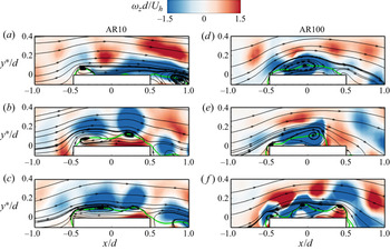
The TR-PIV provides the advantage of carrying out a high frame rate spatio-temporal analysis of the flow structures that are not detectable in the time-averaged flow field. We took advantage of this capability and performed a thorough inspection of the animations of the instantaneous flow fields of each test case. Several different flow structures were observed on the top surface of each cylinder. Herein, we present characteristic snapshots of the instantaneous flow fields that elucidate the important aspects of the dynamic behaviours of the flow structures on the free end of the cylinders. Figure 7 shows snapshots of the instantaneous flow topographies of the two extreme test cases (AR10 and AR100) which reveal the presence of one to three structures on the top surface of each cylinder. Similar qualitative structures were found on the top surface of the other cylinders but are not shown for brevity. In each plot, the instantaneous reverse-flow region is demarcated by the contour line of the 50 % forward-flow fraction and the contours of the instantaneous spanwise vorticity are superimposed on the streamlines. It is clear that the flow features on the top surface of the cylinders are highly intermittent and demonstrate important similarities as well as distinct differences when compared to the time-averaged flow structures (figure 5). For example, the flow topographies shown in figure 7(a) for AR10 and figure 7(e) for AR100 resemble their respective time-averaged topographies while the structures shown in the other snapshots are distinctively different, implying that they occur less frequently.
Characteristic instantaneous flow topographies (streamlines) for the two extreme test cases, AR10 (a–c) and AR100 (d–f) showing minimum to maximum number of vortices on the top surface of the cylinder. The contour of the instantaneous spanwise vorticity is superimposed on each plot. The green contour line represents the 50 % forward-flow fraction which bounds the reverse-flow region.

For each test case, the generation and disintegration of the structures found on the top surface of the cylinder were observed to be erratic as they were highly influenced by the instability introduced by the Kelvin–Helmholtz-like roll-up of the separated shear layers. This instability is evident from the train of spanwise vorticity clusters above the reverse-flow regions and the undulations associated with the stretching and meandering of the vortices. For AR10, the single flow structure formed on the top surface (figure 7a) is often located near the leading edge due to the enhanced approach turbulence intensity and the reduced mean velocity which contracts the reverse-flow region. As aspect ratio increases, the effects of the approach turbulence intensity and reduced mean velocity decrease, which allow the formation of larger structures and longer reverse-flow region (figure 7d–f). The double (figure 7b,e) and triple figure 7(c,f) flow structures are also associated with longer reverse-flow regions and occasional run-off of flow into the near wake behind the cylinders. These structures are formed as a result of the interaction between the reverse flow near the top surface and the separated shear layer over the cylinders.
The periodicity of the vortices shed from the leading edge of the cylinders is evaluated using spectral contours of the streamwise velocity fluctuations in the region immediately above the top surface of each cylinder  $({y^\ast }/d \in [0.0,0.4])$ and at x/d = 0.25 as shown in figure 8. Here, the Strouhal number is defined as
 $S{t_h}\; = {f_s}d/{U_h}$, since the appropriate velocity scale for the submerged cylinders is Uh instead of
 ${U_\infty }$ which is used in previous studies where the cylinders encounter a uniform flow or thin TBL. A salient feature of the spectral contour for each cylinder is the occurrence of multiple peaks, although the dominant peak (i.e. Strouhal number) is detectable in each case. These multiple peaks would imply that the dominant vortex shedding behaviour near the free end of each cylinder is accompanied by other shedding patterns that occur at different frequencies. This is consistent with the results of Hain et al. (Reference Hain, Kahler and Michaelis2008) that showed several vortex shedding frequencies near the free end of a circular cylinder in a thin TBL. As shown in the plots, the dominant vortex shedding occurs at low frequencies and wall-normal locations of approximately 0.07d (AR10) and 0.13d (AR25–AR100) from the top surface of the cylinders. Except for AR50, the Strouhal number based on the dominant frequency decrease with increasing aspect ratio with values of Sth = 0.039, 0.021, 0.011 and 0.005 for AR10, AR25, AR75 and AR100, respectively. For AR50, the Strouhal number based on the dominant frequency is 0.039, however, a secondary Strouhal number can also be found at Sth = 0.018. The reduction in Strouhal number indicate that the vortices shed from the leading edge of the submerged cylinders are more energetic as aspect ratio increases. The Strouhal number for AR25 (h/d = 1.8) when defined based on
 ${U_\infty }$,
 $(St = 0.015)$ agrees well with the value of 0.014 reported by Hain et al. (Reference Hain, Kahler and Michaelis2008) for a circular cylinder of a comparable aspect ratio of h/d = 2.1.
Contours of the energy spectra of the streamwise velocity fluctuations at x/d = 0.25 and over the free end of the cylinder for (a) AR10, (b) AR25, (c) AR50, (d) AR75 and (e) AR100. The vertical dash line indicates the Strouhal number,  $S{t_h}\; = {f_s}d/{U_h}$, while the horizontal dash line marks the corresponding wall-normal location measured relative to the top surface of the cylinder,
 ${y^\ast }/d$.

3.2.3. Flapping motion of the reverse-flow region
Two main approaches have been used in previous investigations to determine the flapping motion (i.e. quasi-periodic expansion and contraction) of the reverse-flow region on a bluff body. These approaches are the temporal variation of the reverse-flow area (Pearson, Goulart & Ganapathisubramani Reference Pearson, Goulart and Ganapathisubramani2013; Graziani et al. Reference Graziani, Kerhervé, Martinuzzi and Keirsbulck2018; Fang & Tachie Reference Fang and Tachie2019) and the coefficients of the first proper orthogonal decomposition mode (Thacker et al. Reference Thacker, Aubrun, Leroy and Devinant2013; Mohammed-Taifour & Weiss Reference Mohammed-Taifour and Weiss2016; Fang & Tachie Reference Fang and Tachie2019). Fang & Tachie (Reference Fang and Tachie2019) used both methods to identify the flapping motion of the reverse-flow regions on a forward—backward-facing step and found that both methods provide consistent results. In this study, we use the temporal variation of the reverse-flow area to characterize the flapping motion of the reverse-flow regions on the cylinders. Following the procedure proposed by Pearson et al. (Reference Pearson, Goulart and Ganapathisubramani2013), the instantaneous area of reverse flow, Ao(t) was determined in a masked region (M) within the field of view as follows:
 \begin{gather}{A_o}(t) = \int_M {\xi (\boldsymbol{u}(x,y,t))\,\textrm{d}x\,\textrm{d}y} ,\end{gather}
 \begin{gather}\xi (p) = \left\{ {\begin{array}{@{}cc} {0,}&{p \ge 0}\\ {1,}&{p \lt 0} \end{array}} \right.,\end{gather}
where u is the instantaneous streamwise velocity,  $\xi (p)$ is the detector function based on the event p, dx and dy represent the vector spacing in the x- and y-directions, respectively. The masked region on the top surface of each cylinder was defined as
 $x/d \in [ - 1,1]$ and
 ${y^\ast }/d \in [0,1]$.
Figure 9(a) shows the effects of aspect ratio and submergence ratio on the normalized mean reverse-flow area (A/d 2). Except for the smallest aspect ratio, AR10 (h/d = 0.7, δ/h = 12.4), the mean reverse-flow area tends to increase with increasing aspect ratio and decreases as submergence ratio increases. The mean reverse-flow area for AR10 is larger than that of AR25 because of the enhanced leading-edge vortex on the top surface of AR10 (see figure 5a). Moreover, the reverse-flow region on AR25 (see figure 5b) appears as a transitional state for the formation of the arch vortex, which will also affect the size of the region.
(a) Variation of the mean reverse-flow area, A/h 2 on the top surface of the cylinder with aspect ratio, h/d. (b) Time sequence of the fluctuating reverse-flow area, A′ normalized by the root-mean-square value, Arms. (c) PDFs of the reverse-flow area A′/h 2. (d) Energy spectra of the reverse-flow area,  ${\emptyset _{AA}}/{h^2}$. The vertical lines correspond to the Strouhal number, Sth ,A. The PDF is normalized such that the maximum value is unity. In (b,d), the profiles are offset with appropriate values to improve clarity of the results presented.

The temporal characteristics of the reverse-flow area are examined in figure 9(b–d). Figure 9(b) shows samples of the time sequence of the fluctuations of the reverse-flow area normalized by the root-mean-square value,  $A^{\prime}/{A_{rms}}$. The enlargement and contraction of the reverse-flow region are clearly demonstrated in the sequence of positive and negative fluctuations. The probability density function (PDF) of A′ (figure 9c) shows that the fluctuations are positively skewed for AR10 and AR25, but the skewness reduces, and the PDF approaches a Gaussian distribution as aspect ratio increases. The positive skewness for AR10 and AR25 means that the instantaneous reverse-flow areas are frequently larger than the mean for the shorter cylinders. However, the taller cylinders exhibit a good balance between expansion and contraction of the instantaneous reverse-flow areas relative to the mean area. These flapping behaviours are further explored using the spectra of these signals shown in figure 9(d). In each test case, the dominant frequency is less pronounced, which suggests that the flapping motion exhibit erratic behaviour over a wide range of frequencies. This may be attributed to the instability generated at the leading edge of the cylinder. Nonetheless, the Strouhal number of the flapping motion of the reverse-flow area is Sth ,A = 0.039 for AR10, AR25 and AR50 and Sth ,A = 0.028 and 0.019 for AR75 and AR100, respectively. For each cylinder, Sth ,A can be detected among the multiple peaks of the energy spectra of the streamwise velocity fluctuations (figure 8), demonstrating a connection between the vortex shedding behaviour and the flapping motion of the reverse-flow region. It is interesting to notice that Sth ,A for AR10 and AR50 agree well with the dominant vortex shedding frequency (Sth = 0.039) at the leading edge of these cylinders.
The flapping motion of the reverse-flow region can be further investigated by examining the relationship between the area, Ao(t) and the streamwise, Xo(t) and wall-normal, Yo(t) extents of the region. The streamwise extent, Xo(t) is defined as the streamwise distance from the leading edge of the cylinder to the farthest location where  $\boldsymbol{u}(x,y,t) \lt 0$ on the top surface of the cylinder, while the wall-normal extent, Yo(t) corresponds to the highest location from the top surface of the cylinder where
 $\boldsymbol{u}(x,y,t) \lt 0$. Figure 10 shows the joint-probability density function (JPDF) of Ao/d 2 paired with Xo/d and Yo/d, respectively. For AR10, the reverse flow is frequently located near the leading edge, with occasional expansion to streamwise locations near the centre
 $({X_o}/d = 0.43)$ and rear end
 $({X_o}/d = 0.73)$ of the cylinder. The height of the reverse-flow region is located at
 ${Y_o}/d = 0.071$ majority of the time, which is higher than the mean height of the region (0.045d). The larger Yo/d and occasional expansion of Xo/d are consistent with the positively skewed PDF of A′ (relative to the mean) for AR10 (figure 9c). The plots for AR10 also demonstrate that the instances where the reverse-flow region disappears are frequent, which is also evident in the case of AR25. As aspect ratio increases, the reverse-flow region is sustained most of the time and the location of frequent occurrence of Xo/d moves closer to the rear end of the cylinder. In particular, the values of Xo/d are centred at 0.57d, 0.62d, 0.77d and 0.79d for AR25, AR50, AR75 and AR100, respectively, which are comparable to the mean attachment lengths. It is interesting to notice that for AR75 and AR100, the height of the region is frequently located at
 ${Y_o}/d = 0.070$, but there is an occasional outburst to a maximum height of
 ${Y_o}/d = 0.130$, in agreement with the quasi-Gaussian PDF of A′ for these test cases (figure 9c). The outburst may be associated with sudden enlargement of the arch vortices, which are dominant on the top surface of these cylinders (see figures 5 and 7).
Comparison of the streamwise (Xo) and wall-normal (Yo) extents of the reverse-flow area on the top surface each cylinder. The wall-normal extent (Yo) is measured relative to the top surface of the cylinder. (a) JPDF of reverse-flow area, Ao and Xo and (b) JPDF of reverse-flow area, Ao and Yo. The JPDF is normalized such that the maximum probability density is unity. The dash horizontal and vertical lines are used to indicate local maximum JPDF locations.

3.3. Flow characteristics in the wake region
This section focusses on the effects of aspect ratio and submergence ratio on the time-averaged and unsteady wake characteristics in the symmetry (x–y) plane of the cylinders.
3.3.1. Mean flow
Figure 11 shows the mean streamlines superimposed on the contours of the wall-normal mean velocity in the symmetry plane of the cylinders. For each test case, the upward deflection (V > 0) of the approach flow over the free end of the cylinder is accompanied by a strong downwash (V < 0) behind the cylinder. In the case of AR10 and AR25, the downwash flow attached to the bottom wall, leading to the formation of a primary recirculation bubble which manifests the presence of an arch vortex (Pattenden et al. Reference Pattenden, Turnock and Zhang2005; Palau-Salvador et al. Reference Palau-Salvador, Stoesser, Fröhlich, Kappler and Rodi2010). As aspect ratio increases beyond AR25, the downwash flow is prevented from attaching onto the bottom wall due to an upwash flow (V > 0) that originate from the base of the cylinder. The clash of the downwash and upwash flows occur at the saddle point (marked as (×)) which is located at  $y/h \approx 0.5$ for AR50, AR75 and AR100. This leads to a bifurcation of the reverse flow, where one part deflects towards the free end and the other part deflect towards the bottom wall. Near the wall, the upwash flow increases as aspect ratio increases, which suggests an enhancement of the base vortices. A trace of the near-wake base vortex is revealed in AR50 and AR75, but the streamlines for AR100 fail to show this flow structure. Similarly, the horseshoe vortices which are expected at the upstream corner of the cylinder and the wall are not resolved in all the test cases.
Mean streamlines in the x–y plane for (a) AR10, (b) AR25, (c) AR50, (d) AR75 and (e) AR100. Superimposed on the streamlines are the contours of the wall-normal mean velocity (V). The red contour line represents the 50 % forward-flow fraction which bounds the reverse-flow region. The green cross mark indicates the saddle point.

Following previous studies (Sumner et al. Reference Sumner, Heseltine and Dansereau2004; Krajnović Reference Krajnović2011; Yauwenas et al. Reference Yauwenas, Porteous, Moreau and Doolan2019), the wake structure for AR10 and AR25 is akin to a dipole while that of AR50, AR75 and AR100 is similar to a quadrupole. The critical aspect ratio in this study,  $h/d\; = \; 3.5$ (AR50) is consistent with values of
 $h/d \in [2,4]$ reported in these previous studies on circular cylinders (Kawamura et al. Reference Kawamura, Hiwada, Hibino, Mabuchi and Kumada1984; Okamoto & Sunabashiri Reference Okamoto and Sunabashiri1992; Sumner et al. Reference Sumner, Heseltine and Dansereau2004). Near the free end of the cylinder, the focus of the recirculation bubble (
 $x/d\; \approx \; 0.9$,
 $y/h\; \approx \; 0.9$) is independent of aspect ratio. This location is also comparable to results of
 $x/d\; \approx \; 0.9$ and
 $y/h\; \approx \; 0.8$ reported by Palau-Salvador et al. (Reference Palau-Salvador, Stoesser, Fröhlich, Kappler and Rodi2010) for circular cylinders of h/d = 2.5 and 5.0 in a thin TBL.
Contours of the streamwise mean velocity are presented in figure 12. The mean velocity vectors with appropriate spacing in the streamwise direction are superimposed on the contours to depict the evolution of the mean flow. The plots show that most of the perturbations in the TBL caused by the presence of the cylinders are confined to the region below the contour line of U = Uh. The features of the wake behind the cylinders (as depicted by the contour line of  $U/{U_\infty } = 0.5$) become more complex as aspect ratio increases due to the concurrent interactions of the downwash and upwash flow and the redevelopment of the TBL on the wall.
Contours of the streamwise mean velocity (U) for (a) AR25, (b) AR50, (c) AR75 and (d) AR100. Superimposed are the velocity vectors. The red solid contour line represents the 50 % forward-flow fraction which bounds the reverse-flow region. The green solid line and blue dash line represent  $U/{U_\infty } = 0.5$ and
 $U/{U_h} = 1$, respectively.

The reverse-flow region behind the FWMCs is largely influenced by the aspect ratio. The maximum backflow velocity in this study, for example, increased from  $- 0.2{U_\infty }$ to
 $- 0.3{U_\infty }$ as aspect ratio increased from AR10 to AR100. To perform more detail investigations on the effects of aspect ratio on the statistical properties of the reverse-flow region, the distributions of the streamwise extent (Lr), the mean area (A) and root mean square of the fluctuations of the area (Arms) of the reverse-flow region are presented in figure 13. The value of Lr is determined as the streamwise distance from the rear end of the cylinder (x/d = 0.5) to the furthest point on the contour line of the 50 % forward-flow fraction. In figure 13(a), the results of Lr/d reported in previous circular and square FWMC studies (Wang & Zhou Reference Wang and Zhou2009; Bourgeois et al. Reference Bourgeois, Sattari and Martinuzzi2011; Rostamy et al. Reference Rostamy, Sumner, Bergstrom and Bugg2012) are included for comparison. It should be noted that all the previous studies were conducted with submergence ratios,
 $\delta /h \lt 1$. In all cases, the reverse-flow region for the FWMCs are more elongated compared to that of 2D circular cylinders
 $({L_r}/d \approx 0.6)$ in a sub-critical Reynolds number regime (Cantwell & Coles Reference Cantwell and Coles1983; Rodríguez et al. Reference Rodríguez, Lehmkuhl, Chiva, Borrell and Oliva2015). The present results show a gradual increase in Lr/d from 1.3 to 2.3 as aspect ratio increases from
 $h/d\; = \; 0.7$ (AR10) to 7.0 (AR100). Although the results of the previous studies also show a consistent increase in Lr/d for
 $h/d \in [3.0,7.0]$, the maximum value (Lr/d = 3.3) at h/d = 7.0 is 43 % larger than that of the present study. This difference may suggest that the submergence of the cylinder in the TBL suppresses streamwise expansion of the reverse-flow region. Nonetheless, when Lr/d = 3.3 at h/d = 7.0 is excluded, the Lr/d values for all the studies asymptote at 2.4 ± 0.2 for
 $h/d \in [4.0,11.0]$. In figure 13(b), the mean area of the reverse flow behind each cylinder was computed based on (3.1) and (3.2). A mask of
 $x/d \in [0.5,5.0]$ and
 $y/d \in [0.0,8.0]$ was used for all the test cases. Both the mean and fluctuations of the area of the reverse flow increase monotonically with increasing aspect ratio. However, the slope of the mean area profile (kA = 1.60) is larger than that of the fluctuations
 $({k_{{A_{rms}}}} = 0.22)$. When the results in figure 13 are plotted in terms of δ/h, the streamwise extent, mean and fluctuations of the area of the reverse flow were found to decrease with increasing submergence ratio.
Variation of (a) streamwise extent of reverse-flow region, Lr and (b) mean reverse-flow area, A and root mean square of the fluctuations of the reverse-flow area, Arms behind the cylinder with aspect ratio, h/d.

The streamwise evolution of the wake flow behind a bluff body can be characterized using the maximum velocity difference,  $\Delta U = {U_{max}} - {U_{min}}$, where Umax and Umin are the local maximum and minimum streamwise mean velocities, respectively. For the FWMCs, the value of Umin beyond the reverse-flow region is zero at the wall, although the wake may still persist. Therefore, we defined ΔU for the FWMCs as
 $\mathrm{\Delta }U = {U_{max}} - {U_i}$, where
 ${U_i} = {U_{min}}$ in the reverse-flow region and Ui is the local minimum velocity outside the thin boundary layer that is redeveloping on the wall. Figure 14(a,b) shows the distributions of ΔU normalized by
 ${U_\infty }$ and Uh. The profiles increase sharply to a peak value at the location of the maximum backflow velocity, followed by a gradual decay with increasing streamwise distance. However, the decay of the wake is curtailed more quickly as aspect ratio decreases due to the dominance of the redeveloping TBL. In figure 14(b), it is observed that the use of Uh as the velocity scale results in a good collapse of the profiles beyond the local peak values. These profiles follow an exponential distribution given as
 \begin{equation}\Delta U/{U_h} = 2.6\,\textrm{exp}( - 0.5(x/d)) + 0.5.\end{equation}
Streamwise development of velocity defect; (a)  $\Delta U/{U_\infty }$ and (b)
 $\Delta U/{U_h}$ and (c) vorticity thickness,
 ${\delta _\omega }$ in the wake region of the cylinders.

The vorticity thickness is an important parameter used to characterize the growth rate of separated shear layers and mixing layers (Brown & Roshko Reference Brown and Roshko1974; Simpson Reference Simpson1989). Traditionally, the vorticity thickness is defined as  ${\delta _\omega } = \Delta U/({ {\partial U/\partial y} |_{max}})$, where
 ${ {\partial U/\partial y} |_{max}}$ is the local maximum value in the mean shear profile. Here, the structure of the shear layers behind the FWMCs is more complicated as the profiles of
 $\partial U/\partial y$ exhibit multiple (1–3) peaks which represent the separated shear layers (i.e. downwash and upwash) and the thin boundary layer redeveloping on the bottom wall. The peaks of the separated shear layers decrease and eventually diminish further downstream while the peak near the bottom wall increases due to the redevelopment of the TBL. Therefore, to avoid any bias in the distributions of
 ${\delta _\omega }$ arising from the elevated mean shear on the wall, we carefully defined
 ${ {\partial U/\partial y} |_{max}}$ as the local maximum value of mean shear in the separated shear layers. As shown in figure 14(c), the vorticity thickness increases linearly with streamwise distance and the extent of the linear growth is influenced by the persistence of the separated shear layers in each test case. The growth rate,
 $\textrm{d}{\delta _\omega }/\textrm{d}x = 0.50$ is independent of aspect ratio, although the vorticity thickness for AR10 is reduced compared to the other test cases. Nonetheless, this growth rate is 34%–78 % higher than values (0.11–0.33) reported for plane mixing layers (Brown & Roshko Reference Brown and Roshko1974), forward- and backward-facing steps (Jovic Reference Jovic1996; Essel & Tachie Reference Essel and Tachie2015; Fang & Tachie Reference Fang and Tachie2019) and surface jets (Rahman et al. Reference Rahman, Tay, Essel and Tachie2018; Essel, Roussinova & Balachandar Reference Essel, Roussinova and Balachandar2020). For AR75 and AR100, it is observed that the profiles exhibit a second stage of growth where the vorticity thickness decreases gradually to nearly constant values further downstream.
3.3.2. Reynolds stresses and production
Figure 15 shows the contours of the Reynolds stresses  $(\overline {{{u^{\prime}}^2}} ,\overline {{{v^{\prime}}^2}} \;\textrm{and}\; - \overline {u^{\prime}v^{\prime}} )$ for AR25, AR50 and AR100. The contours for AR10 (not shown) are qualitatively similar to those of AR25 since these test cases have a similar wake structure (dipole). On the other hand, the contours for AR75 are qualitatively similar to AR100, therefore, not shown for brevity. The Reynolds stresses generally increases with increasing aspect ratio, which is consistent with previous FWMC studies (Wang & Zhou Reference Wang and Zhou2009; Rostamy et al. Reference Rostamy, Sumner, Bergstrom and Bugg2012). It is also interesting to observe that the magnitude of the streamwise Reynolds normal stress
 $(\overline {{{u^{\prime}}^2}} )$ is less than the wall-normal Reynolds normal stress
 $(\overline {{{v^{\prime}}^2}} )$. Although this observation signifies large-scale anisotropy, it is contrary to the norm in many simple turbulent shear flows where
 $\overline {{{u^{\prime}}^2}} $ is larger than the other components (
 $\overline {{{v^{\prime}}^2}} $ and spanwise Reynolds normal stress,
 $\overline {{{w^{\prime}}^2}} $). For the dipoles (figure 15a,d,g), the Reynolds stresses
 $(\overline {{{u^{\prime}}^2}} ,\overline {{{v^{\prime}}^2}} \;\textrm{and}\; - \overline {u^{\prime}v^{\prime}} )$ emanating from the downwash flow attach onto the bottom wall and combine with the stresses in the redeveloping TBL. The quadruples (AR50 and AR100), on the other hand, exhibit two regions of concentrated Reynolds stresses per the downwash and upwash flows. However, the Reynolds stresses in the downwash flow are more pronounced and persist further downstream than their counterparts in the upwash flow. This is attributed to enhanced entrainment of free-stream fluid into the downwash flow.
Contours of streamwise (a–c) and wall-normal (d–f) Reynolds normal stresses and Reynolds shear stress (g–i) in the x–y plane for AR25 (first column), AR50 (second column) and AR100 (third column). The black solid contour line represents the 50 % forward-flow fraction which bounds the reverse-flow region. The red dash lines represent  $U/{U_h} = 1$.

Figure 16 compares the streamwise development of the maximum Reynolds stresses behind the cylinders. The distributions of the maximum  $\overline {{{v^{\prime}}^2}} $ show a consistent increase with increasing aspect ratio. The maximum
 $\overline {{{u^{\prime}}^2}} $, on the other hand, exhibits inconsistencies, although the peaks are usually enhanced as aspect ratio increases. The peak values of the Reynolds normal stresses provide a measure of the vortex formation length, Lv (Gerrard Reference Gerrard1966; Cantwell & Coles Reference Cantwell and Coles1983; Szepessy & Bearman Reference Szepessy and Bearman1992; Rodríguez et al. Reference Rodríguez, Lehmkuhl, Chiva, Borrell and Oliva2015) defined as the streamwise distance from the rear end of the cylinder (x/d = 0.5) to the peak location. Here, the variation of Lv/d with aspect ratio behaves similarly as Lr/d (figure 13a) with values that increases from Lv/d = 1.0–2.0 for AR10 to AR100. The difference (1d) between the test cases would imply that the vortex formation process behind the cylinders is less sensitive to the effects of aspect ratio. This is consistent with results of previous FWMC studies (Wang & Zhou Reference Wang and Zhou2009; Palau-Salvador et al. Reference Palau-Salvador, Stoesser, Fröhlich, Kappler and Rodi2010; Rostamy et al. Reference Rostamy, Sumner, Bergstrom and Bugg2012).
Streamwise development of maximum (a) streamwise and (b) wall-normal Reynolds normal stresses, (c) stress ratio,  $\overline {{{v^{\prime}}^2}} /\overline {{{u^{\prime}}^2}} $ and (d) maximum Reynolds shear stress behind the cylinders.

Unlike AR50–AR100 where the  $\overline {{{u^{\prime}}^2}} $ distribution beyond the peak decrease with streamwise distance, the profiles for AR10 and AR25 tends to plateau at x/d = 3.5 and 5.5, respectively. The plateau of the distribution is due to the enhanced
 $\overline {{{u^{\prime}}^2}} $ in the redeveloping boundary layer near the wall for the shorter cylinders. The stress ratio,
 $\overline {{{v^{\prime}}^2}} /\overline {{{u^{\prime}}^2}} $ (figure 16c) demonstrate two forms of anisotropy in the wake region of the cylinders. The first refers to the section where
 $\overline {{{v^{\prime}}^2}} /\overline {{{u^{\prime}}^2}} \lt 1$ (i.e.
 $\overline {{{u^{\prime}}^2}} \gt \overline {{{v^{\prime}}^2}} $) and the second section is an opposite trend where
 $\overline {{{v^{\prime}}^2}} /\overline {{{u^{\prime}}^2}} \gt 1$ (i.e.
 $\overline {{{u^{\prime}}^2}} \lt \overline {{{v^{\prime}}^2}} $). For AR10, the anisotropy is predominantly of the first form,
 $\overline {{{u^{\prime}}^2}} \gt \overline {{{v^{\prime}}^2}} $ with the tail of the profile departing from the isotropy mark
 $(\overline {{{v^{\prime}}^2}} /\overline {{{u^{\prime}}^2}} = 1)$ for x/d ≥ 2.0. The increase in anisotropy with streamwise distance for AR10 is attributed to the enhanced mean shear
 $(\partial U/\partial y)$ in the redeveloping boundary layer near the wall, which contribute significantly to the production of
 $\overline {{{u^{\prime}}^2}} $
 $( - \overline {u^{\prime}v^{\prime}} \partial U/\partial y)$ near the wall. For AR25–AR100, the profiles exhibit both forms of anisotropy. In the region,
 $x/d \in [0.0,\; 1.2]$,
 $\overline {{{u^{\prime}}^2}} \gt \overline {{{v^{\prime}}^2}} $ due to the large mean shear in the separated shear layer over the free end of the cylinder, which enhances
 $\overline {{{u^{\prime}}^2}} $. For x/d > 1.2, the anisotropy flips to
 $\overline {{{u^{\prime}}^2}} \lt \overline {{{v^{\prime}}^2}} $ and rapidly increases to a maximum value at about x/d = 2.0. Further downstream, the Reynolds stresses approaches isotropy for AR50–AR100, however, AR25 shows another switch at x/d ≥ 6.0 back to
 $\overline {{{u^{\prime}}^2}} \gt \overline {{{v^{\prime}}^2}} $. The second switch for AR25 is because of the stronger influence of the mean shear near the wall on the production of
 $\overline {{{u^{\prime}}^2}} $. The region where
 $\overline {{{u^{\prime}}^2}} \lt \overline {{{v^{\prime}}^2}} $ requires further investigation to understand this unique behaviour. For the Reynolds shear stress (figure 16d), the maximum values occur in the downwash flow, therefore, the distributions of the maximum
 $- \overline {u^{\prime}v^{\prime}} $ are positive throughout the wake region. Except for AR10, the maximum
 $- \overline {u^{\prime}v^{\prime}} $ is independent of aspect ratio in the region,
 $x/d \in [0.5,5.0]$, but further downstream,
 $- \overline {u^{\prime}v^{\prime}} $ tends to increase as aspect ratio increases.
As noted above, the anisotropy of the Reynolds stresses for AR25–AR100 show an interesting pattern where  $\overline {{{u^{\prime}}^2}} $ is less than
 $\overline {{{v^{\prime}}^2}} $. We provide further insight into this phenomenon by examining the production terms of
 $\overline {{{u^{\prime}}^2}} $ and
 $\overline {{{v^{\prime}}^2}} $, denoted as Puu and Pvv, respectively. At the symmetry plane, the gradient
 $\partial ({\cdot} )/\partial z \approx 0$, therefore the production terms for
 $\overline {{{u^{\prime}}^2}} $ and
 $\overline {{{v^{\prime}}^2}} $ reduces to
 \begin{gather}{P_{uu}} = \underbrace{{ - 2\overline {{{u^{\prime}}^2}} \partial U/\partial x}}_{{{P_{uu - n}}}}\underbrace{{ - 2\overline {u^{\prime}v^{\prime}} \partial U/\partial y}}_{{{P_{uu - s}}}},\end{gather}
 \begin{gather}{P_{vv}} = \underbrace{{ - 2\overline {{{v^{\prime}}^2}} \partial V/\partial y}}_{{{P_{vv - n}}}}\underbrace{{ - 2\overline {u^{\prime}v^{\prime}} \partial V/\partial x}}_{{{P_{vv - s}}}},\end{gather}
where  ${P_{uu - n}}$ and
 ${P_{uu - s}}$ denote the contributions of the normal stress and shear stress, respectively, to the net Puu. Similarly, the total Pvv is decomposed into contributions from the normal stress
 $({P_{vv - n}})$ and the shear stress
 $({P_{vv - s}})$. Here, the reference test case (AR100) is used to assess the individual production terms as shown in figure 17. A striking feature in the Puu contour (figure 17a) is the negative production of
 $\overline {{{u^{\prime}}^2}} $ (energy sink) along the boundary of the reverse-flow region. This energy sink is due to the contribution of
 ${P_{uu - n}}$ (figure 17b), which is suppressed near the free end by the dominance of
 ${P_{uu - s}}$ (figure 17c) in the separated shear layer over the cylinder. Near the boundary of the reverse-flow region,
 $\partial U/\partial x$ is significantly enhanced because of the large velocity difference and this in turn contributes to the high energy sink
 $({P_{uu - n}})$ that surpasses the main energy source of
 $\overline {{{u^{\prime}}^2}} $
 $({P_{uu - s}})$ in that region. From figure 17(d–f), it is evident that Pvv is essentially positive with most of the energy source derived from
 ${P_{vv - n}}$. The contribution of the shear stress term,
 ${P_{vv - s}}$ to the net production is negligibly small.
Contours of the production terms of the Reynolds normal stresses (a) Puu, (b)  ${P_{uu - n}}$, (c)
 ${P_{uu - s}}$, (d) Pvv, (e)
 ${P_{vv - n}}$ and (f)
 ${P_{vv - s}}$ for AR100.

The above analysis, based on figures 16 and 17, provides an indication that the anisotropy,  $\overline {{{u^{\prime}}^2}} \lt \overline {{{v^{\prime}}^2}} $ is due to the negative production of
 $\overline {{{u^{\prime}}^2}} $. As will be shown later, the magnitude of
 $\overline {{{w^{\prime}}^2}} $ (see figure 23) is also larger than
 $\overline {{{v^{\prime}}^2}} $ and
 $\overline {{{u^{\prime}}^2}} $. This would imply that most of the energy in
 $\overline {{{u^{\prime}}^2}}$ near the boundary of the reverse-flow region (figure 15a,b) is derived from the pressure-strain term which redistributes energy from the other components (
 $\overline {{{v^{\prime}}^2}} $ and
 $\overline {{{w^{\prime}}^2}} $) to overcome the deficit in
 $\overline {{{u^{\prime}}^2}} $. Since
 $\overline {{{w^{\prime}}^2}} $ is the largest, it is expected to be the primary donor in this energy redistribution.
3.3.3. Flapping motion of the reverse-flow region
Characteristic snapshots of the instantaneous flow fields behind the cylinders for AR10, AR50 and AR100 are presented in figure 18. The instantaneous streamlines bear resemblance to the time-averaged flow topography for each test case, although the near-wake base vortex at the corner of AR50 and the wall is more distinct here. In general, the instantaneous reverse-flow region has irregular boundaries compared to that of the time averaged, and exhibit small disjoint patches, especially for larger aspect ratios. The flapping motion of the reverse-flow area, Ao(t) was investigated by summing all the regions of u < 0 (3.1) and (3.2) behind each cylinder ( $x/d \in [0.5,5.0]$ and
 $y/d \in [0.0,8.0]$).
Characteristic instantaneous flow topographies (streamlines) in the x–y plane behind the cylinder for (a) AR10, (b) AR50 and (c) AR100. Superimposed on the streamlines are the instantaneous streamwise velocity, u.

Figure 19 compares the temporal distributions and scales of the reverse-flow area for all the test cases. As shown in figure 19(a), the temporal fluctuations of the reverse-flow area demonstrate the enlargement and contraction of the region for each test case. The PDFs of the fluctuations (figure 19b) show a Gaussian distribution for all the test cases, except for AR100 which is negatively skewed and exhibits two off-centre peaks.
(a) Time sequence of the fluctuating reverse-flow area behind the cylinder, A′ normalized by the root-mean-square value, Arms. (b) PDFs of the reverse-flow area A′/h 2. (c) Temporal autocorrelations of reverse-flow area, RAA. (d) Pre-multiplied frequency spectra of the reverse-flow area,  $f{\emptyset _{AA}}$ behind each cylinder. In (a,d), the profiles are offset with appropriate values to improve clarity of the results presented.

The temporal scales and the dominant flapping frequencies are determined using the temporal autocorrelations (RAA), and pre-multiplied frequency spectra of the fluctuations of the reverse-flow area shown in figure 19(c,d). The autocorrelations (RAA) show a consistent increase in the temporal scale of the reverse-flow area as aspect ratio increases. The temporal integral scale is measured as the area under RAA(t) from the self-correlation point to the point where the tail of the curve first crosses zero for each test case. The first location where the tail crosses zero was chosen for consistency as the tails for the various test cases tend to fluctuate about the zero mark with increasing time sequence. The temporal integral scale is tUh/d = 1.4, 2.7, 5.2, 6.3 and 11.6 for AR10, AR25, AR50, AR75 and AR100, respectively. In figure 19(f), the frequency spectra indicate two dominant flapping frequencies for AR100 (Sth ,A = 0.012 and 0.023) similar to the double peaks of the PDF of A′ (figure 19b), and a single dominant frequency for AR50 (Sth ,A = 0.026) and AR75 (Sth ,A = 0.017). For AR10 and AR25, the dominant frequencies are less distinct, which may be due to the suppression of the spanwise vortices as aspect ratio decreases.
Figure 20 examines the effects of aspect ratio on the JPDF of the instantaneous area, Ao(t) and the streamwise extent, Lo(t) of the reverse-flow region behind the cylinders. The streamwise extent, Lo(t) is determined as the streamwise distance from the rear end of the cylinder (x/d = 0.5) to the farthest point on the instantaneous reverse-flow area. For AR10, the flapping of the reverse flow in the streamwise direction is extremely minimal, which is consistent with the lack of distinct dominant frequency in the spectra distribution. As the aspect ratio increases, the flapping motion becomes more pronounced as evident from the enlargement of the JPDFs. The streamwise extent of the JPDF contours of Ao(t) and Lo(t) can be used to estimate the flapping length (Lfl) of the boundary of the reverse-flow region. Here, the two furthest points on the 0.6 contour level of the JPDFs were used, which showed that the flapping length increased from Lfl/d = 0.4 to 0.8 as aspect ratio increased from AR10 to AR25 for the dipoles. In the case of the quadruples, the flapping length increased to an asymptotic value of Lfl/d = 1.5 ± 0.1 for these test cases.
JPDF of reverse-flow area, Ao and streamwise extent of the reverse-flow area, Lo behind each cylinder. The plus sign represents the centre of the JPDF. The JPDF is normalized such that the maximum probability density is unity.

3.3.4. Spatio-temporal evolution of the vortical structures
The evolution of the vortical structures (spanwise, tip and base vortices) and their interactions behind the FWMCs can be investigated using temporal histories of the in-plane (spanwise) vorticity,  ${\omega _z}(x,t)$. Figure 21 shows snapshots of the instantaneous spanwise vorticity for AR25, AR50 and AR100 and the corresponding temporal histories extracted at x/d = 1 and 5 are presented in figure 22. For each test case, the vortices shed from the free end (figure 21) are swept downward by the downwash flow to interact with the other vortices in the wake. The downward inclination of these vortices has also been observed in previous studies (Palau-Salvador et al. Reference Palau-Salvador, Stoesser, Fröhlich, Kappler and Rodi2010; Krajnović Reference Krajnović2011). Traces of the spanwise vortices originating from the Kelvin–Helmholtz instability along the sides can be observed immediately behind the cylinders for AR50 and AR100. These spanwise vortices are larger near the boundary of the reverse-flow region because of the roll-up of the shear layers and the alternating vortex shedding process. Near the wall, it is observed that the vortices for AR50 and AR100 are convected further away from the wall when compared with those of AR10. This observation is attributed to the upwash flow which is present in the wake of the quadruples.
Contours of instantaneous spanwise vorticity in the wake region of (a) AR25, (b) AR50 and (c) AR100. The green dash contour lines represent U/Uh = 1, while the black solid lines represent the boundary of the mean reverse-flow region for each test case.

Spatio-temporal distributions of spanwise vorticity extracted at x/d = 1 (L1, first column) and x/d = 5 (L2, second column) for AR25 (a,b), AR50 (c,d) and AR100 (e,f).

The temporal histories of the vortices through the reverse-flow region (figure 22a,c,e) indicate that the shedding behaviour near the free end is inherently different from those along the lower span of the cylinders. In particular, the vortices near the trailing edge of the cylinders are shed discretely, while those beneath are depicted as long streaky structures. This phenomenon of different shedding behaviour along the entire span of a cylinder has been observed in previous FWMC studies (Okamoto & Yagita Reference Okamoto and Yagita1973; Farivar Reference Farivar1981; Lee Reference Lee1997; Yauwenas et al. Reference Yauwenas, Porteous, Moreau and Doolan2019), and is often referred to as cellular shedding. This cellular shedding behaviour will be investigated in detail using the tallest cylinder (AR100) in § 3.4.2. The plots also show that the vorticity clusters are predominantly negative for AR25 due to the downwash flow, but as aspect ratio increases, the negative vorticity clusters in the lower span of the cylinder are interspaced with increasing number of positive clusters. The increased number of positive clusters is attributed to the influence of the upwash flow from the wall and the alternating vortex shedding behaviour along the span of the cylinder. In figure 22(b,d,f), the disorganized distributions of the vortices passing through x/d = 5 demonstrate the breakdown of the structures as the wake flow interacts with the TBL. Moreover, the vortices near the free end of each cylinder disappear. This is attributed to the downward sweep of the vortices, and their disintegration as they collide with larger ones along the mid-span of the cylinder.
3.4. Spanwise wake structure and vortex shedding
With the effects of aspect ratio on the unsteady wake characteristics of the submerged FWMCs established in §§ 3.2 and 3.3, this section focuses on the flow fields in the x–z planes (H1, H2 and H3) of the reference cylinder (AR100).
3.4.1. Mean velocities and turbulence statistics
Figure 23 presents the contours of the streamwise and spanwise mean velocities in the x–z planes (H1, H2 and H3) of AR100. The mean streamlines are superimposed on the contours of the spanwise mean velocity to reveal the flow pattern. Also shown on the plots are the boundary of the reverse-flow region, and the contour line corresponding to U/Uh = 0.5 used to depict the wake pattern. It is important to recall that the plane, H2 is at the mid-height of the cylinder while H1 and H3 are located at 0.5d from the bottom wall and the free end of the cylinder, respectively. In figure 23(a,c,e), it is interesting to notice that the wake pattern varies across the three planes, demonstrating the strong influence of the base vortices at H1, the spanwise vortices at H2 and the tip vortices at H3. At H3, the section of the reverse-flow region is absent due to the effects of the downwash flow. The spanwise mean velocity shows that the entrainment of the surrounding TBL into the wake is more intense near the ends of the cylinder (figure 23b,f) than at the mid-span (figure 23d). This is consistent with the suppressed wake near the free end and the bottom wall (figure 23a,e) compared with the section of the wake at the mid-span of the cylinder (figure 23c).
Contours of the streamwise (a,c,e) and spanwise (b,d,f) mean velocities in the x–z planes, H1, H2 and H3 of AR100. The mean streamlines are superimposed on the spanwise mean velocity contours. The solid red contour line on the contours represents the 50 % forward-flow fraction which bounds the reverse-flow region, while the black dashed lines on the streamwise mean velocity contour represent U/Uh = 0.5.

Contours of the Reynolds stresses  $(\overline {{{u^{\prime}}^2}} ,\overline {{{w^{\prime}}^2}} \;\textrm{and}\; - \overline {u^{\prime}w^{\prime}} )$ and the wall-normal vorticity fluctuations
 $({\omega _{y,rms}})$ are presented in figures 24 and 25. Both
 $\overline {{{u^{\prime}}^2}} $ and
 $- \overline {u^{\prime}w^{\prime}} $ are enhanced in the separated shear layers while
 $\overline {{{w^{\prime}}^2}} $ and
 ${\omega _{y,rms}}$ are more intense within the wake behind the cylinder. The anisotropy of the Reynolds stresses is also strong in the spanwise plane as the magnitude of
 $\overline {{{w^{\prime}}^2}} $ is larger than
 $\overline {{{u^{\prime}}^2}} $. Moreover,
 $\overline {{{u^{\prime}}^2}} $ in the spanwise plane is more intense than in the symmetry plane, and
 $- \overline {u^{\prime}w^{\prime}} $ is larger than
 $- \overline {u^{\prime}v^{\prime}} $ (see figure 15). The plots also show that these turbulence statistics in the spanwise planes are reduced towards the ends of the cylinder and the effect is more pronounced near the bottom wall which is explained by the suppression of the spanwise vortex shedding as the ends of the cylinder are approached. The present results agree with previous studies on finite wall-mounted circular cylinders (Parnaudeau et al. Reference Parnaudeau, Carlier, Heitz and Lamballais2008; Palau-Salvador et al. Reference Palau-Salvador, Stoesser, Fröhlich, Kappler and Rodi2010).
Contours of the streamwise (a,c,e) and spanwise (b,d,f) Reynolds normal stresses in the x–z planes, H1, H2 and H3 of AR100. The solid green contour line on the contours represents the 50 % forward-flow fraction which bounds the reverse-flow region, while the black dashed lines represent U/Uh = 0.5.

Contours of the Reynolds shear stress (a,c,e) and wall-normal vorticity fluctuations (b,d,f) in the x–z planes, H1, H2 and H3 of AR100. The solid green contour line on the contours represents the 50 % forward-flow fraction which bounds the reverse-flow region, while the black dashed lines represent U/Uh = 0.5.

3.4.2. Cellular vortex shedding
Cellular shedding is an interesting phenomenon observed along the span of circular FWMCs, but the parameters influencing the occurrence of this behaviour is still not well understood. Okamoto & Yagita (Reference Okamoto and Yagita1973) and Farivar (Reference Farivar1981) investigated the variation of Strouhal number along the span of a circular cylinder and found a reduction in Strouhal number with increasing wall-normal distance from the base to the free end of the cylinder. Although the results of Okamoto & Yagita (Reference Okamoto and Yagita1973) showed a gradual decrease with wall-normal distance for cylinders of h/d = 7, 9 and 12, Farivar (Reference Farivar1981) observed the reduction in a stepwise manner for cylinders of h/d = 10, 11 and 12.5, thereby suggesting a cellular structure of the vortex shedding behind the cylinders. This cellular structure, however, contradicts the one-cell uniform vortex shedding model proposed by Krajnović Reference Krajnović2011 (figure 2a). Moreover, previous investigations have shown that the cellular shedding disappears for h/d < 7 (Okamoto & Sunabashiri Reference Okamoto and Sunabashiri1992; Lee Reference Lee1997; Porteous et al. Reference Porteous, Moreau and Doolan2014), while Sakamoto & Oiwake (Reference Sakamoto and Oiwake1984) and Sumner et al. (Reference Sumner, Heseltine and Dansereau2004) suggested that larger  $\delta /h$ may suppress the cellular shedding behaviour even for h/d > 7. In this study, we perform further investigation of this phenomenon using the spanwise planes of AR100 (h/d = 7).
Figure 26 shows spanwise spectral contours of the streamwise velocity fluctuations extracted at x/d = 3 in the planes, H1, H2 and H3 for AR100. These contours are accompanied by spectral profiles obtained at the spanwise location of the dominant frequency in each plane. At the mid-height of the cylinder (H2), the energy spectra contour shows pronounced vortex shedding peak that is concentrated at a distinct dominant frequency and centred at z/d = −0.8. However, the strength of the vortex shedding reduces, and the peak occupies a wider frequency band as the free end and the bottom wall are approached. Moreover, the intense energy region moves closer to the cylinder for H1 and H3 with centres at z/d = −0.45 and −0.36, respectively. These observations demonstrate the damping effects of the downwash and upwash flow on the strength of the vortex shedding behaviour. It is evident that the Strouhal number is not constant in the three planes but decreases towards the free end. In particular, the Strouhal number near the bottom wall is approximately Sth = 0.20, but decreased to 0.17 at the mid-height and 0.02 near the free end. When the Strouhal number is defined based on the free-stream velocity, the values of St = 0.16 and 0.18 for H1 and H2, respectively, are in good agreement with  $St \in [0.15,0.18]$ usually reported for circular FWMCs of h/d < 10 (Porteous et al. Reference Porteous, Moreau and Doolan2014). The present results at H1 and H2 agree well with the variation of Strouhal number reported by Farivar (Reference Farivar1981), however, the Strouhal number near the free end (St = 0.02) is significantly lower than the average value of 0.07 observed in Farivar (Reference Farivar1981) and Kitagawa, Fujino & Kimura (Reference Kitagawa, Fujino and Kimura1999). Nonetheless, the present study demonstrates that cellular shedding behaviour is not only confined to FWMCs in uniform flow or thin TBL but may also occur in submerged FWMCs
 $(\delta /h \gt 1)$.
Contours of the energy spectra of the streamwise velocity fluctuations at x/d = 3 in the spanwise planes, (a) H1, (b) H2 and (c) H3. The vertical dash-dot lines denote the Strouhal number while the horizontal dash lines represent the corresponding spanwise location, z/d = −0.45, −0.80 and −0.36 for H1, H2 and H3, respectively. (d) Profiles of the energy spectra extracted at the spanwise locations of the Strouhal number.

To visualize the spanwise shedding behaviour along the span of the cylinder, snapshots of the instantaneous vorticity and corresponding temporal histories at selected streamwise locations are shown in figures 27 and 28. The selected snapshots and discussions presented are based on careful examination of animations of the flow field in each plane. Figure 27(a,b) show two instances near the bottom wall where the flapping of the separated shear layers alternates between the right and left sides of the symmetry line. The flapping motion is well defined in this plane because the disturbance caused by the tip vortices and the downwash flow is weakest near the wall. At the mid-height, it is observed that the spanwise vortices are highly three-dimensional and still exhibit the flapping of the shear layers with increasing streamwise distance. However, the flapping motion is suppressed near the free end and the streamwise evolution of the vortices is curtailed out of the plane at approximately x/d = 5 due to the downwash of the flow. The temporal histories of the vortices at x/d = 3 (figure 28a,b) show that the cylinder shed alternating Kármán vortices near the bottom wall and at the mid-height of the cylinder. The flapping of the shear layers at the mid-height is also clearly revealed in figure 28(b). Near the free end (figure 28c), however, the shedding transitions from alternating to nearly symmetric shedding behaviour due to the influence of the tip vortices. These results confirm the cellular shedding behaviour behind AR100.
(a,b) Contours of instantaneous wall-normal vorticity showing two instances of the flapping of the shear layers separated by the time interval,  $4.8d/{U_h}$ in H1. Contours of instantaneous wall-normal vorticity in (c) H2 and (d) H3. The green solid contour lines represent U/Uh = 0.5, while the vertical dash lines represent locations where spatio-temporal distribution is extracted as shown in the next figure.

Spatio-temporal distributions of wall-normal vorticity extracted at x/d = 3 in (a) H1 and (b) H2, and x/d = 2 in (c) H3.

4. Summary and conclusions
The unsteady flow separation and wake dynamics around finite wall-mounted circular cylinders fully immersed in a TBL ( $\delta /h \gt 1$, where h is the height of the cylinder) have been investigated using TR-PIV system. The experiments were carried out at a fixed Reynolds number, Re = 5540 (based on cylinder diameter, d, and free-stream velocity) and δ/d = 8.7. Five aspect ratios (h/d = 0.7, 1.8, 3.5, 5.3 and 7.0) were examined by defining the height of the other cylinders as percentages (10 %, 25 %, 50 % and 75 %) of the reference test case, h/d = 7.0 denoted as AR100. For simplicity, the other test cases were denoted as AR10, AR25, AR50 and AR75, respectively. The changes in cylinder heights were also aimed at examining the effects of submergence ratios, δ/h = 1.2–12.4, which have not been systematically investigated in the literature. The TR-PIV measurements were conducted in the wall-normal (x–y) plane at the symmetry (z/d = 0) of each cylinder. These measurements were augmented by three spanwise (x–z) plane measurements near the wall, at the mid-height and near the free end of the reference cylinder to capture the dynamics of the base, spanwise and tip vortices, respectively. The major conclusions from the study can be summarized as follows.
The time-averaged and instantaneous recirculation regions on the top surface of the submerged cylinders depend on the aspect ratio and the concurrent effects of approach flow parameters: reduced mean velocity (Uh), mean shear  $({ {\partial U/\partial y} |_h})$ and turbulence intensity
 $({ {{{u^{\prime}}_{rms}}} |_h})$ evaluated at the cylinder height. In particular, the mean attachment length on the top surface decreases as aspect ratio decreases, which is due to the effects of elevated turbulence intensity, mean shear and reduced mean velocity in the portion of the boundary layer that impinges on the cylinder. Consequently, the recirculation region on the top surface of the shorter cylinders (AR10 and AR25) predominantly forms a leading-edge vortex, but as aspect ratio increases, the leading-edge vortex diminishes while the arch vortex is enhanced near the centre of the cylinder, thereby affecting the downwash of the flow into the near-wake region. The spectra and PDF of the instantaneous reverse-flow region showed that the region is characterized by low-frequency flapping motion that is dominated by frequent expansion (relative to the mean area) for the shorter cylinders and alternating expansion and contraction for the taller cylinders (AR50–AR100). The Strouhal number of the flapping motion of the reverse-flow region and the vortex shedding at the leading edge decreased as aspect ratio increased.
The wake structure of the submerged cylinders transitioned from a dipole to a quadruple at a critical aspect ratio, h/d = 3.5 and submergence ratio, δ/h = 2.5 (AR50). For the dipoles, the downwash flow attached onto the bottom wall while for the quadruples, the upwash flow induced by the base vortices collided with the downwash flow at the saddle plane near the mid-height of the cylinders, thereby preventing attachment on the bottom wall. Increasing the aspect ratio was found to increase the maximum length and area of the reverse-flow region behind the cylinder, however, the Strouhal number of the low-frequency flapping motion of the reverse-flow region tend to decrease as aspect ratio increases. The Reynolds stresses were significantly larger in the downwash flow than the upwash flow and the peak values tend to increase with increasing aspect ratio. The anisotropy of the Reynolds stresses was also examined which showed that  $\overline {{{u^{\prime}}^2}} $ is less than
 $\overline {{{v^{\prime}}^2}} $ in most part of the wake region for AR25–AR100. This interesting behaviour was found to be caused by negative production of
 $\overline {{{u^{\prime}}^2}} $ which triggers the pressure-strain term to redistribute energy from
 $\overline {{{v^{\prime}}^2}} $ and
 $\overline {{{w^{\prime}}^2}} $ to
 $\overline {{{u^{\prime}}^2}} $.
The spatio-temporal evolution of the vortices revealed the interesting phenomenon of cellular shedding occurring behind the cylinders. The cellular shedding behaviour was evident in the symmetry plane as short discrete vortices shed near the free end and long streaky structures shed in the lower span of the cylinders. In the spanwise plane, this behaviour was depicted as quasi-symmetric vortex shedding near the free end and antisymmetric vortex shedding and flapping of the separated shear layers in the lower span of the cylinder. This observation was supported by the energy spectra along the span of the tallest cylinder which showed that the Strouhal number of the vortex shedding at the mid-height and near the wall was approximately  $St = 0.17 \pm 0.01$, but significantly reduced to St = 0.02 near the free end. Together, these results indicate that cellular shedding behaviour is not confined to FWMCs in uniform flow or thin TBLs but may occur in submerged cylinders (δ/h > 1) as well.
Acknowledgments
The authors are grateful to the Natural Sciences and Engineering Research Council of Canada (NSERC) for their financial support through NSERC Postdoctoral Fellowship for E.E.E. and NSERC Discovery Grants for R.B. and M.F.T. We are also grateful to Canada Foundation for Innovation (CFI) for funding for the experimental facility.
Declaration of interests
The authors report no conflict of interest.