1. Introduction
Laminar-to-turbulent transition in the boundary layer that forms on high-speed vehicles remains one of the main challenges that prevents achieving reliable long-range hypersonic flight (Leyva Reference Leyva2017). A key factor that determines the transition location and mechanism is the spectral makeup of instability waves in the pretransitional region, and since the environmental conditions are often uncertain, it is difficult to guarantee robust flow design for hypersonic flight. In a recent effort motivated by this challenge, we adopted a nonlinear approach which identifies, for a given level of disturbance energy, the nonlinearly most dangerous inflow condition that will cause transition at the lowest possible Reynolds number (Jahanbakhshi & Zaki Reference Jahanbakhshi and Zaki2019). No other inflow disturbance with the same amount of energy can cause earlier breakdown to turbulence. In the present work, we develop a similar framework to find robust passive mitigation strategies for the purpose of delaying transition.
There have been many attempts over the years to develop control strategies in order to attenuate flow disturbances and sustain the laminar state of the boundary layer (see e.g. Schneider Reference Schneider1999; Zuccher, Luchini & Bottaro Reference Zuccher, Luchini and Bottaro2004; Leyva et al. Reference Leyva, Laurence, Beierholm, Hornung, Wagnild and Candler2009; Fong et al. Reference Fong, Wang, Huang, Zhong, McKiernan, Fisher and Schneider2015; Paredes, Choudhari & Li Reference Paredes, Choudhari and Li2018; Xiao & Papadakis Reference Xiao and Papadakis2019). When instability waves are the target of the transition-delay strategy, linear theory is often used either directly or indirectly; and in some of the strategies ad hoc assumptions are at times invoked in particular regarding the form of the actuation. Steady surface cooling and heating has been considered previously as a means to stabilize high-speed boundary layers, and although it can stabilize certain instability waves others can be destabilized by the same heat flux (Lysenko & Maslov Reference Lysenko and Maslov1984). The optimal pattern of surface heat flux, or thermal texture or roughness, is sought for delaying transition in a zero-pressure-gradient (ZPG) Mach 4.5 boundary layer. At this Mach number, the second-mode instability has already surpassed the first mode as the linearly most unstable wave (Mack Reference Mack1984), while chemical and thermodynamic non-equilibrium effects (Candler Reference Candler2019) are not important and are neglected herein. The optimization is performed using an ensemble-variational (EnVar) algorithm in order to guarantee transition delay when the environmental disturbance is the nonlinearly most dangerous disturbance for the adiabatic flow. The following section surveys a wide range of studies that examined the influence of cooling/heating on stability and transition for Mach numbers from as low as 2 to much higher values.
1.1. Stability and transition in boundary layers over a thermally treated wall
Regardless of how they occur, be that naturally in the atmosphere or due to design components, small-amplitude fluctuations in pressure, temperature and/or velocity are influential players in transition to turbulence during high-altitude flight. A pretransitional boundary layer is receptive to certain frequencies and wavelengths which depend on the flow conditions; these waves can permeate the boundary layer and amplify from initially infinitesimal amplitudes and ultimately reach nonlinear levels. Depending on Mach and Reynolds numbers, surface geometry, free stream conditions, etc., there are a wealth of linearly unstable waves that can potentially cause transition. Linear stability theory (Mack Reference Mack1969, Reference Mack1984), secondary instability theory (Herbert Reference Herbert1988) and linear and nonlinear parabolized stability equations (Bertolotti, Herbert & Spalart Reference Bertolotti, Herbert and Spalart1992; Herbert Reference Herbert1997) are the theoretical tools that have been developed over the years to study the pretransitional boundary layer. According to the linear theory, oblique vortical first-mode instabilities are most amplified in low Mach number supersonic flow conditions, whereas two-dimensional acoustic second-mode waves play a more important role as the Mach number is increased towards the hypersonic regime. The final stage of transition which starts by the appearance of localized turbulence patches, or spots, can only be modelled by solving the full Navier–Stokes equations.
Numerous theoretical studies have examined the effects of heat transfer on instability of inviscid and viscous compressible boundary layers (Mack Reference Mack1969, Reference Mack1975, Reference Mack1984; Wazzan & Taghavi Reference Wazzan and Taghavi1982; Gasperas Reference Gasperas1989; Malik Reference Malik1989; Masad, Nayfeh & Al-Maaitah Reference Masad, Nayfeh and Al-Maaitah1992). In summary, these works have reported that cooling thins the boundary layer, modifies the base-flow into a fuller profile, and creates a second generalized inflection point in addition to the inflection point that exists in the adiabatic configuration. These changes have a stabilizing effect on supersonic boundary layers at which the first-mode instabilities are most unstable, whereas they destabilize the flow when second-mode instabilities are dominant. It was also shown that cooling the flow may divide the region of unstable frequencies of the first-mode instabilities into two subregions. Heating the flow, rather than cooling it, has reverse effects. The conclusions that were based on linear stability theory were confirmed experimentally in studies of natural transition in the boundary layers on a cooled cone at Mach  $8$ (Demetriades Reference Demetriades1978; Stetson & Kimmel Reference Stetson and Kimmel1992) and a cooled flat plate at Mach
 $2$,
 $3$ and
 $4$ (Lysenko & Maslov Reference Lysenko and Maslov1984).
The effects of heat transfer on the stability of high-speed flows were also examined by Bitter & Shepherd (Reference Bitter and Shepherd2015), who discussed several new instability phenomena that arise only for high Mach numbers and high levels of wall cooling. They included the thermal non-equilibrium effects in their analysis and showed that certain unstable modes can travel supersonically with respect to the free stream, which changes the nature of the dispersion curve and leads to instability over a much wider band of frequencies. Park & Zaki (Reference Park and Zaki2019) used adjoint techniques to analytically isolate the different contribution of wall-temperature changes onto stability, for example the direct effect of the temperature profile versus the indirect effect of the change in the mean-velocity profile that takes place when the temperature boundary condition is altered. Their sensitivity analysis at Mach 4.5 demonstrated that the change in temperature with wall heating is stabilizing although the change in the mean velocity is destabilizing. The net effect was shown to be Reynolds number dependent: destabilization at low Reynolds numbers where the first-mode instabilities are most amplified, and stabilization at Reynolds numbers beyond the synchronization point (Fedorov Reference Fedorov2011) where the second-modes are most unstable. Unnikrishnan & Gaitonde (Reference Unnikrishnan and Gaitonde2019) described the evolution of vortical, acoustic and thermal content of stability modes in a hypersonic boundary layer. They used momentum potential theory to decompose the momentum density vector into its fluid-thermodynamic (FT) components in the vicinity of the synchronization point of slow and fast modes. With this approach, it was shown that an isothermal cold wall attenuates vortical and thermal perturbations, while it increases the magnitude of acoustic content of momentum density. One of the key observations by Unnikrishnan & Gaitonde (Reference Unnikrishnan and Gaitonde2019) was that, although cooling stabilized the vortical component, the peak value of the vortical dissipation of total fluctuating enthalpy increases as the temperature of the wall is lowered. However, the thermal sources are shown to be less sensitive, and thus become more important in generating total fluctuating enthalpy sources and destabilizing the boundary layer under cooled wall conditions.
Despite the established understanding of the influence of heat flux on the linear stability of high-speed boundary layers, the impact on the nonlinear stage and transition cannot be reliably anticipated. Based on simulations of fully turbulent boundary layers at Mach 5 by Duan, Beekman & Martin (Reference Duan, Beekman and Martin2010), the near-wall turbulent streaky structures become more coherent, or less chaotic, at lower wall temperatures. These effects are anticipated to persist within the intermittent transitional flow regime. Simulations by Franko & Lele (Reference Franko and Lele2013) examined transition due to a second-mode fundamental resonance at Mach 6 over isothermal walls, one nearly adiabatic, a cooled one and a highly cooled plate. Although their computational domain was not long enough to capture the complete breakdown scenario, the authors reported no qualitative differences in the nonlinear processes of transition, i.e. saturation, fundamental resonance and streak generation. Some experimental works reported that, compared with low-Mach number supersonic flows, surface heating or cooling has little or no effect on the location of the transition in hypersonic flow conditions (DeCarlo, Sanator & Torrillo Reference DeCarlo, Sanator and Torrillo1965; Deem & Murphy Reference Deem and Murphy1965; Krogmann Reference Krogmann1977). In addition, the effect of uniform cooling is not monotonic (Potter Reference Potter1980; Lysenko & Maslov Reference Lysenko and Maslov1981): uniformly cooling the wall initially moves the transition location downstream, yet cooling the flow further shifts the transition location upstream (transition reversal); and cooling the wall even more in these experiments caused the transition Reynolds number to shift downstream again (transition rereversal). The non-monotonic effects of heat transfer on the nonlinear stages was also highlighted by Shadloo & Hadjadj (Reference Shadloo and Hadjadj2017) and Sharma, Shadloo & Hadjadj (Reference Sharma, Shadloo and Hadjadj2018) who simulated Mach 2.2 boundary layers over adiabatic and isothermal (cooled and heated) flat plates. They reported that, at 0.5 % perturbation intensity, wall cooling stabilized the flow whereas wall heating destabilized the flow and caused transition to turbulence upstream of the adiabatic case. At 1 %, cooling was still stabilizing but there were not any appreciable differences between the heated and the adiabatic cases. However, by increasing perturbation intensity to 2.4 %, they observed that the stability trend reverses relative to the 0.5 % perturbation intensity cases.
In addition to the efforts that focused on uniform cooling/heating, others have explored the influence of localized thermal treatment. One example is the work by Fedorov et al. (Reference Fedorov, Soudakov, Egorov, Sidorenko, Gromyko, Bountin, Polivanov and Maslov2015) who studied a Mach 6 boundary layer on a sharp cone at zero angle of attack experimentally and numerically. Both the experiment and computations exhibited qualitatively similar results: the localized cooling decreased the second-mode amplitude and delayed transition, while the heating produced an opposite and weaker effect. Bountin, Maslov & Gromyko (Reference Bountin, Maslov and Gromyko2018) performed experiments on the influence of local heating or cooling on the development of boundary layer disturbances for cone geometries at Mach 5.95. They demonstrated that, in the case of a sharp cone, heating leads to flow destabilization whereas cooling stabilizes the flow; these effects were reversed for cones with blunt leading edges. Zhao et al. (Reference Zhao, Wen, Tian, Long and Yuan2018) performed direct numerical simulations (DNS) with local wall thermal treatment for flat-plate boundary layer at Mach 6. They reported that, for the heating strip, the unstable mode is amplified when the strip is located upstream of the synchronization point of the slow and the fast modes, and the effect is reversed if the strip is placed downstream. In addition, placing a narrow cooling strip upstream of the synchronization point stabilized the slow mode, and an opposite effect takes place if the strip is placed downstream of the synchronization point.
The present discussion highlights that the influence of cooling or heating on transition cannot be readily anticipated: different types of instability waves have different responses to the change in temperature and are differently affected by the placement of the thermal treatment, or texture. Therefore, applying heating or cooling to a high-speed flow can potentially lead to an undesirable outcome, in particular when the environmental disturbance is unknown. In the present study, we seek a robust approach to ensure transition delay when the control parameter is the heat flux at the wall in a high-speed boundary layer. We adopt an EnVar optimization approach in order to identify the control vector that, within the prescribed constraints, shifts the transition location as far downstream as possible. The inflow condition in our simulations is prescribed to be the nonlinearly most dangerous disturbance that causes the earliest transition location (Jahanbakhshi & Zaki Reference Jahanbakhshi and Zaki2019). An important aspect of this inflow condition is that it is comprised of different types of instability waves (first- and second-modes) each one with a different synchronization point. Furthermore, the instability that ultimately causes the final stage of breakdown to turbulence is generated inside the computational domain via nonlinear interactions, which will test the effectiveness of the thermal strategy in targeting the processes that generate this wave.
In § 2 the theoretical foundation for the EnVar algorithm is presented, and § 3 summarizes the details of the DNS that are performed for the ZPG compressible boundary layers over a flat plate. The results and discussions are provided in § 4, followed by a summary in § 5.
2. Theoretical formulation
High-speed flows of a compressible fluid satisfy the Navier–Stokes equations,
 \begin{equation}
\left.\begin{gathered} {\partial \rho \over \partial t} + \boldsymbol{\nabla}\boldsymbol{\cdot} \left(\rho \boldsymbol{u}\right) = 0, \\
{\partial \rho \boldsymbol{u} \over \partial t} + \boldsymbol{\nabla} \boldsymbol{\cdot} \left(\rho \boldsymbol{u}\boldsymbol{u} + p \boldsymbol{\mathsf{I}} - \boldsymbol{\tau} \right) = 0, \\
{\partial E \over \partial t} + \boldsymbol{\nabla} \boldsymbol{\cdot} \left(\boldsymbol{u}\left[E+ p\right] - \boldsymbol{u}\boldsymbol{\cdot} \boldsymbol{\tau} + \boldsymbol{\theta} \right) = 0. \end{gathered}\right\} \end{equation}
The state vector is defined as  $\boldsymbol {q} = [ \rho \ \rho \boldsymbol {u} \ E ]^{tr}$, and
 $\rho$ is the density,
 $\boldsymbol {u}$ is the velocity vector,
 $p$ is the pressure,
 $E = \rho e + 0.5 \rho \boldsymbol {u} \boldsymbol {\cdot } \boldsymbol {u}$ is the total energy,
 $e$ is the specific internal energy,
 $\boldsymbol {\tau }$ is the viscous stress tensor,
 $\boldsymbol {\theta }$ is the heat flux vector and
 $\boldsymbol{\mathsf{I}}$ is the unit tensor. To close the system of equations, the calorically perfect gas relations are adopted,
 \begin{equation} p = ( \gamma - 1 ) \rho e \quad \textrm{and} \quad T = \frac{\gamma - 1}{ R} e,\end{equation}
where  $T$ is the temperature,
 $\gamma$ is the ratio of specific heats and
 $R$ is the gas constant. The viscous stress tensor and the heat flux are defined as
 \begin{equation} \boldsymbol{\tau} = \mu_s ( \boldsymbol{\nabla} \boldsymbol{u} + ( \boldsymbol{\nabla} \boldsymbol{u})^{tr} ) + ( \mu_b - \tfrac{2}{3} \mu_s ) ( \boldsymbol{\nabla} \boldsymbol{\cdot} \boldsymbol{u} ) \boldsymbol{\mathsf{I}} \quad \textrm{and} \quad \boldsymbol{\theta} ={-} \kappa \boldsymbol{\nabla} T, \end{equation}
respectively, where  $\mu _s$ is the dynamic shear viscosity,
 $\mu _b$ is the bulk viscosity and
 $\kappa$ is the thermal conductivity. The superscript
 $tr$ in the above equations and in the rest of this work denotes the transpose. Hereafter, the Navier–Stokes solution algorithm is denoted in operator form as
 $\mathcal {N}$. A schematic of the computational domain is provided in figure 1. The control variable that will be optimized by an EnVar algorithm is the surface heat flux
 $\boldsymbol {\theta }_w$, while all the other boundary conditions and parameters inside the computational domain are fixed. The EnVar algorithm is described in the rest of this section, and a description of the computations and the operator
 $\mathcal {N}$ are provided in § 3.
Schematic of a transitional boundary layer over a flat plate. Variables are defined in the text.

2.1. Problem definition
The optimum surface heat flux is defined as the wall thermal boundary condition that delays transition to turbulence within the computational domain, while satisfying the full Navier–Stokes equations. This problem can be cast as a constrained optimization: identify the control vector  $\boldsymbol {\theta }_w$ that minimizes the cost function
 \begin{equation} \mathcal{J} ( \boldsymbol{\theta}_w ) = \tfrac{1}{2} \Vert \mathcal{G} ( \boldsymbol{q} ) \Vert^2 ,\end{equation}
while satisfying the constraints
 \begin{equation} \boldsymbol{q} = \mathcal{N} ( \boldsymbol{\theta}_w )\end{equation}
and
 \begin{equation} \theta_{min} \leq \boldsymbol{\theta}_w \leq \theta_{max}.\end{equation}
In (2.4a),  $\mathcal {G} ( \boldsymbol {q} )$ is the observation vector that quantifies transition to turbulence, which is herein defined to be the normalized skin friction profile
 $C_f \sqrt {{\textrm {d} x} / L_x}$. The heat fluxes
 $\theta _{min}$ and
 $\theta _{max}$ are bounds on cooling (negative) and heating (positive) in order to avoid non-physical or impractical values of wall temperature.
The two-dimensional steady surface heat flux is expressed as
 \begin{equation} \boldsymbol{\theta}_w (x , z) = {\rm Re} \left\{ \sum_{m = 0}^{ M_z } \sum_{n = 1}^{ M_x } c_{n,m} \boldsymbol{g}_n ( x ) \exp \left( \textrm{i} \frac{2\,m {\rm \pi}}{L_z} z \right) \right\}.\end{equation}
A Fourier representation is adopted in the periodic spanwise direction, with spanwise integer wavenumber  $0 \leq m \leq M_z$; the streamwise basis functions
 $\boldsymbol {g}_n$ are a set of orthonormalized Gaussians (see § 3.1 for details), with index
 $1 \leq n \leq M_x$, and the complex modal amplitudes are denoted
 $c_{n,m}$, which are the only unknowns in (2.5). Therefore, by defining the new control vector as
 \begin{equation} \boldsymbol{c} = \begin{bmatrix} c_{n,m} & \ldots & \end{bmatrix}^{tr} \in \mathbb{C}^{(M_x [ M_z + 1 ]) \times 1} , \end{equation}
the heat flux vector can be rewritten as a linear function of  $\boldsymbol {c}$,
 \begin{equation} \boldsymbol{\theta}_w (x,z) = {\rm Re} \{ \boldsymbol{\varPsi} (x,y) \boldsymbol{c} \} , \end{equation}
where  $\boldsymbol {\varPsi } (x,y)$ is a known row vector,
 \begin{equation} \boldsymbol{\varPsi} (x,z) = \begin{bmatrix} \exp \left( \textrm{i} \dfrac{2 m {\rm \pi}}{L_z} z \right) \boldsymbol{g}_n (x) & \ldots & \end{bmatrix} \in \mathbb{C}^{1 \times (M_x [ M_z + 1 ])} . \end{equation}
The constrained optimization (2.4) can now be re-expressed as identifying a vector  $\boldsymbol {c}$ that minimizes the cost function
 \begin{equation} \mathcal{J} ( \boldsymbol{c} ) = \tfrac{1}{2} \Vert \mathcal{G} ( \boldsymbol{q} ) \Vert^2 ,\end{equation}
while satisfying the constraints
 \begin{equation} \boldsymbol{q} = \mathcal{N} ( \boldsymbol{c} )\end{equation}
and
 \begin{equation} \theta_{min} \leq {\rm Re} \{ \boldsymbol{\varPsi} \boldsymbol{c} \} \leq \theta_{max}.\end{equation}
This nonlinear optimization problem will be solved using an EnVar optimization technique.
2.2. EnVar optimization
Ensemble-variational techniques are a powerful approach in optimization, with growing popularity for applications in flow problems (Mons et al. Reference Mons, Chassaing, Gomez and Sagaut2016; Mons, Wang & Zaki Reference Mons, Wang and Zaki2019). They do not require an adjoint algorithm and are computationally efficient. A brief description of the EnVar optimization procedure is provided here, and for a comprehensive treatment, the reader is referred to the recent work by Jahanbakhshi & Zaki (Reference Jahanbakhshi and Zaki2019).
In order to solve the optimization (2.9), we start with an estimate of the control vector,  $\boldsymbol {c}^{(e)}$, and an ensemble of
 $N_{en}$ potential solutions,
 $\boldsymbol {c}^{(r)}$ with
 $r = 1 \ldots N_{en}$, around that mean. We then express the optimal
 $\boldsymbol {c}$ as the weighted superposition,
 \begin{equation} \boldsymbol{c} = \boldsymbol{c}^{(e)} + \underbrace{ \begin{bmatrix} \boldsymbol{c}^{(1)} - \boldsymbol{c}^{(e)} & \ldots & \boldsymbol{c}^{(N_{en})} - \boldsymbol{c}^{(e)} \end{bmatrix} }_{ \boldsymbol{\mathsf{E}}^{\prime} } \boldsymbol{a},\end{equation}
where  $\boldsymbol{\mathsf{E}}^{\prime } \in \mathbb {C}^{ (M_x [ M_z + 1 ]) \times N_{en} }$ is the deviation of the ensemble members from their mean,
 $\boldsymbol {a} \in \mathbb {R}^{ N_{en} \times 1 }$ is the weight vector,
 \begin{equation} \boldsymbol{a} = \begin{bmatrix} a^{(1)} & \ldots & a^{(N_{en})} \end{bmatrix}^{tr} \end{equation}
and  $a^{(r)}$ are the optimal weights. In this formulation of the problem
 $\boldsymbol {c}^{(e)}$ and
 $\boldsymbol {c}^{(r)}$ are known and, therefore, the objective is to find the weight vector
 $\boldsymbol {a}$ that optimizes the cost function. Thus the new control variable is
 $\boldsymbol {a}$.
The next step is to rewrite the optimization (2.9) in terms of the new control variable. For example, in the inequality constraint (2.9c), if we replace  $\boldsymbol {c}$ by the definition (2.10), we obtain
 \begin{equation} \theta_{min} \leq \boldsymbol{\theta}_w^{(e)} + \boldsymbol{\mathsf{D}} \boldsymbol{a} \leq \theta_{max} , \end{equation}
where  $\boldsymbol {\theta }_w^{(e)} = {\rm Re} \{ \boldsymbol {\varPsi } \boldsymbol {c}^{(e)} \}$ and
 $\boldsymbol{\mathsf{D}} = {\rm Re} \{ \boldsymbol {\varPsi } \boldsymbol{\mathsf{E}}^{\prime } \} = [ \boldsymbol {\theta }_w^{(1)} - \boldsymbol {\theta }_w^{(e)} \ \ldots \ \boldsymbol {\theta }_w^{(N_{en})} - \boldsymbol {\theta }_w^{(e)}]$. The constraint (2.9b) is approximated using the first two terms in its Taylor series expansion,
 \begin{equation} \boldsymbol{q} \approx \boldsymbol{q}^{(e)} + \left. \frac{\partial \mathcal{N}}{\partial \boldsymbol{c}} \right\vert_{\boldsymbol{c}^{(e)}} \boldsymbol{\mathsf{E}}^{\prime} \boldsymbol{a} ,\end{equation}
where  $\boldsymbol {q}^{(e)} = \mathcal {N} ( \boldsymbol {c}^{(e)} )$. Similarly the cost function can also be approximated using the first two terms in its Taylor series,
 \begin{equation} \mathcal{J} ( \boldsymbol{a} ) \approx \frac{1}{2} \left\Vert \mathcal{G} ( \boldsymbol{q}^{(e)} ) + \left. \frac{\partial \mathcal{G}}{\partial \boldsymbol{q}} \right\vert_{\boldsymbol{q}^{(e)}} \left. \frac{\partial \mathcal{N}}{\partial \boldsymbol{c}} \right\vert_{\boldsymbol{c}^{(e)}} \boldsymbol{\mathsf{E}}^{\prime} \boldsymbol{a} \right\Vert^2 .\end{equation}
As long as the approximations in (2.13) and (2.14) are valid, constraint (2.9b) is satisfied and the observation matrix can be written as
 \begin{equation} \boldsymbol{\mathsf{H}} = \left. \frac{\partial \mathcal{G}}{\partial \boldsymbol{q}} \right\vert_{\boldsymbol{q}^{(e)}} \left. \frac{\partial \mathcal{N}}{\partial \boldsymbol{c}} \right\vert_{\boldsymbol{c}^{(e)}} \boldsymbol{\mathsf{E}}^{\prime} \approx \begin{bmatrix} \mathcal{G} ( \boldsymbol{q}^{(1)} ) - \mathcal{G} ( \boldsymbol{q}^{(e)} ) & \ldots & \mathcal{G} ( \boldsymbol{q}^{(N_{en})} ) - \mathcal{G} ( \boldsymbol{q}^{(e)} ) \end{bmatrix}.\end{equation}
Note that the approximations (2.13)–(2.15) are only valid if the members of the ensemble are close to their mean, or  $\boldsymbol{\mathsf{E}}^{\prime } \boldsymbol {a}$ is small. This condition is ensured during the ensemble generation step of the EnVar algorithm. Now the constrained optimization (2.9) can be recast as finding the weight vector
 $\boldsymbol {a}$ that minimizes the cost function
 \begin{equation} \mathcal{J} ( \boldsymbol{a} ) \approx \tfrac{1}{2} \Vert \mathcal{G} ( \boldsymbol{q}^{(e)} ) + \boldsymbol{\mathsf{H}} \boldsymbol{a} \Vert^2 ,\end{equation}
while satisfying the constraint
 \begin{equation} \theta_{min} \leq \boldsymbol{\theta}_w^{(e)} + \boldsymbol{\mathsf{D}} \boldsymbol{a} \leq \theta_{max} .\end{equation}
In this final form, the constrained optimization (2.16) is solved using an interior-point method (Nocedal & Wright Reference Nocedal and Wright2006), which requires the gradient vector of the cost function  $\boldsymbol{\mathsf{H}}^{tr} [ \mathcal {G} ( \boldsymbol {q}^{(e)} ) + \boldsymbol{\mathsf{H}} \boldsymbol {a} ]$ and its Hessian matrix
 $\boldsymbol{\mathsf{H}}^{tr} \boldsymbol{\mathsf{H}}$. The EnVar algorithm entails an iterative procedure that starts with an initial guess for the control vector
 $\boldsymbol {c}^{(e)}$ which is updated at the end of each iteration
 $\boldsymbol {c}^{(e)} \leftarrow \boldsymbol {c}^{(e)} + \boldsymbol{\mathsf{E}}^{\prime } \boldsymbol {a}$ by solving optimization (2.16). The procedure is repeated until convergence is achieved. Note that unlike (2.9), the constrained optimization (2.16) is entirely in real space, including the gradient and Hessian, and since the size of the new control vector
 $\boldsymbol {a}$ is usually much smaller than the size of the original control variable, the computational cost of solving the optimization (2.16) is almost entirely determined by the cost of assembling the observation matrix
 $\boldsymbol{\mathsf{H}}$.
3. Computational aspects
Each iteration of the EnVar algorithm entails  $(N_{en} + 1)$ solutions of the Navier–Stokes equations,
 $\boldsymbol {q} = \mathcal {N} ( \boldsymbol {c} )$, corresponding to the mean control vector and each of the ensemble members. This step is followed by evaluation of observations from each member
 $\mathcal {G} ( \boldsymbol {q} )$ in order to assemble the observation matrix
 $\boldsymbol{\mathsf{H}}$ in (2.15). In the present study, the Navier–Stokes solutions are DNS using a finite-difference code named Hybrid which solves the compressible flow (2.1) on a structured Cartesian grid and is designed for accurate simulations of high-speed flows (see e.g. Larsson & Lele Reference Larsson and Lele2009; Kawai & Larsson Reference Kawai and Larsson2012; Volpiani, Bernardini & Larsson Reference Volpiani, Bernardini and Larsson2018). Hybrid uses a fifth-order-accurate weighted essentially non-oscillatory (WENO) scheme with Roe flux splitting to approximate the inviscid terms near shocks, while a sixth-order-accurate central difference scheme in the split form by Ducros et al. (Reference Ducros, Laporte, Soulères, Guinot, Moinat and Caruelle2000) is used to evaluate the inviscid fluxes in the rest of the computational domain. The viscous fluxes in (2.1) are computed using a conservative scheme that has the resolution characteristics of a sixth-order scheme. Time is advanced by a fourth-order-accurate Runge–Kutta method. Hybrid has been exhaustively validated on several benchmark problems (see Johnsen et al. Reference Johnsen2010).
The flow configuration is a ZPG flow over a flat plate (see schematic of figure 1). The free stream Mach number is  $Ma _{\infty } = 4.5$, while the operating gas is air, i.e.
 ${Pr} = 0.72$ and
 $\gamma = 1.4$. The dynamic and bulk viscosity coefficients are related via Stokes’ hypothesis, and the dynamic viscosity is computed from the instantaneous temperature using Sutherland's law (Sutherland Reference Sutherland1893); the thermal conductivity is computed by assuming constant Prandtl number and specific heat. The simulations start downstream of the leading edge with Reynolds number based on inlet location
 ${Re}_{x_0} = 3.24 \times 10^{6}$. This location is selected based on the transition Reynolds numbers in high-altitude flight tests and quiet wind tunnel experiments being
 ${Re}_{x,tr} > 4 \times 10^6$ for
 $Ma _{\infty } > 4$. These ranges are based on published data from both experiments and flight tests, and which were surveyed by Harvey (Reference Harvey1978) and Schneider (Reference Schneider1999). In the present work, the free stream values for streamwise velocity, density, temperature, viscosity, specific heat and conductivity are adopted as the reference scales to non-dimensionalize the flow variables, and the reference length is the Blasius length scale at the inlet location. This choice of reference length scale results in
 $x_0 = \sqrt { {Re}_{x_0} } = 1800$. Table 1 reports the lengths of the computational domain,
 $L_i$, and the number of corresponding grid points,
 $N_i$, in each direction. The domain is discretized uniformly in the horizontal streamwise
 $x$ and spanwise
 $z$ directions, and a hyperbolic tangent stretching is used in the wall-normal
 $y$ direction.
Physical and computational parameters for the present simulations.

3.1. Boundary conditions
Periodic boundary conditions are used in the homogeneous spanwise  $z$ direction, while characteristic conditions are imposed on the remaining four boundaries. At the top and right boundaries, convective outflow conditions are imposed. The inflow condition is a superposition of the compressible Blasius solution and instability modes of the spatial Orr–Sommerfeld and Squire operator for the prescribed inlet Reynolds and free stream Mach numbers and at select frequencies and spanwise wavenumbers,
 \begin{equation} \boldsymbol{\varPhi} = \bar{\boldsymbol{\varPhi}} + \underbrace{ \sum_{j = 1}^{25} \sum_{k=0}^{15} {\rm Re} \{ \hat{\boldsymbol{\varphi}}_{j,k} (x_0,y) \exp({\textrm{i}(\beta_k z - \omega_j t )}) \} }_{ \boldsymbol{\varphi}^{\prime} }. \end{equation}
In (3.1),  $\boldsymbol {\varPhi } = [ \rho \ u \ v \ w \ T ]^{tr}$ is a vector comprised of the primitive flow variables; the overline
 $\bar {\bullet }$ denotes spanwise- and time-averaged quantities which, at the inflow, are equal to the Blasius state; primed variables
 $\boldsymbol {\varphi }^{\prime } = [ \rho ^{\prime } \ u^{\prime } \ v^{\prime } \ w^{\prime } \ T^{\prime } ]^{tr}$ are the perturbations with respect to the spanwise- and time-averaged state;
 $\omega _j$ and
 $\beta _k$ are the frequency and spanwise wavenumber of each instability wave;
 $\hat {\boldsymbol {\varphi }}_{j,k} = [ \hat {\rho }_{j,k} \ \hat { u }_{j,k} \ \hat { v }_{j,k} \ \hat { w}_{j,k} \ \hat { T }_{j,k} ]^{tr}$ are the complex wall-normal mode shapes which are obtained from solution of the Orr–Sommerfeld/Squire eigenvalue problem. At each
 $(j,k)$ pair, only the most unstable mode is included at the inlet, which in the present study is the slow mode (Fedorov Reference Fedorov2011).
The total energy of the inflow disturbance,
 \begin{equation} \mathcal{E} ( \boldsymbol{\varphi}^{\prime} ) \equiv \frac{1}{2} \int_{0}^{L_y} \left( \bar{\rho} [ \overline{u^{\prime 2}} + \overline{v^{\prime 2}} + \overline{w^{\prime 2}} ] + \frac{R}{\gamma-1} \left[ \frac{\bar{T}}{\bar{\rho}} \overline{\rho^{\prime 2}} + \frac{\bar{\rho}}{\bar{T}} \overline{T^{\prime 2}} \right] \right) {\textrm{d} y} ,\end{equation}
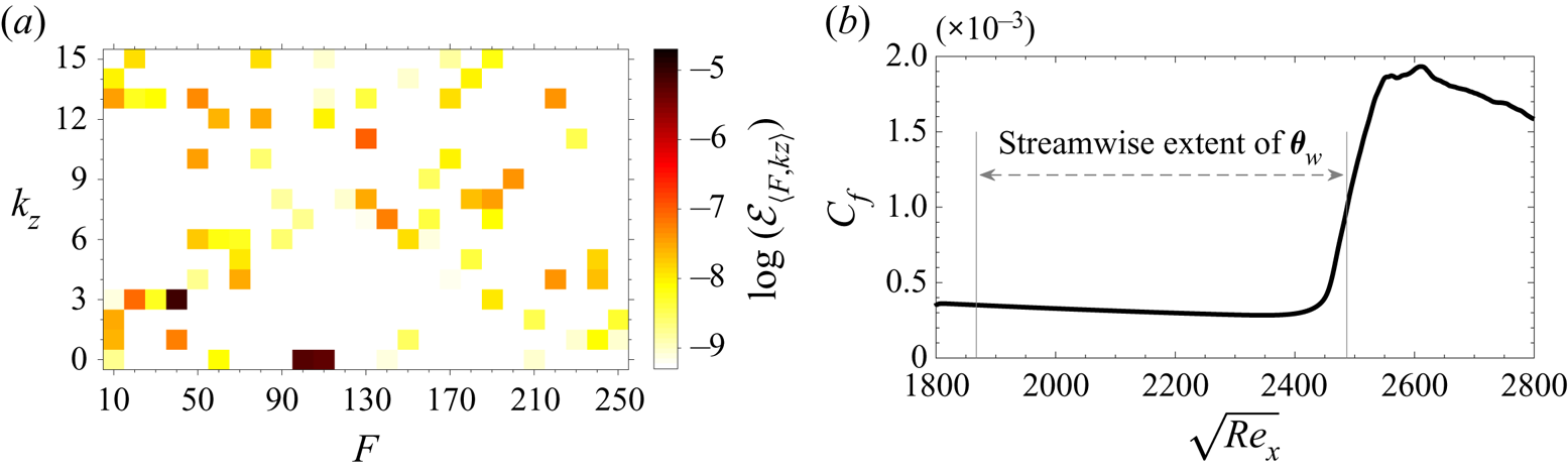
was set to  $\mathcal {E} ( \boldsymbol {\varphi }^{\prime } ) = 2 \times 10^{-5}$. This amount of energy is selected to be relevant to stratospheric flights (Haack, Gerding & Lübken Reference Haack, Gerding and Lübken2014). The spectral makeup of the inflow disturbance is that of the nonlinearly most dangerous disturbance that causes the earliest upstream transition location over an adiabatic wall, and is shown in figure 2(
 $a$) as a function of the normalized frequency,
 \begin{equation} F = \frac{\omega_j}{\sqrt{{Re}_{x_0}}} \times 10^{6} = 10 j \quad \textrm{for} \ j = 1,2,\ldots,25 , \end{equation}
and integer spanwise wavenumber,
 \begin{equation} k_{z} = \frac{\beta_{k} L_z}{2 {\rm \pi}} = k \quad \textrm{for} \ k = 0,1,\ldots,15 , \end{equation}
of the inflow instability waves. The energy spectral density  $\mathcal {E}_{\langle F , k_z \rangle }$ is defined as
 \begin{equation} \mathcal{E}_{\langle F , k_z \rangle } = \tfrac{1}{2} \int_{0}^{L_y} \boldsymbol{\hat{\zeta}}_{\langle F , k_z \rangle }^* \textbf{diag} ( \boldsymbol{\xi} ) \boldsymbol{\hat{\zeta}}_{\langle F , k_z \rangle } \,{\textrm{d} y}, \end{equation}
where  $\boldsymbol {\hat {\zeta }}_{\langle F , k_z \rangle }$ are the two-dimensional Fourier coefficients of the perturbation vector of primitive variables, e.g. at the inlet plane
 $\boldsymbol {\hat {\zeta }}_{\langle F , k_z \rangle } \equiv \boldsymbol {\hat {\varphi }}_{\langle F , k_z \rangle }$, the star symbol denotes the complex conjugate transpose, and the term
 $\boldsymbol {\xi } = [ ({R}/({\gamma -1}))({\bar {T}}/{ \bar {\rho }}) \ \bar {\rho } \ \bar {\rho } \ \bar {\rho } \ ({R}/({\gamma -1})) ({\bar {\rho }}/{\bar {T}}) ]^{tr}$ ensures that the kinetic and internal energy are appropriately weighted.
 $(a)$ The energy content of the instability waves at the inlet plane and
 $(b)$ the corresponding streamwise change of skin-friction coefficient along an adiabatic wall. For the definitions of
 $F$,
 $k_z$ and
 $\mathcal {E}$ see (3.3) to (3.5), whereas
 $\boldsymbol {\theta }_w$ is computed from (2.5).

Figure 2( $a$) shows that most of the total energy, approximately 95 %, is allocated in only three inlet waves:
 $\langle 40 , 3 \rangle$,
 $\langle 100 , 0 \rangle$ and
 $\langle 110 , 0 \rangle$. In the established terminology of linear stability theory, at the inlet location of the current simulations
 $\langle 100 , 0 \rangle$ and
 $\langle 110 , 0 \rangle$ are second-mode instabilities while
 $\langle 40 , 3 \rangle$ is a first-mode wave. The procedure that was adopted to determine this nonlinearly most dangerous disturbance, and a detailed discussion for its makeup and transition mechanism were presented by Jahanbakhshi & Zaki (Reference Jahanbakhshi and Zaki2019).
The final boundary is the wall, where all velocity components satisfy the no-slip condition. The normal heat flux is computed using the parameterization (2.5) and is explicitly imposed in the energy equation as part of the viscous flux. In order to enable localized cooling and heating in our analysis, the streamwise parameterization of the heat flux vector is performed in terms of Gaussian functions, with centres located at  $x_n = x_1 + (n-1) {\rm \Delta} L$ and standard deviations
 $\sigma = w_g {\rm \Delta} L$. The centre of the first and last Gaussians are located at the streamwise positions
 $x_1 = 1937$ and
 $x_2 = 3436$, consecutive Gaussians are separated by
 ${\rm \Delta} L = (x_2 - x_1)/(M_x-1)$, and
 $w_g = 0.8085$ is a precomputed parameter that determines the width of the Gaussian functions such that they provide the best parameterization of the wall heat flux; the details of how
 $w_g$ is computed are provided in Appendix A. The Gaussians are then orthonormalized and, in that form, are denoted
 $\boldsymbol {g}_n$ in (2.5).
The inflow condition for the current simulations is the nonlinearly most dangerous disturbance for an adiabatic wall, and therefore the wall heat flux intended to delay transition starts at  $x_1 > x_0$. Furthermore, the location of the centre of the last Gaussian,
 $x_2$, is chosen to ensure that heat flux is not applied to the turbulent region: a hot wall would increase the viscosity of the gas which would result in a thicker boundary layer and a reduced skin friction inside the turbulent zone. As such, a possible outcome of an optimization algorithm that aims to minimize the skin friction is a very hot wall that suppresses the contribution to the cost function in the turbulent region, instead of delaying transition. In order to ensure that the EnVar optimization focuses on the true objective of delaying transition, the downstream extent over which the optimization of the heat flux is performed is restricted to
 $x_2$. Figure 2(
 $b$) depicts the skin-friction coefficient corresponding to marching the inlet disturbance when the plate is adiabatic, and the streamwise extent (
 $x_1 < x < x_2$) where the wall heat flux will be applied in our analysis, is identified.
We verified that our prediction of transition is grid independent. The resolution also ensured that we resolve the instability modes prescribed at the inlet and their nonlinear interaction, leading to transition. For the instability modes that play a significant role in the progression of transition to turbulence, the grid comprises a minimum of 20 points per streamwise wavelength and a minimum of 36 points per spanwise wavelength. In the wall-normal direction, a minimum of 40 points are inside the boundary layer.
4. Results and discussions
4.1. Optimal surface heat flux
The cost function of the optimization is  $\mathcal {J} \equiv \frac {1}{2} \Vert \mathcal {G} ( \textbf {q} ) \Vert ^2 = ({1}/{2 L_x}) \int _{x_0}^{x_f} C_f^2 \,{\textrm {d} x}$ where
 $C_f$ is the skin friction coefficient. This cost function targets an observable that is a nonlinear function of the inflow disturbance and also of the control vector. As such, the optimization does not attempt to stabilize any particular instability mode because such action can destabilize another; the optimization targets delaying transition which is only assured by disrupting antecedent nonlinear interactions without generating new more aggressive ones (see § 4.2). Any approach based on linear theory cannot make such a guarantee.
In order to demonstrate that the outcome of minimizing  $\mathcal {J}$ is transition delay,
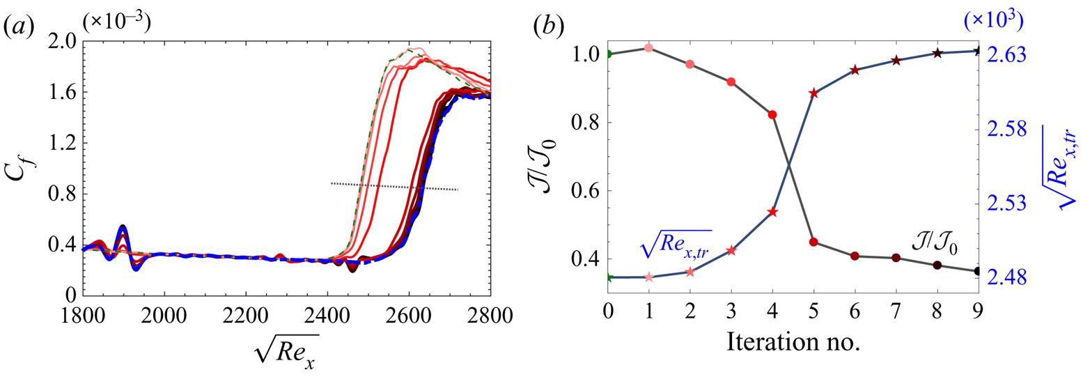
 $C_f$ curves for consecutive iterations of the EnVar algorithm are reported in figure 3. The results demonstrate that the optimal heat flux indeed shifts the transition location downstream, and also leads to oscillations in the laminar skin friction relative to the Blasius solution. For this reason, conventional definitions of the transition Reynolds number, e.g. minimum
 $C_f$, are not applicable. Instead, we defined the transition Reynolds numbers in panel (b) as the location where the skin friction reaches
 $\frac {1}{2}( C_{f,lam} + C_{f,turb} )$, where
 $C_{f,lam}$ and
 $C_{f,turb}$ are the laminar value and turbulent correlation for Mach 4.5 over an adiabatic flat plate (equations (7-39) and (7-132) in White (Reference White2006)). The same panel also reports the cost function normalized by its initial value from the reference adiabatic flow. After the seventh iteration, the delay in transition location and the change in the cost function become marginal, which is a sign of convergence. In addition to these trends, another important stopping criterion of the optimization algorithm is the minimum instantaneous wall temperature, which we restricted to
 $T_{wall} / T_\infty > 0.4$ for practical considerations. This criterion was reached at the ninth iteration, and continuing the optimization procedure results in even smaller temperatures at the wall. While an instantaneous wall temperature
 $T_{wall} / T_\infty \approx 0.4$ (
 $T_{wall} / T_{ad} \approx 0.1$) is small, it is not unlike values reported in laboratory experiments (see e.g. Sanator, DeCarlo & Torrillo Reference Sanator, DeCarlo and Torrillo1965; Wallace Reference Wallace1967; Chien Reference Chien1973). In terms of the commonly reported ratio of the mean wall-temperature to the adiabatic value, at the final iteration this quantity has the range
 $0.37 \leq \bar {T}_{wall} / T_{ad} \leq 1.12$, which is comparable to previous studies (Lysenko & Maslov Reference Lysenko and Maslov1984; Fedorov et al. Reference Fedorov, Soudakov, Egorov, Sidorenko, Gromyko, Bountin, Polivanov and Maslov2015; Bountin et al. Reference Bountin, Maslov and Gromyko2018). Another notable observation from figure 3(
 $a$) is that the optimal wall heat flux eliminates the skin-friction overshoot beyond the turbulent curve that typically takes place at the end of the transition zone (Franko & Lele Reference Franko and Lele2013; Marxen & Zaki Reference Marxen and Zaki2019).
 $(a)$ Skin friction and
 $(b)$ normalized cost function and transition Reynolds number. In the
 $C_f$ plots, the dashed green profile correspond to the initial guess, and thin to thick (also light- to dark-coloured) solid lines represent the result for the mean control vector after consecutive iterations of EnVar algorithm, the dashed-dotted blue curves correspond to the DNS of the reduced heat flux vector depicted in figure 4(
 $c$), and the dotted black line is the average of the theoretical skin friction of laminar and turbulent regions.

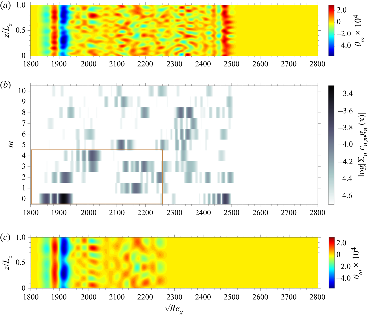
The optimal heat flux after the final iteration is reported in figure 4(a,b). Panel (a) shows the heat flux in two-dimensional physical space, and highlights the localized nature of the heating and cooling. In particular, the region  $\sqrt {Re_x} < 2000$ appears to be most influential: it is the site of the maximum heat flux which is applied in three consecutive, nearly two-dimensional strips of cooling, heating and subsequent cooling. Figure 4(
 $b$) shows the same result but with the spanwise direction shown in wavenumber space, and the contours corresponds to the heat flux spectral density,
 $| \sum _{n = 1}^{ M_x } c_{n,m} \boldsymbol {g}_n |$, as a function of streamwise location – see (2.5). The results identify
 $m = 0$ and
 $2$ as the most important integer wavenumbers in the upstream zone; that region is also host to the synchronization points of the two inlet two-dimensional waves that have most of the energy, i.e. instability waves
 $\langle 110 , 0 \rangle$ and
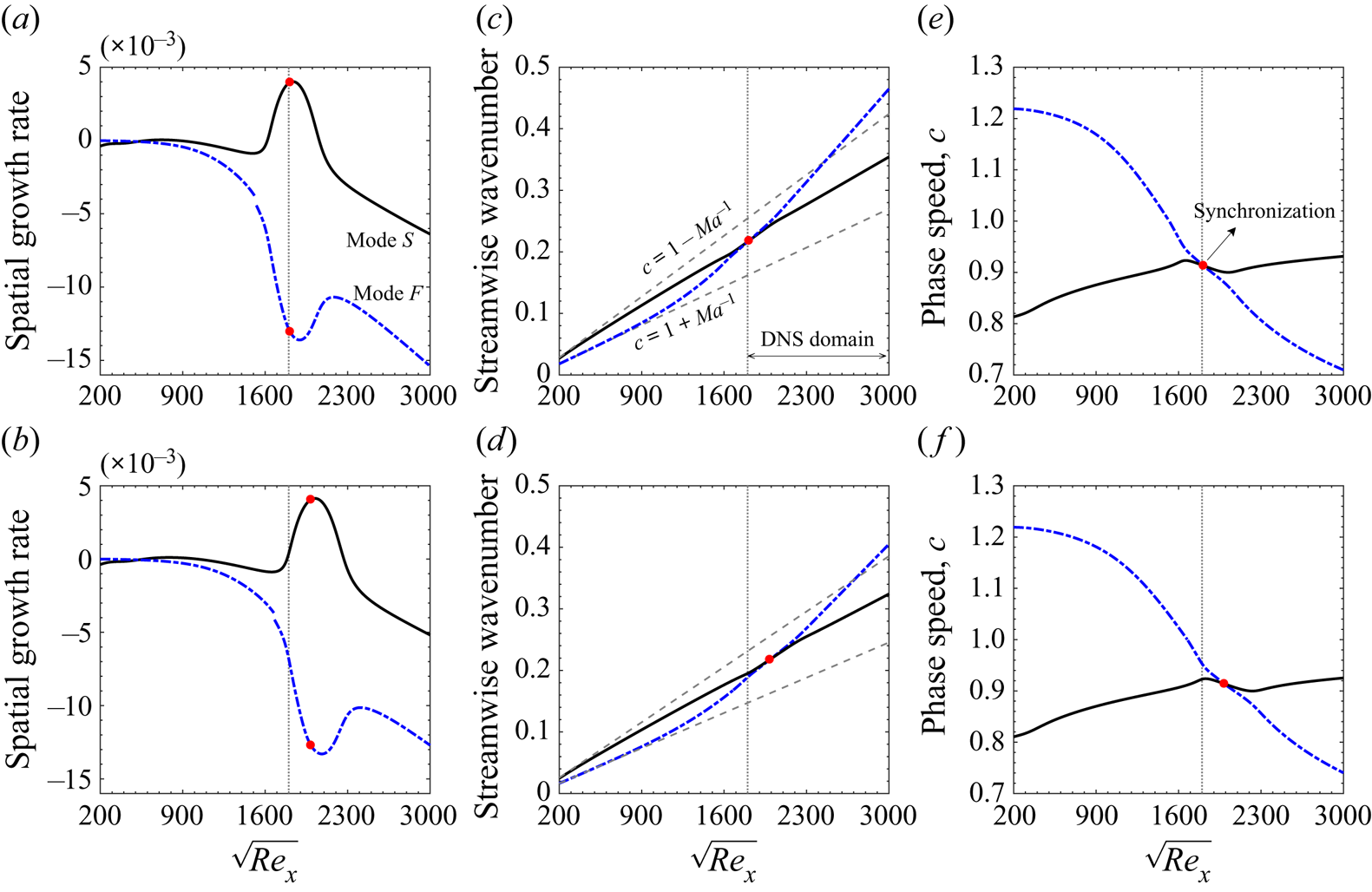
 $\langle 100 , 0 \rangle$ in figure 2. The spatial growth rates, streamwise wavenumbers and phase speeds of modes
 $F$ and
 $S$ at those frequencies are plotted as a function of Reynolds number in figure 5. The figure is evaluated using parallel linear theory, and shows the typical characteristics of slow and fast modes (Fedorov Reference Fedorov2011; Fedorov & Tumin Reference Fedorov and Tumin2011; Park & Zaki Reference Park and Zaki2019): (i) at low Reynolds number modes
 $S$ and
 $F$ appear, respectively, near the slow acoustic,
 $c = 1 - 1/Ma _{\infty }$, and fast acoustic,
 $c = 1 + 1/Ma _{\infty }$, branches of the spectrum; (ii) the former accelerates and the later decelerates with Reynolds number until they synchronize; and (iii) the profiles of mode
 $F$ show a discontinuity at the location where its phase speed approaches
 $c = 1$ from either side which corresponds to crossing the continuous branch of entropy and vorticity modes. The synchronization Reynolds numbers for
 $\langle F , k_z \rangle = \langle 100 , 0 \rangle$ is at
 $\sqrt {Re_x} = 1988$ and for
 $\langle F , k_z \rangle = \langle 110 , 0 \rangle$ it is
 $\sqrt {Re_x} = 1811$. The latter is close to the inlet, and upstream of the region where heating/cooling is applied. In contrast, the synchronization point of the lower frequency mode
 $\langle F , k_z \rangle = \langle 100 , 0 \rangle$ is within the control region. Note that the peak of the first Gaussian distributions used to parameterize the heat flux vector is at
 $\sqrt {Re_{x_1}} \approx 1867$; that of the seventh Gaussian is located at
 $\sqrt {Re_x} \approx 1988$, exactly at the synchronization point of that mode. The presynchronization zone of mode
 $\langle 100 , 0 \rangle$ is thus more aggressively targeted by the optimal thermal texture (cf. figure 4), although its postsynchronization flow is also within the heat flux zone. These observations are consistent with the notion that the synchronization point of instability waves is a key modulator of stability in thermally treated boundary layers (Zhao et al. Reference Zhao, Wen, Tian, Long and Yuan2018; Park & Zaki Reference Park and Zaki2019).
 $(a)$ Surface heat flux of the optimized solution after the final iteration in physical space,
 $(b)$ amplitudes of heat flux complex coefficients of the optimized solution in spectral space and
 $(c)$ surface heat flux of the reduced heat flux case in physical space. The marked rectangular region in panel
 $(b)$ represents the streamwise extent and the range of spanwise wavenumber of the reduced heat flux vector.

(a,b) Spatial growth rate, (c,d), streamwise wavenumber and (e,f) phase speed, of modes S (solid line) and F (dashed-dotted lines) corresponding to the instabilities  $\langle 110 , 0 \rangle$, (a,c,e) and
 $\langle 100 , 0 \rangle$, (b,d,f). The red dots indicate the synchronization point, the dotted lines mark the start of the computational domain in our DNS, and the dashed lines represent the phase speed of acoustic waves.

In order to further isolate the most important spanwise wavenumbers and streamwise extent of the surface heat flux that are responsible for the delay of transition, several test cases with a reduced heat flux vector compared with the optimized solution were examined. Using representation (2.5) of the optimal heat flux and only retaining  $M_z = 4$ and
 $M_x = 21$ (relative to the full range
 $M_z = 10$ and
 $M_x = 36$), the transition delay as indicated by the skin friction curve is similar to that of the optimal solution. This reduced heat flux vector in spectral and physical spaces is shown in figures 4(
 $b$) and 4(
 $c$), respectively, and the corresponding
 $C_f$ curve is reported in figure 3(
 $a$) (blue dashed-dotted line). The power expended for heating and cooling the plate in this case was
 $\int _z \int _x | \boldsymbol {\theta }_w | \,\textrm {d} x\, \textrm {d} z \approx 11$ non-dimensional units. Hereafter, the focus will be placed on this reduced form of the optimal wall heat flux.
4.2. Transition mechanism
Here we compare the mechanisms by which the boundary layer transitions to turbulence in two DNS: the first corresponds to the reference simulation, or the evolution of the inflow condition shown in figure 2 over an adiabatic flat plate; in the second DNS, the optimal heat flux from figure 4( $c$) is applied. All other physical and numerical parameters of these two calculations are identical as provided in table 2. These two cases will hereafter be referred to as NAd and NHF, respectively, where the letter ‘N’ refers to the nonlinearly most-dangerous inflow disturbance and the two subsequent letters designate the wall thermal condition (adiabatic (Ad); heat flux(HF)).
Physical and computational parameters for the simulations designed to examine effects of thermal-roughness on the transition mechanism.

Figure 6 is a visualization of some of the flow structures using isosurfaces of the second invariant of the velocity gradient tensor. In both cases, turbulence is initiated via the formation and breakdown of  $\varLambda$-shaped vortices. As captured qualitatively in this figure, once hairpin vortices are formed, small-scale structures are generated immediately downstream and breakdown to a fully turbulent state takes place over a short streamwise extent. The primary impact of the surface hear flux is (i) attenuation of some of the two-dimensional structures near the wall; (ii) stalling of the formation of three-dimensional
 $\varLambda$-shaped vortices which results in a delayed transition to turbulence; and (iii) a far less-aggressive generation of small-scale turbulent structures along the nonlinear transitional zone, which is consistence with the disappearance of the skin-friction overshoot reported in connection with figure 3(
 $a$). Figure 6 also reveals that although most of the heat flux is applied in the upstream low-Reynolds-number region (
 $\sqrt {Re_x} < 1950$), the delayed response to the thermal treatment becomes visible farther downstream (
 $\sqrt {Re_x} > 2250$) and is carried over into the turbulent zone.
Flow structures visualized by  $Q = 1 \times 10^{-4}$ isosurfaces corresponding to cases
 $(a)$ NAd and
 $(b)$ NHF. The contour colours correspond to heat flux,
 $\boldsymbol {\theta }_w$, at the wall, and streamwise velocity perturbation,
 $u^{\prime }$, on the
 $Q$ isosurfaces.

4.2.1. Energy content of the instability waves
An energetic interpretation of the transition process is sought from the streamwise development of the energy spectral density,  $\mathcal {E}_{\langle F , k_z \rangle }$, and the nonlinear energy transfer coefficient among instability waves,
 $\mathcal {I}_{\langle F , k_z \rangle }$. The two quantities are reported in figures 7 and 8. The spectral density
 $\mathcal {E}_{\langle F , k_z \rangle }$ is computed from (3.5), while
 $\mathcal {I}_{\langle F , k_z \rangle }$ is defined as
 \begin{equation} \mathcal{I}_{\langle F , k_{z} \rangle } \equiv \sum_{{\pm} F , \pm k_{z}} \int_{0}^{L_y} \vert \boldsymbol{\hat{\mathcal{A}}}^*_{\langle F_1 , k_{z,1} \rangle } \boldsymbol{\hat{\mathcal{B}}}_{\langle F_2 , k_{z,2} \rangle } + \boldsymbol{\hat{\mathcal{A}}}^*_{\langle -F_2 , -k_{z,2} \rangle } \boldsymbol{\hat{\mathcal{B}}}_{\langle -F_1 , -k_{z,1} \rangle } \vert \,\textrm{d} y . \end{equation}
In (4.1),  $F = F_2 - F_1$,
 $k_z = k_{z,2} - k_{z,1}$, and
 $\boldsymbol {\hat {\mathcal {A}}}$ and
 $\boldsymbol {\hat {\mathcal {B}}}$ are vector quantities containing the Fourier coefficients of
 $\boldsymbol {\mathcal {A}} \equiv [\rho u^{\prime \prime } u^{\prime \prime } \ \rho u^{\prime \prime } v^{\prime \prime } \ \rho u^{\prime \prime } w^{\prime \prime }]^{tr}$ and
 $\boldsymbol {\mathcal {B}} \equiv [ u^{\prime \prime } \ v^{\prime \prime } \ w^{\prime \prime } ]^{tr},$ where the double-primed velocities are the fluctuations with respect to density-weighted mean. The definition of
 $\mathcal {I}_{\langle F , k_z \rangle }$ is obtained from the redistribution term of turbulent kinetic energy by nonlinear interactions of instability waves in the turbulent kinetic energy transport equation (see appendix B of Jahanbakhshi & Zaki (Reference Jahanbakhshi and Zaki2019) for a detailed derivation); it represents the nonlinear energy transfer among the triad
 $\langle F , k_{z} \rangle$,
 $\langle F_1 , k_{z,1} \rangle$ and
 $\langle F_2 , k_{z,2} \rangle$.
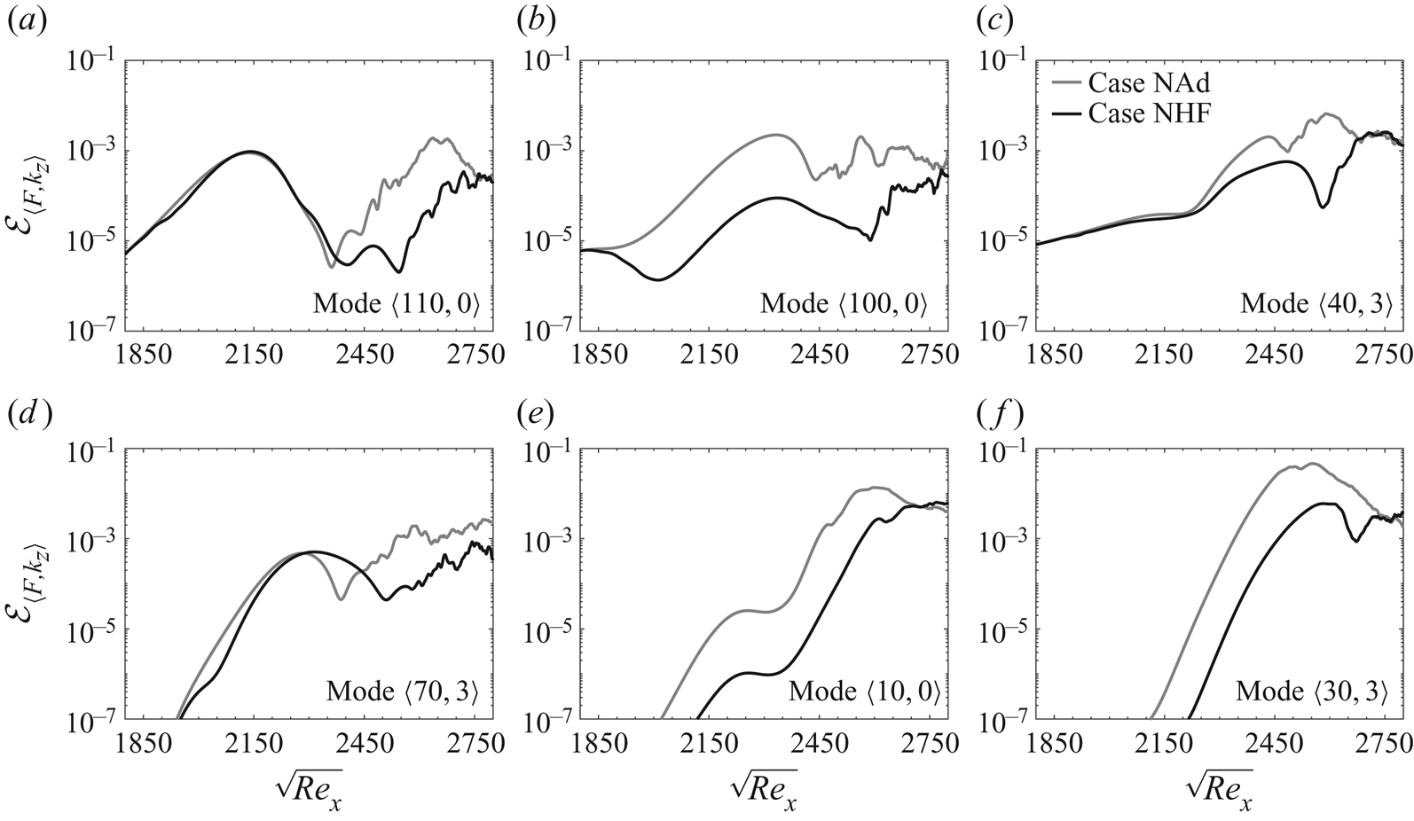
Streamwise development of fluctuations energy content for selected instability modes corresponding to cases NAd (grey lines) and NHF (black lines).

Modal nonlinear energy transfer coefficient for important modal interactions corresponding to cases NAd (grey lines) and NHF (solid lines).

Figures 7 and 8 together provide the following interpretation of the transition scenarios for both NAd and NHF cases; the evolution of the three most energetic inflow instability waves  $\langle 110,0\rangle$,
 $\langle 100,0\rangle$ and
 $\langle 40,3\rangle$ are shown in figure 7(a–c). A series of nonlinear interactions amongst them spur new instabilities, of which the most important ones are
 $\langle 70,3\rangle$,
 $\langle 10,0\rangle$ and
 $\langle 30,3\rangle$ (figure 7d–f). The nonlinearly generated mode
 $\langle 30,3\rangle$ grows faster than any of the instabilities, and contributes to the amplification of streaks
 $\langle F , k_z \rangle = \langle 0 , 6 \rangle$ which are formed by interaction of oblique modes
 $\langle \pm F , 3 \rangle$ (see figure 9 by Jahanbakhshi & Zaki (Reference Jahanbakhshi and Zaki2019)) . Mode
 $\langle 30,3\rangle$ is also part of an important triad interaction with modes
 $\langle 40,3\rangle$ and
 $\langle 10,0\rangle$, which is depicted quantitatively in figure 8(
 $d$). In the late stages just upstream of breakdown to turbulence, that mode leads to the formation of the
 $\varLambda$-shaped vortices observed in the instantaneous fields (cf. figure 6). For a detailed description of the transition scenario, the reader is referred to Jahanbakhshi & Zaki (Reference Jahanbakhshi and Zaki2019).
Comparison of the profiles from cases NAd and NHF indicates that the heat flux primarily attenuates mode  $\langle 100,0\rangle$ and the nonlinear interactions which involve this instability wave (see figures 7b and 8b,c), whereas it has minimal effect on mode
 $\langle 110,0\rangle$. The final, and the most important triad interaction shown in figure 8(
 $d$), is also affected once the flow evolution becomes highly nonlinear, which results in damped amplification of the modes
 $\langle 30,3\rangle$,
 $\langle 40,3\rangle$ and
 $\langle 10,0\rangle$. Combined with the respective locations of the synchronization points of modes
 $\langle 110,0\rangle$ and
 $\langle 100,0\rangle$ (figure 5), the energy spectra indicate that the optimal surface heat flux targets and effectively alters the amplification rate of the latter instability wave whose synchronization point is downstream of the region of pronounced heating/cooling.
An important observation from figure 7( $a$) is the weak influence of heat flux on mode
 $\langle 110,0\rangle$ in the pretransitional region. Zhao et al. (Reference Zhao, Wen, Tian, Long and Yuan2018) have shown recently that in a
 $Ma = 6$ boundary layer, a normal disturbance subjected to cooling downstream of the synchronization point is destabilized while a heating strip is stabilizing; the effects were reversed when the strips were placed upstream of synchronization. The report by Zhao et al. (Reference Zhao, Wen, Tian, Long and Yuan2018) highlights the difficulty of using heating alone or cooling alone to stabilize a flow field that is comprised of multiple unstable modes with different synchronization points, since stabilizing one mode may destabilize another. In our configuration, the optimal heat flux vector from figure 4(
 $c$) is effective at balancing these potentially conflicting effects. The prominent strips of successive cooling, heating and then cooling downstream of the synchronization point of mode
 $\langle 110,0\rangle$ inappreciably alter its evolution, while their placement upstream of the synchronization point of mode
 $\langle 100,0\rangle$ effectively stabilizes that wave. We have verified this interpretation by performing three test simulations where we adopted adiabatic boundary conditions in lieu of (i) the most upstream cooling strip in figure 4(
 $c$) (
 $\sqrt {Re_x} < 1872$); (ii) the most upstream heating strip (
 $1872 < \sqrt {Re_x} < 1896$); and (iii) the first cooling and heating strips (
 $\sqrt {Re_x} < 1896$). The results of these test cases confirmed the above assertion: removing the most upstream cooling and/or heating strip destabilized the flow and moved the transition location upstream when compared with case NHF, and the entire heat flux pattern is indeed required for transition delay. In addition, stabilization of mode
 $\langle 100,0\rangle$ is primarily influenced by the last cooling strip and beyond (
 $\sqrt {Re_x} > 1896$).
A notable difference between the simulations here and the work by Zhao et al. (Reference Zhao, Wen, Tian, Long and Yuan2018) is the characteristic length scale of the thermal strips. For reference, the second-mode instabilities  $\langle 110,0\rangle$ and
 $\langle 100,0\rangle$ have streamwise wavelengths that are approximately
 $2 \delta$, or twice the local boundary layer thickness, in the synchronization region. The length of the heating/cooling strips in the study by Zhao et al. (Reference Zhao, Wen, Tian, Long and Yuan2018) were close to one
 $\delta$ in order to reduce non-parallel effects, and maintain validity of the locally parallel approximation from linear stability theory. In contrast, in the present simulations the width of each of the first two strips is approximately three
 $\delta$ and the third strip is nearly six
 $\delta$. An important modulator of the amplification of the second-mode instabilities is the thickness of the near-wall supersonic region
 $c - u \geq a$, where
 $c$ is the phase speed of the instability and
 $a$ is the local speed of sound. Along this region the pressure waves reflect at the wall and at the relative sonic streamline
 $c - u = a$; at the latter location, the waves change from compression to expansion and vice versa (Morkovin Reference Morkovin1987). These waves are typically phase-tuned with the harmonic vorticity and temperature waves that are travelling along the relative sonic line. For the thin isolated cooling or heating strips adopted by Zhao et al. (Reference Zhao, Wen, Tian, Long and Yuan2018), the thickness of the relative supersonic region changes abruptly thus detuning the waves and altering the growth rate of the second-mode instabilities. In our configuration, the width of the first cooling and heating strips and their relative intensities are such that the thickness of the aforementioned supersonic region is marginally affected (less than 3 %), and there is a minimal change in the growth rate of mode
 $\langle 110,0\rangle$. The third cooling strip, however, shrinks the relative supersonic region more appreciably (approximately 20 %) and stabilizes mode
 $\langle 100,0\rangle$.
4.2.2. Analysis of the FT components of perturbations
Perturbations to high-speed flow prior to interaction with a boundary layer (no mean-shear and/or shock-waves) can be unambiguously described in terms of pressure (acoustic), temperature (entropic) or vorticity (solenoidal) modes. For consistency, we adopt the terminology of Unnikrishnan & Gaitonde (Reference Unnikrishnan and Gaitonde2019) and refer to this classification as the FT components. Presence of a boundary layer, however, obfuscates the interpretation of instability waves in terms of the FT components, even in the linear regime. Nonetheless, such description is desirable because it can provide a physical description of the influence of the thermal texture on transition, and is achieved using momentum potential theory (Doak Reference Doak1989) which identifies the acoustic, entropic (or thermal) and solenoidal (or vortical) components of the momentum density perturbation. This definition of FT components relies on a Helmholtz decomposition which, for a given vector, separates the rotational (solenoidal) component,  $\boldsymbol {S}$, from the irrotational component,
 $\boldsymbol {\nabla } \psi$. The procedure is explained briefly in Appendix B, and for a more detailed description the reader is referred to Doak (Reference Doak1989) and Unnikrishnan & Gaitonde (Reference Unnikrishnan and Gaitonde2019). The wall-normal integrals of the magnitude of the FT components squared,
 $\int _{0}^{L_y} | \bullet |^2 {\textrm {d} y}$, are reported in figures 9 and 10.
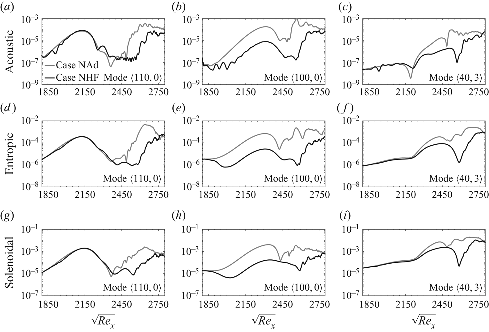
Streamwise development of the square of magnitude of  $(a,b,c)$ acoustic,
 $(d,e,f)$ entropic and
 $(g,h,i)$ solenoidal components of the momentum density associated with the important modes prescribed at the inlet. The profiles are integrated in wall-normal direction.

Streamwise development of the square of magnitude of  $(a,b,c)$ acoustic,
 $(d,e,f)$ entropic and
 $(g,h,i)$ solenoidal components of the momentum density associated with the important nonlinearly generated modes inside the domain. The profiles are integrated in wall-normal direction.

Figure 9 focuses on the instability waves that are present at the inflow and their subsequent evolution inside the computational domain. For the second-mode instabilities,  $\langle 100,0\rangle$ and
 $\langle 110,0\rangle$, the magnitude of the entropic and acoustic components squared are, respectively, one and two orders of magnitude less than the solenoidal component. In contrast, for a first-mode instability, the same two components of the momentum density are significantly smaller. In particular, for mode
 $\langle 40 , 3 \rangle$ the magnitude of the acoustic component squared is approximately three orders of magnitude smaller than the solenoidal one. Comparing the profiles of cases NAd and NHF confirms the effect of heat flux on the pretransitional zone: mode
 $\langle 100 , 0 \rangle$ is the only inflow instability wave that is appreciably affected. All three components of the FT decomposition exhibit a significant drop of energy as heat flux is applied. When the profiles from NHF are normalized by their NAd counterparts (not shown), the acoustic component exhibits the maximum sensitivity and earliest upstream decrease in magnitude. The entropic component is the next to attenuate followed by the solenoidal component. This sequence highlights the physical impact of the thermal texture, which is initially primarily acoustic, followed by the anticipated entropic effect. This observation provides more evidence to support the previous discussion regarding the effect of heat flux on the thickness of the near-wall supersonic region
 $c-u > a$: as this region shrinks, the reflecting acoustic waves become detuned with the harmonic entropic and solenoidal waves which results in stabilization of mode
 $\langle 100 , 0 \rangle$. In figure 10, the FT decomposition is reported for the instability waves that are generated nonlinearly inside the computational domain. The wave
 $\langle 70 , 3 \rangle$ retains the characteristics of a second-mode instability. The other two waves reported in the figure are the outcome of nonlinear interactions involving the inflow mode
 $\langle 100 , 0 \rangle$, and are hence appreciably affected by the thermal wall treatment. They are spurred farther downstream within the computational domain, and become progressively more solenoidal.
It is instructive to evaluate the contribution of each FT component to the energy transfer (see Appendix B). Since the total energy flux has two parts,  $\overline {\rho \boldsymbol {u} h } = \overline {\rho \boldsymbol {u} } \bar { h } + \overline {( \rho \boldsymbol {u} )^{\prime } h^{\prime } }$, we will refer to the fluctuating portion as the mean energy flux due to the momentum fluctuations. Figures 11 and 12 present the contribution of the FT terms to the change of mean energy flux integrated in the wall-normal direction; the former figure is dedicated to instability waves that are prescribed at the inlet and the latter figure to modes that are generated downstream by nonlinear interactions. In order to facilitate comparison of the contributions by the acoustic, entropic and solenoidal components to the mean energy transfer, all ordinates are presented with the same limits.
Streamwise development of the source terms for the change of mean-state due to  $(a,b,c)$ acoustic,
 $(d,e,f)$ entropic and
 $(g,h,i)$ solenoidal components of the important modes prescribed at the inlet. The profiles are integrated in wall-normal direction.

Streamwise development of the source terms for the change of mean-state due to  $(a,b,c)$ acoustic,
 $(d,e,f)$ entropic and
 $(g,h,i)$ solenoidal components of the important nonlinearly generated modes. The profiles are integrated in wall-normal direction.

It is evident from figure 11 that the entropic and acoustic terms, in spite of being relatively small in magnitude (see figure 9), constitute the primary sources of change in mean energy flux due to momentum fluctuations, while the vortical contribution is mostly negative upstream of the turbulent region. The source or sink natures of the FT components are qualitatively similar in the adiabatic and thermally treated cases, although there are significant quantitative differences for some of the modes. The trends are also compatible with earlier observations: the heat flux effectively suppresses all three FT contributions to the mean energy transfer for mode  $\langle 100 , 0 \rangle$ across the entire preturbulent region; for mode
 $\langle 40 , 3 \rangle$, the same effect is observed in the region where triad interactions involving this mode are significant. The impact on these modes should be contrasted to the effect of uniform cooling across the synchronization point that was examined in Mach 6 boundary layer by Unnikrishnan & Gaitonde (Reference Unnikrishnan and Gaitonde2019). They reported a reduction in the magnitude of the vortical and acoustic terms only, while the entropic source which makes the largest contribution to the energy transfer was minimally altered; the authors thus concluded that uniform cooling could potentially destabilize the boundary layer. That study affirms the importance of the streamwise dependence of the optimal texture in order to effectively stabilize the boundary layer.
In figure 12, mode  $\langle 30 , 3 \rangle$ entirely overshadows all the other waves that are generated by the nonlinear interactions. As the trains of hairpin vortices in figure 6 break down to turbulence, all three FT components of the momentum density associated with mode
 $\langle 30 , 3 \rangle$ act as sources that transfer energy from the fluctuation to the mean flow. In particular, the entropic contribution becomes very large relative to the other two contributions. Figure 12 confirms the effectiveness of the thermal texture in stabilizing the boundary layer: the optimal heat flux significantly reduces the transfer of energy to the mean state, even as the flow becomes turbulent which takes place downstream of the thermally treated zone. This observation explains the change in the skin-friction overshoot that is observed during transition in the adiabatic case and is absent in the thermally treated configuration (figure 3
 $a$) – an effect carried over from the upstream thermal treatment. The overwhelmingly large values of entropic and acoustic sources of mean energy flux are mitigated in the controlled flow in the transitional zone and, as a result, the final stages of breakdown to turbulence are not as aggressive as in the adiabatic configuration.
5. Summary and conclusions
A thermal texture is designed to delay transition to turbulence in an originally adiabatic high-speed boundary layer that is exposed to the nonlinearly most dangerous inflow condition. The disturbance is primarily composed of two two-dimensional second-mode instabilities and an oblique first-mode wave, all of which are unstable in the adiabatic configuration. The problem is formulated as a constrained optimization and an EnVar approach is adopted to identify the optimal thermal wall condition that can prolong the laminar region. The algorithm involves an iterative procedure where ensembles of wall heat fluxes are evaluated using DNS, their respective cost functions are computed, and an interior-point method is adopted to update the estimate of the optimal heat flux.
The optimal solution led to a delayed transition to turbulence, and the favourable effect of the surface heat flux persisted farther downstream than the region where it was concentrated. The heat flux effectively subdued a second-mode instability whose fast- and slow-mode synchronization point was downstream of the majority of the applied heat flux. In contrast, the instability characteristics of the second-mode wave with a synchronization point upstream of the thermal texture were minimally affected. As for the first-mode instability, it was only altered in the controlled flow in the nonlinear regime. The optimal heat flux was also able to impede the nonlinear interactions that involved the attenuated instability, and to stall the formation of hairpin vortices that ultimately cause breakdown to turbulence. Observations from the energy spectra are further supported by a detailed analysis of the FT components (acoustic, entropic and solenoidal) of the momentum density vector, and their contributions to the change in the mean energy flux due to momentum fluctuations. The disappearance of the skin-friction overshoot at the onset of the turbulent region and a less aggressive breakdown of hairpin vortices in the thermally treated case are shown to be associated with far less energetic entropic and acoustic contributions to the transfer of energy to the mean flow.
Surface heat flux can stabilize some modes and destabilize others, and can therefore have an unanticipated effect on transition. An important feature of current study is therefore the ability of the optimal thermal texture to definitively delay transition when the inflow condition is comprised of a spectrum of instability waves. In addition, in spite of being restricted to the laminar region of the flow, the effects of the optimal thermal texture extends within the turbulent region and leads to significant reduction of the FT contents of disturbances there and their contribution to the change in the mean energy flux. The results demonstrated the capacity of our optimization strategy to target transition delay, in our configuration and for our flow parameters. The EnVar methodology is, however, general and can be applied to other conditions or configurations of interest. Furthermore, in order to ensure robustness, the design process should include an assessment of performance away from the design condition, for example by examining other environmental disturbances or re-evaluating the nonlinearly most dangerous free stream spectrum for the controlled flow.
Acknowledgements
The authors are grateful to Professor J. Larsson for sharing the Hybrid code.
Funding
The authors acknowledge the financial support from the Office of Naval Research (grant number N00014-17-1-2339) and the US Air Force Office of Scientific Research (grant number FA9550-19-1-0230). Computational resources were provided by the Maryland Advanced Research Computing Center (MARCC).
Declaration of interests
The authors report no conflict of interest.
Appendix A. Streamwise parameterization of heat flux
In the optimization problem, the surface heat flux is the original control vector, which is parameterized using Fourier representation in the spanwise direction and orthonormalized Gaussians in the streamwise direction,
 \begin{equation} \boldsymbol{\theta}_w (x , z) = {\rm Re} \left\{ \sum_{m = 0}^{ M_z } \sum_{n = 1}^{ M_x } c_{n,m} \boldsymbol{g}_n ( x ) \exp \left( \textrm{i} \frac{2 m {\rm \pi}}{L_z} z \right) \right\}. \end{equation}
The original Gaussian distributions  $\boldsymbol {\hat {g}}$ are
 \begin{equation} \boldsymbol{\mathsf{G}} = \begin{bmatrix} \boldsymbol{\hat{g}}_1 & \boldsymbol{\hat{g}}_2 & \ldots & \boldsymbol{\hat{g}}_{M_x} \end{bmatrix} \in \mathbb{R}^{ N_x \times M_x } , \end{equation}
where
 \begin{equation} \boldsymbol{\hat{g}}_n = \exp \left( - \frac{( x - [ x_1 + (n-1) {\rm \Delta} L ] )^2}{2 ( w_g {\rm \Delta} L )^2} \right) .\end{equation}
The parameter  $w_g$ adjusts the width of the Gaussians, and will be optimized such that any location along the streamwise direction is equally well represented by the basis. The orthogonalization is performed using reduced QR factorization of the matrix
 $\boldsymbol{\mathsf{G}}$,
 \begin{equation} \boldsymbol{\mathsf{G}} = \boldsymbol{\mathsf{Q}}_1 \boldsymbol{\mathsf{R}}_1 , \end{equation}
where  $\boldsymbol{\mathsf{Q}}_1 \in \mathbb {R}^{ N_x \times M_x }$ is a matrix that has orthogonal columns and
 $\boldsymbol{\mathsf{R}}_1 \in \mathbb {R}^{ M_x \times M_x }$ is upper triangular. Since the Gaussian functions are linearly independent,
 $\boldsymbol{\mathsf{Q}}_1 = [ \boldsymbol {g}_1 \ \boldsymbol {g}_2 \ \ldots \ \boldsymbol {g}_{M_x} ]$ contains an orthonormal basis for the column space of
 $\boldsymbol{\mathsf{G}}$, or
 $\boldsymbol{\mathsf{Q}}_1^{tr} \boldsymbol{\mathsf{Q}}_1 = \boldsymbol{\mathsf{I}}$. It remains to identify the value of
 $w_g$ in (A2) such that
 $\boldsymbol{\mathsf{Q}}_1$ contains a set of orthonormal basis that can span the control-vector subspace as best as possible, which we achieve using the procedure introduced by Mons et al. (Reference Mons, Wang and Zaki2019).
Any non-zero arbitrary control vector  $\boldsymbol {\chi }$ can be represented using the orthonormalized basis,
 $\boldsymbol {\chi } = \boldsymbol{\mathsf{Q}}_1 \boldsymbol {a}_{\boldsymbol {\chi }}$, where
 $\boldsymbol {a}_{\boldsymbol {\chi }}$ is the weight vector. In other words, the projection of
 $\boldsymbol {\chi }$ onto the subspace spanned by
 $\boldsymbol{\mathsf{Q}}_1$ should be non-zero,
 $\boldsymbol{\mathsf{Q}}_1^{tr} \boldsymbol {\chi } \neq 0$. By satisfying this condition for a certain number of arbitrary control vectors (
 $\boldsymbol {\chi }_{1}$ to
 $\boldsymbol {\chi }_{J}$), the optimum
 $w_g$ can be found by minimizing the cost function,
 \begin{equation} \mathcal{K} = \frac{1}{J} \sum_{j = 1}^{J} \left( \frac{\boldsymbol{\chi}_j^{tr} \boldsymbol{\mathsf{Q}}_1 \boldsymbol{\mathsf{Q}}_1^{tr} \boldsymbol{\chi}_j}{\boldsymbol{\chi}_j^{tr} \boldsymbol{\chi}_j} - \frac{1}{J} \sum_{i=1}^{J} \frac{\boldsymbol{\chi}_i^{tr} \boldsymbol{\mathsf{Q}}_1 \boldsymbol{\mathsf{Q}}_1^{tr} \boldsymbol{\chi}_i}{\boldsymbol{\chi}_i^{tr} \boldsymbol{\chi}_i} \right)^2 .\end{equation}
In the ideal case where  $\boldsymbol{\mathsf{Q}}_1$ represents all of the
 $\boldsymbol {\chi }_{j}$ perfectly,
 $\mathcal {K} = 0$. Any deviation of
 $\mathcal {K}$ from zero is due to the fact that the column space of
 $\boldsymbol{\mathsf{Q}}_1$ cannot be used to span the entire control-vector subspace. Given that in our computations we deal with a discretized domain with
 $\hat {N}_x$ grid points in streamwise direction between
 $x = x_1$ and
 $x = x_2$, we set
 $J = \hat {N}_x$ while
 $\boldsymbol {\chi }_{j}$ is chosen to be integral of Dirac delta functions,
 \begin{equation} \boldsymbol{\chi}_j = \int \delta (x - x_j)\, {\textrm{d} x} = \begin{cases} 1 & \textrm{at} \ x = x_1 + \dfrac{j-1}{J - 1} (x_2 - x_1) \\ 0 & \textrm{elsewhere} \end{cases}\quad \text{for } j=1,2,\ldots J. \end{equation}
The optimization procedure was performed numerically and the optimal  $w_g$ was found to be equal to
 $0.8085$. Figure 13 shows the Gaussian functions corresponding to the optimal
 $w_g$ for a selected number of streamwise indices.
Streamwise parameterization of the surface heat flux:  $(a)$ Gaussian functions and
 $(b)$ orthonormalized Gaussians. Here
 $n$ is the index of each function in streamwise direction, see (2.5).

Appendix B. FT decomposition of perturbations
The momentum density,  $\rho \boldsymbol {u}$, is a vector field which is at least twice continuously differentiable inside the computational domain, and thus Helmholtz's theorem states that it can be decomposed into a curl-free and a divergence-free component,
 \begin{equation} \rho \boldsymbol{u} = \overline{ \rho \boldsymbol{u} } + ( \rho \boldsymbol{u} )^{\prime} = \bar{\boldsymbol{S}} - \boldsymbol{\nabla} \bar{\psi} + \boldsymbol{S}^{\prime} - \boldsymbol{\nabla} \psi^{\prime}, \end{equation}
where
 \begin{equation} \boldsymbol{ \nabla } \boldsymbol{\cdot} \bar{\boldsymbol{S}} = \boldsymbol{ \nabla } \boldsymbol{\cdot} \boldsymbol{S}^{\prime} = 0 . \end{equation}
In a time-stationary flow where  ${ \partial \bar {\bullet }}/{ \partial t} = 0$, the mean scalar-potential
 $\boldsymbol {\nabla } \bar {\psi }$ is both irrotational and solenoidal, and can thus be assumed to be zero without loss of generality. Using the continuity equation,
 $\boldsymbol {\nabla } \boldsymbol {\cdot } (\rho \boldsymbol {u}) = - \partial \rho / \partial t$, and the time-stationary condition, we can evaluate the scalar potential perturbation field,
 \begin{equation} \nabla^2 \psi^{\prime} = \frac{\partial \rho^{\prime} }{\partial t} .\end{equation}
For a gas in equilibrium, one can obtain constitutive trivariate relationships among thermodynamic properties, e.g.  $\rho \equiv \rho ( p , s )$, where
 $s$ is the entropy. Therefore, for an ideal gas, (B3) can be expanded using the equality
 $\delta \rho ^{\prime } = \delta p^{\prime } / a^{2} + ( \partial \rho / \partial s )_p \delta s^{\prime }$, where
 $a = \sqrt { ( \partial p / \partial \rho )_{s} }$ is the speed of sound. As such,
 $\psi ^{\prime }$ can be defined uniquely as the sum of an acoustic (
 $\psi _A^{\prime }$) and an entropic (or thermal,
 $\psi _T^{\prime }$) part,
 \begin{equation} \nabla^2 \psi_A^{\prime} = \frac{1}{a^2} \frac{\partial p^{\prime}}{\partial t} , \quad \nabla^2 \psi_T^{\prime} = \left( \frac{\partial \rho}{ \partial s } \right)_p \frac{\partial s^{\prime}}{\partial t} .\end{equation}
We solve the above Poisson equations in spanwise-wavenumber and frequency space,
 \begin{equation} l^{\prime}(x,y,z,t) = \sum_{j,k} \hat{l}_{j,k}(x,y) \exp [ \textrm{i}( \beta_k z - \omega_j t ) ] ,\end{equation}
where  $l^{\prime }$ denotes a perturbation with respect to the time and spanwise average. Using the above modal representation, in spectral space the gradient operator is defined as
 $\hat { \boldsymbol {\nabla } } \equiv [ ({\partial }/{ \partial x })\ ({\partial }/{ \partial y })\ \textrm {i} \beta _k ]^{tr}$ and the time derivative is
 $({\partial }/{ \partial t }) = - \textrm {i} \omega _j$. By adopting the modal ansatz (B5) in the Poisson (B3), the irrotational component of the disturbances can be obtained via solution of the two-dimensional partial differential equations
 \begin{equation} \frac{ \partial^2 \hat{\psi}_{j,k} }{ \partial x^2 } + \frac{ \partial^2 \hat{\psi}_{j,k} }{ \partial y^2 } - \beta_k^2 \hat{\psi}_{j,k} ={-} \textrm{i} \omega_j \hat{\rho}_{j,k},\end{equation}
and a similar equation can be derived for the acoustic component. Hereafter, we drop the subscripts ( $j,k$) for simplicity, and it is understood that the computations are in spectral space. The equations are then solved numerically in the discretized (
 $x,y$) computational domain to obtain
 $\hat {\psi }_{T} = \hat {\psi } - \hat {\psi }_{A}$ and
 $\hat {\boldsymbol {S}} = \bar {\rho } \hat {\boldsymbol {u}} + \hat {\rho } \bar {\boldsymbol {u}} + \hat { \boldsymbol {\nabla } } \hat {\psi }$. The acoustic, entropic and solenoidal then refer to components of the momentum-density perturbation associated with
 $- \hat { \boldsymbol {\nabla } } \hat {\psi }_A$,
 $- \hat { \boldsymbol {\nabla } } \hat {\psi }_T$ and
 $\hat {\boldsymbol {S} }$, respectively.
In order to evaluate the contribution of each FT component to the energy transfer, starting from the energy and momentum equations for a statistically stationary flow, Doak (Reference Doak1989) showed that the momentum potential theory leads to the following expression for the mean transport of fluctuating total (or stagnation) enthalpy per unit mass,  $h \equiv (E + p)/\rho$, due to the momentum density fluctuations:
 \begin{equation} \boldsymbol{\nabla} \boldsymbol{\cdot} [ \overline{( \rho \boldsymbol{u} )^{\prime} h^{\prime} } ] ={-} \{ \overline{ ( - \boldsymbol{\nabla} \psi^{\prime}_A ) \boldsymbol{\cdot} \boldsymbol{\alpha}^{\prime} } \} - \left\{ \overline{ ( - \boldsymbol{\nabla} \psi^{\prime}_T ) \boldsymbol{\cdot} \boldsymbol{\alpha}^{\prime} - ( \rho T )^{\prime} \frac{\partial s^{\prime} }{ \partial t } } \right\} - \{ \overline{\boldsymbol{S}^{\prime} \boldsymbol{\cdot} \boldsymbol{\alpha}^{\prime} } \}.\end{equation}
Here, the vector  $\boldsymbol {\alpha }^{\prime } = ( \boldsymbol {\varOmega } \times \boldsymbol {u} - T \boldsymbol {\nabla } s - \rho ^{-1} \boldsymbol {\nabla } \boldsymbol {\cdot } \boldsymbol {\tau } )^{\prime }$ is the fluctuating acceleration due to vorticity (Coriolis plus centrifugal), entropy gradient and viscosity (for a detailed derivation, see Doak (Reference Doak1989)). Since the total energy flux has two parts,
 $\overline {\rho \boldsymbol {u} h } = \overline {\rho \boldsymbol {u} } \bar { h } + \overline {( \rho \boldsymbol {u} )^{\prime } h^{\prime } }$, we will refer to the fluctuating portion which is expressed in (B7) as the mean energy flux due to the momentum fluctuations. The source terms on the right-hand side of (B7), in order, define the contribution of acoustic, entropic and solenoidal components of
 $(\rho \boldsymbol {u} )^\prime$ to the change of the mean energy flux. In spectral space, we compute the contribution of each instability wave as
 $( \hat { \boldsymbol {\nabla } } \hat { \psi }_A )^* \hat { \boldsymbol {\alpha } }$,
 $( \hat { \boldsymbol {\nabla } } \hat { \psi }_T )^* \hat { \boldsymbol {\alpha } } - ({ \textrm {i} \omega }/{R}) \hat {p}^* \hat {s}$ and
 $-\hat { \boldsymbol {S} }^* \hat { \boldsymbol {\alpha } }$.