1 Introduction
Superhydrophobic surfaces are formed by decorating a hydrophobic solid substrate with a microstructure of slats or pillars. When the said surface is brought into contact with water, and for sufficiently ‘rough’ underlying texture, air bubbles are trapped in a stable Cassie state within the cavities of the texture. While original interest in superhydrophobic surfaces had to do with their remarkable wetting properties (Quéré Reference Quéré2005, Reference Quéré2008), in the recent decade or so these surfaces have also attracted the attention of fluid mechanists due to their drag-reduction potential (Rothstein Reference Rothstein2010; Bocquet & Lauga Reference Bocquet and Lauga2011).
A canonical problem in this emergent field is that of pressure-driven flow between superhydrophobic surfaces. While the original numerical investigations of such flows made use of molecular-dynamics simulations (Cottin-Bizonne et al. Reference Cottin-Bizonne, Barrat, Bocquet and Charlaix2003, Reference Cottin-Bizonne, Barentin, Charlaix, Bocquet and Barrat2004), most present analyses facilitate continuum descriptions. In particular, Fourier-series expansions, originally used by Lauga & Stone (Reference Lauga and Stone2003) for a circular-tube geometry, have formed the de facto standard method in the analysis of flows about textured surfaces. The application of these expansions to the mixed boundary conditions that naturally appear in the representation of these surfaces readily leads to dual series equations governing the Fourier coefficients; these equations are tantamount to the solution of an infinite algebraic system which is represented by a dense matrix. The application of the Fourier-series methodology to rectangular-channel geometries, characteristic of realistic experiments (Lee, Choi & Kim Reference Lee, Choi and Kim2016), was originally carried out by Sbragaglia & Prosperetti (Reference Sbragaglia and Prosperetti2007); later, Teo & Khoo (Reference Teo and Khoo2009) significantly extended that work. Both Sbragaglia & Prosperetti (Reference Sbragaglia and Prosperetti2007) and Teo & Khoo (Reference Teo and Khoo2009) have assumed zero (or small) protrusion angles of the menisci, thus conveniently dealing with liquid domains of rectangular cross section.
The presence of free surfaces of fixed shape in superhydrophobic systems naturally suggests the possibility of thermocapillary flow activation, a mechanism typically associated with the motion of freely suspended drops and bubbles (Young, Goldstein & Block Reference Young, Goldstein and Block1959; Subramanian Reference Subramanian1981; Subramanian & Balasubramaniam Reference Subramanian and Balasubramaniam2001). An order-of-magnitude estimate for water-based systems (Baier, Steffes & Hardt Reference Baier, Steffes and Hardt2010) reveals that modest temperature gradients of the order of
 $10~\text{K}~\text{cm}^{-1}$
readily lead to significant fluid velocities of several millimetres per second. (Baier et al. (Reference Baier, Steffes and Hardt2010) noted that the Reynolds number in these scenarios is still sufficiently small to warrant the neglect of fluid inertia.) Indeed, the ease by which large thermocapillary velocities are reached at small scales may have considerable effects on pressure-driven superhydrophobic flows under non-isothermal conditions (Hodes et al.
Reference Hodes, Kirk, Karamanis and MacLachlan2017).
The thermocapillary analogue to the problem of pressure-driven flow involves an applied temperature gradient. To the best of my knowledge, there has only been a single theoretical investigation of that problem, namely that of Baier et al. (Reference Baier, Steffes and Hardt2010), who considered liquid flow between two periodically grooved solid surfaces of high thermal conductivity (e.g. silicon). In the longitudinal case, where the temperature gradient is applied along the grooves, the flow component in the groove direction is decoupled from those in the cross-sectional plane. Considering deep channels and making use of the Lorentz reciprocity for Stokes flows (Happel & Brenner Reference Happel and Brenner1965), Baier et al. (Reference Baier, Steffes and Hardt2010) showed that at large distances from the bounding surfaces the longitudinal velocity approaches a far-field uniform value; that value, moreover, is proportional to the slip length pertaining to the comparable shear flow about one of these surfaces.
A fundamental aspect of thermocapillary flows, which is of crucial importance in the above-mentioned problem, has to do with dimensions: since no temperature scale is provided in the problem specification, the imposed temperature-gradient magnitude does not provide any length scale. (The temperature-gradient magnitude provides a stress scale, but the latter cannot be transformed to a characteristic length in the absence of a velocity scale.) The length scale on which spatial variations of the pertinent fields take place must therefore be provided by the problem geometry, namely, the groove-array period (‘pitch’) and the channel depth. This lack of ‘non-geometric’ length scale is pertinent to the deep-channel limit, which may appear to suggest an idealised description in a semi-infinite domain about a single surface. Since the channel depth is lost in such a description, it follows that all pertinent fields must approach a finite limit at distances from the surface that are large compared with the pitch – the only remaining length scale. (This scenario is reminiscent of electro-osmosis, where the applied electric field does not provide a relevant length scale and fluid velocity must therefore approach a finite limit at distances large compared with the Debye width – the electrokinetic analogue of the pitch in the superhydrophobic problem.)
While such a finite limit is indeed attained by the flow components, the idealised semi-bounded idealisation fails when considering the thermal problem. Indeed, the combination of a uniform flow (associated with the above-mentioned limit) and an antiparallel temperature gradient results in an advective accumulation of heat. (It is upon introducing advection where the analogy with electro-osmosis breaks down.) The presumed steady state necessitates a comparable conductive transport of heat towards the surfaces. Such a conductive transport, however, does not take place if the temperature profile is uniform across the channel, thus contradicting the possibility of a ‘far-field’ temperature limit in the cross-sectional plane. Conversely, cross-sectional conduction of heat requires a length scale that is not provided by the semi-bounded geometry. These issues have not been addressed in the longitudinal analysis of Baier et al. (Reference Baier, Steffes and Hardt2010), where the focus was on the longitudinal flow rather than the thermal problem and associated cross-sectional flow. (It is interesting to note that, in their numerical calculations, Baier et al. (Reference Baier, Steffes and Hardt2010) solved the Navier–Stokes equations in a bounded domain. When momentum advection is accounted for, the longitudinal velocity is coupled to the cross-sectional velocity and then also to the thermal problem; in that event, it is impossible to employ a semi-bounded geometry even if interest lies only in the longitudinal flow.)
The preceding comments suggest the desirability of a fresh look at the longitudinal problem considered by Baier et al. (Reference Baier, Steffes and Hardt2010). Our goal is twofold: first, to identify a linkage between the longitudinal velocity and that in the comparable pressure-driven flows, thus generalising the proportionality relation of Baier et al. (Reference Baier, Steffes and Hardt2010) which only applies in the deep-channel limit; and second, to investigate the nonlinearly coupled problem governing the temperature and cross-sectional flow in the latter limit. Of particular interest is the role played by heat advection; indeed, this nonlinear mechanism results in a multitude of unconventional phenomena in the classical problem of thermocapillary drop motion at both small (Zhang, Subramanian & Balasubramaniam Reference Zhang, Subramanian and Balasubramaniam2001) and large (Balasubramaniam & Subramaniam Reference Balasubramaniam and Subramaniam1996; Balasubramaniam & Subramanian Reference Balasubramaniam and Subramanian2000) Marangoni numbers.
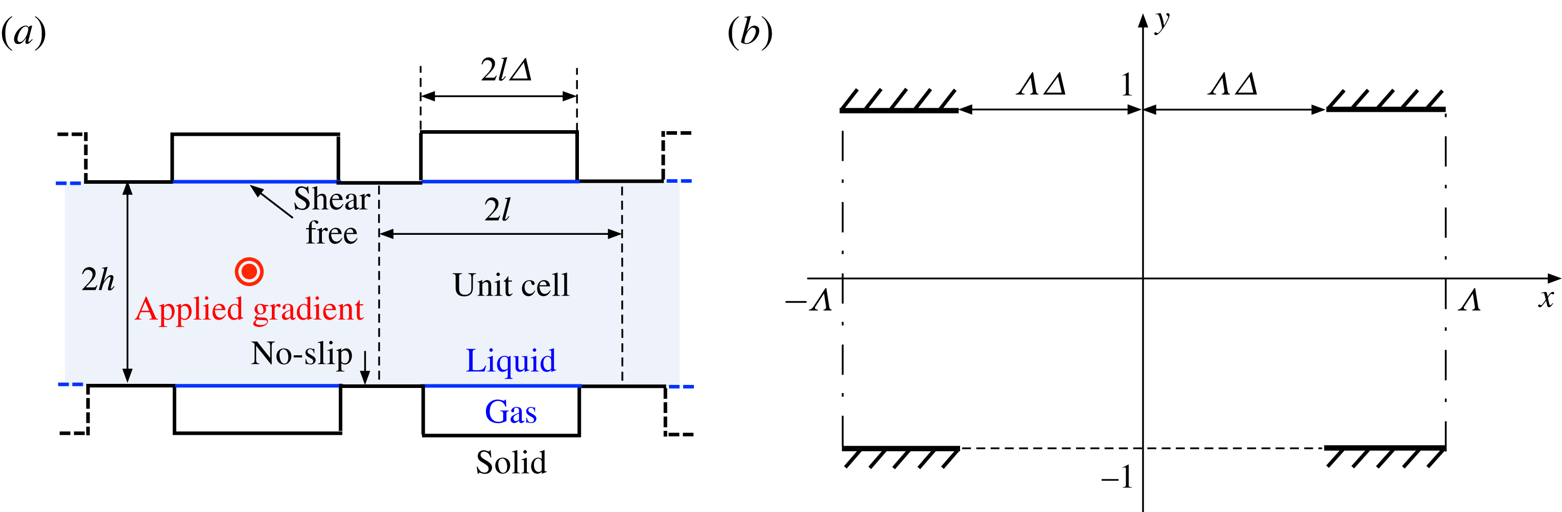
Longitudinal gradient: (a) schematic of the dimensional channel geometry; (b) schematic of the dimensionless unit-cell geometry.

In what follows, we employ the configuration model of Baier et al. (Reference Baier, Steffes and Hardt2010), namely that of a periodic array of highly conducting solid slats separated by flat menisci. Following Baier et al. (Reference Baier, Steffes and Hardt2010) we assume that the thermal diffusivity is constant and employ a linearised dependence of the surface-tension coefficient upon the temperature; these assumptions, which allow for an arbitrary temperature datum, are routinely employed in thermocapillary analyses (Sen & Davis Reference Sen and Davis1982); they are valid provided the typical temperature variations are small. The paper is organised as follows. In § 2 we describe the physical problem and formulate the governing mathematical problem. In § 3 we identify a linkage between the longitudinal flow and that appearing in the comparable problem of pressure-driven flow. The deep-channel limit is introduced in § 4, and the different transport mechanisms that are associated with moderate and large Marangoni numbers are discussed in §§ 5 and 6, respectively. Finally, in § 7 we propose possible future extensions of the longitudinal problem and comment upon the difficulties associated with the comparable transverse problem.
2 Problem formulation
The geometry considered herein is portrayed in figure 1(a). A layer of liquid (viscosity
 $\unicode[STIX]{x1D707}$
, thermal diffusivity
 $\unicode[STIX]{x1D6FC}$
) is confined between two parallel superhydrophobic surfaces, spaced a distance
 $2h$
apart. Each surface is constructed of a periodic array (period
 $2l$
) of flat-edged solid slats. Air is trapped in a stable Cassie state within the grooves bounded by the slats (each groove being of width
 $2l\unicode[STIX]{x1D6E5}$
). The presumably flat liquid–air menisci are pinned at the corners of the slats. The resulting compound surfaces, which bound the liquid domain, are accordingly planar.
We consider the transport processes animated by the application of an external temperature gradient of magnitude
 $G$
parallel to the grooves, assuming that the surface-tension coefficient of the free surface varies linearly with the temperature with a slope
 $\unicode[STIX]{x1D70E}_{T}$
. With the solid material being highly conducting, the temperature distribution therein satisfies a no-flux condition at both the solid–liquid and solid–air interfaces, and is accordingly uncoupled to the temperature profile in the liquid domain. In the present case of longitudinally imposed gradient, the solid-phase temperature distribution is simply provided by a linear variation with the longitudinal coordinate, the slope being
 $G$
. The temperature profile in the liquid, which satisfies a no-flux condition at the free surfaces, must additionally follow (via a Dirichlet condition) that linear variation at the solid–liquid interface.
2.1 Normalisation, coordinates and translational invariance
Using
 $h$
as a length unit, we employ Cartesian coordinates with the
 $z$
-axis antiparallel to the applied-gradient direction, the liquid domain lying between
 $-1<y<1$
, and the plane
 $x=0$
passing through the centres of an opposing pair of menisci (see figure 1
b). Using
 $Gh$
as a temperature unit allows one to define the dimensionless temperature
 $t$
; with the temperature in the present problem being defined to within an arbitrary additive constant, its distribution in the solid substrate is taken simply as
 $t=-z$
. Since the liquid motion is driven by Marangoni stresses at the surfaces, we employ
 $\unicode[STIX]{x1D70F}=-G\unicode[STIX]{x1D70E}_{T}$
as a stress unit (positive in the common case of negative
 $\unicode[STIX]{x1D70E}_{T}$
). With the intrinsic length scale associated with interfacial temperature variations being
 $l$
, it is natural to use
 ${\mathcal{U}}=l\unicode[STIX]{x1D70F}/\unicode[STIX]{x1D707}$
as the velocity unit. The dimensionless problem is governed by two geometric parameters, namely the dimensionless semi-period
 $\unicode[STIX]{x1D6EC}=l/h$
and the gas fraction
 $\unicode[STIX]{x1D6E5}$
. In addition, it depends upon a single dimensionless group, namely the Marangoni number
 $Ma={\mathcal{U}}h/\unicode[STIX]{x1D6FC}$
; upon substituting the derived scale
 ${\mathcal{U}}$
, this number reads
 $$\begin{eqnarray}Ma=\frac{\unicode[STIX]{x1D70F}hl}{\unicode[STIX]{x1D707}\unicode[STIX]{x1D6FC}}.\end{eqnarray}$$
Because of translational invariance in the
 $z$
-direction, the temperature in the liquid domain may be written as
 $$\begin{eqnarray}t=-z+\unicode[STIX]{x1D703},\end{eqnarray}$$
where the excess temperature
 $\unicode[STIX]{x1D703}$
is independent of
 $z$
and is accordingly a function of
 $x$
and
 $y$
alone. Similarly, both the pressure
 $p$
and the velocity components
 $(u,v,w)$
are independent of
 $z$
. (Note that the flow, while being fully developed, is not unidirectional.) Because of the resulting decoupling between the longitudinal flow in the
 $z$
-direction and the flow in the cross-sectional plane, it is convenient to define the cross-sectional velocity vector
 $\boldsymbol{u}=\hat{\boldsymbol{e}}_{x}u+\hat{\boldsymbol{e}}_{y}v$
; the velocity vector is then given as
 $$\begin{eqnarray}\hat{\boldsymbol{e}}_{z}w+\boldsymbol{u}.\end{eqnarray}$$
Given the independence upon
 $z$
, we interpret the gradient operator
 $\unicode[STIX]{x1D735}$
as
 $\hat{\boldsymbol{e}}_{x}\unicode[STIX]{x2202}/\unicode[STIX]{x2202}x+\hat{\boldsymbol{e}}_{y}\unicode[STIX]{x2202}/\unicode[STIX]{x2202}y$
.
Owing to the obvious periodicity, it is sufficient to consider the liquid domain restricted to the ‘unit cell’
 $|x|<\unicode[STIX]{x1D6EC}$
. Given the symmetry about the mid-plane
 $y=0$
, the domain is further restricted to
 $-1<y<0$
.
2.2 The thermal problem
The excess temperature in the ‘semi-cell’ defined above is governed by the energy equation
 $$\begin{eqnarray}\unicode[STIX]{x1D735}\boldsymbol{\cdot }(Ma\,\unicode[STIX]{x1D703}\boldsymbol{u}-\unicode[STIX]{x1D735}\unicode[STIX]{x1D703})=Ma\,w.\end{eqnarray}$$
At
 $y=0$
it satisfies the symmetry condition,
 $$\begin{eqnarray}\frac{\unicode[STIX]{x2202}\unicode[STIX]{x1D703}}{\unicode[STIX]{x2202}y}=0\quad \text{at}~y=0,\end{eqnarray}$$
while at
 $y=-1$
it satisfies a no-flux condition at the free surface,
 $$\begin{eqnarray}\frac{\unicode[STIX]{x2202}\unicode[STIX]{x1D703}}{\unicode[STIX]{x2202}y}=0\quad \text{for}~|x|<\unicode[STIX]{x1D6EC}\unicode[STIX]{x1D6E5},\end{eqnarray}$$
and the temperature-continuity condition at the edges of the solid slats,
 $$\begin{eqnarray}\unicode[STIX]{x1D703}=0\quad \text{for}~\unicode[STIX]{x1D6EC}\unicode[STIX]{x1D6E5}<|x|<\unicode[STIX]{x1D6EC}.\end{eqnarray}$$
In addition, it satisfies the periodicity conditions, which, given the symmetry about
 $x=0$
, simply read
 $$\begin{eqnarray}\frac{\unicode[STIX]{x2202}\unicode[STIX]{x1D703}}{\unicode[STIX]{x2202}x}=0\quad \text{at}~x=\pm \unicode[STIX]{x1D6EC}.\end{eqnarray}$$
2.3 Longitudinal and cross-sectional flow
Neglecting fluid inertia, the flow problem nicely decouples into two subproblems, which respectively govern the longitudinal and cross-sectional flows. The longitudinal velocity component
 $w$
is governed by Laplace’s equation,
 $$\begin{eqnarray}\unicode[STIX]{x1D6FB}^{2}w=0,\end{eqnarray}$$
representing the absence of a macroscopic pressure gradient. At the centreline of the cell, it satisfies a symmetry condition,
 $$\begin{eqnarray}\frac{\unicode[STIX]{x2202}w}{\unicode[STIX]{x2202}y}=0\quad \text{at}~y=0.\end{eqnarray}$$
At
 $y=-1$
it satisfies a Marangoni condition at the free surface,
 $$\begin{eqnarray}\frac{\unicode[STIX]{x2202}w}{\unicode[STIX]{x2202}y}=-\unicode[STIX]{x1D6EC}^{-1}\quad \text{for}~|x|<\unicode[STIX]{x1D6EC}\unicode[STIX]{x1D6E5},\end{eqnarray}$$
and a no-slip condition at the edges of the solid slats,
 $$\begin{eqnarray}w=0\quad \text{for}~\unicode[STIX]{x1D6EC}\unicode[STIX]{x1D6E5}<|x|<\unicode[STIX]{x1D6EC}.\end{eqnarray}$$
Finally, it satisfies the periodicity conditions,
 $$\begin{eqnarray}\frac{\unicode[STIX]{x2202}w}{\unicode[STIX]{x2202}x}=0\quad \text{at}~x=\pm \unicode[STIX]{x1D6EC}.\end{eqnarray}$$
Note that, beyond being uncoupled to the cross-sectional flow, the longitudinal velocity is independent of the excess temperature, and hence of the Marangoni number.
The cross-sectional flow is governed by the continuity equation,
 $$\begin{eqnarray}\unicode[STIX]{x1D735}\boldsymbol{\cdot }\boldsymbol{u}=0,\end{eqnarray}$$
and the Stokes equation, which implies that the vorticity (whose only non-zero component is in the
 $z$
-direction) is harmonic,
 $$\begin{eqnarray}\unicode[STIX]{x1D6FB}^{2}\left(\frac{\unicode[STIX]{x2202}v}{\unicode[STIX]{x2202}x}-\frac{\unicode[STIX]{x2202}u}{\unicode[STIX]{x2202}y}\right)=0.\end{eqnarray}$$
At
 $y=0$
the following symmetry conditions apply,
 $$\begin{eqnarray}v=\frac{\unicode[STIX]{x2202}u}{\unicode[STIX]{x2202}y}=0\quad \text{at}~y=0.\end{eqnarray}$$
At
 $y=-1$
the flow satisfies impermeability,
 $$\begin{eqnarray}v=0,\end{eqnarray}$$
as well as the Marangoni condition at the free surface,
 $$\begin{eqnarray}\frac{\unicode[STIX]{x2202}u}{\unicode[STIX]{x2202}y}=\unicode[STIX]{x1D6EC}^{-1}\frac{\unicode[STIX]{x2202}\unicode[STIX]{x1D703}}{\unicode[STIX]{x2202}x}\quad \text{for}~|x|<\unicode[STIX]{x1D6EC}\unicode[STIX]{x1D6E5},\end{eqnarray}$$
and the no-slip condition at the solid slats,
 $$\begin{eqnarray}u=0\quad \text{for}~\unicode[STIX]{x1D6EC}\unicode[STIX]{x1D6E5}<|x|<\unicode[STIX]{x1D6EC}.\end{eqnarray}$$
Last, the periodicity conditions read
 $$\begin{eqnarray}u=\frac{\unicode[STIX]{x2202}v}{\unicode[STIX]{x2202}x}=0\quad \text{at}~x=\pm \unicode[STIX]{x1D6EC}.\end{eqnarray}$$
2.4 General observations
Three observations readily follow. First, we note that the excess temperature and cross-sectional flow are mutually and nonlinearly coupled through both the Marangoni condition (2.18) and the energy equation (2.4). Upon substitution of the continuity equation (2.14), the latter adopts the more convenient advection–diffusion form,
 $$\begin{eqnarray}Ma(\boldsymbol{u}\boldsymbol{\cdot }\unicode[STIX]{x1D735}\unicode[STIX]{x1D703}-w)=\unicode[STIX]{x1D6FB}^{2}\unicode[STIX]{x1D703}.\end{eqnarray}$$
The longitudinal problem, however, is neither affected by nor affects the thermal problem.
Second, the nonlinear problem formulated above possesses obvious symmetries. We have already exploited the symmetry about
 $y=0$
. In addition, it is readily observed that
 $\unicode[STIX]{x1D703}$
,
 $w$
and
 $v$
are even functions of
 $x$
, while
 $u$
is an odd function of it.
Third, we notice that the only inhomogeneity in the thermal problem enters through the energy equation (2.4). When
 $Ma=0$
that equation becomes homogeneous, and the solution of the thermal problem is the trivial one,
 $\unicode[STIX]{x1D703}\equiv 0$
. Since the only inhomogeneity in the cross-sectional flow problem enters through the Marangoni condition (2.18), it then follows that this problem also possesses the trivial solution,
 $\boldsymbol{u}\equiv \mathbf{0}$
.
2.5 Streamfunction formulation
With the pressure playing only a passive role in the cross-sectional flow problem, it is convenient to employ the streamfunction
 $\unicode[STIX]{x1D713}$
, defined by
 $$\begin{eqnarray}u=\frac{\unicode[STIX]{x2202}\unicode[STIX]{x1D713}}{\unicode[STIX]{x2202}y},\quad v=-\frac{\unicode[STIX]{x2202}\unicode[STIX]{x1D713}}{\unicode[STIX]{x2202}x}.\end{eqnarray}$$
(Since
 $\unicode[STIX]{x1D713}$
is defined to within an arbitrary additive constant, it may be assumed – with no loss of generality – to be odd in
 $x$
.) This function is biharmonic (cf. (2.15)),
 $$\begin{eqnarray}\unicode[STIX]{x1D6FB}^{4}\unicode[STIX]{x1D713}=0,\end{eqnarray}$$
and possesses a nil uniform value at the boundary of the semi-cell,
 $$\begin{eqnarray}\unicode[STIX]{x1D713}=0\quad \text{on both}~y=-1,0~\text{and}~x=\pm \unicode[STIX]{x1D6EC}.\end{eqnarray}$$
In addition, it satisfies the symmetry condition at the cell centreline,
 $$\begin{eqnarray}\frac{\unicode[STIX]{x2202}^{2}\unicode[STIX]{x1D713}}{\unicode[STIX]{x2202}y^{2}}=0\quad \text{at}~y=0,\end{eqnarray}$$
the mixed conditions at the compound surface
 $y=-1$
,
 $$\begin{eqnarray}\frac{\unicode[STIX]{x2202}^{2}\unicode[STIX]{x1D713}}{\unicode[STIX]{x2202}y^{2}}=\unicode[STIX]{x1D6EC}^{-1}\frac{\unicode[STIX]{x2202}\unicode[STIX]{x1D703}}{\unicode[STIX]{x2202}x}\quad \text{for}~|x|<\unicode[STIX]{x1D6EC}\unicode[STIX]{x1D6E5},\quad \frac{\unicode[STIX]{x2202}\unicode[STIX]{x1D713}}{\unicode[STIX]{x2202}y}=0\quad \text{for}~\unicode[STIX]{x1D6EC}\unicode[STIX]{x1D6E5}<|x|<\unicode[STIX]{x1D6EC},\end{eqnarray}$$
and the periodicity conditions
 $$\begin{eqnarray}\frac{\unicode[STIX]{x2202}^{2}\unicode[STIX]{x1D713}}{\unicode[STIX]{x2202}x^{2}}=0\quad \text{at}~x=\pm \unicode[STIX]{x1D6EC}.\end{eqnarray}$$
3 Longitudinal velocity: linkage to pressure-driven flows
Practical interest typically lies not in the detailed solution but rather in the mean longitudinal velocity
 $\langle w\rangle$
, which provides a measure of the superhydrophobic ‘effectiveness’ (Lauga & Stone Reference Lauga and Stone2003). Here, the averaging operator is defined as
 $$\begin{eqnarray}\langle \cdots \rangle =\frac{1}{2\unicode[STIX]{x1D6EC}}\int _{-\unicode[STIX]{x1D6EC}}^{\unicode[STIX]{x1D6EC}}\,\text{d}x\int _{-1}^{0}\,\text{d}y\,\cdots \,.\end{eqnarray}$$
Towards calculation of
 $\langle w\rangle$
, we note a linkage between the problem governing
 $w$
and the comparable superhydrophobic problem governing pressure-driven flows. Thus, defining
 $$\begin{eqnarray}\grave{w} =w+\frac{1-y^{2}}{2\unicode[STIX]{x1D6EC}},\end{eqnarray}$$
we find that
 $\grave{w}$
satisfies the Poisson equation,
 $$\begin{eqnarray}\unicode[STIX]{x1D6FB}^{2}\grave{w} =-\unicode[STIX]{x1D6EC}^{-1},\end{eqnarray}$$
together with a set of homogenous conditions, consisting of the symmetry condition at
 $y=0$
,
 $\unicode[STIX]{x2202}\grave{w} /\unicode[STIX]{x2202}y=0$
, the mixed conditions at
 $y=-1$
,
 $$\begin{eqnarray}\frac{\unicode[STIX]{x2202}\grave{w} }{\unicode[STIX]{x2202}y}=0\quad \text{for}~|x|<\unicode[STIX]{x1D6EC}\unicode[STIX]{x1D6E5},\quad \grave{w} =0\quad \text{for}~\unicode[STIX]{x1D6EC}\unicode[STIX]{x1D6E5}<|x|<\unicode[STIX]{x1D6EC},\end{eqnarray}$$
and periodicity at
 $x=\pm \unicode[STIX]{x1D6EC}$
, where
 $\unicode[STIX]{x2202}\grave{w} /\unicode[STIX]{x2202}x=0$
. In terms of this reduced field, the mean velocity
 $\langle w\rangle$
is given by
 $$\begin{eqnarray}\langle w\rangle =\langle \grave{w} \rangle -\frac{1}{3\unicode[STIX]{x1D6EC}}.\end{eqnarray}$$
The problem satisfied by
 $\grave{w}$
is the same as that governing the flow due to a longitudinal pressure gradient of (dimensionless) magnitude
 $\unicode[STIX]{x1D6EC}^{-1}$
that is applied in the negative
 $z$
-direction, for the same channel geometry. The simultaneous appearance of
 $\unicode[STIX]{x1D6EC}$
in both the differential equation and the problem geometry is of no significance: the linearity of the problem readily allows one to express
 $\grave{w}$
as the product of
 $\unicode[STIX]{x1D6EC}^{-1}$
with the velocity field which is driven by a unit pressure gradient. The latter problem has been extensively discussed in the literature; in particular, making use of either the Fourier-series solutions of Teo & Khoo (Reference Teo and Khoo2009) or the exact solution of Marshall (Reference Marshall2017) one may readily provide
 $\langle \grave{w} \rangle$
for arbitrary numerical values of
 $\unicode[STIX]{x1D6EC}$
and
 $\unicode[STIX]{x1D6E5}$
. Moreover, closed-form approximations for
 $\langle \grave{w} \rangle$
are available in the singular limits of shallow channels (Schnitzer & Yariv Reference Schnitzer and Yariv2017) and small solid fractions (Yariv Reference Yariv2017). Making use of (3.5), these respectively give
 $$\begin{eqnarray}\displaystyle & \displaystyle \langle w\rangle \sim \unicode[STIX]{x1D6EC}\frac{\unicode[STIX]{x1D6E5}^{3}}{3}+\frac{\unicode[STIX]{x1D6E5}^{2}}{\unicode[STIX]{x03C0}}\ln 4+o(1)\quad \text{for}~\unicode[STIX]{x1D6EC}\gg 1, & \displaystyle\end{eqnarray}$$
 $$\begin{eqnarray}\displaystyle & \displaystyle \langle w\rangle \sim \frac{2}{\unicode[STIX]{x03C0}}\ln \frac{1}{1-\unicode[STIX]{x1D6E5}}+O(1)\quad \text{for}~1-\unicode[STIX]{x1D6E5}\ll 1. & \displaystyle\end{eqnarray}$$
4 Deep channels
While the analogy with pressure-driven flows readily provides
 $\langle w\rangle$
via (3.5), it does not shed light on the excess temperature profile and cross-sectional flow structure. In what follows we consider in depth the deep-channel limit,
 $\unicode[STIX]{x1D6EC}\ll 1$
. That limit was (implicitly) considered by Baier et al. (Reference Baier, Steffes and Hardt2010), where the focus was on the longitudinal flow and, in particular, upon the far-field value attained by that flow at large distances away from the boundaries. With that purpose in mind, Baier et al. (Reference Baier, Steffes and Hardt2010) found it convenient to employ an idealised picture involving a semi-bounded fluid domain. As explained in § 1, however, such an idealisation is inconsistent with the energy balance and must therefore be abandoned when considering the coupling between the excess temperature and the cross-sectional flow.
We accordingly employ here inner–outer asymptotic expansions (Hinch Reference Hinch1991), with an inner region of
 $O(\unicode[STIX]{x1D6EC})$
depth adjacent to the boundary
 $y=-1$
and an outer region outside it. (Similar expansions have been used in ‘conventional’ pressure-driven flows between superhydrophobic surfaces; see Kirk, Hodes & Papageorgiou (Reference Kirk, Hodes and Papageorgiou2017).) The inner region is described by the stretched coordinates
 $X$
and
 $Y$
, defined as
 $$\begin{eqnarray}X=\frac{x}{\unicode[STIX]{x1D6EC}},\quad Y=\frac{y+1}{\unicode[STIX]{x1D6EC}}.\end{eqnarray}$$
The outer region, on the other hand, is described by the coordinates
 $X$
and
 $y$
.
4.1 Longitudinal flow
Consider first the longitudinal flow, animated by the Marangoni condition (2.11). This condition, which applies in the inner region, implies that
 $w$
is
 $O(1)$
there. We accordingly employ the asymptotic expansion
 $$\begin{eqnarray}w(x,y;\unicode[STIX]{x1D6EC})=W(X,Y)+\cdots \,.\end{eqnarray}$$
The leading-order velocity is governed by Laplace’s equation,
 $$\begin{eqnarray}\frac{\unicode[STIX]{x2202}^{2}W}{\unicode[STIX]{x2202}X^{2}}+\frac{\unicode[STIX]{x2202}^{2}W}{\unicode[STIX]{x2202}Y^{2}}=0,\end{eqnarray}$$
together with the mixed conditions at
 $Y=0$
,
 $$\begin{eqnarray}\frac{\unicode[STIX]{x2202}W}{\unicode[STIX]{x2202}Y}=-1\quad \text{for}~|X|<\unicode[STIX]{x1D6E5},\quad W=0\quad \text{for}~\unicode[STIX]{x1D6E5}<|X|<1,\end{eqnarray}$$
and the periodicity conditions,
 $$\begin{eqnarray}\frac{\unicode[STIX]{x2202}W}{\unicode[STIX]{x2202}X}=0\quad \text{at}~X=\pm 1.\end{eqnarray}$$
By considering the ‘shifted’ field
 $W(X,Y)-Y$
, we readily observe that it satisfies a boundary-value problem analogous to that governing longitudinal shear flow about a no-slip plate that is decorated with an array of shear-free patches. The latter problem has been solved by Philip (Reference Philip1972) using conformal-mapping techniques; adopting Philip’s solution to the present notation gives
 $$\begin{eqnarray}W=\operatorname{Im}\left\{\frac{2}{\unicode[STIX]{x03C0}}\cos ^{-1}\frac{\cos (\unicode[STIX]{x03C0}Z/2)}{\cos (\unicode[STIX]{x03C0}\unicode[STIX]{x1D6E5}/2)}-Z\right\},\end{eqnarray}$$
in which
 $Z=X+\text{i}Y$
. In particular, at
 $Y=0$
,
 $$\begin{eqnarray}W=\frac{2}{\unicode[STIX]{x03C0}}\cosh ^{-1}\frac{\cos (\unicode[STIX]{x03C0}X/2)}{\cos (\unicode[STIX]{x03C0}\unicode[STIX]{x1D6E5}/2)}\quad \text{for}~|X|<\unicode[STIX]{x1D6E5},\end{eqnarray}$$
while, as
 $Y\rightarrow \infty$
,
 $$\begin{eqnarray}W\rightarrow -\frac{2}{\unicode[STIX]{x03C0}}\ln \cos \frac{\unicode[STIX]{x03C0}\unicode[STIX]{x1D6E5}}{2}.\end{eqnarray}$$
With an
 $O(1)$
inner flow that approaches a finite value at large
 $Y$
, it is evident that the outer flow is
 $O(1)$
as well. We accordingly employ the outer expansion
 $$\begin{eqnarray}w(x,y;\unicode[STIX]{x1D6EC})=\bar{w}(X,y)+\cdots \,.\end{eqnarray}$$
At
 $O(\unicode[STIX]{x1D6EC}^{-2})$
, the momentum balance (2.9) implies that
 $\unicode[STIX]{x2202}^{2}\bar{w}/\unicode[STIX]{x2202}X^{2}=0$
; this, together with the periodicity conditions (2.13), implies that
 $\bar{w}$
is independent of
 $X$
and is accordingly a function of
 $y$
alone. Its variation with
 $y$
is determined from solvability conditions, obtained in turn from (2.9) at
 $O(1)$
. These imply that
 $\bar{w}$
can at most vary linearly with
 $y$
. Such variation, however, is excluded by the symmetry about
 $y=0$
; see (2.10). We conclude that
 $\bar{w}$
is uniform. The value of this uniform velocity is obtained from asymptotic matching with the inner solution,
 $\bar{w}=\lim _{Y\rightarrow \infty }W$
; making use of (4.8) thus gives
 $$\begin{eqnarray}\bar{w}\equiv -\frac{2}{\unicode[STIX]{x03C0}}\ln \cos \frac{\unicode[STIX]{x03C0}\unicode[STIX]{x1D6E5}}{2}.\end{eqnarray}$$
Note that: (i) this result has been originally obtained by Baier et al. (Reference Baier, Steffes and Hardt2010) using Lorentz’s reciprocal theorem; (ii) it is consistent with (3.7); and (iii) with a uniform outer leading-order velocity, it follows that the cross-sectional mean
 $\langle w\rangle$
is given by (4.10) at that order.
4.2 Outer cross-sectional flow
Considering now the cross-sectional flow in the outer region, we note that it is governed by the equation (cf. (2.23)),
 $$\begin{eqnarray}\left\{\!\frac{\unicode[STIX]{x2202}^{4}}{\unicode[STIX]{x2202}X^{4}}+O(\unicode[STIX]{x1D6EC})\!\right\}\unicode[STIX]{x1D713}=0.\end{eqnarray}$$
It follows that
 $\unicode[STIX]{x1D713}$
must vanish at any asymptotic order. Indeed, regardless of the Poincaré prefactor multiplying the leading-order term
 $\unicode[STIX]{x1D713}_{0}$
in the asymptotic expansion of
 $\unicode[STIX]{x1D713}$
, we find from (4.11) that
 $\unicode[STIX]{x1D713}_{0}$
, which must be odd in
 $X$
, is of the form
 $A(y)X+B(y)X^{3}$
. Requiring that both
 $\unicode[STIX]{x1D713}_{0}$
and
 $\unicode[STIX]{x2202}^{2}\unicode[STIX]{x1D713}_{0}/\unicode[STIX]{x2202}X^{2}$
vanish at
 $X=1$
(cf. (2.24) and (2.27)) then implies that
 $\unicode[STIX]{x1D713}_{0}$
trivially vanishes, in contradiction to the postulated expansion. It follows that
 $\unicode[STIX]{x1D713}$
(and hence
 $u$
and
 $v$
) are exponentially small in the outer region.
The cross-sectional flow is accordingly confined to the inner region. (This could have been anticipated from the linear equations governing the cross-sectional flow, which suggest an exponential decay outside the inner region – see indeed (5.21).) Its determination there is complicated by the coupling with the thermal problem, which in turn introduces a dependence upon the Marangoni number; see (2.21). When considering the deep-channel scaling of the Marangoni number (see (2.1)), there are two plausible possibilities. The first is to assume that the Marangoni number is fixed. The second is to associate the limit
 $\unicode[STIX]{x1D6EC}\rightarrow 0$
with increasing
 $h$
, suggesting in turn to consider the possibility of
 $O(\unicode[STIX]{x1D6EC}^{-1})$
Marangoni numbers. (A third possibility, where the limit
 $\unicode[STIX]{x1D6EC}\rightarrow 0$
is associated with decreasing
 $l$
, actually suggests asymptotically small Marangoni numbers. This possibility, however, is already captured by the analysis of
 $O(1)$
Marangoni numbers.) In what follows, these two separate limits are considered in §§ 5 and 6, respectively. In both sections we start with the outer thermal problem, governed by (2.5)–(2.8) and (2.21). Then, we proceed to investigate the thermal and cross-sectional flow problems in the inner region.
5 Moderate Marangoni numbers
5.1 Excess temperature
In the outer region we postulate the asymptotic expansion,
 $$\begin{eqnarray}\unicode[STIX]{x1D703}(X,y;\unicode[STIX]{x1D6EC})=\unicode[STIX]{x1D712}(\unicode[STIX]{x1D6EC})[\bar{\unicode[STIX]{x1D703}}(X,y)+\unicode[STIX]{x1D6EC}\unicode[STIX]{x1D703}_{1}(X,y)+\unicode[STIX]{x1D6EC}^{2}\unicode[STIX]{x1D703}_{2}(X,y)+\cdots \,],\end{eqnarray}$$
with the goal of determining the Poincaré prefactor
 $\unicode[STIX]{x1D712}$
and the leading-order term
 $\bar{\unicode[STIX]{x1D703}}$
. With
 $\boldsymbol{u}$
being exponentially small in the outer region, it follows from (2.21) that the product of
 $\unicode[STIX]{x1D712}$
with the Laplacian of
 $\bar{\unicode[STIX]{x1D703}}$
must balance the constant term
 $-Ma\,\bar{w}$
, which represents the heat-flux divergence associated with the uniform longitudinal flow.
With
 $Ma=O(1)$
, any non-trivial
 $X$
dependence of
 $\bar{\unicode[STIX]{x1D703}}$
gives
 $\unicode[STIX]{x1D712}=\unicode[STIX]{x1D6EC}^{2}$
, implying in turn a balance of the constant divergence term with
 $\unicode[STIX]{x2202}^{2}\bar{\unicode[STIX]{x1D703}}/\unicode[STIX]{x2202}X^{2}$
. Such a balance, however, results in a quadratic variation of
 $\bar{\unicode[STIX]{x1D703}}$
with
 $X$
which contradicts the periodicity conditions (2.8). It follows that the leading-order term must be independent of
 $X$
. The same argument can be repeated to show that
 $\unicode[STIX]{x1D703}_{1}$
is also independent of
 $X$
. We conclude that
 $\unicode[STIX]{x1D712}=1$
, whereby (5.1) is refined to
 $$\begin{eqnarray}\unicode[STIX]{x1D703}(X,y;\unicode[STIX]{x1D6EC})=\bar{\unicode[STIX]{x1D703}}(X)+\unicode[STIX]{x1D6EC}\unicode[STIX]{x1D703}_{1}(X)+\unicode[STIX]{x1D6EC}^{2}\unicode[STIX]{x1D703}_{2}(X,y)+\cdots \,.\end{eqnarray}$$
Consider now the
 $O(1)$
balance of (2.21),
 $$\begin{eqnarray}-Ma\,\bar{w}=\frac{\text{d}^{2}\bar{\unicode[STIX]{x1D703}}}{\text{d}y^{2}}+\frac{\unicode[STIX]{x2202}^{2}\unicode[STIX]{x1D703}_{2}}{\unicode[STIX]{x2202}X^{2}}.\end{eqnarray}$$
Integration over
 $X$
from
 $-1$
to
 $+1$
in conjunction with the periodicity conditions (2.8) readily gives
 $$\begin{eqnarray}-Ma\,\bar{w}=\frac{\text{d}^{2}\bar{\unicode[STIX]{x1D703}}}{\text{d}y^{2}},\end{eqnarray}$$
revealing in turn that
 $\unicode[STIX]{x1D703}_{2}$
is also independent of
 $X$
.
Equation (5.4) represents a balance between advection in the
 $z$
-direction and conduction in the
 $y$
-direction. Integration in conjunction with the symmetry condition (2.5) yields
 $$\begin{eqnarray}\bar{\unicode[STIX]{x1D703}}=\frac{Ma\,\bar{w}}{2}(1-y^{2}),\end{eqnarray}$$
where the additive constant was set to nullify
 $\bar{\unicode[STIX]{x1D703}}$
at
 $y=-1$
: a non-zero value there would imply sharp gradients in the inner region, which are incompatible with dominant conduction (see (5.7)). The parabolic profile (5.5) clearly illustrates the inadequacy of a semi-bounded idealisation. Physically, it represents a conductive heat flux towards the surfaces
 $y=\pm 1$
.
Heat-flux matching with the inner region implies that
 $\unicode[STIX]{x1D703}$
is
 $O(\unicode[STIX]{x1D6EC})$
there, say
 $$\begin{eqnarray}\unicode[STIX]{x1D703}(x,y;\unicode[STIX]{x1D6EC})=\unicode[STIX]{x1D6EC}\unicode[STIX]{x1D6E9}(X,Y)+\cdots \,.\end{eqnarray}$$
The cross-sectional velocity component
 $u$
, animated by the Marangoni condition (2.18), is accordingly only
 $O(1)$
there. From the continuity equation (2.14) we find that so is
 $v$
. The advection–diffusion equation (2.21) is then dominated by conduction, implying that
 $\unicode[STIX]{x1D6E9}$
is governed by Laplace’s equation in the inner coordinates,
 $$\begin{eqnarray}\frac{\unicode[STIX]{x2202}^{2}\unicode[STIX]{x1D6E9}}{\unicode[STIX]{x2202}X^{2}}+\frac{\unicode[STIX]{x2202}^{2}\unicode[STIX]{x1D6E9}}{\unicode[STIX]{x2202}Y^{2}}=0.\end{eqnarray}$$
In addition, it satisfies the homogeneous conditions at
 $Y=0$
,
 $$\begin{eqnarray}\frac{\unicode[STIX]{x2202}\unicode[STIX]{x1D6E9}}{\unicode[STIX]{x2202}Y}=0\quad \text{for}~|X|<\unicode[STIX]{x1D6E5},\quad \unicode[STIX]{x1D6E9}=0\quad \text{for}~\unicode[STIX]{x1D6E5}<|X|<1,\end{eqnarray}$$
and the periodicity conditions,
 $$\begin{eqnarray}\frac{\unicode[STIX]{x2202}\unicode[STIX]{x1D6E9}}{\unicode[STIX]{x2202}X}=0\quad \text{at}~X=\pm 1.\end{eqnarray}$$
It is driven by the inhomogeneous flux-matching condition,
 $$\begin{eqnarray}\frac{\unicode[STIX]{x2202}\unicode[STIX]{x1D6E9}}{\unicode[STIX]{x2202}Y}\rightarrow Ma\,\bar{w}\quad \text{as}~Y\rightarrow \infty .\end{eqnarray}$$
Comparing with the problem (4.3)–(4.5) governing
 $W$
, we observe that
 $\unicode[STIX]{x1D6E9}$
is readily expressed in terms of Philip’s solution,
 $$\begin{eqnarray}\unicode[STIX]{x1D6E9}=Ma\,\bar{w}(W+Y),\end{eqnarray}$$
wherein
 $W$
is provided by (4.6).
5.2 Transverse flow
With the cross-sectional velocity components being
 $O(1)$
, the streamfunction is
 $O(\unicode[STIX]{x1D6EC})$
. We accordingly employ the asymptotic expansions
 $$\begin{eqnarray}u(x,y;\unicode[STIX]{x1D6EC})=U(X,Y)+\cdots \,,\quad v(x,y;\unicode[STIX]{x1D6EC})=V(X,Y)+\cdots \,,\end{eqnarray}$$
and
 $$\begin{eqnarray}\unicode[STIX]{x1D713}(x,y;\unicode[STIX]{x1D6EC})=\unicode[STIX]{x1D6EC}\unicode[STIX]{x1D6F9}(X,Y)+\cdots \,,\end{eqnarray}$$
wherein
 $\unicode[STIX]{x1D6F9}$
is defined by (cf. (2.22))
 $$\begin{eqnarray}U=\frac{\unicode[STIX]{x2202}\unicode[STIX]{x1D6F9}}{\unicode[STIX]{x2202}Y},\quad V=-\frac{\unicode[STIX]{x2202}\unicode[STIX]{x1D6F9}}{\unicode[STIX]{x2202}X}.\end{eqnarray}$$
The linear dependence upon
 $Ma\,\bar{w}$
, implied by (5.11), further suggests the rescaling
 $$\begin{eqnarray}\unicode[STIX]{x1D6F9}=Ma\,\bar{w}\,\hat{\unicode[STIX]{x1D6F9}}.\end{eqnarray}$$
The rescaled streamfunction depends upon the single parameter
 $\unicode[STIX]{x1D6E5}$
. It is governed by: (i) the biharmonic equation,
 $$\begin{eqnarray}\left(\frac{\unicode[STIX]{x2202}^{2}}{\unicode[STIX]{x2202}X^{2}}+\frac{\unicode[STIX]{x2202}^{2}}{\unicode[STIX]{x2202}Y^{2}}\right)^{2}\hat{\unicode[STIX]{x1D6F9}}=0;\end{eqnarray}$$
(ii) impermeability at the boundaries of the inner region,
 $$\begin{eqnarray}\hat{\unicode[STIX]{x1D6F9}}=0\quad \text{at both}~Y=0~\text{and}~X=\pm 1;\end{eqnarray}$$
(iii) the Marangoni and no-slip conditions at
 $Y=0$
,
 $$\begin{eqnarray}\frac{\unicode[STIX]{x2202}^{2}\hat{\unicode[STIX]{x1D6F9}}}{\unicode[STIX]{x2202}Y^{2}}=\frac{\unicode[STIX]{x2202}W}{\unicode[STIX]{x2202}X}\quad \text{for}~|X|<\unicode[STIX]{x1D6E5},\quad \frac{\unicode[STIX]{x2202}\hat{\unicode[STIX]{x1D6F9}}}{\unicode[STIX]{x2202}Y}=0\quad \text{for}~\unicode[STIX]{x1D6E5}<|X|<1;\end{eqnarray}$$
(iv) the periodicity conditions,
 $$\begin{eqnarray}\frac{\unicode[STIX]{x2202}^{2}\hat{\unicode[STIX]{x1D6F9}}}{\unicode[STIX]{x2202}X^{2}}=0\quad \text{at}~X=\pm 1;\end{eqnarray}$$
and (v) velocity decay,
 $$\begin{eqnarray}\hat{\unicode[STIX]{x1D6F9}}~\text{bounded}\quad \text{for}~Y\rightarrow \infty .\end{eqnarray}$$
Using the eigenfunctions of the biharmonic equation, we readily find that the most general solution of (5.16) that is bounded at large
 $Y$
and satisfies the homogeneous conditions (5.17) and (5.19) is
 $$\begin{eqnarray}\hat{\unicode[STIX]{x1D6F9}}=\mathop{\sum }_{n=1}^{\infty }A_{n}Y\text{e}^{-n\unicode[STIX]{x03C0}Y}\sin n\unicode[STIX]{x03C0}X.\end{eqnarray}$$
Substitution into the mixed conditions (5.18) then gives
 $$\begin{eqnarray}\displaystyle & \displaystyle -2\mathop{\sum }_{n=1}^{\infty }n\unicode[STIX]{x03C0}A_{n}\sin n\unicode[STIX]{x03C0}X=\left.\frac{\unicode[STIX]{x2202}W}{\unicode[STIX]{x2202}X}\right|_{Y=0}\quad \text{for}~|X|<\unicode[STIX]{x1D6E5}, & \displaystyle\end{eqnarray}$$
 $$\begin{eqnarray}\displaystyle & \displaystyle \mathop{\sum }_{n=1}^{\infty }A_{n}\sin n\unicode[STIX]{x03C0}X=0\quad \text{for}~\unicode[STIX]{x1D6E5}<|X|<1. & \displaystyle\end{eqnarray}$$
The Fourier coefficients
 $\{A_{n}\}$
are determined following the procedure described by Lauga & Stone (Reference Lauga and Stone2003) and Teo & Khoo (Reference Teo and Khoo2009). Thus, making use of (4.7) we form the inner products of (5.23) with
 $\sin m\unicode[STIX]{x03C0}X$
for all
 $m\geqslant 1$
, thereby obtaining an infinite linear system of equations governing these coefficients. This system is solved by controlled truncation, whereby
 $A_{n}$
is set to zero for
 $n$
larger than a specified integer
 $N$
, thereby transforming the infinite system to a finite one governing the
 $N$
coefficients
 $\{A_{n}\}_{n=1}^{\infty }$
. The ‘streamlines’ in the cross-sectional plane, given by
 $\hat{\unicode[STIX]{x1D6F9}}(X,Y)=\text{const.}$
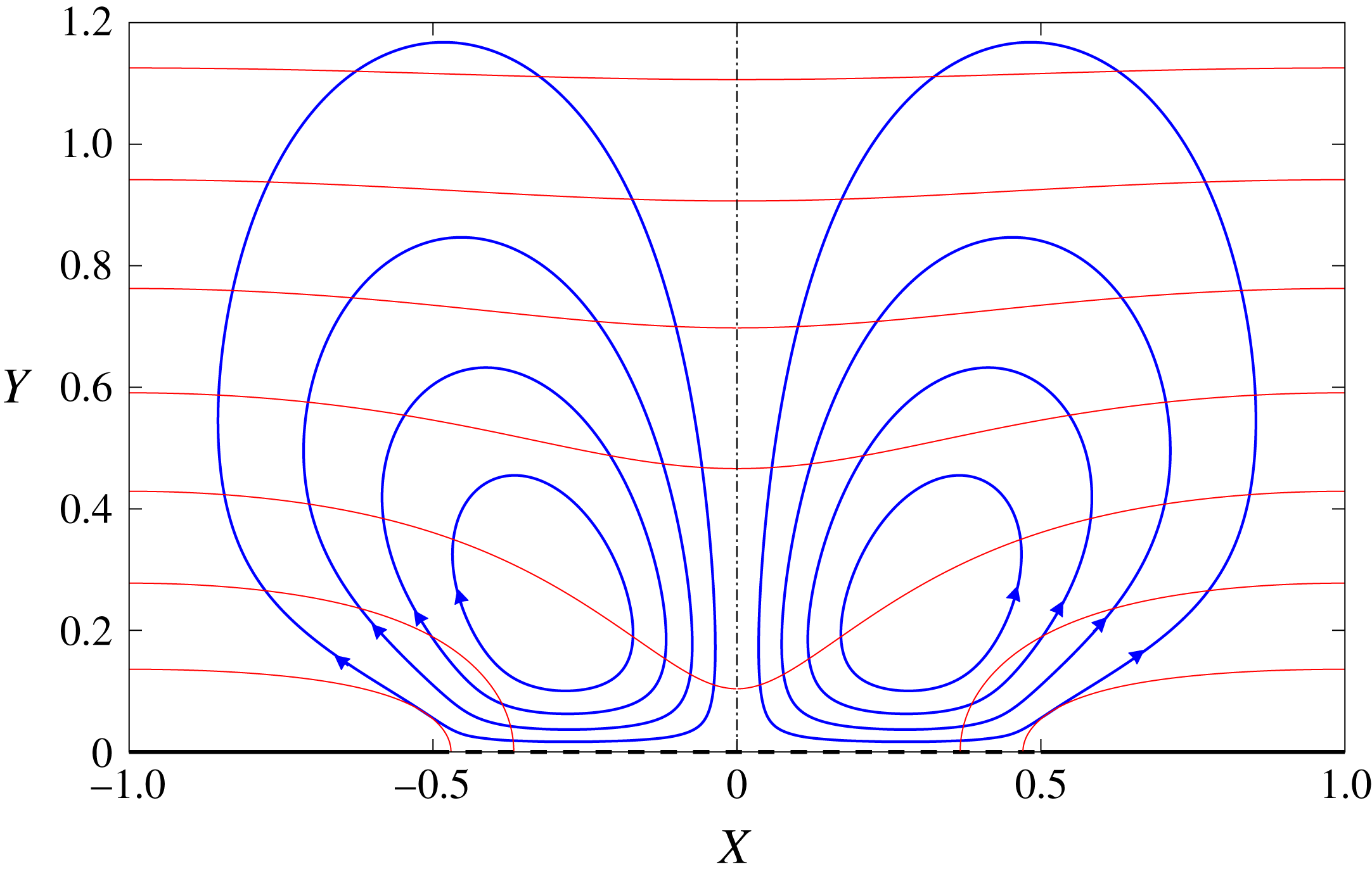
, are portrayed in figure 2 for
 $\unicode[STIX]{x1D6E5}=1/2$
. For reference, we also present in that figure the excess-temperature isotherms, obtained using (4.6) and (5.11).


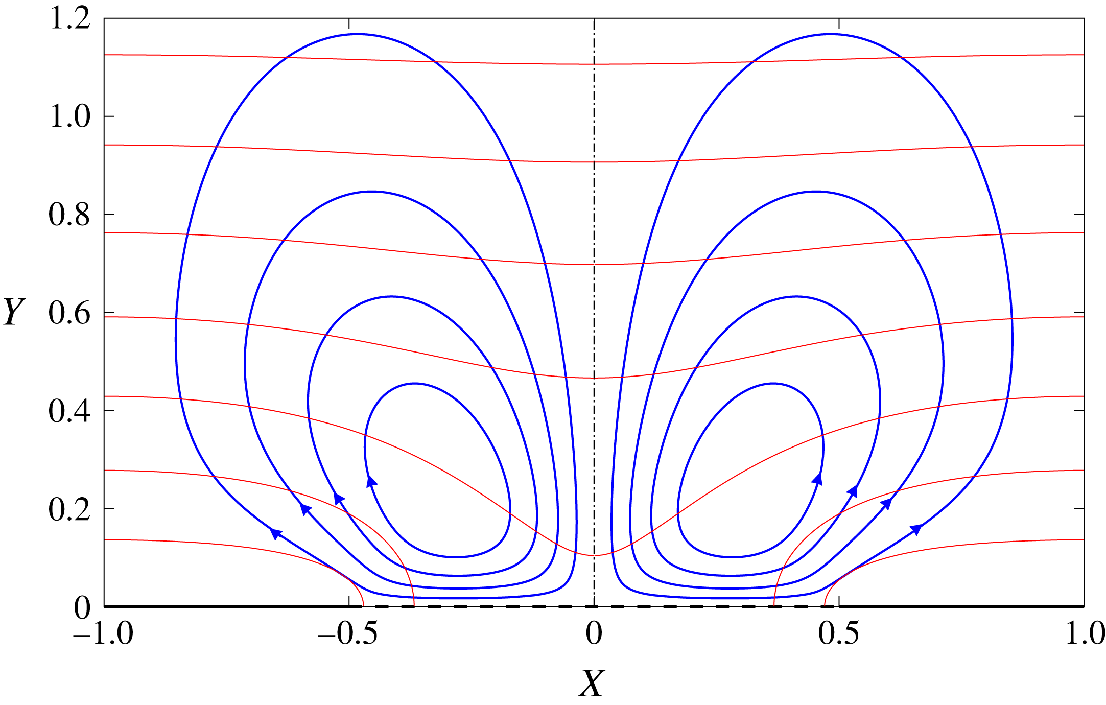
While the exponential decay in (5.21) guarantees that very few low-order modes are necessary for an accurate calculation of
 $\hat{\unicode[STIX]{x1D6F9}}$
, convergence in the determination of the respective Fourier coefficients is actually attained only for large
 $N$
, of approximately
 $10^{4}$
. This feature is typical of solutions to mixed boundary-value problems when solved by dual series methods: it has to do with the inherent square-root singularity associated with the transitions in (5.18) between two types of boundary condition. Since the series method does not explicitly account for this singularity, the matrix representing the algebraic equations governing
 $\{A_{n}\}_{n=1}^{\infty }$
is dense. It is plausible that alternative complex-variable approaches, which do account for the singularity explicitly (Crowdy Reference Crowdy2011, Reference Crowdy2013), may be employed to solve the problem posed by (5.16)–(5.20).
6 Large Marangoni numbers
When addressing the limit
 $\unicode[STIX]{x1D6EC}\rightarrow 0$
with
 $Ma=O(\unicode[STIX]{x1D6EC}^{-1})$
, it is convenient to write
 $$\begin{eqnarray}Ma=\unicode[STIX]{x1D6EC}^{-1}\widetilde{Ma}\end{eqnarray}$$
and to treat
 $\widetilde{Ma}$
as a fixed
 $O(1)$
parameter.
6.1 Outer region
Considering first heat transport in the outer region we note that the general observations made at the beginning of § 5 are independent of the Marangoni number scaling. Thus, both the leading-order term in the outer expansion of
 $\unicode[STIX]{x1D703}$
, as well as its two successive corrections (of relative magnitudes
 $\unicode[STIX]{x1D6EC}$
and
 $\unicode[STIX]{x1D6EC}^{2}$
) are independent of
 $X$
. The
 $O(\unicode[STIX]{x1D6EC}^{-1})$
large longitudinal advection in the energy balance (2.21) can be balanced by conduction in the
 $y$
-direction only if the excess-temperature variations are of the same order. We accordingly postulate the outer expansion
 $$\begin{eqnarray}\unicode[STIX]{x1D703}(x,y;\unicode[STIX]{x1D6EC})=\unicode[STIX]{x1D6EC}^{-1}\bar{\unicode[STIX]{x1D703}}(y)+\cdots \,,\end{eqnarray}$$
where the subsequent
 $O(1)$
and
 $O(\unicode[STIX]{x1D6EC})$
corrections are also independent of
 $X$
. At leading order, the advection–diffusion equation (2.21) then reads
 $$\begin{eqnarray}-\widetilde{Ma}\,\bar{w}=\frac{\text{d}^{2}\bar{\unicode[STIX]{x1D703}}}{\text{d}y^{2}}.\end{eqnarray}$$
Integration in conjunction with the symmetry condition (2.5) gives (cf. (5.5))
 $$\begin{eqnarray}\bar{\unicode[STIX]{x1D703}}=\frac{\widetilde{Ma}\,\bar{w}}{2}(1-y^{2}),\end{eqnarray}$$
where, just as in (5.5), the additive constant has been set so as to nullify
 $\bar{\unicode[STIX]{x1D703}}$
at
 $y=-1$
.
6.2 Dominant advection in the inner region?
Naively, following the methodology used in the case of moderate Marangoni numbers, one may conclude from heat-flux matching that
 $\unicode[STIX]{x1D703}=O(1)$
in the inner region,
 $$\begin{eqnarray}\unicode[STIX]{x1D703}(x,y;\unicode[STIX]{x1D6EC})=\unicode[STIX]{x1D6E9}(X,Y)+\cdots \,,\end{eqnarray}$$
whereby the Marangoni condition (2.18) implies that the cross-sectional flow there is
 $O(\unicode[STIX]{x1D6EC}^{-1})$
,
 $$\begin{eqnarray}u(x,y;\unicode[STIX]{x1D6EC})=\unicode[STIX]{x1D6EC}^{-1}U(X,Y)+\cdots \,,\quad v(x,y;\unicode[STIX]{x1D6EC})=\unicode[STIX]{x1D6EC}^{-1}V(X,Y)+\cdots \,.\end{eqnarray}$$
This scaling implies that
 $\unicode[STIX]{x1D6E9}$
is dominated by advection with the cross-sectional flow, namely
 $$\begin{eqnarray}\boldsymbol{U}\boldsymbol{\cdot }\unicode[STIX]{x1D735}_{\boldsymbol{X}}\unicode[STIX]{x1D6E9}=0,\end{eqnarray}$$
in which
 $$\begin{eqnarray}\boldsymbol{U}=\hat{\boldsymbol{e}}_{x}U+\hat{\boldsymbol{e}}_{y}V,\quad \unicode[STIX]{x1D735}_{\boldsymbol{X}}=\hat{\boldsymbol{e}}_{x}\frac{\unicode[STIX]{x2202}}{\unicode[STIX]{x2202}X}+\hat{\boldsymbol{e}}_{y}\frac{\unicode[STIX]{x2202}}{\unicode[STIX]{x2202}Y}.\end{eqnarray}$$
In addition to (6.7),
 $\unicode[STIX]{x1D6E9}$
is also governed by the homogeneous conditions (5.8) and (5.9), as well as the inhomogeneous flux-matching condition (cf. (5.10))
 $$\begin{eqnarray}\frac{\unicode[STIX]{x2202}\unicode[STIX]{x1D6E9}}{\unicode[STIX]{x2202}Y}\rightarrow \widetilde{Ma}\,\bar{w}\quad \text{as}~Y\rightarrow \infty .\end{eqnarray}$$
Equation (6.7) implies that
 $\unicode[STIX]{x1D6E9}$
is a constant on each of the cross-sectional ‘streamlines’ of
 $\boldsymbol{U}$
. This is alternatively written as
 $$\begin{eqnarray}\unicode[STIX]{x1D6E9}=f(\unicode[STIX]{x1D6F9}),\end{eqnarray}$$
wherein
 $\unicode[STIX]{x1D6F9}$
, the streamfunction associated with
 $\boldsymbol{U}$
, is defined as in (5.14). The different temperature scaling in the outer and inner regions excludes ‘open’ streamlines in the inner region (namely lines that reach the outer region). A closed-streamline structure, as in the case of moderate
 $Ma$
, is accordingly predicted. We now show that such a structure is inconsistent with (6.9), thus leading to a contradiction. The following arguments are based upon ideas devised in classical analyses of dominant advection along closed streamlines (Batchelor Reference Batchelor1956; Pan & Acrivos Reference Pan and Acrivos1968).
We start with the energy equation (2.4). Integrating over a two-dimensional domain
 ${\mathcal{D}}$
which lies entirely in the cross-sectional liquid domain yields, upon making use of the two-dimensional variant of Gauss’s theorem,
 $$\begin{eqnarray}\oint _{\unicode[STIX]{x2202}{\mathcal{D}}}\,\text{d}l\,\hat{\boldsymbol{n}}\boldsymbol{\cdot }(Ma\,\unicode[STIX]{x1D703}\,\boldsymbol{u}-\unicode[STIX]{x1D735}\unicode[STIX]{x1D703})=Ma\int _{{\mathcal{D}}}\,\text{d}x\,\text{d}y\,w,\end{eqnarray}$$
wherein
 $\unicode[STIX]{x2202}{\mathcal{D}}$
denotes the boundary of
 ${\mathcal{D}}$
,
 $\hat{\boldsymbol{n}}$
is an outward-pointing unit vector normal to
 $\unicode[STIX]{x2202}{\mathcal{D}}$
, and
 $\text{d}l$
is a differential length element. In particular, choosing
 ${\mathcal{D}}$
as the interior of an (arbitrary) streamline in the cross-sectional plane, for which
 $\hat{\boldsymbol{n}}\boldsymbol{\cdot }\boldsymbol{u}=0$
, gives
 $$\begin{eqnarray}-\!\oint _{\unicode[STIX]{x2202}{\mathcal{D}}}\,\text{d}l\,\hat{\boldsymbol{n}}\boldsymbol{\cdot }\unicode[STIX]{x1D735}\unicode[STIX]{x1D703}=Ma\int _{{\mathcal{D}}}\,\text{d}x\,\text{d}y\,w.\end{eqnarray}$$
The above relation is exact. We consider now the limit
 $\unicode[STIX]{x1D6EC}\rightarrow 0$
with the Marangoni-number scaling (6.1). Applying (6.12) to a closed streamline in the inner region, one obtains
 $$\begin{eqnarray}-\!\oint _{\unicode[STIX]{x2202}{\mathcal{D}}}\,\text{d}L\,\hat{\boldsymbol{n}}\boldsymbol{\cdot }\unicode[STIX]{x1D735}_{\boldsymbol{X}}(\unicode[STIX]{x1D6E9}+\cdots \!)=\unicode[STIX]{x1D6EC}\,\widetilde{Ma}\int _{{\mathcal{D}}}\,\text{d}X\,\text{d}Y\,(W+\cdots \,),\end{eqnarray}$$
where
 $\text{d}L=\unicode[STIX]{x1D6EC}^{-1}\,\text{d}l$
is a properly scaled differential length element. At leading order, where
 $\unicode[STIX]{x2202}{\mathcal{D}}$
coincides with an isoline of
 $\unicode[STIX]{x1D6F9}$
, we accordingly obtain
 $$\begin{eqnarray}\oint _{\unicode[STIX]{x1D6F9}=\text{const.}}\,\text{d}L\,\hat{\boldsymbol{n}}\boldsymbol{\cdot }\unicode[STIX]{x1D735}_{\boldsymbol{X}}\unicode[STIX]{x1D6E9}=0.\end{eqnarray}$$
At this stage it is convenient to employ
 $\unicode[STIX]{x1D6F9}$
itself as a curvilinear coordinate. The other curvilinear coordinate, say
 $\unicode[STIX]{x1D709}$
, is chosen such that
 $\unicode[STIX]{x1D6F9}$
and
 $\unicode[STIX]{x1D709}$
constitute a family of orthogonal coordinates. With that choice we have
 $$\begin{eqnarray}(\text{d}L)^{2}=h_{\unicode[STIX]{x1D6F9}}^{2}(\text{d}\unicode[STIX]{x1D6F9})^{2}+h_{\unicode[STIX]{x1D709}}^{2}(\text{d}\unicode[STIX]{x1D709})^{2},\end{eqnarray}$$
wherein
 $h_{\unicode[STIX]{x1D6F9}}$
and
 $h_{\unicode[STIX]{x1D709}}$
are the appropriate metric coefficients, which are generally functions of
 $\unicode[STIX]{x1D6F9}$
and
 $\unicode[STIX]{x1D709}$
. In particular, on the isoline
 $\unicode[STIX]{x1D6F9}=\text{const.}$
we have
 $\text{d}L=h_{\unicode[STIX]{x1D709}}|\text{d}\unicode[STIX]{x1D709}|$
, in which
 $h_{\unicode[STIX]{x1D709}}$
is a function of
 $\unicode[STIX]{x1D709}$
alone. Moreover, making use of (6.10) we find that
 $\hat{\boldsymbol{n}}\boldsymbol{\cdot }\unicode[STIX]{x1D735}_{\boldsymbol{X}}\unicode[STIX]{x1D6E9}=-(h_{\unicode[STIX]{x1D6F9}})^{-1}\,\text{d}\unicode[STIX]{x1D6E9}/\text{d}\unicode[STIX]{x1D6F9}$
on that curve. Substituting this expression into relation (6.14) and noting that
 $\text{d}\unicode[STIX]{x1D6E9}/\text{d}\unicode[STIX]{x1D6F9}$
may be taken out of the integral sign, we eventually obtain
 $$\begin{eqnarray}\frac{\text{d}\unicode[STIX]{x1D6E9}}{\text{d}\unicode[STIX]{x1D6F9}}\oint _{\unicode[STIX]{x1D6F9}=\text{const.}}|\text{d}\unicode[STIX]{x1D709}|\,\frac{h_{\unicode[STIX]{x1D709}}}{h_{\unicode[STIX]{x1D6F9}}}=0.\end{eqnarray}$$
Since both metric coefficients are positive, so must be the integral. It follows that
 $\text{d}\unicode[STIX]{x1D6E9}/\text{d}\unicode[STIX]{x1D6F9}=0$
on the curve
 $\unicode[STIX]{x1D6F9}=\text{const}$
. Since the constant is arbitrary, this is true for all closed streamlines and hence in the entire inner region. It follows that
 $\unicode[STIX]{x1D6E9}$
is uniform there. The said uniformity, however, is incompatible with (6.9). The preceding construction, starting with expansion (6.5), must be abandoned.
6.3 Nested boundary-layer structure
The presumed
 $O(\unicode[STIX]{x1D6EC})$
extent of the inner region was set by the unit-cell geometry. In postulating the naive expansion (6.5) we have assumed that the
 $\unicode[STIX]{x1D6EC}$
scale is relevant to the near-boundary transport in both the
 $x$
- and
 $y$
-directions. While this assumption is consistent at moderate Marangoni numbers, it fails at large Marangoni numbers. This suggests that the small scale pertinent to transport in the
 $y$
-direction, say
 $\unicode[STIX]{x1D6E5}$
, is determined in that case by a balance between advection and conduction, rather than by the geometry. (Owing to periodicity,
 $x$
-variations still take place on the
 $\unicode[STIX]{x1D6EC}$
scale.) Since the case
 $\unicode[STIX]{x1D6E5}=\unicode[STIX]{x1D6EC}$
resulted in dominant advection (see (6.7)), we anticipate that
 $\unicode[STIX]{x1D6E5}\ll \unicode[STIX]{x1D6EC}$
is needed for conduction to enter the dominant balance. It is important to note that the newly identified boundary layer is relevant only to the advection–diffusion equation governing
 $\unicode[STIX]{x1D703}$
: since the cross-sectional flow is coupled to
 $\unicode[STIX]{x1D703}$
only through the boundary condition (2.18) at
 $y=-1$
, it is ‘unaware’ of the existence of that layer. The velocity components
 $u$
and
 $v$
thus vary on the inner
 $\unicode[STIX]{x1D6EC}$
scale in both
 $x$
- and
 $y$
-directions.
We accordingly look for a dominant balance of the advection–diffusion equation (2.21). Balancing the
 $O(\unicode[STIX]{x1D6EC}^{-1})$
heat flux associated with the outer scaling (6.2) implies that the boundary-layer excess temperature is of order
 $\unicode[STIX]{x1D6E5}/\unicode[STIX]{x1D6EC}$
. The cross-sectional flow, driven by the Marangoni condition (2.18), is then of order
 $\unicode[STIX]{x1D6E5}/\unicode[STIX]{x1D6EC}^{2}$
. (Recall that
 $u$
varies on the scale
 $\unicode[STIX]{x1D6EC}$
, rather than
 $\unicode[STIX]{x1D6E5}$
.) Since
 $\unicode[STIX]{x1D6E5}\ll \unicode[STIX]{x1D6EC}$
, the conduction term in (2.21) is dominated by
 $y$
-derivatives, and is hence of order
 $(\unicode[STIX]{x1D6EC}\unicode[STIX]{x1D6E5})^{-1}$
. This term must be balanced by advective terms. With the Marangoni-number scaling (6.1), the longitudinal advection term in (2.21) is
 $O(\unicode[STIX]{x1D6EC}^{-1})$
, while the cross-sectional advection terms are of order
 $\unicode[STIX]{x1D6E5}^{2}/\unicode[STIX]{x1D6EC}^{5}$
. The only possible dominant balance is between conduction perpendicular to the surface and cross-sectional advection, giving
 $$\begin{eqnarray}\unicode[STIX]{x1D6E5}=\unicode[STIX]{x1D6EC}^{4/3},\end{eqnarray}$$
which is indeed much less than
 $\unicode[STIX]{x1D6EC}$
, as required. With both the conduction and cross-sectional advection terms in (2.21) being
 $O(\unicode[STIX]{x1D6EC}^{-7/3})$
, the
 $O(\unicode[STIX]{x1D6EC}^{-1})$
longitudinal advection term is subdominant.
We accordingly define the boundary-layer coordinate
 $$\begin{eqnarray}\unicode[STIX]{x1D702}=\frac{y+1}{\unicode[STIX]{x1D6EC}^{4/3}}\end{eqnarray}$$
and employ the associated boundary-layer expansion
 $$\begin{eqnarray}\unicode[STIX]{x1D703}(x,y;\unicode[STIX]{x1D6EC})=\unicode[STIX]{x1D6EC}^{1/3}\unicode[STIX]{x1D6E9}(X,\unicode[STIX]{x1D702})+\cdots \,.\end{eqnarray}$$
In addition, we employ the following expansions in the velocity components in the inner region, where they are functions of
 $X$
and
 $Y$
(cf. (5.12)),
 $$\begin{eqnarray}u(x,y;\unicode[STIX]{x1D6EC})=\unicode[STIX]{x1D6EC}^{-2/3}U(X,Y)+\cdots \!,\quad v(x,y;\unicode[STIX]{x1D6EC})=\unicode[STIX]{x1D6EC}^{-2/3}V(X,Y)+\cdots \,.\end{eqnarray}$$
At leading order, then, the advection–diffusion balance (2.21) reads:
 $$\begin{eqnarray}\widetilde{Ma}\left[U(X,0)\frac{\unicode[STIX]{x2202}\unicode[STIX]{x1D6E9}}{\unicode[STIX]{x2202}X}+\unicode[STIX]{x1D702}\frac{\unicode[STIX]{x2202}V}{\unicode[STIX]{x2202}Y}(X,0)\frac{\unicode[STIX]{x2202}\unicode[STIX]{x1D6E9}}{\unicode[STIX]{x2202}\unicode[STIX]{x1D702}}\right]=\frac{\unicode[STIX]{x2202}^{2}\unicode[STIX]{x1D6E9}}{\unicode[STIX]{x2202}\unicode[STIX]{x1D702}^{2}}.\end{eqnarray}$$
This equation is supplemented by the flux-matching condition,
 $$\begin{eqnarray}\frac{\unicode[STIX]{x2202}\unicode[STIX]{x1D6E9}}{\unicode[STIX]{x2202}\unicode[STIX]{x1D702}}\rightarrow \widetilde{Ma}\,\bar{w}\quad \text{as}~Y\rightarrow \infty ;\end{eqnarray}$$
the homogeneous conditions at
 $\unicode[STIX]{x1D702}=0$
,
 $$\begin{eqnarray}\frac{\unicode[STIX]{x2202}\unicode[STIX]{x1D6E9}}{\unicode[STIX]{x2202}\unicode[STIX]{x1D702}}=0\quad \text{for}~|X|<\unicode[STIX]{x1D6E5},\quad \unicode[STIX]{x1D6E9}=0\quad \text{for}~\unicode[STIX]{x1D6E5}<|X|<1;\end{eqnarray}$$
and the periodicity conditions,
 $$\begin{eqnarray}\frac{\unicode[STIX]{x2202}\unicode[STIX]{x1D6E9}}{\unicode[STIX]{x2202}X}=0\quad \text{at}~X=\pm 1.\end{eqnarray}$$
The equations governing the cross-sectional flow components follow from (2.14)–(2.20). They consist of: (i) the continuity and Stokes equations,
 $$\begin{eqnarray}\frac{\unicode[STIX]{x2202}U}{\unicode[STIX]{x2202}X}+\frac{\unicode[STIX]{x2202}V}{\unicode[STIX]{x2202}Y}=0,\quad \left(\frac{\unicode[STIX]{x2202}^{2}}{\unicode[STIX]{x2202}X^{2}}+\frac{\unicode[STIX]{x2202}^{2}}{\unicode[STIX]{x2202}Y^{2}}\right)\left(\frac{\unicode[STIX]{x2202}V}{\unicode[STIX]{x2202}X}-\frac{\unicode[STIX]{x2202}U}{\unicode[STIX]{x2202}Y}\right)=0;\end{eqnarray}$$
(ii) conditions at
 $Y=0$
, including impermeability and Marangoni forcing at the free surface,
 $$\begin{eqnarray}V=0,\quad \frac{\unicode[STIX]{x2202}U}{\unicode[STIX]{x2202}Y}=\frac{\unicode[STIX]{x2202}\unicode[STIX]{x1D6E9}}{\unicode[STIX]{x2202}X}\quad \text{for}~|X|<\unicode[STIX]{x1D6E5},\end{eqnarray}$$
as well as impermeability and no-slip conditions at the solid patches,
 $$\begin{eqnarray}U=V=0\quad \text{for}~\unicode[STIX]{x1D6E5}<|X|<1;\end{eqnarray}$$
(iii) the periodicity conditions,
 $$\begin{eqnarray}U=\frac{\unicode[STIX]{x2202}V}{\unicode[STIX]{x2202}X}=0\quad \text{at}~X=\pm 1;\end{eqnarray}$$
and (iv) large-
 $Y$
attenuation,
 $$\begin{eqnarray}U,V\rightarrow 0\quad \text{as}~Y\rightarrow \infty .\end{eqnarray}$$
Note that the derivative
 $\unicode[STIX]{x2202}\unicode[STIX]{x1D6E9}/\unicode[STIX]{x2202}X$
appearing in the Marangoni condition (6.26b
) is understood to be evaluated at
 $\unicode[STIX]{x1D702}=0$
(since
 $\unicode[STIX]{x1D6E9}$
is a function of
 $\unicode[STIX]{x1D702}$
, rather than
 $Y$
).
The flow and excess-temperature problems are mutually coupled through both (6.21) and (6.26b
). This coupling involves the distributions of the pertinent fields only at the respective boundaries
 $Y=0$
and
 $\unicode[STIX]{x1D702}=0$
. Unfortunately, the inherent nonlinearity in (6.21) appears to thwart the possibility of a closed-form solution. This nonlinearity also implies a complicated dependence of both the excess temperature and cross-sectional flow upon the Marangoni number.
7 Concluding remarks
This paper, which addresses longitudinal thermocapillary flows between grooved surfaces, provides two key contributions. The first, discussed in § 3, is the analogy between the longitudinal flow and that appearing in pressure-driven flow in the same geometry. This analogy is manifested in the general linkage (3.5) between the mean velocity in the two flows. The second contribution, which constitutes the majority of the paper (namely §§ 4–6), is concerned with the deep-channel limit. Notwithstanding the above-mentioned analogy, that limit reveals a qualitative difference between the temperature- and pressure-driven flow problems. Thus, while in the latter problem the conventional Poiseuille flow in the outer region drives the inner flow near the compound boundaries, in the present problem the uniform outer flow is animated by the Marangoni-generated flow within the inner regions. This difference is reflected in the superhydrophobic effect on the mean velocity: in the pressure-driven problem, it results in a small perturbation to the value associated with Poiseuille flow between two no-slip walls; in the present problem, where no flow occurs in the absence of superhydrophobic surfaces, this effect is dominant. (This is another aspect in which the analogy with electro-osmosis, discussed in § 1, is relevant.)
A natural extension of the present analysis involves the incorporation of non-zero protrusion angles, an extension that has been addressed extensively lately, in the context of mechanically driven flows (Crowdy Reference Crowdy2017; Marshall Reference Marshall2017). With a non-planar interface, condition (2.11) is modified to
 $$\begin{eqnarray}\frac{\unicode[STIX]{x2202}w}{\unicode[STIX]{x2202}\unicode[STIX]{x1D708}}=-\unicode[STIX]{x1D6EC}^{-1}\quad \text{for}~|x|<\unicode[STIX]{x1D6EC}\unicode[STIX]{x1D6E5},\end{eqnarray}$$
in which
 $\unicode[STIX]{x2202}/\unicode[STIX]{x2202}\unicode[STIX]{x1D708}$
denotes differentiation normal to the interface, in a direction pointing into the liquid. It is evident that (3.2) transforms (7.1) into a generally inhomogeneous condition governing
 $\unicode[STIX]{x2202}\grave{w} /\unicode[STIX]{x2202}\unicode[STIX]{x1D708}$
. Thus, in contrast to the plane-interface case (see (3.4a
)),
 $\grave{w}$
does not satisfy here the boundary conditions of the comparable pressure-driven flow problem. It is therefore unclear whether a general relation of the form (3.5) between temperature- and pressure-driven flows may be identified in the case of non-planar geometry.
Other possible extensions have to do with additional asymptotic limits, reflecting extreme values of the geometric parameters
 $\unicode[STIX]{x1D6EC}$
and
 $\unicode[STIX]{x1D6E5}$
. In particular, while the linkage (3.5) clearly indicates that the limits of shallow channels and small solid fractions are singular, it does not shed light on the underlying details of the longitudinal flow problems. Moreover, the singularities inherent in these problems suggest a rich structure of the accompanying coupled problem governing the temperature distribution and cross-sectional flow.
Yet another interesting extension may involve extreme values of the Marangoni numbers. In our analysis we have naturally encountered large Marangoni numbers as a by-product of the shallow-channel limit. One may consider, however, the limits of small and large Marangoni numbers independently. As explained in § 2.4, the case
 $Ma=0$
is rather trivial, thus suggesting the feasibility of a small-Marangoni-number analysis. The limit of large Marangoni number is singular, and is expected to result in non-trivial asymptotic scaling and flow topology (Balasubramaniam & Subramaniam Reference Balasubramaniam and Subramaniam1996; Balasubramaniam & Subramanian Reference Balasubramaniam and Subramanian2000).
In this paper we did not address the transverse problem, where the macroscopic temperature gradient is applied perpendicular to the grooves. This problem is conceptually different from the longitudinal one, since even under the assumption of highly conducting solid substrate the temperature distribution there must be solved for, a feature that introduces an awkward dependence upon the shape of the grooves which has no parallel in pressure-driven flow. In attempting to circumvent this difficulty, Baier et al. (Reference Baier, Steffes and Hardt2010) considered the case of ‘deep’ slats, where the temperature distribution at the solid–liquid interfaces is approximately piecewise uniform. Even under that assumption, however, the problem is significantly more complicated than the longitudinal one; thus, when addressing the deep-channel limit, Baier et al. (Reference Baier, Steffes and Hardt2010) had to resort to numerical computations in order to calculate the ‘far-field’ velocity in that problem. We are currently exploring the possibility of asymptotic analyses of the transverse-flow problem.
Acknowledgement
This work was supported by the Israel Science Foundation (grant no. 1081/16).