1 Introduction
Kinetic models are based on the description of the velocity distribution function for electrons and ions. An often-used approach is to describe this distribution statistically, employing a sample of particles: this is the particle-in-cell (PIC) method (Hockney & Eastwood Reference Hockney and Eastwood1988; Birdsall & Langdon Reference Birdsall and Langdon2004). A critical distinction within PIC methods is between explicit and implicit algorithms. Explicit algorithms alternatively move particles (in the fields known until that time) and advance the fields (with the sources provided by the particle velocity and position known until that time). This alternative advancing decouples the field and particle equations resulting in a very simple and highly computationally efficient technique. However, the explicit method is limited in what ranges of time steps and grid spacings it can use: the electron scales need to be resolved down to the smallest scales (Hockney & Eastwood Reference Hockney and Eastwood1988; Birdsall & Langdon Reference Birdsall and Langdon2004).
If the electron physics does not necessarily need to be resolved with great accuracy, the explicit method is not appropriate because the attempt to run the simulation with lower resolution is met first with an excessive numerical heating due to the failure of energy conservation, followed by numerical instability if the resolution is too coarse (Hockney & Eastwood Reference Hockney and Eastwood1988; Birdsall & Langdon Reference Birdsall and Langdon2004).
This limitation is eliminated by the implicit methods (Chen, Chacón & Barnes Reference Chen, Chacón and Barnes2011; Markidis & Lapenta Reference Markidis and Lapenta2011), where particles and fields are advanced together in a nonlinear iterative scheme. To remove the complexity of the nonlinear coupling and to reduce the computational cost per time step, semi-implicit methods have been invented (Brackbill & Cohen Reference Brackbill and Cohen1985). In this case, the coupling between particles and fields is approximated linearly and a self-consistent equation is solved for the fields alone without needing to iterate with the particles. Two previous semi-implicit classes of algorithms have been published: the direct implicit method (DIM) (Langdon, Cohen & Friedman Reference Langdon, Cohen and Friedman1983) based on expressing the particle response to field changes via a sensitivity matrix, and the implicit moment method (IMM) (Brackbill & Forslund Reference Brackbill and Forslund1982) based on approximating the plasma response using moments of the distribution function (typically up to the pressure tensor).
While implicit methods conserve energy exactly, semi-implicit methods tend to either lose or gain energy depending on the specifics of the configuration of the run (Cohen et al. Reference Cohen, Langdon, Hewett and Procassini1989). This lack of energy conservation results in a limiting of the range of resolution accessible. For example, in reconnection simulations (Lapenta Reference Lapenta2012) such as the one reported as an example here, the grid resolution needs to resolve the electron skin depth to represent the physics correctly, but it does not need to resolve the Debye length. Similarly, the particle trajectories need to be well resolved, a goal reached by resolving well the electron cyclotron motion, but the plasma frequency does not need to be resolved accurately. For low density, low temperature plasmas, there is a vast gap between the Debye- and skin-depth-scale. In these situations, the semi-implicit methods struggle to conserve energy at a sufficiently good degree to prevent numerical instability.
A new semi-implicit method has been recently developed to conserve energy exactly, to machine precision (Lapenta Reference Lapenta2016). The first published tests confirm exact energy conservation and suggest that when the method is applied to multiple-scale problems, the range of resolution where the method remains stable is wider than in previous semi-implicit schemes.
This possible beneficial effect is put to the test in the present paper, showing that for three examples of multiple-scale problems, the new method indeed allows us to cover a wide range of resolution without losing stability or energy conservation. First, we consider the ion acoustic wave, where both electron and ion physics play a role in the evolution and the method shows its ability to run resolving only the ion scales without artificially heating the electrons. Then, the electron acoustic instability is analysed. Here, the concurrent presence of three species: ions and cold and hot electrons, whose dynamics is characterized by different temporal and spatial scales, makes the problem multi-scale. In this case, we show that ECsim is able to capture the correct physics even when the smallest scales are not resolved. Finally, the well-known problem of the so-called geospace environmental modeling (GEM) challenge (Birn et al. Reference Birn, Drake, Shay, Rogers, Denton, Hesse, Kuznetsova, Ma, Bhattacharjee and Otto2001) is used to show that the only scales which need to be properly resolved are the electron skin depth in space and the cyclotron period in time (instead of the electron Debye length and the inverse of the electron frequency). Stepping over the smaller electron scales (Debye and plasma scales) does not lead to loss of energy conservation or stability even for cold rarefied plasmas where these scales are orders of magnitude smaller than the resolved scales.
2 Summary of the energy conserving semi-implicit PIC
Recently a new semi-implicit PIC method has been proposed to conserve energy exactly to machine precision (Lapenta Reference Lapenta2016). The fundamental enabling step that led to the new method is a new mover that allows for the explicit analytical calculation of the current generated by the particles during one time step without any approximation.
2.1 Particle mover
The new mover combines the DIM
 $D_{1}$
scheme (Hewett & Langdon Reference Hewett and Langdon1987) with the IMM and energy conserving particle in cell (ECPIC)
 $\unicode[STIX]{x1D703}$
-scheme (Brackbill & Forslund Reference Brackbill and Forslund1982). The particle position is advanced as in the
 $D_{1}$
scheme, but the velocity is advanced as in the
 $\unicode[STIX]{x1D703}$
scheme:
 $$\begin{eqnarray}\left.\begin{array}{@{}c@{}}\displaystyle \boldsymbol{x}_{p}^{n+1/2}=\boldsymbol{x}_{p}^{n-1/2}+\unicode[STIX]{x0394}t\boldsymbol{v}_{p}^{n},\\ \displaystyle \boldsymbol{v}_{p}^{n+1}=\boldsymbol{v}_{p}^{n}+\frac{q_{p}\unicode[STIX]{x0394}t}{m_{p}}(\boldsymbol{E}^{n+\unicode[STIX]{x1D703}}(\boldsymbol{x}_{p}^{n+1/2})+\overline{\boldsymbol{v}}_{p}\times \boldsymbol{B}^{n}(\boldsymbol{x}_{p}^{n+1/2})),\end{array}\right\}\end{eqnarray}$$
where
 $\overline{\boldsymbol{v}}_{p}=(\boldsymbol{v}_{p}^{n+1}+\boldsymbol{v}_{p}^{n})/2$
,
 $\unicode[STIX]{x0394}t$
is the time step,
 $q_{p}$
(
 $m_{p}$
) is the particle charge (mass) and
 $\boldsymbol{x}_{p}$
(
 $\boldsymbol{v}_{p}$
) is the particle position (velocity) of particle
 $p$
at the time level indicated by the superscript,
 $\boldsymbol{E}_{p}$
(
 $\boldsymbol{B}_{p}$
) is the electric (magnetic) field computed at the position of particle
 $p$
and the time level indicated by the superscript.
We evaluate the fields at the time staggered particle position
 $\boldsymbol{x}_{p}^{n+1/2}$
known explicitly from the time staggering of the leap-frog, but we use the implicit electric field at the
 $\unicode[STIX]{x1D703}$
time level:
 $\boldsymbol{E}^{n+\unicode[STIX]{x1D703}}$
as in the standard IMM. The fields are computed at the known position
 $\boldsymbol{x}_{p}^{n+1/2}$
rather than at the unknown position
 $\overline{\boldsymbol{x}}_{p}$
that in the standard IMM requires the predictor–corrector iteration. These two positions are conceptually similar, expressing the particle position at the mid-time between the old and new evaluations of the velocity. But one is computed explicitly while the other is computed as part of a predictor–corrector iteration. Both are second-order accurate, but the scheme in (2.1) is simpler to compute. The combined scheme is second-order accurate and has the same stability properties of the IMM. This property allows one to write the scheme to be exactly energy conserving.
The equation for the velocity can be solved analytically to express explicitly
 $\overline{\boldsymbol{v}}_{p}$
(Vu & Brackbill Reference Vu and Brackbill1992). Using vector manipulation, the velocity equation can be rewritten in the equivalent form:
 $$\begin{eqnarray}\overline{\boldsymbol{v}}_{p}=\widehat{\boldsymbol{v}}_{p}+\unicode[STIX]{x1D6FD}_{s}\widehat{\boldsymbol{E}}_{p},\end{eqnarray}$$
where hatted quantities have been rotated by the magnetic field:
 $$\begin{eqnarray}\left.\begin{array}{@{}c@{}}\widehat{\boldsymbol{v}}_{p}=\unicode[STIX]{x1D6FC}_{p}^{n}\boldsymbol{v}_{p}^{n},\\ \widehat{\boldsymbol{E}}_{p}=\unicode[STIX]{x1D6FC}_{p}^{n}\boldsymbol{E}_{p}^{n+\unicode[STIX]{x1D703}}\end{array}\right\}\end{eqnarray}$$
via a rotation matrix
 $\unicode[STIX]{x1D6FC}_{p}^{n}$
defined as:
 $$\begin{eqnarray}\unicode[STIX]{x1D6FC}_{p}^{n}=\frac{1}{1+(\unicode[STIX]{x1D6FD}_{s}B_{p}^{n})^{2}}(\unicode[STIX]{x1D644}-\unicode[STIX]{x1D6FD}_{s}\unicode[STIX]{x1D644}\times \boldsymbol{B}_{p}^{n}+\unicode[STIX]{x1D6FD}_{s}^{2}\boldsymbol{B}_{p}^{n}\boldsymbol{B}_{p}^{n}),\end{eqnarray}$$
where
 $\unicode[STIX]{x1D644}$
is the dyadic tensor (matrix with diagonal of 1) and
 $\unicode[STIX]{x1D6FD}_{s}=q_{p}\unicode[STIX]{x0394}t/2m_{p}$
(independent of the particle weight and unique to a given species).
The fields at the particle positions are computed by interpolation:
 $$\begin{eqnarray}\displaystyle & \displaystyle \boldsymbol{E}_{p}^{n+\unicode[STIX]{x1D703}}=\mathop{\sum }_{g}\boldsymbol{E}_{g}^{n+\unicode[STIX]{x1D703}}W(\boldsymbol{x}_{p}^{n+1/2}-\boldsymbol{x}_{g}), & \displaystyle\end{eqnarray}$$
 $$\begin{eqnarray}\displaystyle & \displaystyle \boldsymbol{B}_{p}^{n}=\mathop{\sum }_{g}\boldsymbol{B}_{g}^{n}W(\boldsymbol{x}_{p}^{n+1/2}-\boldsymbol{x}_{g}), & \displaystyle\end{eqnarray}$$
where we have assumed that the field equations are discretized on a grid with a generic index
 $g$
. For brevity we introduced the notation:
 $\boldsymbol{B}_{p}^{n}=\boldsymbol{B}^{n+\unicode[STIX]{x1D703}}(\boldsymbol{x}_{p}^{n+1/2})$
and
 $\boldsymbol{E}_{p}^{n+\unicode[STIX]{x1D703}}=\boldsymbol{E}^{n+\unicode[STIX]{x1D703}}(\boldsymbol{x}_{p}^{n+1/2})$
. In the examples below, the interpolation functions
 $W$
are
 $b$
-splines of order
 $\ell =1$
(De Boor Reference De Boor1978).
2.2 Field solver
For the Maxwell’s equations we use the same discretization as in the standard IMM (Markidis, Lapenta & Rizwan-uddin Reference Markidis and Lapenta2010). The two curl Maxwell’s equations are discretized in time with another
 $\unicode[STIX]{x1D703}$
scheme:
 $$\begin{eqnarray}\left.\begin{array}{@{}c@{}}\displaystyle \unicode[STIX]{x1D735}_{g}\times \boldsymbol{E}^{n+\unicode[STIX]{x1D703}}+\frac{1}{c}\frac{\boldsymbol{B}_{g}^{n+1}-\boldsymbol{B}_{g}^{n}}{\unicode[STIX]{x0394}t}=0,\\ \displaystyle \unicode[STIX]{x1D735}_{g}\times \boldsymbol{B}^{n+\unicode[STIX]{x1D703}}-\frac{1}{c}\frac{\boldsymbol{E}_{g}^{n+1}-\boldsymbol{E}_{g}^{n}}{\unicode[STIX]{x0394}t}=\frac{4\unicode[STIX]{x03C0}}{c}\overline{\boldsymbol{J}}_{g},\end{array}\right\}\end{eqnarray}$$
where
 $\overline{\boldsymbol{J}}_{g}$
is computed at the mid-temporal location. For each species we use
 $$\begin{eqnarray}\overline{\boldsymbol{J}}_{sg}=\frac{1}{V_{g}}\mathop{\sum }_{p}q_{p}\overline{\boldsymbol{v}}_{p}W(\boldsymbol{x}_{p}^{n+1/2}-\boldsymbol{x}_{g}),\end{eqnarray}$$
where the summation is over the particles of the same species, labelled by
 $s$
, and
 $W$
is the interpolation function. The total current is obtained summing over the species.
The spatial operators in (2.7) are discretized on a grid, indicating
 $\unicode[STIX]{x1D735}_{g}$
as a shorthand for the spatial discretization of the operators. In the examples below the same discretization as iPic3D is used (Sulsky & Brackbill Reference Sulsky and Brackbill1991; Markidis et al.
Reference Markidis and Lapenta2010; Lapenta Reference Lapenta2012), however, all the derivations below are not critically dependent on which spatial discretization is used.
2.3 Current evaluation
The set of Maxwell’s and Newton’s equations are coupled. In the spirit of the semi-implicit method, we do not want to solve two coupled sets with a single nonlinear iteration and find instead a way to extract analytically from the equations of motion the information needed for computing the current without first moving the particles. In previous semi-implicit methods this is done via a linearization procedure. The new mover used here allows us, instead, to derive the current rigorously without any approximation.
Substituting then (2.2) into (2.8), we obtain without any approximation or linearization:
 $$\begin{eqnarray}\overline{\boldsymbol{J}}_{sg}=\widehat{\boldsymbol{J}}_{sg}+\frac{\unicode[STIX]{x1D6FD}_{s}}{V_{g}}\mathop{\sum }_{p}q_{p}\unicode[STIX]{x1D6FC}_{p}^{n}\boldsymbol{E}_{p}^{n+\unicode[STIX]{x1D703}}W_{pg},\end{eqnarray}$$
where we have shortened the notation
 $W_{pg}=W(\boldsymbol{x}_{p}^{n+1/2}-\boldsymbol{x}_{g})$
and the summation is intended over all particles of species
 $s$
.
The following hatted currents were defined:
 $$\begin{eqnarray}\widehat{\boldsymbol{J}}_{sg}=\mathop{\sum }_{p}q_{p}\widehat{\boldsymbol{v}}_{p}W_{pg},\end{eqnarray}$$
representing the current based on the hatted velocities.
Computing then the electric field on the particles by interpolation from the grid as in (2.6), (2.9) becomes:
 $$\begin{eqnarray}\overline{\boldsymbol{J}}_{sg}=\widehat{\boldsymbol{J}}_{sg}+\frac{\unicode[STIX]{x1D6FD}_{s}}{V_{g}}\mathop{\sum }_{p}\mathop{\sum }_{g^{\prime }}q_{p}\unicode[STIX]{x1D6FC}_{p}^{n}\boldsymbol{E}_{g^{\prime }}^{n+\unicode[STIX]{x1D703}}W_{pg^{\prime }}W_{pg}.\end{eqnarray}$$
The formula above is conveniently expressed introducing mass matrices (Burgess, Sulsky & Brackbill Reference Burgess, Sulsky and Brackbill1992) defined by elements as
 $$\begin{eqnarray}\unicode[STIX]{x1D614}_{s,gg^{\prime }}^{ij}=\mathop{\sum }_{p}q_{p}\unicode[STIX]{x1D6FC}_{p}^{ij,n}W_{pg^{\prime }}W_{pg}.\end{eqnarray}$$
There are
 $3v$
such matrices, where
 $v$
is the dimensionality of the magnetic field and velocity vector, not to be confused with the dimensionality of the geometry used for space
 $d$
. The indices
 $i$
and
 $j$
in (2.12) vary in the
 $3v$
-space. For example, for full 3-component vectors,
 $i,j=1,2,3$
and there are 9 mass matrices. Each matrix is symmetric and very sparse with just
 $2d$
diagonals. In matrix notation the
 $3v$
mass matrices defined above are written as
 $\unicode[STIX]{x1D614}_{gg^{\prime }}$
, i.e. without the indices
 $i,j$
for the vector directions.
Using the mass matrices, the current becomes:
 $$\begin{eqnarray}\overline{\boldsymbol{J}}_{sg}=\widehat{\boldsymbol{J}}_{sg}+\frac{\unicode[STIX]{x1D6FD}_{s}}{V_{g}}\mathop{\sum }_{g^{\prime }}\unicode[STIX]{x1D614}_{s,gg^{\prime }}\boldsymbol{E}_{g^{\prime }}^{n+\unicode[STIX]{x1D703}}.\end{eqnarray}$$
Equation (2.13) is the central ingredient of the ECsim method: it expresses the advanced current at the mid-point of the time step and the electric field at the advanced time. This linear relationship can be substituted into the discretized Maxwell’s equations (2.7) to form a linear set of equations to be solved on the grid:
 $$\begin{eqnarray}\left.\begin{array}{@{}c@{}}\displaystyle \unicode[STIX]{x1D735}_{g}\times \boldsymbol{E}^{n+\unicode[STIX]{x1D703}}+\frac{1}{c}\frac{\boldsymbol{B}^{n+1}-\boldsymbol{B}^{n}}{\unicode[STIX]{x0394}t}=0,\\ \displaystyle \unicode[STIX]{x1D735}_{g}\times \boldsymbol{B}^{n+\unicode[STIX]{x1D703}}-\frac{1}{c}\frac{\boldsymbol{E}^{n+1}-\boldsymbol{E}^{n}}{\unicode[STIX]{x0394}t}=\frac{4\unicode[STIX]{x03C0}}{c}\left(\widehat{\boldsymbol{J}}_{g}+\mathop{\sum }_{g^{\prime }}\unicode[STIX]{x1D614}_{gg^{\prime }}\boldsymbol{E}_{g^{\prime }}^{n+\unicode[STIX]{x1D703}}\right),\end{array}\right\}\end{eqnarray}$$
where we have introduced the total current
 $\widehat{\boldsymbol{J}}_{g}=\sum _{s}\widehat{\boldsymbol{J}}_{sg}$
and the species summed mass matrices that written by elements are:
 $$\begin{eqnarray}\unicode[STIX]{x1D614}_{gg^{\prime }}^{ij}=\mathop{\sum }_{s}\frac{\unicode[STIX]{x1D6FD}_{s}}{V_{g}}\unicode[STIX]{x1D614}_{s,gg^{\prime }}^{ij},\end{eqnarray}$$
which can be more usefully held in memory, reducing the memory consumption by a factor equal to the number of species.
2.4 Energy conservation
The method described above, in the specific case
 $\unicode[STIX]{x1D703}=1/2$
, satisfies an exact energy conservation principle proven in Lapenta (Reference Lapenta2016):
 $$\begin{eqnarray}\displaystyle & & \displaystyle \displaystyle \mathop{\sum }_{g}\frac{(\boldsymbol{B}_{g}^{n+1})^{2}-(\boldsymbol{B}_{g}^{n})^{2}}{4\unicode[STIX]{x03C0}}+\mathop{\sum }_{g}\frac{(\boldsymbol{E}_{g}^{n+1})^{2}-(\boldsymbol{E}_{g}^{n})^{2}}{4\unicode[STIX]{x03C0}}\nonumber\\ \displaystyle & & \displaystyle \quad =\displaystyle \unicode[STIX]{x0394}t\mathop{\sum }_{g}\overline{\boldsymbol{J}}_{g}\boldsymbol{\cdot }\overline{\boldsymbol{E}}_{g}+\frac{c\unicode[STIX]{x0394}t}{4\unicode[STIX]{x03C0}}\mathop{\sum }_{g}\unicode[STIX]{x1D735}_{g}\boldsymbol{\cdot }(\boldsymbol{E}_{g}\times \boldsymbol{B}_{g}).\end{eqnarray}$$
The left-hand side is recognized as the variation of the magnetic and electric energy. The first term on the right-hand side is the energy exchange term with the particles and the last term is the divergence of the Poynting flux. This is the usual equation for electromagnetic energy conservation.
The examples below will further confirm in practice the validity of the result above, energy is conserved to machine precision.
3 Massively parallel implementation
The new ECsim has been implemented in a parallel code, which was built over the very basic structure of the implicit moment PIC code iPic3D (Markidis et al. Reference Markidis and Lapenta2010). Despite the differences between the algorithm used in iPic3D and the one presented here, there are many modules of iPic3D that could be retained in the new code, such as the particle communications between processors or the input/output procedure. As with its predecessor, the new code has been written in C and C++ and it uses message passing interface (MPI) for parallel communication between processes.
Similarly to iPic3D, the new code uses a three-dimensional Cartesian grid to compute the fields where the particles are immersed. When several processors are used, the physical domain is divided into subdomains. In order to compute the derivatives, each process not only owns one subdomain, but also the first cells of its neighbours (ghost cells). Those ghost values are communicated between processes through MPI routines. Analogously, each process owns the particles, which belong to its domain. After every cycle, the particles that have left the subdomain are communicated to the right process via MPI routines. The results of the simulation are written on disk using the HDF5 format for fields and particles, and in ASCII for other additional data (as the energy of the system or the input data used). Except for that, everything is different in the new code: the moment gathering, the field solver and the particle mover.
In order to solve the field equations (2.14), the implicit current and the mass matrices need to be computed in advance. The calculation of the implicit current is different from what was done in iPic3D. Here, for each particle it is necessary to interpolate the magnetic field from the grid to the particle position, then compute the
 $\unicode[STIX]{x1D6FC}$
matrix and once the implicit current for that particle has been calculated, interpolate it to the grid. The mass matrices were not present in iPic3D, and their calculation is the most time consuming part of the code. For each node there are 27 three-by-three mass matrices (
 $g^{\prime }$
can take the value of
 $g$
and all the neighbours nodes). However, due to their symmetry (
 $\unicode[STIX]{x1D614}_{gp}\equiv \unicode[STIX]{x1D614}_{pg}$
), only 14 matrices must be stored in memory for each node, which means that 126 scalar values have to be computed for each node.
In the ECsim algorithm both the electric and the magnetic fields are solved together whereas in iPic3D, first the electric field is obtained and then the magnetic field is computed as the curl of the electric field. Thus the linear system is twice as big as the one in iPic3D. For this reason we decided to use PETSc (Balay et al. Reference Balay, Abhyankar, Adams, Brown, Brune, Buschelman, Dalcin, Eijkhout, Gropp and Kaushik2016) for the task. PETSc is a suite of libraries which provide several tools to deal with problems ruled by differential equations. The main advantages of PETSc are that it is specially intended for parallel calculations, meaning that it should scale well when using many cores, and it allows the user to change between several linear and nonlinear solvers very easily.
Finally, once the fields are known, the positions and the velocities of the particles can be updated. Unlike what happens in iPic3D, here the mover has an explicit scheme (no iterations are needed). However, for each particle, the
 $\unicode[STIX]{x1D6FC}$
matrix needs to be computed. Note that this matrix was calculated in the moment gathering, but due to the high number of particles usually employed in the simulations, it is not practical to store these matrices in memory. Instead, the
 $\unicode[STIX]{x1D6FC}$
matrix is computed again for each particle. This implies the interpolation of both the electric and magnetic fields from the grid to the particles. Despite this fact, the particle mover in this code is much simpler than it was in iPic3D and it is less time consuming.
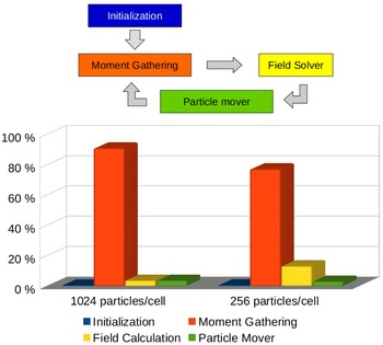
Main loop of the ECsim and the percentage of the total time spent in each task in two cases: with 1024 and 256 particles per cell.

In figure 1 the scheme of the main loop and the percentage of the total time spent in each task are shown. The data correspond to two different simulations of magnetic reconnection. In both cases, the domain was discretised in
 $256\times 128$
cells and the time step considered was
 $\unicode[STIX]{x0394}t=0.1\,\unicode[STIX]{x1D714}_{pi}^{-1}$
. A different number of particles per cell has been employed in the two simulations: 256 and 1024. Both tests have been carried out with 16 MPI processes in a single node with an Intel Xeon Sandy Bridge E5-2680 processor. The most time consuming portion of the code is the moment gathering; in particular, the calculation of the mass matrices is clearly the dominant part. As the number of particles decreases, we would expect the field solver time to become more important, however, even with only 256 particles per cell, the moment gathering is still the most time consuming part of the code. In all the tests performed, the time required by the particle mover is always negligible when compared with the moment gathering. Taking this into account, the optimization of the code should be focused on the moment gathering stage, and in particular on the mass matrix calculation. For instance, the vectorization of the mass matrix calculation (the field interpolation between the grid and the particles and the calculation of the elements of the mass matrices) will dramatically improve the performance. Future work will address this aspect.
Regarding the computation time required by the new code, if we analyse the time per cycle (with the same input values) ECsim is more time consuming than iPic3D (it takes approximately 3 times longer). However, if we look at the big picture, taking into account the fact that in the new code the time step can be chosen much larger than in iPic3D, the new code will need less cycles to cover the same physical time than iPic3D, and hence the total time of the simulation will be considerably reduced. Moreover, the grid size (i.e. the number of cells) is no longer a constraint. This means that if we are not interested in the smallest scales of the problem, we can use larger cells (i.e. less cells) and then reduce the time needed for each cycle.
4 Results
4.1 Ion acoustic wave
Ion acoustic waves are longitudinal low frequency modes, where both the ion and the electron dynamics play a role (Gary Reference Gary2005). Therefore, they represent an optimum multi-scale test for the ECsim algorithm. The wave is triggered by a density perturbation in a plasma composed of hot electrons and relatively colder ions. Considering Maxwellian electrons and ions with temperature
 $T_{e}$
and
 $T_{i}\ll T_{e}$
respectively, the wave dispersion relation is (Gary Reference Gary2005)
 $$\begin{eqnarray}\unicode[STIX]{x1D716}(\unicode[STIX]{x1D714},k)=1+\unicode[STIX]{x1D712}_{e}(\unicode[STIX]{x1D714},k)+\unicode[STIX]{x1D712}_{i}(\unicode[STIX]{x1D714},k),\end{eqnarray}$$
with the susceptibilities
 $\unicode[STIX]{x1D712}_{j}(\unicode[STIX]{x1D714},k)$
given by
 $$\begin{eqnarray}\unicode[STIX]{x1D712}_{j}(\unicode[STIX]{x1D714},k)=\frac{\unicode[STIX]{x1D714}_{pj}^{2}}{k^{2}v_{th,j}^{2}}\left[1+\frac{\unicode[STIX]{x1D714}}{\sqrt{2}kv_{th,j}}Z\left(\frac{\unicode[STIX]{x1D714}}{\sqrt{2}kv_{th,j}}\right)\right],\end{eqnarray}$$
where the subscript
 $j$
has been used to indicate the
 $j$
th species,
 $\unicode[STIX]{x1D714}\ll \unicode[STIX]{x1D714}_{pe}$
and
 $k$
are the wave frequency and the wavenumber respectively,
 $\unicode[STIX]{x1D714}_{pj}=\sqrt{4\unicode[STIX]{x03C0}e^{2}n_{j}/m_{j}}$
is the plasma frequency of the
 $j$
th species having density
 $n_{j}$
and mass
 $m_{j}$
,
 $e$
is the elementary charge,
 $v_{th,j}=\sqrt{T_{j}/m_{j}}$
is the thermal speed and
 $Z$
is the plasma dispersion function (Fried & Conte Reference Fried and Conte1961).
A series of numerical simulations were performed to check the code stability and accuracy. Similar parameters to those in Chen et al. (Reference Chen, Chacón and Barnes2011) have been used. A homogeneous plasma composed of electrons and ions with a reduced mass-to-charge ratio of 200 was introduced. Hot electrons with
 $T_{e}=20~\text{KeV}$
and ions with
 $T_{i}=2~\text{eV}$
were considered. At
 $t=0$
, a small sinusoidal perturbation was superimposed on the equilibrium density
 $n_{0}$
:
 $$\begin{eqnarray}n_{j}(t=0)=n_{0}\left[1+0.2\cos \left(\frac{2\unicode[STIX]{x03C0}}{L}x\right)\right],\end{eqnarray}$$
where
 $L=0.14\,c/\unicode[STIX]{x1D714}_{pi}$
is the simulation box length,
 $c$
is the speed of light in vacuum,
 $\unicode[STIX]{x1D714}_{pi}=\sqrt{4\unicode[STIX]{x03C0}e^{2}n_{0}/m_{i}}$
is the ion plasma frequency and
 $x$
is the longitudinal coordinate. The simulation box was discretised using 32 cells, so that
 $\unicode[STIX]{x0394}x\simeq 0.3\,\unicode[STIX]{x1D706}_{D}$
, with
 $\unicode[STIX]{x1D706}_{D}=\sqrt{T_{e}/4\unicode[STIX]{x03C0}e^{2}n_{0}}$
electron Debye length. All the simulations used 32 000 particles per species, which were pushed until
 $t_{end}\simeq 100\,\unicode[STIX]{x1D714}_{pi}^{-1}$
.
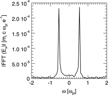
Frequency domain Fourier transform of the electric field component corresponding to
 $k=2\unicode[STIX]{x03C0}/L=45\,\unicode[STIX]{x1D714}_{pi}/c$
. FFT stands for Fourier transform. The peaks are located at
 $\unicode[STIX]{x1D714}=\pm 0.5\,\unicode[STIX]{x1D714}_{pi}$
, in perfect agreement with the solution of (4.1).

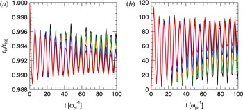
Evolution of the electron (a) and ion (b) kinetic energy for
 $\unicode[STIX]{x0394}t=0.0043$
(black), 0.0089 (green), 0.01 (orange), 0.0133 (blue) and 0.0177 (red)
 $\unicode[STIX]{x1D714}_{pi}^{-1}$
.

At first, code results have been compared with theory. In this case, a time step
 $\unicode[STIX]{x0394}t=0.0043\,\unicode[STIX]{x1D714}_{pi}^{-1}$
was employed. It is important to notice that this time step corresponds to the maximum value that can be used in an explicit electromagnetic PIC algorithm for stability reasons (
 $\unicode[STIX]{x0394}t_{\mathit{explicit}}<\unicode[STIX]{x0394}x/c$
). Figure 2 shows the Fourier transform in the frequency domain of the electric field. The field component corresponding to the excited mode
 $k=2\unicode[STIX]{x03C0}/L=45\,\unicode[STIX]{x1D714}_{pi}/c$
is displayed. The peaks correspond to a wave frequency
 $\unicode[STIX]{x1D714}=\pm 0.5\,\unicode[STIX]{x1D714}_{pi}$
, in perfect agreement with the solution of (4.1). A detailed study was performed increasing progressively the time step until the semi-implicit limit
 $\unicode[STIX]{x0394}t_{\mathit{implicit}}<\unicode[STIX]{x0394}x/v_{th,e}$
. Results are summarised in figure 3, where the evolution of the ion and electron kinetic energy is shown. In all the cases considered here, the long-term behaviour of the ion acoustic wave is well described. A stronger damping of the wave is observed when increasing the
 $\unicode[STIX]{x0394}t$
(Brackbill & Forslund Reference Brackbill and Forslund1982), but results are overall convergent and the physics of the wave is captured correctly, even when a big
 $\unicode[STIX]{x0394}t$
is chosen. In all the simulations, the total energy is conserved down to round-off precision as demonstrated in § 2.4.
4.2 Electron acoustic instability
In a plasma where ions are at rest and two different populations of electrons with similar density, but different temperature, are streaming against each other, when the relative drift is greater than the thermal velocity of the colder species, the electron acoustic instability may arise. The dispersion relation of the instability is given by (Gary Reference Gary2005)
 $$\begin{eqnarray}\unicode[STIX]{x1D716}(\unicode[STIX]{x1D714},k)=1+\unicode[STIX]{x1D712}_{c}(\unicode[STIX]{x1D714},k)+\unicode[STIX]{x1D712}_{h}(\unicode[STIX]{x1D714},k)+\unicode[STIX]{x1D712}_{i}(\unicode[STIX]{x1D714},k),\end{eqnarray}$$
where the subscripts
 $c$
,
 $h$
and
 $i$
indicate cold electrons, hot electrons and ions, respectively. If Maxwellian particles are considered, the ion susceptibility can be expressed by (4.2), while the electron susceptibilities are
 $$\begin{eqnarray}\unicode[STIX]{x1D712}_{j}(\unicode[STIX]{x1D714},k)=\frac{\unicode[STIX]{x1D714}_{pj}^{2}}{k^{2}v_{th,j}^{2}}\left[1+\frac{\unicode[STIX]{x1D714}+kv_{0,j}}{\sqrt{2}kv_{th,j}}Z\left(\frac{\unicode[STIX]{x1D714}+kv_{0,j}}{\sqrt{2}kv_{th,j}}\right)\right],\end{eqnarray}$$
with
 $j=c,h$
and
 $v_{0,j}$
the drift velocity.
Since
 $\unicode[STIX]{x1D706}_{Dc}\ll \unicode[STIX]{x1D706}_{Dh}$
and
 $\unicode[STIX]{x1D6E4}_{max}\ll \unicode[STIX]{x1D714}_{ph}\ll \unicode[STIX]{x1D714}_{pc}$
, where
 $\unicode[STIX]{x1D6E4}_{max}$
is the maximum growth rate of the instability, the electron acoustic instability represents a good multi-scale test for the ECsim algorithm. A simulation box with length
 $L=0.334\,c/\unicode[STIX]{x1D714}_{pi}$
filled with a homogenous three-species plasma has been considered. Ions with realistic charge to mass ratio are distributed according to a Maxwellian with zero average speed and temperature
 $T_{i}=0.1~\text{KeV}$
. The cold electrons with density
 $n_{c}=0.8\,n_{i}$
are characterised by bulk velocity
 $v_{0,c}=-0.069\,c$
and temperature
 $T_{c}=T_{i}$
. The density and the speed of the hot electrons are such that
 $n_{c}+n_{h}=n_{i}$
and
 $n_{c}v_{0,c}+n_{h}v_{0,h}=0$
, while their temperature is
 $T_{h}=10~\text{KeV}$
. The instability is triggered by an initial density perturbation
 $\propto \sin [k(\unicode[STIX]{x1D6E4}_{max})x]$
, where
 $\unicode[STIX]{x1D6E4}_{max}=5.6\,\unicode[STIX]{x1D714}_{pi}$
is given by the solution of (4.4) and
 $k(\unicode[STIX]{x1D6E4}_{max})=153\,\unicode[STIX]{x1D714}_{pi}/c$
is the corresponding wavenumber.
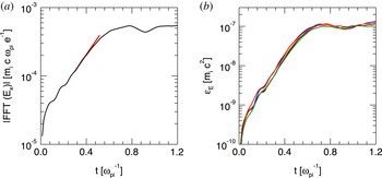
(a) Evolution of the electric field component corresponding to
 $k=153\,\unicode[STIX]{x1D714}_{pi}/c$
(black). The over-plotted red line represents the theoretical growth rate as provided by the solution of (4.4). (b) Evolution of the electric field energy for
 $\unicode[STIX]{x0394}x\simeq 1$
(black), 2 (blue), 3.5 (orange), 7 (red) and 14 (green)
 $\unicode[STIX]{x1D706}_{Dc}$
.

Code results have been compared with the numerical solution of (4.4). In this case the domain was discretised with 1024 cells, so that
 $\unicode[STIX]{x0394}x=3.3\times 10^{-4}\,c/\unicode[STIX]{x1D714}_{pi}\simeq \unicode[STIX]{x1D706}_{Dc}$
, with
 $\unicode[STIX]{x1D706}_{Dc}$
the smallest spatial scale in the system. The time step was chosen to be the maximum time step allowed in an explicit code:
 $\unicode[STIX]{x0394}t\simeq \unicode[STIX]{x0394}x/c=3.2\times 10^{-4}\,\unicode[STIX]{x1D714}_{pi}^{-1}$
. Figure 4(a) shows the growth rate
 $\unicode[STIX]{x1D6E4}$
of the field component corresponding to
 $k=153\,\unicode[STIX]{x1D714}_{pi}/c$
. The simulation growth rate is measured to be
 $\unicode[STIX]{x1D6E4}=5.6\,\unicode[STIX]{x1D714}_{pi}$
, as predicted by the theory.
A set of simulations have been carried out to check the code convergence and stability versus coarser spatial discretization. Results are reported in figure 4(b), which shows the evolution of the electric field energy for
 $\unicode[STIX]{x0394}x=3.3\times 10^{-4}/5.2\times 10^{-3}\,c/\unicode[STIX]{x1D714}_{pi}\simeq 1/15\,\unicode[STIX]{x1D706}_{Dc}$
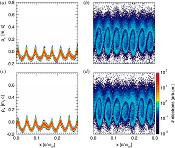
. In all the cases analysed, the field energy shows the same trend. The correct growth rate of the instability can be retrieved by all the simulations and the same saturation level is reached. The particle phase spaces have been also compared, to determine whether kinetic effects were properly retained. Figure 5 shows the longitudinal phase space for cold and hot electrons at the saturation of the instability (
 $t=0.7\,\unicode[STIX]{x1D714}_{pi}^{-1}$
), obtained with the finest and the coarsest resolutions. Plots do not show appreciable differences: particle trapping is well described even when
 $\unicode[STIX]{x0394}x\gg \unicode[STIX]{x1D706}_{Dc}$
, confirming that the results are accurate and the algorithm can reproduce well the physics with a coarse discretization.
Cold (a,c) and hot (b,d) electron phase space at the saturation of the instability (
 $t=0.7\,\unicode[STIX]{x1D714}_{pi}^{-1}$
). Results (a) and (b) have been obtained with
 $\unicode[STIX]{x0394}x\simeq \unicode[STIX]{x1D706}_{Dc}$
, while (c) and (d) with
 $\unicode[STIX]{x0394}x\simeq 7\,\unicode[STIX]{x1D706}_{Dc}$
.

4.3 Reconnection example
Magnetic reconnection (Biskamp Reference Biskamp2000) is an important example of electromagnetic processes with multiple scales. During reconnection, electrons and ions become separated from the field lines, braking the frozen-in condition. Magnetic energy is released to particle energy (macroscopic flows and heating). The critical aspect of interest here is that the reconnection process presents two scales: the ions become decoupled from the frozen-in flow on a scale comparable with the ion inertial length,
 $d_{i}=c/\unicode[STIX]{x1D714}_{pi}$
, the electrons instead decouple on a much smaller scale, the electron skin depth,
 $d_{e}=c/\unicode[STIX]{x1D714}_{pe}$
(Birn & Priest Reference Birn and Priest2007). The Debye length does not play a significant role in this specific process, although it does play a role in other aspects, especially along the separatrices (Lapenta et al.
Reference Lapenta, Markidis, Divin, Goldman and Newman2010, Reference Lapenta, Markidis, Divin, Goldman and Newman2011; Divin et al.
Reference Divin, Lapenta, Markidis, Newman and Goldman2012; Lapenta et al.
Reference Lapenta, Markidis, Divin, Newman and Goldman2014). For very cold plasmas the ratio of
 $d_{e}/\unicode[STIX]{x1D706}_{De}$
can be very large. Explicit, but even previous semi-implicit methods, are limited in how far they can exceed the condition
 $\unicode[STIX]{x0394}x/\unicode[STIX]{x1D706}_{De}<\unicode[STIX]{x03C0}$
. We show here one example, based on the classic GEM challenge (Birn et al.
Reference Birn, Drake, Shay, Rogers, Denton, Hesse, Kuznetsova, Ma, Bhattacharjee and Otto2001).
The system is periodic in all directions and the initial state corresponds to a double Harris equilibrium. In particular the initial magnetic field in the
 $x$
-direction is given by (Drake et al.
Reference Drake, Shay, Thongthai and Swisdak2005):
 $$\begin{eqnarray}B_{x}(y)=B_{0}\left(-1+\tanh \left(\frac{y-y_{B}}{\unicode[STIX]{x1D6FF}}\right)+\tanh \left(\frac{y_{T}-y}{\unicode[STIX]{x1D6FF}}\right)\right),\end{eqnarray}$$
where
 $L_{x}$
and
 $L_{y}$
are the dimensions of the box,
 $y_{B}=0.25\,L_{y}$
and
 $y_{T}=0.75\,L_{y}$
the position of the two current sheets. The magnetic field
 $B_{0}$
is computed from the pressure balance condition
 $n_{0}(T_{e}+T_{i})=B_{0}^{2}/8\unicode[STIX]{x03C0}$
,
 $T_{e}$
and
 $T_{i}$
being the temperature of the electrons and ions. The magnetic field in
 $z$
and
 $y$
directions is zero as are all the components of the electric field. All the particles of the same species are at the same thermal temperature with a Maxwellian distribution and the drift velocity is set to ensure force balance.
To trigger the non-stationary reconnection we add a perturbation to the initial magnetic field. The perturbation chosen in this case is the same as in Lapenta et al. (Reference Lapenta, Markidis, Divin, Goldman and Newman2010) and its vector potential is given by
 $$\begin{eqnarray}\displaystyle \unicode[STIX]{x1D6FF}\boldsymbol{A}(x,y) & = & \displaystyle A_{0}\cos (2\unicode[STIX]{x03C0}(x-x_{T})/\unicode[STIX]{x1D6FF})\cos (\unicode[STIX]{x03C0}(y-y_{T})/\unicode[STIX]{x1D6FF})\text{e}^{-((x-x_{T})^{2}+(y-y_{T})^{2})/\unicode[STIX]{x1D6FF}}\nonumber\\ \displaystyle & & \displaystyle +\,A_{0}\cos (2\unicode[STIX]{x03C0}(x-x_{B})/\unicode[STIX]{x1D6FF})\cos (\unicode[STIX]{x03C0}(y-y_{B})/\unicode[STIX]{x1D6FF})\text{e}^{-((x-x_{B})^{2}+(y-y_{B})^{2})/\unicode[STIX]{x1D6FF}},\end{eqnarray}$$
where
 $x_{B}=0.25\,L_{x}$
and
 $x_{T}=0.75\,L_{x}$
. The initial charge density of the system is given by (4.8)
 $$\begin{eqnarray}\unicode[STIX]{x1D70C}(y)=n_{0}(\text{sech}^{2}(y-y_{T})+\text{sech}^{2}(y-y_{B}))+n_{\infty },\end{eqnarray}$$
where
 $n_{0}$
is the density of particles with drift velocity and
 $n_{\infty }$
is the density of the background particles (particles without drift velocity). This perturbation is similar to that in the standard GEM challenge (Birn et al.
Reference Birn, Drake, Shay, Rogers, Denton, Hesse, Kuznetsova, Ma, Bhattacharjee and Otto2001), but more localized in space as in Lapenta et al. (Reference Lapenta, Markidis, Divin, Goldman and Newman2010). The perturbation is strong, bringing reconnection immediately to a nonlinear state, avoiding the need for a long linear phase of slow growth. This is the central feature of the GEM challenge that makes it a widely used benchmark for new codes.
We have carried out two sets of simulations, in both we use
 $m_{i}/m_{e}=25$
,
 $T_{i}/T_{e}=5$
,
 $n_{0}/n_{\infty }=1$
,
 $\unicode[STIX]{x1D6FF}=0.5$
,
 $L_{x}=25\,c/\unicode[STIX]{x1D714}_{pi}$
and
 $L_{y}=12.5\,c/\unicode[STIX]{x1D714}_{pi}$
. The number of cells in each direction are
 $256\times 128\times 1$
. In the case of high temperature the thermal velocity of the electrons is
 $v_{th,e}=0.1\,c$
which leads to
 $B_{0}=0.0693\,m_{i}c\unicode[STIX]{x1D714}_{pi}/e$
and in the case of low temperature
 $v_{th,e}=0.001\,c$
with
 $B_{0}=000693\,m_{i}c\unicode[STIX]{x1D714}_{pi}/e$
.
For the high temperature case we use two values of the time step
 $\unicode[STIX]{x0394}t=0.1\,\unicode[STIX]{x1D714}_{pi}^{-1}$
and
 $\unicode[STIX]{x0394}t=0.4\,\unicode[STIX]{x1D714}_{pi}^{-1}$
. In the simulations performed with iPic3D the damping parameter used is
 $\unicode[STIX]{x1D703}=1$
, otherwise the energy dramatically increases and the code crashes. With ECsim we use
 $\unicode[STIX]{x1D703}=0.5$
(in which case the energy is exactly conserved) and
 $\unicode[STIX]{x1D703}=1$
, which damps out the high frequencies and hence prevents energy conservation. It is important to note that conversely to what happens in iPic3D, when the energy is not conserved in ECsim, it is because some frequencies are damped, which means that the energy associated with them is lost. Therefore, the energy will always decrease and the system is stable.
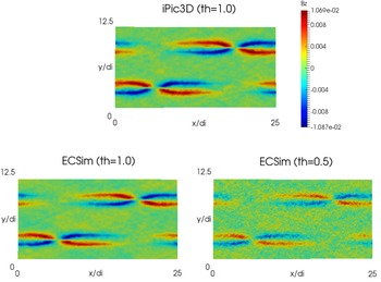
High temperature. Cases with
 $\unicode[STIX]{x0394}t=0.4\,\unicode[STIX]{x1D714}_{pi}^{-1}$
, out of plane magnetic field (
 $B_{z}$
) at
 $t=240\,\unicode[STIX]{x1D714}_{pi}^{-1}$
. In the top panel, the result from iPic3D with
 $\unicode[STIX]{x1D703}=1.0$
; in the bottom panel, from ECsim with
 $\unicode[STIX]{x1D703}=1.0$
(left) and
 $\unicode[STIX]{x1D703}=0.5$
(right)

In figure 6 we see the magnetic field out of plane (
 $z$
-component) from three different simulations, iPic3D (
 $\unicode[STIX]{x1D703}=1$
), ECsim with
 $\unicode[STIX]{x1D703}=1$
and ECsim with
 $\unicode[STIX]{x1D703}=0.5$
. All the results are in good agreement and the only difference is that in the case with
 $\unicode[STIX]{x1D703}=0.5$
there is more noise, which is due to the high frequencies damped in the other cases.
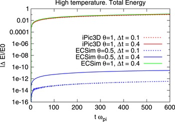
High temperature. Absolute value of the variation of the total energy (in logarithmic scale) for different values of the time step.

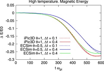
High temperature. Variation of the magnetic energy for different values of the time step.

In figure 7 the variation of the total energy is shown and, as we expected, the total energy is conserved up to the tolerance of the field solver (in all cases
 $10^{-12}$
) in the results from ECsim with
 $\unicode[STIX]{x1D703}=0.5$
. The evolution of the magnetic energy (figure 8), which gives us an idea of the reconnection rate, is very similar in all cases.
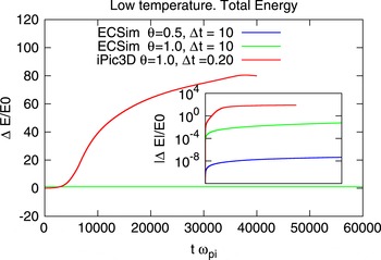
Low temperature. Variation of the total energy in linear scale and its absolute value in logarithmic scale (inner figure).

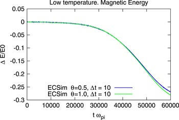
Low temperature. Variation of the magnetic energy.

The situation in the low temperature case is completely different. If in the high temperature case we needed to simulate up to
 $t\approx 600\,\unicode[STIX]{x1D714}_{pi}^{-1}$
, here we will need
 $t\approx 60\,000\,\unicode[STIX]{x1D714}_{pi}^{-1}$
. If we use the same time step the simulation would be 100 times more expensive, and even in that case, iPic3D is not capable of dealing with this situation: after a given number of cycles the energy dramatically increases (see figure 9) and the simulation has no physical meaning. On the other hand, in ECsim the energy is exactly conserved and hence we are able to use a larger time step without any problems. But even with
 $\unicode[STIX]{x1D703}=1$
(which no longer guarantees energy conservation), the energy remains stable, it changes, but the variation is small enough to not distort the results. This can be seen in figure 10 where the variation of the magnetic energy from ECsim with
 $\unicode[STIX]{x1D703}=1$
and
 $\unicode[STIX]{x1D703}=0.5$
is shown.
The new method can capture the kinetic level of description for both species. While some aspects of reconnection can be captured accurately by fluid models (see Birn & Priest (Reference Birn and Priest2007) for a review), to obtain the phase space distribution of electron and ions, a full kinetic description is needed. As reconnection develops, the average electron flows determine the electric and magnetic field structure. The most typical feature is the formation of the Hall magnetic field, seen in figure 6. These effects can be captured also by fluid models, but the results reported in figures 11 and 12 are typical of kinetic approaches.
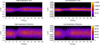
Electron and ion longitudinal phase space (
 $v_{x}$
versus
 $x$
). Only particles located in the band
 $3.0d_{i}<y<3.1d_{i}$
are considered. Colours are proportional to the charge density. The scale of the ion charge density is shown on the right top side and the one of the electrons on the right bottom part.

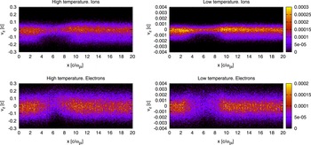
Electron and ion transversal phase space (
 $v_{z}$
versus
 $x$
). Only particles located in the band
 $3.0d_{i}<y<3.1d_{i}$
are considered. Colours are proportional to the charge density. The scale of the ion charge density is shown on the right top side and the one of the electrons on the right bottom part.

In figure 11, the electron and ion phase space is reported in the cross-section
 $(x,v_{x})$
. The four panels compare ions and electrons and the cold and hot cases (note the different velocity axis). Ions are accelerated at the reconnection site (located near
 $x/d_{i}=6$
). We are showing here the distribution function for particles located in the range
 $y/d_{i}=[3,3.1]$
and are integrated in the two velocities not reported. Figure 12 reports the distribution function for the same
 $y$
range but in the plane
 $(x,v_{z})$
(integrated in the other two velocities).
For the distribution in
 $v_{x}$
, at each
 $x$
the distribution is fairly Maxwellian, as can be observed by its symmetry with respect with the peak. This effect is due to the nature of the particle acceleration along
 $x$
that is caused by the Lorentz force associated with the vertical magnetic field (Goldman et al.
Reference Goldman, Lapenta, Newman, Markidis and Che2011). Instead, the distribution changes strongly in space, being much narrower at the reconnection site and broadening away from it.
The distribution in
 $v_{z}$
, is highly non-Maxwellian. The acceleration along the
 $z$
-direction is caused by the reconnection electric field active effectively in the electron diffusion region where the electrons become demagnetized and instead of
 $\boldsymbol{E}\times \boldsymbol{B}$
drifting are accelerated (Moses, Finn & Ling Reference Moses, Finn and Ling1993; Divin et al.
Reference Divin, Markidis, Lapenta, Semenov, Erkaev and Biernat2010). A consequence if this mechanism is the strong distortion of the particle distribution in the vicinity of the
 $x$
-point. Moving away from the
 $x$
-point the distribution remains strongly non-Maxwellian, especially for the ions, with a distinct asymmetry between positive and negative
 $v_{z}$
, the negative side having a much wider width.
In summary, we have shown that, in the situations where iPic3D can be used, the new code gives the same result, and in those set-ups in which iPic3D is limited, the new code is able to give good results, and even more, to speed up the simulation time by using a larger time step. The new method is capable not only of capturing the nonlinear macroscopic effects of reconnection, such as the production of the Hall magnetic field, but also the detailed microphysics of particle acceleration at the kinetic level.
5 Conclusions
We presented the ECsim algorithm and tested its ability to handle multiple scales. The ECsim is based on two innovations. First, a new mover is presented, a hybrid of the
 $\unicode[STIX]{x1D703}$
-scheme and the leap-frog algorithm. The new mover is still implicit and unconditionally stable but it allows us to more readily compute the interpolation between particles and cells. Second, we use a new method to compute the current needed for Maxwell equations. The new method introduces a number of mass matrices that produce an exact representation of the current. The relationship between the electric field and the current mediated by the mass matrix is an exact consequence of the mover without any linearization and it is naturally linear. These two innovations lead to one critical consequence: the new ECsim is exactly energy conserving. This point is important in two aspects. First, energy conservation is a desirable property because energy is of course conserved in reality and missing this aspect, as most PIC method do, is unsatisfactory. Second, the existence of energy conservation is in itself a proof on nonlinear stability in the
 $L_{2}$
-norm. The fact that an energy integral exist to limit the energy error eliminates the tendency of PIC methods to numerically heat.
Compared with explicit PIC (Birdsall & Langdon Reference Birdsall and Langdon2004), the new method eliminates all instabilities and in particular the finite grid instability. This numerical instability leads to numerical exponential growth of the total energy and destroys the simulations when the grid spacing far exceeds the Debye length. In the simplest explicit PIC method, this condition requires
 $\unicode[STIX]{x0394}x/\unicode[STIX]{x1D706}_{De}<\unicode[STIX]{x03C0}$
, a condition that can be somewhat relaxed using higher-order interpolation. The ECsim eliminates this completely, allowing the grid spacing to be several orders of magnitude larger than the Debye length, we reported recently a case where the grid spacing was 16 orders of magnitude larger (Lapenta Reference Lapenta2016).
Compared with fully implicit methods (Chen et al. Reference Chen, Chacón and Barnes2011; Lapenta & Markidis Reference Lapenta and Markidis2011; Markidis & Lapenta Reference Markidis and Lapenta2011) that also conserve energy exactly and are stable for any grid spacing, the ECsim differs in its linear formulation of the field equations that removes the need for the Newton nonlinear iteration.
Compared with previous semi-implicit methods, such as the moment implicit (Brackbill & Forslund Reference Brackbill and Forslund1982; Lapenta, Brackbill & Ricci Reference Lapenta, Brackbill and Ricci2006; Markidis et al.
Reference Markidis and Lapenta2010) and the direct implicit (Langdon et al.
Reference Langdon, Cohen and Friedman1983) methods, ECsim does not require any linearization step. The linearization used in the previous semi-implicit methods breaks energy conservation and
 $L_{2}$
stability, reintroducing the finite grid instability and a limitation to the size of the cells allowed. Practice and experience ensures that in the implicit moment method, the condition
 $\unicode[STIX]{x0394}x<v_{th,e}\unicode[STIX]{x0394}t$
ensures no finite grid instability. This condition allows for much larger cells than in the explicit PIC, but still prevents the method from exceeding the Debye scales by too large a factor. This factor, unfortunately, is empirical and problem dependent. Practice shows that a plasma with low temperature electrons where the skin depth is much larger than the Debye length,
 $d_{e}\gg \unicode[STIX]{x1D706}_{De}$
, is very hard to model without resolving very small scales. ECsim, instead, allows the user to completely ignore this limitation and set the grid spacing entirely on accuracy considerations without worrying about stability.
The results section highlights the advantages in three practical cases. First, the ion acoustic wave shows the ability of ECsim to resolve accurately the ion scales without needing to resolve the electron scales unnecessarily. Second, the electron acoustic instability is used to show how ECsim can resolve one subpopulation of electrons without needing to resolve the smallest scales of the cold electrons. Finally, for a classic reconnection problem, the GEM challenge, ECsim shows the ability described above to resolve the electron scale at the skin depth level without suffering any finite grid instability even for very cold plasmas where
 $d_{e}\gg \unicode[STIX]{x1D706}_{De}$
.
Acknowledgements
The present work is supported by the US Air Force EOARD Project FA2386-14-1-0052, by the Onderzoekfonds KU Leuven (Research Fund KU Leuven, GOA scheme and Space Weaves RUN project) and by the Interuniversity Attraction Poles Programme of the Belgian Science Policy Office (IAP P7/08 CHARM). This research used resources of the National Energy Research Scientific Computing Center, which is supported by the Office of Science of the US Department of Energy under Contract no. DE-AC02-05CH11231. Additional computing has been provided by NASA NAS and NCCS High Performance Computing, by the Flemish Supercomputing Center (VSC) and by PRACE Tier-0 allocations.