



1 Introduction
Oscillatory flows are found in nature and in technological applications, especially in ocean engineering which deals primarily with wave phenomena. In marine renewable energy, this type of flows is important for wave energy extraction devices. Other applications include offshore structures and ships. The Reynolds number (
 $Re$
) of these flows is high, justifying the use of the potential flow approximation for the bulk of the fluid, where viscosity effects are of higher order. However, at small distances from solid boundaries or at fluid–fluid interfaces in the presence of boundary layers, the assumption of inviscid behaviour ceases to be valid. Moreover, when such boundary layers separate and vortex shedding occurs, viscous effects can become non-negligible at larger distances in the interior of the fluid. This is characteristic of wave energy devices operating in extreme conditions with large amplitudes of oscillation, when the effects of boundary layer separation on the performance of the device become significant. As the oscillatory flow evolves, the shed vorticity sheet can be in distinct phases of its evolution and its effect on the forces on the device will vary with time.
For the oscillating wave surge converter (Dias et al.
Reference Dias, Renzi, Gallagher, Sarkar, Wei, Abadie, Cummins and Rafiee2017), viscous effects were previously studied in Wei et al. (Reference Wei, Rafiee, Henry and Dias2015) and others for normal operating conditions. It was found that for small Keulegan–Carpenter (
 $KC$
) numbers, the shed vorticity layer rolls-up into vortices that do not travel far from the body. This shed vorticity layer and its dissipative effects were later modelled in an inviscid setting as a pressure drop across the device’s edges (Cummins & Dias Reference Cummins and Dias2017).
A model for the viscous oscillatory flow near a solid wall is an infinite plate oscillating in its own plane with velocity
 $U_{0}$
in an otherwise quiescent fluid. This set-up is known as Stokes’ second problem (Schlichting & Gersten Reference Schlichting and Gersten2003). The laminar steady case provides one of the few known analytical solutions of the Navier–Stokes equations, characterized by alternating layers of motion that diffuses from the wall into the fluid. The thickness
 $\unicode[STIX]{x1D6FF}$
of the layer where the motion of the wall is diffused is
 $(2\unicode[STIX]{x1D708}/\unicode[STIX]{x1D714})^{1/2}$
, where
 $\unicode[STIX]{x1D708}$
is the kinematic viscosity of the fluid and
 $\unicode[STIX]{x1D714}$
the angular frequency of the oscillations. For prototypical applications of this problem however, the ratio
 $Re_{\unicode[STIX]{x1D6FF}}=U_{0}\unicode[STIX]{x1D6FF}/\unicode[STIX]{x1D708}$
can be
 $\gg 1$
, invalidating the laminar model of the Stokes boundary layer.
The Stokes boundary layer can exhibit distinct regimes, depending on the value of
 $Re_{\unicode[STIX]{x1D6FF}}$
: laminar; disturbed laminar; intermittently turbulent (IT); fully turbulent (FT). The laminar regime can be observed for
 $Re_{\unicode[STIX]{x1D6FF}}$
up to 257 (Jensen, Sumer & Fredsøe Reference Jensen, Sumer and Fredsøe1989) and the flow consists of the classical solution by Stokes where layers of fluid
 $2\unicode[STIX]{x03C0}/\unicode[STIX]{x1D6FF}$
apart oscillate in phase (Schlichting & Gersten Reference Schlichting and Gersten2003).
In the disturbed laminar regime, from
 $Re_{\unicode[STIX]{x1D6FF}}\sim 100$
up to a critical value of approximately 550 (Hino et al.
Reference Hino, Kashiwayanagi, Nakayama and Hara1983), depending on the dimensions of the channel or pipe, disturbances appear superimposed on the base laminar flow, initially small, they grow at the end of the decelerating stage and reach considerable magnitude at the beginning of the accelerating stage of the cycle (Vittori & Verzicco Reference Vittori and Verzicco1998).
The intermittently turbulent regime has been detected experimentally for
 $Re_{\unicode[STIX]{x1D6FF}}\geqslant$
385 (Jensen et al.
Reference Jensen, Sumer and Fredsøe1989) and is characterized by turbulent bursts in the decelerating stage and by relaminarization of the flow in the accelerating stage (Hino, Sawamoto & Takasu Reference Hino, Sawamoto and Takasu1976; Eckmann & Grotberg Reference Eckmann and Grotberg1991). The fully turbulent regime has been recorded throughout the cycle for
 $Re_{\unicode[STIX]{x1D6FF}}=3460$
(Jensen et al.
Reference Jensen, Sumer and Fredsøe1989).
Concerning the stability of the Stokes boundary layer, Von Kerczek & Davis (Reference Von Kerczek and Davis1974) showed that it is absolutely stable for infinitesimal perturbations for
 $Re_{\unicode[STIX]{x1D6FF}}$
up to 800 and proposed that it may be stable for all
 $Re_{\unicode[STIX]{x1D6FF}}$
for that type of perturbations. Transition may nonetheless be explained by a secondary instability mechanism of two-dimensional (2-D) finite amplitude waves to 3-D infinitesimal perturbations (Akhavan, Kamm & Shapiro Reference Akhavan, Kamm and Shapiro1991b
) or by wall imperfections (Vittori & Verzicco Reference Vittori and Verzicco1998). After the inception of turbulence in the IT regime, during the accelerating stage, turbulence is initiated by shear instabilities located not far from the wall but these are suppressed and unable to develop. When the flow begins to accelerate, turbulence grows explosively and is maintained by the bursting type of motion (Hino et al.
Reference Hino, Kashiwayanagi, Nakayama and Hara1983).
A well-known aspect of canonical turbulent boundary layers is the existence of coherent structures, i.e. spatio-temporal patterns that repeatedly appear in the flow, giving turbulence a degree of deterministic organization, in the sense of a correlated and concentrated dynamic quality. Vorticity has been most extensively used (Jeong & Hussain Reference Jeong and Hussain1995; Jeong et al. Reference Jeong, Hussain, Schoppa and Kim1997), but any flow quantity that exhibits this correlation, including Lagrangian quantities, can be used to identify coherent structures in turbulent boundary layers (Robinson Reference Robinson1991; Green, Rowley & Haller Reference Green, Rowley and Haller2007; Bettencourt, Lopez & Hernandez-Garcia Reference Bettencourt, Lopez and Hernandez-Garcia2013).
It is well known that coherent structures determine mixing, heat transfer and other phenomena in turbulent boundary layers. In the Stokes layer, however, the role played by coherent structures is less clear. The transitional and turbulent states are populated by vortical motions that appear most intensely in the final stages of the deceleration stages. At
 $Re_{\unicode[STIX]{x1D6FF}}\sim 400$
, low-speed streaks emerge at the end of this stage, while the flow reversal causes the destruction of coherent structures (Sarpkaya Reference Sarpkaya1993). In numerical simulations of a pulsating turbulent channel flow, Scotti & Piomelli (Reference Scotti and Piomelli2001) observed the appearance of long and smooth streaks during the acceleration stage that eventually transition into turbulence and break up in later stages of the cycle. The
 $Q$
-criterion (Dubief & Delcayre Reference Dubief and Delcayre2000) showed greater organization during the late turbulent stage of the cycle.
The number of coherent structures present in the turbulent boundary layer is a function of the Reynolds number and also the level of residual turbulence in the acceleration stage. At
 $Re_{\unicode[STIX]{x1D6FF}}=800$
, streamwise streaks appear at the end of the acceleration stage and are present during the deceleration stage (Costamagna, Vittori & Blondeaux Reference Costamagna, Vittori and Blondeaux2003). At
 $Re_{\unicode[STIX]{x1D6FF}}=1790$
, Salon, Armenio & Crise (Reference Salon, Armenio and Crise2007) observed the same sequence of events, but with a half-cycle phase deviation to earlier stages of the cycle, a fact attributed to the different Reynolds number.
Although there are similarities between the canonical turbulent boundary layer and the Stokes boundary layer, in the latter the sequence of events that generate turbulence does not occur randomly but with a time scale of
 $T$
/2, where
 $T$
is the period of the oscillation. In these turbulent states, the flow does not exhibit a sufficient number of symmetric hairpin vortices to generate the low-speed streaks as in the canonical case (Sarpkaya Reference Sarpkaya1993) and no evidence was found of vortices spawning from parent vortical structures. A more recent result is the appearance of turbulent spots in the Stokes boundary layer (Carstensen, Sumer & Fredsøe Reference Carstensen, Sumer and Fredsøe2010; Mazzuoli, Vittori & Blondeaux Reference Mazzuoli, Vittori and Blondeaux2011).
The purpose of this paper is to study the connection between wall pressure fluctuations, wall vorticity and coherent structures in the Stokes boundary layer (for the canonical boundary layer case see Andreopoulos & Agui (Reference Andreopoulos and Agui1996) and references therein), and to attempt to identify the major features of wall pressure and vorticity distributions in the intermittently turbulent regime of the Stokes boundary layer.
In the next section we recall the connection between wall pressure, viscosity and wall vorticity. Section 3 describes the set-up of the direct numerical simulations (DNS). The results are presented and discussed in § 4. Conclusions are drawn in § 5.
2 Boundary vorticity flux
The central role played by vorticity
 $\unicode[STIX]{x1D734}=\unicode[STIX]{x1D735}\times \boldsymbol{u}$
in fluid motions results from the fact that it is a measure of the transverse shearing process, one of the two dynamical processes in the flow of a viscous fluid, the other being the compressive process. To see this, we recall Cauchy’s equation for the mechanical equilibrium of a material element of a continuum with density
 $\unicode[STIX]{x1D70C}$
:
 $$\begin{eqnarray}\frac{\text{D}\boldsymbol{u}}{\text{D}t}=\boldsymbol{a}=\boldsymbol{f}+\frac{1}{\unicode[STIX]{x1D70C}}(\unicode[STIX]{x1D735}\boldsymbol{\cdot }\unicode[STIX]{x1D64F}),\end{eqnarray}$$
where
 $\boldsymbol{a}$
is the acceleration,
 $\boldsymbol{f}$
is the body force,
 $\unicode[STIX]{x1D64F}$
is the stress tensor and its divergence the surface force vector, whose Stokes–Helmholtz decomposition gives
 $$\begin{eqnarray}\unicode[STIX]{x1D735}\boldsymbol{\cdot }\unicode[STIX]{x1D64F}=-\unicode[STIX]{x1D735}\unicode[STIX]{x1D719}+\unicode[STIX]{x1D735}\times \boldsymbol{A},\quad \unicode[STIX]{x1D735}\boldsymbol{\cdot }\boldsymbol{A}=0.\end{eqnarray}$$
In (2.2), the scalar and vector potentials
 $\unicode[STIX]{x1D719}$
and
 $\boldsymbol{A}$
represent the compressing/expanding process and the shearing process, respectively. The role of vorticity can be made clear if we consider (2.2) for a Newtonian fluid with constant viscosity
 $\unicode[STIX]{x1D707}$
:
 $$\begin{eqnarray}\unicode[STIX]{x1D735}\boldsymbol{\cdot }\unicode[STIX]{x1D64F}=-\unicode[STIX]{x1D735}\unicode[STIX]{x1D6F1}-\unicode[STIX]{x1D707}\unicode[STIX]{x1D735}\times \unicode[STIX]{x1D734}.\end{eqnarray}$$
Vorticity then plays the role of the shear variable
 $\boldsymbol{A}$
, while
 $\unicode[STIX]{x1D6F1}=p$
under the assumption of incompressibility. For a more general form of (2.3) and a discussion of the coupling between the two processes, the reader is referred to Wu & Wu (Reference Wu and Wu1996).
In a Lagrangian frame of reference, the rate of change of the vorticity of an infinitesimal fluid particle is found by taking the curl of (2.1) and using the continuity equation:
 $$\begin{eqnarray}\frac{\text{D}\unicode[STIX]{x1D734}}{\text{D}t}=\unicode[STIX]{x1D734}\boldsymbol{\cdot }\unicode[STIX]{x1D735}\boldsymbol{u}+\unicode[STIX]{x1D735}\times \boldsymbol{f}-\unicode[STIX]{x1D735}\times (\unicode[STIX]{x1D708}\unicode[STIX]{x1D735}\times \unicode[STIX]{x1D734}),\end{eqnarray}$$
where
 $\unicode[STIX]{x1D708}=\unicode[STIX]{x1D707}/\unicode[STIX]{x1D70C}$
is the kinematic viscosity. Since the curl of (2.1) is the specific torque of the fluid particle, the total specific torque of the fluid is given by
 $$\begin{eqnarray}\frac{\text{D}}{\text{D}t}\int _{{\mathcal{V}}}\unicode[STIX]{x1D734}\,\text{d}V=\int _{{\mathcal{V}}}\unicode[STIX]{x1D734}\boldsymbol{\cdot }\unicode[STIX]{x1D735}\boldsymbol{u}\,\text{d}V+\int _{{\mathcal{V}}}\unicode[STIX]{x1D735}\times \boldsymbol{f}\,\text{d}V-\unicode[STIX]{x1D708}\int _{{\mathcal{D}}}\boldsymbol{n}\times (\unicode[STIX]{x1D735}\times \unicode[STIX]{x1D734})\,\text{d}S.\end{eqnarray}$$
Here, the total torque has contributions from vortex stretching, non-conservative body forces and a third term that contains the contributions of the boundary
 ${\mathcal{D}}$
(Wu & Wu Reference Wu and Wu1996), whose outward normal is
 $\boldsymbol{n}$
. According to (2.5) any boundary that exerts a torque on the neighbouring fluid will change its vorticity and this change occurs through the mediation of viscosity, as a flux of vorticity into the fluid from the boundary. This relationship was first recognized by Lighthill (Reference Lighthill and Rosenhead1963) when introducing the concept of boundary vorticity flux from a two-dimensional solid wall due to the no-slip boundary condition. The boundary vorticity flux
 $\unicode[STIX]{x1D70E}$
was defined then as the normal gradient of vorticity at the wall:
 $$\begin{eqnarray}\unicode[STIX]{x1D70E}=\unicode[STIX]{x1D708}\frac{\unicode[STIX]{x2202}\unicode[STIX]{x1D6FA}}{\unicode[STIX]{x2202}n}.\end{eqnarray}$$
The strong coupling between
 $\unicode[STIX]{x1D748}$
, the vorticity source strength and the processes occurring in the interior of the fluid becomes clear when the tangential component of the momentum balance equations is written at the wall (here located along the
 $x$
-axis):
 $$\begin{eqnarray}\unicode[STIX]{x1D708}\frac{\unicode[STIX]{x2202}\unicode[STIX]{x1D6FA}}{\unicode[STIX]{x2202}n}=-\frac{1}{\unicode[STIX]{x1D70C}}\frac{\unicode[STIX]{x2202}p}{\unicode[STIX]{x2202}x}.\end{eqnarray}$$
This coupling mechanism was depicted in Lighthill (Reference Lighthill and Rosenhead1963) by an irrotational small fluid sphere located at the wall that acquires vorticity by the action of a pressure gradient. The pressure gradient is parallel to the boundary, forcing the fluid sphere to roll along the wall due to the no-slip condition.
The boundary vorticity flux
 $\unicode[STIX]{x1D748}$
produced by a three-dimensional solid stationary wall
 ${\mathcal{W}}$
where the no-slip condition is enforced, that is
 $\boldsymbol{u}_{0}=0$
is of special interest. (The subscript 0 refers to quantities evaluated at the wall.)
The mechanisms that create vorticity at the wall are pressure gradient, wall acceleration and viscous stresses (with wall normal and tangential components) (Wu & Wu Reference Wu and Wu1996):
 $$\begin{eqnarray}\displaystyle & \displaystyle \unicode[STIX]{x1D748}_{p}=\boldsymbol{n}\times \unicode[STIX]{x1D735}(p_{0}/\unicode[STIX]{x1D70C}), & \displaystyle\end{eqnarray}$$
 $$\begin{eqnarray}\displaystyle & \displaystyle \unicode[STIX]{x1D748}_{a}=\boldsymbol{n}\times \boldsymbol{a}_{0}, & \displaystyle\end{eqnarray}$$
 $$\begin{eqnarray}\displaystyle & \displaystyle \unicode[STIX]{x1D748}_{\unicode[STIX]{x03C0}}=-(\boldsymbol{n}\times \unicode[STIX]{x1D749}_{0})\boldsymbol{\cdot }\boldsymbol{K}, & \displaystyle\end{eqnarray}$$
 $$\begin{eqnarray}\displaystyle & \displaystyle \unicode[STIX]{x1D748}_{n}=-\boldsymbol{n}\{\boldsymbol{n}\boldsymbol{\cdot }(\unicode[STIX]{x1D735}\times \unicode[STIX]{x1D749}_{0})\}. & \displaystyle\end{eqnarray}$$
In (2.8a
) the gravitational effect is discarded. The two inviscid components
 $\unicode[STIX]{x1D748}_{p}$
and
 $\unicode[STIX]{x1D748}_{a}$
produce vorticity tangent to the wall. In (2.8c
) and (2.8d
) the contributions of viscosity to the boundary vorticity appear as a tangential component due to wall curvature
 $\boldsymbol{K}$
and skin friction
 $\unicode[STIX]{x1D749}_{0}$
and a normal component due to a rotational skin friction distribution. At large
 $Re$
, the inviscid components are much larger than the viscous components. It is worth noting that while there are components of the boundary vorticity flux that are independent of the fluid viscosity, the vorticity flux at a solid wall is a product of the fluid viscosity through the no-slip condition.
The pressure component is perhaps the most basic source of vorticity creation at a solid wall and was the first to be explained (Lighthill Reference Lighthill and Rosenhead1963). It is also the only source in a two-dimensional, stationary wall. The wall acceleration component (2.8b
) will vanish if the acceleration is normal to the wall orientation. Regarding the viscous components, they can only be present in three-dimensional cases. The tangential component exists in the presence of wall curvature while the normal component is related to the configuration of the
 $\unicode[STIX]{x1D749}_{0}$
field. While for large
 $Re$
, the viscous components are much smaller than their inviscid counterparts, the normal viscous component can attain large values near separation lines and in the inner wall region of turbulent boundary layers (Wu & Wu Reference Wu and Wu1996).
In turbulent flows, Andreopoulos & Agui (Reference Andreopoulos and Agui1996) measured strong fluctuations of
 $\unicode[STIX]{x1D70E}_{p}$
in a zero pressure gradient two-dimensional boundary layer. The boundary vorticity flux showed very strong fluctuations associated with small-scale turbulent structures. Uncorrelated pressure signals were responsible for the major contributions to the turbulent vorticity fluxes. Furthermore, Andreopoulos & Agui (Reference Andreopoulos and Agui1996) indicated that these uncorrelated pressure signals contain an extended range of eddy sizes, allowing for an influence of large-scale vortex structures in the near-wall vorticity production.
Domain of the direct numerical simulation of the Stokes boundary layer. Flow directions are named as follows: streamwise is
 $x_{1}$
; cross-stream is
 $x_{2}$
; spanwise is
 $x_{3}$
; the no-slip wall is located at
 $x_{2}=0$
(light grey surface). Oscillatory mean flow is in the longitudinal direction.

Two-point auto-correlations of the velocity field for
 $\unicode[STIX]{x1D719}=170^{\circ }$
at
 $x_{2}/\unicode[STIX]{x1D6FF}=0.5$
. (a) Streamwise; (b) spanwise: streamwise velocity (solid); spanwise velocity (dashed); wall normal velocity (dash–dotted).
 $r$
is the spatial lag.

3 DNS set-up
The direct numerical simulations of the Stokes boundary layer were set-up in a rectangular box with dimensions
 $(L_{1},L_{2},L_{3})=(16\unicode[STIX]{x03C0}\unicode[STIX]{x1D6FF},8\unicode[STIX]{x03C0}\unicode[STIX]{x1D6FF},8\unicode[STIX]{x03C0}\unicode[STIX]{x1D6FF})$
. Here
 $x_{1}$
is the streamwise direction, along which the oscillating free-stream motion is imposed,
 $x_{2}$
is the cross-stream direction (
 $x_{2}=0$
is the no-slip solid boundary) and
 $x_{3}$
is the spanwise direction that forms a right handed coordinate system with
 $x_{1}$
and
 $x_{2}$
(see figure 1).
The domain was discretized in
 $(n_{1},n_{2},n_{3})=(64,96,64)$
cells. The cell size distribution is regular in the streamwise and spanwise directions and stretched in the cross-stream direction according to the following law that gives the
 $x_{2}$
value of the centre of cell
 $j$
:
 $$\begin{eqnarray}x_{2}(j)=\frac{1-r^{j}}{1-r^{n_{2}}}L_{2},\end{eqnarray}$$
where
 $r=((\unicode[STIX]{x0394}x_{2}(n_{2}))/(\unicode[STIX]{x0394}x_{2}(1)))^{1/(1-n_{2})}$
is the expansion ratio. The dimensions of the domain and the number of discrete elements correspond to those of the coarse DNS of Salon et al. (Reference Salon, Armenio and Crise2007). The main requirements on the domain size and numerical grid are (i) that the domain is large enough to hold the largest energy containing eddies and (ii) that the near-wall spacing is fine enough to resolve the turbulent structures that occur in that region.
Grid convergence check. (a) Average wall shear stress in the first half-cycle of the Stokes boundary layer. Averaged over 5 cycles; (b) mean streamwise velocity in wall units at
 $\unicode[STIX]{x1D719}=129^{\circ }$
. Lines as in (a). Circles: experimental data from Jensen et al. (Reference Jensen, Sumer and Fredsøe1989) Test 6 with
 $Re=990$
.

The direct numerical simulation of the Stokes boundary layer was carried out using a finite-volume implementation. The governing equations are the mass and momentum conservation equations:
 $$\begin{eqnarray}\displaystyle & \displaystyle \unicode[STIX]{x1D735}\boldsymbol{\cdot }\boldsymbol{u}=0, & \displaystyle\end{eqnarray}$$
 $$\begin{eqnarray}\displaystyle & \displaystyle \frac{\unicode[STIX]{x2202}\boldsymbol{u}}{\unicode[STIX]{x2202}t}+\unicode[STIX]{x1D735}\boldsymbol{\cdot }(\boldsymbol{u}\boldsymbol{u})-\unicode[STIX]{x1D735}\boldsymbol{\cdot }\unicode[STIX]{x1D708}\unicode[STIX]{x1D735}\boldsymbol{u}=-\frac{1}{\unicode[STIX]{x1D70C}}\unicode[STIX]{x1D735}p+U_{m}\unicode[STIX]{x1D714}\cos (\unicode[STIX]{x1D714}t)\boldsymbol{i}_{\mathbf{1}}. & \displaystyle\end{eqnarray}$$
The momentum source in (3.3) produces an oscillatory flow in the streamwise direction given by
 $U_{m}\sin (\unicode[STIX]{x1D714}t)$
that drives the Stokes boundary layer. The parameters
 $U_{m}$
,
 $\unicode[STIX]{x1D714}$
and
 $\unicode[STIX]{x1D708}$
are chosen to give
 $Re_{\unicode[STIX]{x1D6FF}}=1000$
.
At
 $x_{2}=0$
a no slip condition is imposed on the velocity and at
 $x_{2}=L_{2}$
the boundary is defined as free-slip wall. Periodicity is defined at the vertical boundaries.
The numerical method stores the primitives variables
 $p$
and
 $\boldsymbol{u}$
at the centres of the control volumes. To compute fluxes across control volume faces, the primitive variables are interpolated with a cubic formula to centres of the control volume faces. Spatial derivatives are approximated by standard second-order centred finite differences and the time advancement uses the Crank–Nicolson method. The pressure-implicit with splitting of operators (PISO) algorithm (Issa Reference Issa1986) is used to solve the pressure–velocity coupling.
Time series of velocity components at
 $(x_{1},x_{2},x_{3})=(0.025132,0.0005,0.012566)$
during three cycles of oscillations. (a) streamwise component
 $u_{1}$
; (b) cross-stream component
 $u_{2}$
; (c) spanwise component
 $u_{3}$
.

Time series of (a) volume averaged turbulent kinetic energy and (b) wall friction. Dotted line shows the mean velocity cycle.

Profile of the averaged longitudinal velocity
 $\langle u\rangle$
in inner variables, for several phase angles. Full line: DNS; circles: experimental data from Jensen et al. (Reference Jensen, Sumer and Fredsøe1989) Test 6 with
 $Re=990$
. (a)
 $11^{\circ }$
; (b)
 $28^{\circ }$
; (c)
 $45^{\circ }$
; (d)
 $62^{\circ }$
; (e)
 $96^{\circ }$
; (f)
 $113^{\circ }$
; (g)
 $129^{\circ }$
; (h)
 $146^{\circ }$
.

Profile of longitudinal velocity fluctuations root-mean-sqaure (r.m.s.)
 $(u_{1}^{\prime })_{rms}/U_{0}$
, for several phase angles. Full line: DNS; circles: experimental data from Jensen et al. (Reference Jensen, Sumer and Fredsøe1989) Test 6 with
 $Re=990$
. (a)
 $5^{\circ }$
; (b)
 $40^{\circ }$
; (c)
 $73^{\circ }$
; (d)
 $107^{\circ }$
; (e)
 $140^{\circ }$
; (f)
 $175^{\circ }$
. Note that first value is taken at
 $x_{2}/\unicode[STIX]{x1D6FF}=9\times 10^{-3}$
.

Profile of wall normal velocity fluctuations r.m.s.
 $(u_{2}^{\prime })_{rms}/U_{0}$
, for several phase angles. Full line: DNS; circles: experimental data from Jensen et al. (Reference Jensen, Sumer and Fredsøe1989) Test 6 with
 $Re=990$
. (a)
 $5^{\circ }$
; (b)
 $40^{\circ }$
; (c)
 $73^{\circ }$
; (d)
 $107^{\circ }$
; (e)
 $140^{\circ }$
; (f)
 $175^{\circ }$
. Note that first value is taken at
 $x_{2}/\unicode[STIX]{x1D6FF}=9\times 10^{-3}$
.

Profile of Reynolds stress
 $(u_{1}^{\prime }u_{2}^{\prime })_{rms}$
, for several phase angles. Full line: DNS; circles: experimental data from Jensen et al. (Reference Jensen, Sumer and Fredsøe1989) Test 6 with
 $Re=990$
. (a)
 $5^{\circ }$
; (b)
 $40^{\circ }$
; (c)
 $73^{\circ }$
; (d)
 $107^{\circ }$
; (e)
 $140^{\circ }$
; (f)
 $175^{\circ }$
. Note that first value is taken at
 $x_{2}/\unicode[STIX]{x1D6FF}=9\times 10^{-3}$
.

Iso-surfaces of
 $\langle Q\rangle$
at
 $\unicode[STIX]{x1D719}=85^{\circ }$
. The threshold is
 $Q_{m}\unicode[STIX]{x1D6FF}^{2}/U_{m}^{2}=8.0\times 10^{-4}$
.

Iso-surfaces of
 $\langle Q\rangle$
at
 $\unicode[STIX]{x1D719}=135^{\circ }$
. The threshold is
 $Q_{m}\unicode[STIX]{x1D6FF}^{2}/U_{m}^{2}=7.4\times 10^{-3}$
.
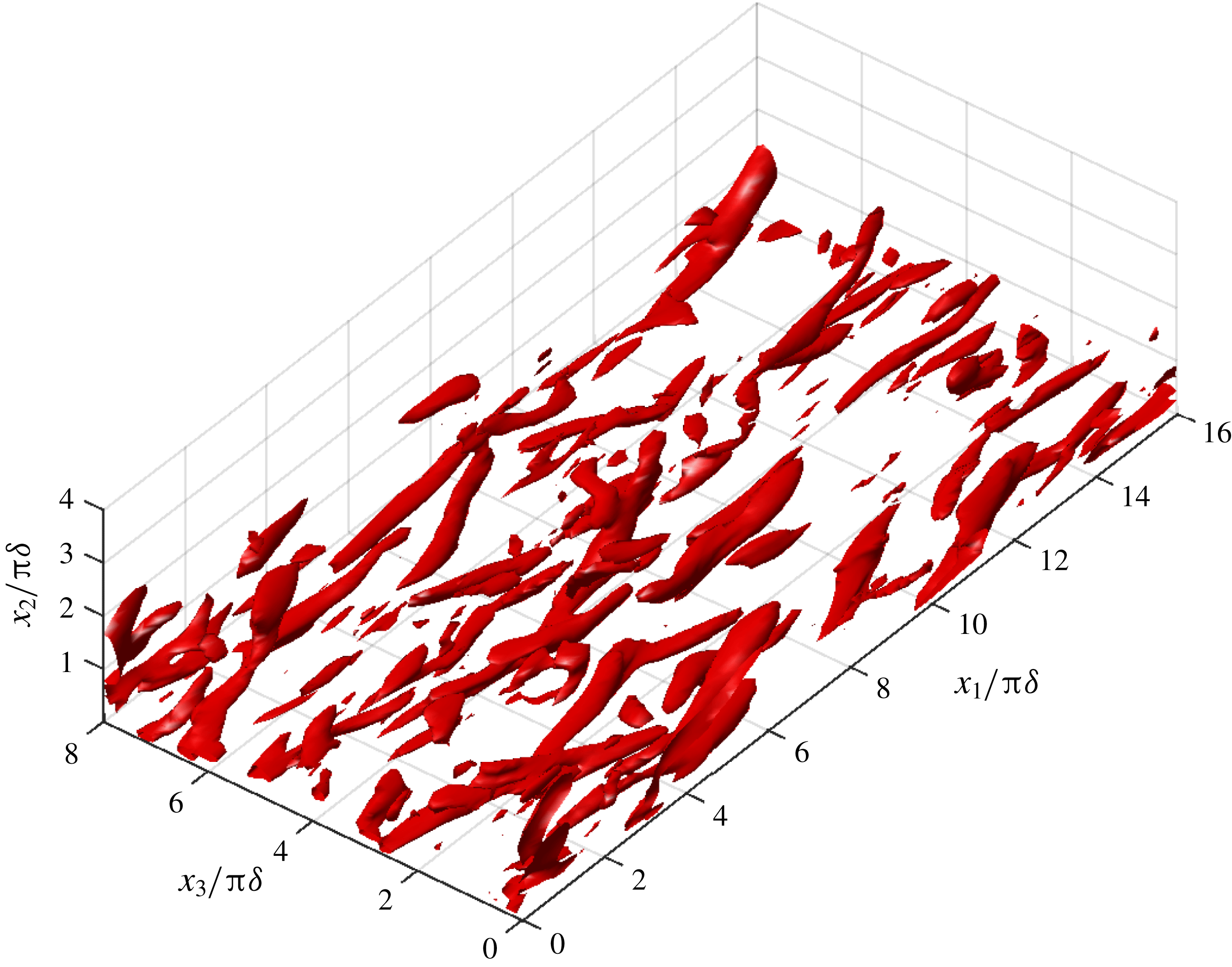
Iso-surfaces of
 $\langle Q\rangle$
at
 $\unicode[STIX]{x1D719}=180^{\circ }$
. The threshold is
 $Q_{m}\unicode[STIX]{x1D6FF}^{2}/U_{m}^{2}=1.6\times 10^{-3}$
.

Profile of
 $\langle Q\rangle$
during the cycle. Note the nonlinear scale of the vertical axis.

Statistics of wall pressure fluctuations
 $\tilde{p}_{0}$
. (a) Skewness; (b) kurtosis;
 $\unicode[STIX]{x1D6FE}_{1}$
and
 $\unicode[STIX]{x1D6FE}_{2}$
for normal distribution ——;
 $\cdots \cdots$
as in figure 5.

Wall pressure field. (a)
 $\unicode[STIX]{x1D719}=85^{\circ }$
; contours drawn for
 $[-6,6]~\text{Pa}$
at 1 Pa intervals. (b)
 $\unicode[STIX]{x1D719}=135^{\circ }$
; contours drawn for
 $[-4,4]~\text{Pa}$
at 0.5 Pa intervals. (c)
 $\unicode[STIX]{x1D719}=180^{\circ }$
; contours drawn for
 $[-10,10]~\text{Pa}$
at 1 Pa intervals. Dashed line: negative values; solid line: positive values.

Statistics of wall vorticity fluctuations
 $\unicode[STIX]{x1D6FA}^{\prime }/\unicode[STIX]{x1D6FA}_{rms}$
. (a) Skewness; (b) kurtosis; Dashed line
 $\unicode[STIX]{x1D6FA}_{1}$
; full line
 $\unicode[STIX]{x1D6FA}_{3}$
; ——
 $\unicode[STIX]{x1D6FE}_{1}$
and
 $\unicode[STIX]{x1D6FE}_{2}$
for normal distribution;
 $\cdots \cdots$
as in figure 5.

Wall streamwise vorticity field. (a)
 $\unicode[STIX]{x1D719}=85^{\circ }$
; contours drawn for
 $[-300,300]~\text{s}^{-1}$
at
 $50~\text{s}^{-1}$
intervals. (b)
 $\unicode[STIX]{x1D719}=135^{\circ }$
; contours drawn for
 $[-1800,1800]~\text{s}^{-1}$
at
 $300~\text{s}^{-1}$
intervals. (c)
 $\unicode[STIX]{x1D719}=180^{\circ }$
; contours drawn for
 $[-600,600]~\text{s}^{-1}$
at
 $100~\text{s}^{-1}$
intervals. Dashed line: negative values; solid line: positive values.

Wall spanwise vorticity field. (a)
 $\unicode[STIX]{x1D719}=85^{\circ }$
; contours drawn for
 $[0,3000]~\text{s}^{-1}$
at
 $250~\text{s}^{-1}$
intervals. (b)
 $\unicode[STIX]{x1D719}=135^{\circ }$
; contours drawn for
 $[0,3000]~\text{s}^{-1}$
at
 $250~\text{s}^{-1}$
intervals. (c)
 $\unicode[STIX]{x1D719}=180^{\circ }$
; contours drawn for
 $[-1200,0]~\text{s}^{-1}$
at
 $100~\text{s}^{-1}$
intervals. Dashed line: negative values; solid line: positive values.

Two point auto-correlation function at
 $x_{2}=0.5\unicode[STIX]{x1D6FF}$
(
 $x_{2}^{+}=10$
) in the spanwise directions for streamwise velocity component (solid line); spanwise velocity component (dashed line); wall normal velocity component (dash-dotted line). The spanwise lag is
 $r$
.

Time series of wall vorticity flux
 $\hat{\unicode[STIX]{x1D70E}}$
. Dotted line as in figure 5.

Statistics of boundary vorticity flux fluctuations
 $\unicode[STIX]{x1D70E}^{\prime }/\unicode[STIX]{x1D70E}_{rms}$
. (a) Skewness; (b) kurtosis; Dashed line
 $\unicode[STIX]{x1D70E}_{1}$
; full line
 $\unicode[STIX]{x1D70E}_{3}$
; ——
 $\unicode[STIX]{x1D6FE}_{1}$
and
 $\unicode[STIX]{x1D6FE}_{2}$
for normal distribution;
 $\cdots \cdots$
as in figure 5.

Wall vorticity flux at
 $\unicode[STIX]{x1D719}=85^{\circ }$
. (a) Streamwise component
 $\unicode[STIX]{x1D70E}_{1}$
; contours drawn for
 $[-1,2]~\text{m}~\text{s}^{-2}$
at
 $0.1~\text{m}~\text{s}^{-2}$
intervals. (b) Spanwise component
 $\unicode[STIX]{x1D70E}_{3}$
; contours drawn for
 $[-0.5,1]~\text{m}~\text{s}^{-2}$
at
 $0.1~\text{m}~\text{s}^{-2}$
intervals. Dashed line: negative values; solid line: positive values.

Wall vorticity flux at
 $\unicode[STIX]{x1D719}=135^{\circ }$
. (a) Streamwise component
 $\unicode[STIX]{x1D70E}_{1}$
; contours drawn for
 $[-10,10]~\text{m}~\text{s}^{-2}$
at
 $1~\text{m}~\text{s}^{-2}$
intervals. (b) Spanwise component
 $\unicode[STIX]{x1D70E}_{3}$
; contours drawn for
 $[-5,5]~\text{m}~\text{s}^{-2}$
at
 $0.5~\text{m}~\text{s}^{-2}$
intervals. Dashed line: negative values; solid line: positive values.

Wall vorticity flux at
 $\unicode[STIX]{x1D719}=180^{\circ }$
. (a) Streamwise component
 $\unicode[STIX]{x1D70E}_{1}$
; contours drawn for
 $[-1.5,1.5]~\text{m}~\text{s}^{-2}$
at
 $0.15~\text{m}~\text{s}^{-2}$
intervals. (b) Spanwise component
 $\unicode[STIX]{x1D70E}_{3}$
; contours drawn for
 $[-1,1]~\text{m}~\text{s}^{-2}$
at
 $0.1~\text{m}~\text{s}^{-2}$
intervals. Dashed line: negative values; solid line: positive values.

The solution was started with
 $p=0$
and
 $\boldsymbol{u}=0$
and ran for two cycles. Then a streamwise three-dimensional perturbation
 $u_{p}$
was added to the laminar velocity field:
 $$\begin{eqnarray}u_{p}=\unicode[STIX]{x1D700}U_{0}[a\cos (\unicode[STIX]{x1D6FC}x_{1})+b\cos (\unicode[STIX]{x1D6FD}x_{3})]\text{e}^{-\unicode[STIX]{x1D6FE}x_{2}^{2}},\end{eqnarray}$$
with
 $\unicode[STIX]{x1D6FC}=0.5$
and
 $\unicode[STIX]{x1D6FD}=1$
, corresponding to the most unstable combination of finite amplitude two-dimensional streamwise and spanwise perturbation of Akhavan et al. (Reference Akhavan, Kamm and Shapiro1991b
). The perturbation amplitudes were set to
 $a=5\times 10^{-3}$
and
 $b=10^{-7}$
. The exponential modulation coefficient is
 $\unicode[STIX]{x1D6FE}=5.5\times 10^{-4}$
and
 $\unicode[STIX]{x1D700}\ll 1$
is a random number uniformly distributed.
After the perturbation of the base laminar flow at
 $t^{\ast }=t/T=2$
, the flow reached the intermittently turbulent state within the following cycle. The simulation was then run for an additional eighteen cycles to build up a database for statistical analysis.
Checks on the grid spacings and domain size were performed to ensure that the results were not compromised by insufficient grid resolution or a too small domain size. To check requirement (i) the two-point velocity auto-correlations of the velocity field were computed for the streamwise and spanwise directions. All velocity components are decorrelated at lags lower than half of the domain lengths (figure 2).
Requirement (ii) was checked by computing the grid spacings. The spacings in wall units
 $\unicode[STIX]{x0394}x_{1}^{+}$
,
 $\unicode[STIX]{x0394}x_{2}^{+}$
and
 $\unicode[STIX]{x0394}x_{3}^{+}$
are
 $36$
,
 $0.4$
and
 $18$
, respectively, using the maximum value of the wall stress
 $\unicode[STIX]{x1D70F}_{0}$
to compute the wall scale
 $\unicode[STIX]{x1D708}/u_{\unicode[STIX]{x1D70F}}=\unicode[STIX]{x1D708}(\unicode[STIX]{x1D70F}_{0}/\unicode[STIX]{x1D70C})^{-1/2}$
. These values are adequate to resolve the elongated near-wall low-speed streaks (Salon et al.
Reference Salon, Armenio and Crise2007).
In addition, a grid convergence check was performed to verify the grid independence of the results by running additional simulations with increased grid node count in the streamwise and spanwise directions to 128 and in the wall normal direction to 192 nodes (table 1). The simulations were run on the Fionn supercomputer of the Irish Centre for High-End Computing (ICHEC) using 96 cores. Due to the high computational cost, only partial computations were performed with the highly refined meshes C2 and C3.
Grid size and resolution of the simulations. Wall units (
 $^{+}$
) are based on the minimum value of the wall scale
 $\unicode[STIX]{x1D708}/u_{\unicode[STIX]{x1D70F}}$
(maximum value of the shear velocity
 $u_{\unicode[STIX]{x1D70F}}$
).

The evolution of the wall shear stress (figure 3
a) does not show appreciable variations during the turbulent phase of the cycle. Although grid C1 shows higher wall shear during the middle acceleration stage, the maximum level of non-dimensional wall shear stress has converged to the values of 1.04, 1.01 and 1.08 for the C1, C2 and C3 simulations. The profile of the streamwise mean velocity (figure 3
b) also shows a convergence between all three grids, with C2 closer to the experimental results. The results of the grid spacing and domain size checks, together with the grid convergence test, show that the grid C1 is capable of capturing the dynamics of the Stokes boundary layer at
 $Re_{\unicode[STIX]{x1D6FF}}=1000$
.
4 Results
Given the oscillatory nature of the flow a simple ensemble averaging is not meaningful. Instead, an ensemble phase averaging is used to produce meaningful average properties. For quantity
 $f$
, the ensemble phase average is
 $$\begin{eqnarray}\langle f(x_{2},\unicode[STIX]{x1D719})\rangle =\frac{1}{N}\mathop{\sum }_{i=1}^{N}\left\{\frac{1}{L_{1}L_{3}}\iint f(x_{1},x_{2},x_{3},t+(i-1)T)\,\text{d}x_{1}\,\text{d}x_{3}\right\},\end{eqnarray}$$
where
 $\unicode[STIX]{x1D719}=\unicode[STIX]{x1D714}t$
is the phase,
 $T$
is the period and
 $N$
is the number of cycles. The fluctuating (turbulent) part of
 $f$
is then
 $f^{\prime }=f-\langle f\rangle$
. For quantities defined on the solid wall, the spatial average is done for
 $x_{2}=0$
only.
Magnitudes of quantities that fluctuate in space and time were measured by the root mean square (r.m.s.) value that is defined as
 $$\begin{eqnarray}\hat{f}=\sqrt{\frac{1}{L_{1}L_{3}}\iint (f^{\prime })^{2}\,\text{d}x_{1}\,\text{d}x_{3}}\end{eqnarray}$$
for scalar quantities defined only on the solid wall; the vector norm is used for vector quantities. For quantities defined in the whole domain the spatial averaging changes accordingly. The change in r.m.s. intensity along the cycle is computed by performing an additional phase averaging on
 $\hat{f}(t)$
.
The phase averaged probability density function (p.d.f.)
 $B(\tilde{f})$
of the normalized fluctuations
 $\tilde{f}=f^{\prime }/\hat{f}$
, was calculated by phase averaging the instantaneous pdf
 $b(\tilde{f})$
. The shape parameters skewness (
 $\unicode[STIX]{x1D6FE}_{1}$
) and kurtosis (
 $\unicode[STIX]{x1D6FE}_{2}$
) were computed from
 $B(\tilde{f})$
as:
 $$\begin{eqnarray}\displaystyle & \displaystyle \unicode[STIX]{x1D6FE}_{1}=\frac{1}{\unicode[STIX]{x1D70E}^{3}}\int \tilde{f}^{3}B(\tilde{f})\,\text{d}\tilde{f}; & \displaystyle\end{eqnarray}$$
 $$\begin{eqnarray}\displaystyle & \displaystyle \unicode[STIX]{x1D6FE}_{2}=\frac{1}{\unicode[STIX]{x1D70E}^{4}}\int \tilde{f}^{4}B(\tilde{f})\,\text{d}\tilde{f}. & \displaystyle\end{eqnarray}$$
In (4.3) and (4.4),
 $\unicode[STIX]{x1D70E}$
is the standard deviation of
 $B(\tilde{f})$
.
4.1 Turbulence characteristics
The numerical simulations produced flow fields that exhibit the characteristics observed in experimental studies of the Stokes boundary layer at
 $Re_{\unicode[STIX]{x1D6FF}}\sim 1000$
, in the IT regime. The velocity components exhibit sudden high amplitude random three-dimensional fluctuations at the beginning of the deceleration stage (figure 4), indicating the transition to turbulence that is known to occur at this stage of the cycle. Towards the end of the deceleration stage, the intensity of these fluctuations decreases and the flow reaches a quasi-laminar state during the accelerating stage.
The volume integrated turbulent kinetic energy:
 $$\begin{eqnarray}{\mathcal{E}}=\frac{1}{V}\int (u_{1}^{\prime 2}+u_{2}^{\prime 2}+u_{3}^{\prime 2})\,\text{d}V\end{eqnarray}$$
rises rapidly in the late acceleration stage and reaches a maximum in the early deceleration stage (figure 5
a). The rise in
 ${\mathcal{E}}$
coincides with the sudden appearance of large velocity fluctuations and is thought to be associated with the mechanism of near-wall shear instability at the start of the deceleration stage that is sustained by the burst mechanism (Hino et al.
Reference Hino, Kashiwayanagi, Nakayama and Hara1983).
The wall shear stress
 $\unicode[STIX]{x1D70F}_{0}$
(figure 5
b), slowly increases from
 $\unicode[STIX]{x1D719}=0^{\circ }$
, reaching a first plateau at the phase of maximum velocity and then rapidly increases up to an absolute maximum at the phase of maximum turbulent motion. At this point it is worth mentioning that as
 $Re_{\unicode[STIX]{x1D6FF}}$
increases from the laminar range, the phase profile of
 $\unicode[STIX]{x1D70F}_{0}$
changes accordingly: in the laminar regime, it follows the
 $\cos (\unicode[STIX]{x1D714}t-\unicode[STIX]{x03C0}/4)$
solution of (Batchelor Reference Batchelor2000); as
 $Re_{\unicode[STIX]{x1D6FF}}$
increases into the IT regime, the onset of turbulence at the early phases of the deceleration stage creates the profile observed in figure 5(b); further increase of
 $Re$
causes the maximum to appear earlier, aided by the adverse pressure gradient and when the phase of maximum
 $\unicode[STIX]{x1D70F}_{0}$
falls below
 $\unicode[STIX]{x03C0}/2$
in to the acceleration stage, the change of the
 $\unicode[STIX]{x1D70F}_{0}$
is deterred by the favourable pressure gradient (Jensen et al.
Reference Jensen, Sumer and Fredsøe1989).
A logarithmic layer develops in the mean velocity profile (figure 6), as reported in earlier experimental studies (Hino et al.
Reference Hino, Kashiwayanagi, Nakayama and Hara1983; Jensen et al.
Reference Jensen, Sumer and Fredsøe1989; Akhavan, Kamm & Shapiro Reference Akhavan, Kamm and Shapiro1991a
). The mean profiles for the deceleration stage conform to a 3-layer structure of a viscous sublayer, a log layer, whose thickness increases as
 $\unicode[STIX]{x1D719}$
advances and an outer wake.
The rapid increase of
 $\left(u_{1}^{\prime }\right)_{rms}/U_{0}$
in the near-wall region at the end of the acceleration stage and through the deceleration stage of the cycle (figure 7), signals the onset of turbulence in the near-wall region. The wall normal r.m.s. fluctuations (figure 8) increase during the turbulent phases of the cycle (between
 $70^{\circ }$
and
 $140^{\circ }$
). Comparing to the experimental results of Jensen et al. (Reference Jensen, Sumer and Fredsøe1989), the DNS results overestimate the wall normal turbulence intensity, except in the initial phases of the turbulence, where they underestimate the r.m.s. of
 $u_{2}^{\prime }$
(figure 8
c).
Profiles of the Reynolds stress
 $u_{1}^{\prime }u_{2}^{\prime }$
are shown in figure 9. The simulated turbulent stresses are compared to the ones from Test 6 of Jensen et al. (Reference Jensen, Sumer and Fredsøe1989) and the agreement is quite reasonable. It can be seen that turbulence reaches its highest intensities around
 $\unicode[STIX]{x1D719}=107^{\circ }$
, in agreement with the data on turbulent kinetic energy and wall shear stress of figure 5.
In general the experimental results support the numerical simulations but some discrepancies between the numerical results and the experimental data can be observed at
 $\unicode[STIX]{x1D719}=73^{\circ }$
and
 $\unicode[STIX]{x1D719}=107^{\circ }$
(panels c and d of figures 7–9), in the central part of the half-cycle. Costamagna et al. (Reference Costamagna, Vittori and Blondeaux2003) also found similar discrepancies and attributed them to the small size of the domain, but later Salon et al. (Reference Salon, Armenio and Crise2007) also found similar deviations in the streamwise turbulence intensity for the central part of the cycle but for a larger domain and discarded that the cause could be domain size. The reason for these discrepancies remains unclear and further research is necessary to clarify the source of these errors.
4.2 Coherent structures
In the IT regime of the Stokes boundary layer, coherent structures appear at particular phases of the cycle, unlike the steady boundary layer case, where these appear randomly in time. To identify them we use the
 $Q$
-criterion (Dubief & Delcayre Reference Dubief and Delcayre2000):
 $$\begin{eqnarray}Q={\textstyle \frac{1}{2}}(\unicode[STIX]{x1D64D}\boldsymbol{ : }\unicode[STIX]{x1D64D}-\unicode[STIX]{x1D64E}\boldsymbol{ : }\unicode[STIX]{x1D64E}),\end{eqnarray}$$
where
 $\unicode[STIX]{x1D64D}$
and
 $\unicode[STIX]{x1D64E}$
are the antisymmetric and symmetric parts of
 $\unicode[STIX]{x1D735}\boldsymbol{u}$
. The scalar
 $Q$
is the difference between the rotation rate and strain rate and gives a measure of the local dominance of rotation over strain (
 $Q>0$
) or vice versa (
 $Q<0$
). Large positive values of
 $Q$
are related to vortical coherent structures (regions of coherent vorticity) and large negative values of
 $Q$
indicate shear coherent structures. To delineate the boundaries of the structures, a threshold of
 $Q$
must be chosen. This choice of threshold has a degree of subjectivity: a too high threshold will result only in partial structures while a too low threshold will produce too many small-scale, weak features with no real impact on the dynamics (Dubief & Delcayre Reference Dubief and Delcayre2000). The threshold used in this paper,
 $Q_{m}$
, is the value of
 $Q$
at the ninth decile level, based on the phase-mean
 $Q$
fields,
 $\langle Q\rangle$
. At this level, the 10 % highest values of
 $\langle Q\rangle$
are inside the iso-surfaces of
 $Q_{m}$
.
The coherent structures for
 $\unicode[STIX]{x1D719}=85^{\circ }$
show an organization of the Stokes layer in long vortical cores located close to the wall (figure 10). This organization corresponds to that described by Scotti & Piomelli (Reference Scotti and Piomelli2001) for the pulsating turbulent channel flow, where at
 $T/4$
the near-wall flow is organized in long and smooth streaks; and to the findings of Costamagna et al. (Reference Costamagna, Vittori and Blondeaux2003), that for the late acceleration stage found low-speed streaks, associated with high values of
 $\unicode[STIX]{x1D6FA}_{3}$
. The streaks appear as a consequence of the alignment of spanwise vortices of the same sign, as the flow decelerates, and originate the long vortex structures educed by the
 $\langle Q\rangle$
field (Costamagna et al.
Reference Costamagna, Vittori and Blondeaux2003).
In the later stages of the cycle, the vortical coherent structures loose their elongated shape. At
 $\unicode[STIX]{x1D719}=135^{\circ }$
(figure 11), the strong vortical regions appear as short and slightly upward tilted, with an orientation that is still clearly streamwise. At the end of the deceleration stage (
 $\unicode[STIX]{x1D719}=180^{\circ }$
, figure 12), the coherent structures have lost their streamwise orientation and are tilted away from the wall. This occurs simultaneously with an upward progression of the vortical structures that move away from the wall, as noticed also by Costamagna et al. (Reference Costamagna, Vittori and Blondeaux2003) using tracer trajectories.
The absolute value of the wall normal profile of
 $\langle Q\rangle$
reaches a minimum at
 $\unicode[STIX]{x1D719}=45^{\circ }$
and
 $\unicode[STIX]{x1D719}=225^{\circ }$
, half-way through the acceleration stage (figure 13). It then increases until reaching the maximum shortly after the beginning of the deceleration stage. Throughout the cycle, the profile of
 $\langle Q\rangle$
remains unaltered: close to the wall (
 $x_{2}/\unicode[STIX]{x03C0}\unicode[STIX]{x1D6FF}<0.2$
), straining dominates rotation and the high vorticity found at the wall is due to the straining of the fluid, probably by the large-scale flow; between
 $0.2<x_{2}/\unicode[STIX]{x03C0}\unicode[STIX]{x1D6FF}<1$
, rotation dominates and above
 $x_{2}/\unicode[STIX]{x03C0}\unicode[STIX]{x1D6FF}=1$
, there appears to be a balance between strain and rotation.
4.3 Wall pressure
The evolution of the skewness of the normalized wall pressure fluctuations
 $\tilde{p}_{0}=p_{0}^{\prime }/\hat{p}_{0}$
along the cycle (figure 14
a) can be divided in two zones:
 $\unicode[STIX]{x1D6FE}_{1}$
grows from 0 (the value for a Gaussian distribution) up to a value of
 $0.2\sim 0.4$
during the acceleration stage and then starts to decline to the Gaussian value at the end of the acceleration stage and during the deceleration stage, where large excursions between positive and negative
 $\unicode[STIX]{x1D6FE}_{1}$
are present. The positive
 $\unicode[STIX]{x1D6FE}_{1}$
of the accelerating stage indicates that high negative values of
 $\tilde{p}_{0}$
are more likely to occur than high positive values. During the late acceleration and early deceleration stages, when turbulence appears and reaches its maximum intensity,
 $\unicode[STIX]{x1D6FE}_{1}$
apparently decreases to a Gaussian value on average while attaining large negative and positive values from phase to phase. This is in disagreement with the experimental studies in permanent turbulent boundary layers of Schewe (Reference Schewe1983) and Andreopoulos & Agui (Reference Andreopoulos and Agui1996) and the numerical study of Kim (Reference Kim1989), who found that
 $\unicode[STIX]{x1D6FE}_{1}$
of pressure fluctuations at the wall was
 ${\sim}-0.2$
.
The kurtosis of
 $\tilde{p}_{0}$
(figure 14
b) shows maxima of
 $4\sim 5$
at the inception of turbulence in the cycle. During the acceleration stage
 $\unicode[STIX]{x1D6FE}_{2}$
rises from
 ${\sim}2.5$
in the early phases of this stage and after the peak,
 $\unicode[STIX]{x1D6FE}_{2}$
decreases during the deceleration stage. During the late deceleration stage and the early acceleration stage,
 $\unicode[STIX]{x1D6FE}_{2}$
is lower than that of a Gaussian distribution (
 $\unicode[STIX]{x1D6FE}_{2}=3$
), while the inverse is true during the late acceleration and early deceleration stages. The maximum values of
 $\unicode[STIX]{x1D6FE}_{2}$
are in line with the experimental and numerical results reported in the literature, e.g.
 $\unicode[STIX]{x1D6FE}_{2}=4.19$
by Schewe (Reference Schewe1983). This high value of
 $\unicode[STIX]{x1D6FE}_{2}$
means that extremely high or low amplitudes occur more often than in a Gaussian distribution.
In the late acceleration stage (
 $\unicode[STIX]{x1D719}=85^{\circ }$
), the wall pressure distribution (figure 15
a), is predominantly negative, although positive pressure peaks are also visible. Large spanwise pressure gradients can be observed next to the positive pressure peaks (e.g. at
 $x_{3}\sim 2\unicode[STIX]{x03C0}\unicode[STIX]{x1D6FF}$
and
 $10\unicode[STIX]{x03C0}\unicode[STIX]{x1D6FF}<x_{1}<14\unicode[STIX]{x03C0}\unicode[STIX]{x1D6FF}$
). At
 $\unicode[STIX]{x1D719}=135^{\circ }$
(deceleration stage), the wall pressure distribution has changed considerably (figure 15
b). Positive and negative pressures are more evenly distributed but the negative pressure peaks become more frequent. However, these characteristics can change rapidly between successive phases as suggested by the highly fluctuating behaviour of the skewness in this region of the cycle. At the end of the deceleration stage (
 $\unicode[STIX]{x1D719}=180^{\circ }$
), the pressure distribution largely exhibits negative values on the wall with isolated regions of positive pressure (figure 15
c). The similarities with the distribution at
 $\unicode[STIX]{x1D719}=85^{\circ }$
are evident and looking at the evolution of the skewness during the acceleration stage of cycle the main change to expect is the increase in the number of negative pressure peaks.
Observing the wall pressure distributions, the behaviour of the kurtosis may be explained by noting that while for the late acceleration stage the extreme values occupy a small fraction of the wall, for the remainder of the cycle the extremes of the distribution occupy a much larger fraction of the total wall region.
4.4 Wall vorticity
Due to the no-slip condition, velocity gradients in the
 $x_{1}$
and
 $x_{3}$
direction are zero and the normal component of vorticity
 $\unicode[STIX]{x1D6FA}_{2}$
is therefore also zero.
The skewness of the
 $\unicode[STIX]{x1D6FA}_{1}$
and
 $\unicode[STIX]{x1D6FA}_{3}$
components (figure 16
a) show very distinct behaviours. The
 $\unicode[STIX]{x1D6FE}_{1}$
for
 $\unicode[STIX]{x1D6FA}_{1}$
is very close to the Gaussian value and is much lower than
 $\unicode[STIX]{x1D6FE}_{1}$
for
 $\unicode[STIX]{x1D6FA}_{3}$
. This last component has positive
 $\unicode[STIX]{x1D6FE}_{1}$
during the first half-cycle and negative during the second half-cycle. The
 $\unicode[STIX]{x1D6FA}_{3}$
skewness starts with a positive value
 ${\sim}0.3$
rising up to
 ${\sim}0.5$
before
 $\unicode[STIX]{x1D719}=15^{\circ }$
and then starts to decline until
 $\unicode[STIX]{x1D719}=60^{\circ }$
, when it experiences a sharp increase, reaching a maximum of
 $O(1)$
slightly before the end of the acceleration phase; after this peak, it slowly declines during the turbulent phase of the cycle until approximately
 $\unicode[STIX]{x1D719}=165^{\circ }$
, when it experiences a rapid transition to the subsequent half-cycle where its sign is reversed. This indicates a strong influence of the driving flow on the spanwise wall vorticity distribution and has direct consequences on the shedding of positive or negative vorticity.
In the late acceleration stage (
 $\unicode[STIX]{x1D719}=85^{\circ }$
, figure 17
a) the
 $\unicode[STIX]{x1D6FA}_{1}$
field shows elongated vortex structures in the streamwise direction, while in the spanwise direction we observe alternating zones of positive and negative
 $\unicode[STIX]{x1D6FA}_{1}$
. Since
 $u_{3}=\unicode[STIX]{x1D6FA}_{1}dx_{2}$
, the field is strongly related to the spanwise velocity field at short distances above the wall. The elongated and alternating
 $\unicode[STIX]{x1D6FA}_{1}$
features thus seem to be the result of near-wall counter-rotating vortices aligned in the streamwise direction. These streamwise vortices result from the stretching of patches of streamwise vorticity by the large wall normal gradients of streamwise velocity (Costamagna et al.
Reference Costamagna, Vittori and Blondeaux2003). The small
 $\unicode[STIX]{x1D6FE}_{1}$
indicates that the field of counter-rotating streamwise vortices has with the same likelihood positive and negative signs, while the high
 $\unicode[STIX]{x1D6FE}_{2}$
is a result of the elongated nature of the structures.
In the deceleration stage (
 $\unicode[STIX]{x1D719}=135^{\circ }$
, figure 17
b) the stream wise vorticity field has lost the streamwise organization of the late acceleration stage, thereby exhibiting a lower
 $\unicode[STIX]{x1D6FE}_{2}$
, while the number of high positive and negative peaks remains similar (
 $\unicode[STIX]{x1D6FE}_{1}$
maintains a Gaussian magnitude).
In the late acceleration stage the spanwise vorticity field exhibits alternating regions of low and high vorticity (figure 18
b). At the wall we have
 $\unicode[STIX]{x1D6FA}_{3}=-\unicode[STIX]{x2202}u_{1}/\unicode[STIX]{x2202}x_{2}$
so the wall distribution of
 $\unicode[STIX]{x1D6FA}_{3}$
signals that the near-wall streamwise velocity field is organized in alternating low and high speed regions, the so called streaks, already observed for the steady turbulent boundary layer and oscillating boundary layer (see Costamagna et al. (Reference Costamagna, Vittori and Blondeaux2003) and references there in).
To estimate the spacing of the low-speed streaks, the spanwise two-point auto-correlation function of the velocity field was computed for the phase
 $\unicode[STIX]{x1D719}=85^{\circ }$
at the distance of
 $0.5\unicode[STIX]{x1D6FF}$
from the wall. The streamwise low-speed streak spacing is estimated as the decorrelation length of the streamwise velocity, about
 $1.5\unicode[STIX]{x03C0}\unicode[STIX]{x1D6FF}$
(figure 19). In the subsequent evolution of the spanwise wall vorticity field, we observe the loss of the streamwise homogeneity with the appearance of a wavy pattern and after that the breakdown into small patches of streamwise vorticity, as described by Costamagna et al. (Reference Costamagna, Vittori and Blondeaux2003). Note that contrary to the
 $\unicode[STIX]{x1D6FA}_{1}$
component, the kurtosis of the
 $\unicode[STIX]{x1D6FA}_{1}$
component remains close to Gaussian.
4.5 Dynamics of the boundary vorticity flux
In the case of a flat, stationary wall
 $\unicode[STIX]{x1D748}_{a}$
and
 $\unicode[STIX]{x1D748}_{\unicode[STIX]{x03C0}}$
vanish. Moreover, the dot product in (2.8d
) is between orthogonal vectors so
 $\unicode[STIX]{x1D748}_{n}$
vanishes equally and only the pressure component
 $\unicode[STIX]{x1D748}_{p}$
is non-zero. The r.m.s. of the pressure component (figure 20) reaches its maximum values at the peak of the turbulent motions (the maxima of
 ${\mathcal{E}}$
), in the beginning of the deceleration phase. Outside of this range of phases,
 $\hat{\unicode[STIX]{x1D70E}}_{p}$
rapidly drops and remains low during the acceleration stage of the cycle.
The streamwise and spanwise components of
 $\unicode[STIX]{x1D748}$
are due to the wall pressure gradients:
 $$\begin{eqnarray}\unicode[STIX]{x1D748}=\left(\frac{\unicode[STIX]{x2202}p}{\unicode[STIX]{x2202}x_{3}}\right)\boldsymbol{i}_{\mathbf{1}}-\left(\frac{\unicode[STIX]{x2202}p}{\unicode[STIX]{x2202}x_{1}}\right)\boldsymbol{i}_{\mathbf{3}}.\end{eqnarray}$$
The skewness and kurtosis of the wall vorticity flux components were computed using the p.d.f. of
 $\tilde{\unicode[STIX]{x1D70E}}$
(figure 21). Instantaneous maps of
 $\unicode[STIX]{x1D70E}_{1}$
and
 $\unicode[STIX]{x1D70E}_{3}$
are shown in figures 22–24.
In the late acceleration stage, the vorticity flux in the streamwise direction is organized in elongated regions with sharp variations in the spanwise direction (figure 22
a). The strongest
 $\unicode[STIX]{x1D70E}_{1}$
occurs in the region of the sharp spanwise pressure gradient identified above (figure 15
a). In this phase the skewness is positive indicating the more likely occurrence of high negative values of
 $\unicode[STIX]{x1D70E}_{1}$
, but in general the
 $\unicode[STIX]{x1D70E}_{1}$
skewness oscillates heavily between positive and negative values (figure 21
a) during the cycle. Kurtosis is high in this stage of the cycle due to the elongated configuration of
 $\unicode[STIX]{x1D70E}_{1}$
. The spanwise component of
 $\unicode[STIX]{x1D70E}$
shows a different distribution at the end of the acceleration stage (figure 22
b). The extremes are concentrated in small regions of the wall but the field does not possess the elongated character of
 $\unicode[STIX]{x1D70E}_{1}$
, hence the lower kurtosis. Again the wall vorticity flux is clearly connected to the pressure gradient (streamwise in this case), as the peaks in the
 $\unicode[STIX]{x1D70E}_{3}$
field match the sharp variations in the pressure signal in the streamwise direction figure 15(a).
In the deceleration stage (figure 23
a), the
 $\unicode[STIX]{x1D70E}_{1}$
field has lost streamwise coherence and exhibits much greater variations in this direction. This is due to the similar number of positive and negative wall pressure peaks and so sharp wall pressure gradients are more evenly distributed throughout the wall. Indeed, the streamwise decorrelation length scale
 $r/\unicode[STIX]{x03C0}\unicode[STIX]{x1D6FF}$
of the wall pressure field decreases to 1–3, from 4–6 during the acceleration stage, and thus the spatial correlation of the pressure signal is lower and therefore an increase in the wall vorticity flux level is to be expected (Andreopoulos & Agui Reference Andreopoulos and Agui1996). The spanwise wall vorticity flux field (figure 23
b) has a structure very similar to the streamwise field at this phase with similar kurtosis, although with a higher negative skewness (figure 21
a). This is an important finding since it reveals a sustained process of production of strong positive and negative wall pressures during this stage of the cycle (figure 15
b), generating large streamwise pressure gradients and enhancing the spanwise wall vorticity flux. Again, it is seen that the spanwise vorticity is the most affected by the flow oscillations. A likely cause is the repeated and widespread occurrence of the sweep/ejection event that was found to be associated with high values of the wall vorticity flux (Andreopoulos & Agui Reference Andreopoulos and Agui1996). At the end of the deceleration stage (figure 24)
 $\unicode[STIX]{x1D70E}_{1}$
presents a spatial distribution similar to the one found for
 $\unicode[STIX]{x1D719}=135^{\circ }$
. On the other hand, a substantially different distribution is found for
 $\unicode[STIX]{x1D70E}_{3}$
at this stage. The correlation between pressure values is larger than in the previous case and the extreme values are mostly positive and are spatially related to negative streamwise pressure gradients.
5 Conclusions
The Stokes layer shows different regimes of flow, depending on the frequency of oscillation, the free-stream velocity and the fluid properties. For low free-stream speeds or high oscillation frequencies (low
 $Re_{\unicode[STIX]{x1D6FF}}$
), the flow is laminar and the wall shear stress obeys a cosine type law with a
 $\unicode[STIX]{x03C0}/4$
phase lag in relation to the free-stream oscillation. As
 $Re_{\unicode[STIX]{x1D6FF}}$
increases, turbulence appears in the deceleration stage of the cycle but is suppressed during the acceleration phase (the IT regime) until
 $Re_{\unicode[STIX]{x1D6FF}}$
is high enough so as to have turbulence in the entire cycle. During this evolution with
 $Re_{\unicode[STIX]{x1D6FF}}$
, the wall friction behaviour changes as the relative strengths of turbulent stresses and pressure gradient change.
The DNS reported here were able to reproduce the characteristics of the Stokes layer cycle in the IT regime that have been identified in previous experimental and numerical studies. In particular, the cycle exhibits the sudden appearance of turbulent motions in the early moments of the deceleration stage of the cycle and their almost complete suppression during the acceleration stage and the appearance, thickening and disappearance of a log layer in the near wall mean velocity profile.
The statistics of wall pressure (skewness and kurtosis) vary considerably during the cycle, due to the change in sign of the predominant wall pressure fluctuations and the relative number of extreme fluctuations in wall pressure. On average, during the turbulent phase of the cycle, positive and negative extremes are equally likely to occur but at the same time, very high values of pressure fluctuations are less likely as the deceleration stage progresses. Vorticity statistics show also a variation along the cycle, except for the skewness of the streamwise component that oscillates mildly around zero throughout the cycle. Differences in these statistics, similar to the ones found for canonical boundary layers (see Honkan & Andreopoulos (Reference Honkan and Andreopoulos1997)) support the view that vorticity is subject to the same influences from coherent structures as in the permanent boundary layer case. Observation of instantaneous vorticity fields in this work and others (Costamagna et al. Reference Costamagna, Vittori and Blondeaux2003) further support this hypothesis.
At the wall, pressure and vorticity are intimately related by the wall vorticity flux since the pressure gradient is the source of the wall vorticity flux. During the oscillatory cycle, the maximum of
 $\unicode[STIX]{x1D748}$
coincides with the turbulent kinetic energy maximum. Instantaneous distributions show a close connection to the pressure distribution, as could be expected. Indeed, the relationship between wall pressure and vorticity is intricate since the newly created wall vorticity is diffused into the fluid, and then moved away from the wall, where it will modify the turbulence structures that created the pressure distributions at the wall, thereby changing the flux of vorticity at the wall.
When considering viscous flow around a wave energy device, these results show that the wall vorticity distribution, that is shed from the sharp edges of the device and is entrained in the flow, will exhibit different characteristics according to the phase of the cycle. This is especially true for the spanwise vorticity component that is affected to a higher degree by the flow oscillation. This variation in the wall vorticity distribution will influence the subsequent stages of the device motions, due to its effects on the overall force balance. In the case of the wave energy devices the phase of the cycle is determined not only by the ambient flow but also by the motion of the device itself, which will feedback into the vorticity sheet characteristics. This interaction between ambient flow, wall vorticity, global forces and device motion is especially important during extreme events, where viscous loads are known to be significant. Further work is required to gain a better insight into this process and, in particular, we plan to extend the analysis in a setting where a vorticity sheet shedding from a sharp corner occurs.
Acknowledgements
This material is supported by the Science Foundation Ireland (SFI) under grant number SFI/12/RC/2302. The authors would like to thank the Irish Centre for High-End Computing for the provision of computational facilities and support and the assistance of ICHEC staff during the runs in the Fionn supercomputer.



