


1 Introduction
Gravity (or density) currents (GCs) spread out every time that a fluid propagates into an ambient and the flow is driven by a density difference. This type of flow has both geophysical and industrial applications, such as saltwater wedges in estuaries, oil spills in the ocean, magma and lava flows, dredge disposal and industrial gas release; numerous examples are illustrated by Simpson (Reference Simpson1997).
A stringent classification of gravity currents is related to the main balance dominating the flow, either inertial–buoyancy or viscous–buoyancy.
In a two-dimensional geometry, both inertial and viscous currents of volume
 $qt^{\unicode[STIX]{x1D6FF}}$
,
 $q>0$
,
 $\unicode[STIX]{x1D6FF}\geqslant 0$
, display self-similar propagation of the form
 $x_{N}=K_{i}t^{\unicode[STIX]{x1D6FD}_{i}}$
, where
 $i=I,V$
for the inertial and the viscous regimes respectively. In general,
 $\unicode[STIX]{x1D6FD}_{i}$
increases with
 $\unicode[STIX]{x1D6FF}$
(Didden & Maxworthy (Reference Didden and Maxworthy1982), Huppert (Reference Huppert1982); see also Ungarish (Reference Ungarish2009) § 4.2). Since the GC is a strongly time-dependent phenomenon, a downstream change of dynamic regime may occur at some distance from the injection section. For the more common occurrence
 $\unicode[STIX]{x1D6FF}<7/4$
(subcritical case), the transition is between the inertial and viscous regimes, and is manifested by a decrease of the
 $\unicode[STIX]{x1D6FD}$
exponent. There is, however, an interesting ‘critical’ exception: the theory predicts that for
 $\unicode[STIX]{x1D6FF}=7/4$
,
 $\unicode[STIX]{x1D6FD}_{I}=\unicode[STIX]{x1D6FD}_{V}=5/4$
, and hence a regime transition is impossible. A two-dimensional (2-D) current sustained by the critical exponent of the influx rate
 $\unicode[STIX]{x1D6FF}_{c}=7/4$
is expected to maintain the original flow regime for a very long time; in practice, the nature of the flow will eventually be changed by some obstacle, or by the turn-off of the injection source. This fixed-force regime is characterized by a fixed effective Reynolds number
 $Re_{e}=(q^{2}/g^{\prime })^{2/3}/\unicode[STIX]{x1D708}$
, where
 $g^{\prime }$
is the reduced gravity and
 $\unicode[STIX]{x1D708}$
is the kinematic viscosity (we note in passing that the third power of the inverse of this number has been defined as the Julian number,
 $J$
, but we think that
 $Re_{e}$
is a more insightful parameter). These theoretical predictions were confirmed by stringent experimental tests conducted by Maxworthy (Reference Maxworthy1983).
The ‘critical’ fixed-force regime behaviour has been considered as a strong achievement of gravity current investigations. Here, the theoretical tools for inertial and viscous currents combine with experimental skill into sharp unexpected insights and results. The available theoretical formulation for critical gravity currents is restricted to channels of rectangular, or infinitely wide, cross-section. The objective of the present investigation is to determine whether and how the ‘critical’ effect of the constant force regime can be generalized to gravity currents in non-rectangular channels.
An extension to channels of non-rectangular cross-section represents an important theoretical advancement as it implies an increase in domain dimensionality and incorporates three-dimensional (3-D) effects (Longo et al. Reference Longo, Ungarish, Di Federico, Chiapponi and Maranzoni2015b , Reference Longo, Ungarish, Di Federico, Chiapponi and Addona2016b ). Furthermore, the inclusion of stratification effects in the ambient fluid extends the investigation to an important class of non-homogeneous fluids, whose association with gravity flows produces striking phenomena (Longo et al. Reference Longo, Ungarish, Di Federico, Chiapponi and Addona2016a ).
For inertial currents, the effects of non-rectangular cross-section channels were investigated by Monaghan et al. (Reference Monaghan, Mériaux, Huppert and Monaghan2009), Marino & Thomas (Reference Marino and Thomas2011) and Zemach & Ungarish (Reference Zemach and Ungarish2013); the effect of a linear stratification was incorporated into the model by Ungarish (Reference Ungarish2015). Viscous gravity currents propagating into non-rectangular cross-sections filled with homogeneous ambient fluid were modelled by Takagi & Huppert (Reference Takagi and Huppert2007, Reference Takagi and Huppert2008); to the best of our knowledge, the joint effect of viscosity and stratification has not been considered in the literature. A modelling effort to incorporate non-Newtonian effects was undertaken by Longo, Di Federico & Chiapponi (Reference Longo, Di Federico and Chiapponi2015a ). See Ungarish (Reference Ungarish2018) for a short review.
The simplified thin-layer equations (of shallow-water type for an inertial–buoyancy current and lubrication type for a viscous–buoyancy current) are partial differential with respect to time
 $t$
and length
 $x$
, and in general require numerical solution. However, it turns out that for channels of power-law cross-section
 $f(z)=bz^{\unicode[STIX]{x1D6FC}}$
, these equations admit similarity solutions, and the resulting propagation is of the form
 $x_{N}=Kt^{\unicode[STIX]{x1D6FD}}$
for a variety of boundary conditions. (Here,
 $z$
is the vertical coordinate and
 $K$
is a coefficient depending on several parameters of the current; the 2-D rectangular cross-section is just a particular case, corresponding to
 $\unicode[STIX]{x1D6FC}=0$
.) This type of solution is a very convenient (and to the best of our knowledge the only rigorous) tool for analytical investigation of long-time (or long-distance) propagation of gravity currents. We shall therefore base the present investigation on this type of flow. An additional advantage of the similarity solution is that it is compatible with the versatile box-model approximation. The ‘box’ shape is actually a similarity postulate, and in all tested cases we found that this rough approximation reproduces the correct
 $t^{\unicode[STIX]{x1D6FD}}$
propagation.
There is evidence in general (both theoretical and experimental) that self-similar flow is an attractor of the gravity current long-time propagation in both inertial and viscous regimes. See Takagi & Huppert (Reference Takagi and Huppert2008), Longo et al. (Reference Longo, Di Federico, Archetti, Chiapponi, Ciriello and Ungarish2013, Reference Longo, Di Federico and Chiapponi2015a ), Zemach & Ungarish (Reference Zemach and Ungarish2013) and Ungarish (Reference Ungarish2015), where self-similarity is verified for a variety of conditions (2-D flows in rectangular and non-rectangular cross-sections, axisymmetric flows, viscous Newtonian and non-Newtonian fluid flows). In view of these considerations, the self-similar solutions are the major analytical tools used in our study. We note that the 2-D critical-flow predictions that are generalized here were obtained by box-model approximations.
The present work develops theoretically and tests experimentally the ‘critical’ current generalized to non-rectangular channels of power-law shape and to a linearly stratified ambient fluid with maximum stratification. With this overarching objective, several novel self-similar scalings valid for the inertial and viscous regimes are derived in passing; these results generalize earlier derivations valid in less general conditions (2-D flow and homogeneous fluid). Moreover, the effective Reynolds number and its threshold value controlling the balance in critical conditions are discussed in detail. The structure of the paper is as follows.
Section 2 examines the inertial regime and presents novel scalings for the length and thickness of the gravity current, extending earlier results valid for constant volume (Zemach & Ungarish Reference Zemach and Ungarish2013; Ungarish Reference Ungarish2015) to variable volume. Section 3 considers the viscous regime and presents scalings valid for ‘wide’ and ‘narrow’ cross-sections. Section 4 analyses the transition length between the inertial and viscous regimes, and discusses its behaviour as a function of the strength of the injection, the channel shape and the stratification. Section 5 discusses the critical conditions, based on the derivations of §§ 2 and 3. First, the critical inflow parameter
 $\unicode[STIX]{x1D6FF}_{c}$
and the corresponding propagation rate
 $\unicode[STIX]{x1D6FD}_{c}$
are evaluated as a function of the problem parameters; then, the scalings of the front position with the multiplicative coefficient
 $q$
in the expression of the volume of the current are derived as a means to detect variations in the regime of the current during experimental runs. The transition Reynolds number in a circular cross-section is derived. Section 6 is devoted to experimental work performed to validate theoretical findings. A series of experiments were performed with critical
 $\unicode[STIX]{x1D6FF}$
in a circular channel using both homogeneous and linearly stratified ambient fluid, in order to assess the theoretical predictions and to determine the value of
 $Re_{e}$
that separates the regimes of viscous–buoyancy and inertial–buoyancy. The experimental apparatus, the tests conducted and their interpretation are described sequentially. Section 7 reports the summary and the main conclusions and perspectives for future work. The numerical integration and the detailed computations of the scaling of the front position are included in the appendices.
2 Similarity solutions for the inertial regime
We consider a gravity current propagating in a channel of constant cross-section, whose geometry is represented by the width function described by
 $f(z)$
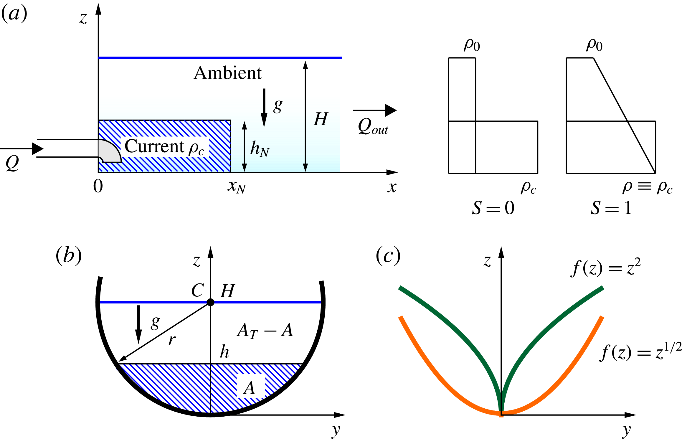
. The channel is occupied by an ambient fluid, either homogeneous or non-homogeneous; see figure 1. We introduce the thickness of the current
 $h(x,t)$
(the position of the interface between intruding and ambient fluid) and its average velocity
 $u(x,t)$
over its area
 $A$
. In many cases of interest, the intruding current, of characteristic thickness
 $h_{N}$
, is thin with respect to the thickness
 $H$
of the ambient fluid, and the density differences between the current and the ambient (of densities
 $\unicode[STIX]{x1D70C}_{c}$
and
 $\unicode[STIX]{x1D70C}_{a}$
respectively) are relatively small. We also assume that the typical width of the current is not significantly smaller than the thickness, i.e.
 $f(h_{N})\gtrsim h_{N}$
. This leads to the one-layer shallow-water (SW) Boussinesq model, incorporating two main simplifications in the high-Reynolds-number equations of motion. First, the ambient fluid is taken to be at rest (
 $u_{a}=0$
), neglecting the ‘return’ flow in the ambient above the current. This is tantamount to assuming
 $h/H\rightarrow 0$
. However, for the calculation of
 $Fr$
(the Froude-number jump condition) at the nose, a finite ratio
 $h_{N}/H$
is adopted. The second assumption is that the density difference
 $\unicode[STIX]{x1D70C}_{c}-\unicode[STIX]{x1D70C}_{a}$
is neglected in the inertia terms, but taken into account into the term driving the motion, which includes the reduced gravity
 $g^{\prime }$
.
A sketch of the current advancing in a homogeneous (
 $S=0$
) or linearly stratified ambient fluid with
 $\unicode[STIX]{x1D70C}_{b}=\unicode[STIX]{x1D70C}_{c}$
(
 $S=1$
): (a) side view; (b) cross-view; (c) two power-law cross-sections
 $f(z)\propto z^{\unicode[STIX]{x1D6FC}}$
for
 $\unicode[STIX]{x1D6FC}=1/2$
and
 $\unicode[STIX]{x1D6FC}=2$
.
We incorporate in the theory an additional physical effect, the density stratification of the ambient fluid. Following Ungarish (Reference Ungarish2015), we consider the case of a linearly stratified ambient, whose density increases from
 $\unicode[STIX]{x1D70C}_{0}$
at the top,
 $z=H$
, to
 $\unicode[STIX]{x1D70C}_{b}$
at the bottom,
 $z=0$
,
 $$\begin{eqnarray}\unicode[STIX]{x1D70C}_{c}=\unicode[STIX]{x1D70C}_{0}(1+\unicode[STIX]{x1D716}\,),\quad \unicode[STIX]{x1D70C}_{a}(z)=\unicode[STIX]{x1D70C}_{0}\left[1+\unicode[STIX]{x1D716}\,S\left(1-\frac{z}{H}\right)\right],\end{eqnarray}$$
where
 $$\begin{eqnarray}\unicode[STIX]{x1D716}\,=\frac{\unicode[STIX]{x1D70C}_{c}-\unicode[STIX]{x1D70C}_{0}}{\unicode[STIX]{x1D70C}_{0}},\quad S=\frac{\unicode[STIX]{x1D70C}_{b}-\unicode[STIX]{x1D70C}_{0}}{\unicode[STIX]{x1D70C}_{c}-\unicode[STIX]{x1D70C}_{0}},\quad g^{\prime }=\unicode[STIX]{x1D716}\,g.\end{eqnarray}$$
The additional parameter
 $S\in [0,1]$
represents the magnitude of the stratification in the ambient fluid. Two limit cases are possible: when
 $S=0$
, the ambient fluid is homogeneous; when
 $S=1$
, the maximum stratification takes place and
 $\unicode[STIX]{x1D70C}_{c}=\unicode[STIX]{x1D70C}_{b}$
. (The stratified ambient sustains internal waves with frequency
 ${\mathcal{N}}=(Sg^{\prime }/H)^{1/2}$
and maximum speed
 ${\mathcal{N}}H/\unicode[STIX]{x03C0}$
in a rectangular section, and
 ${\mathcal{N}}r/(2\sqrt{2})$
in a circular section of radius
 $r$
, which are outside the scope of this paper.)
According to the thin-layer assumption, the pressure distribution in both the ambient fluid and the intruding current is hydrostatic, i.e.
 $\unicode[STIX]{x2202}p_{i}/\unicode[STIX]{x2202}z=-\unicode[STIX]{x1D70C}_{i}g$
, where
 $p_{i}$
,
 $i=a,c$
, are the relevant pressure fields. Taking into account the continuity of the pressure at the interface
 $z=h$
, one obtains
 $$\begin{eqnarray}\displaystyle & \displaystyle p_{a}(z)=-\unicode[STIX]{x1D70C}_{0}g\left[1+\unicode[STIX]{x1D716}\,S\left(1-\frac{z}{2H}\right)\right]z+C, & \displaystyle\end{eqnarray}$$
 $$\begin{eqnarray}\displaystyle & \displaystyle p_{c}(z)=-\unicode[STIX]{x1D70C}_{0}g(1+\unicode[STIX]{x1D716}\,)(z-h)+p_{a}(h), & \displaystyle\end{eqnarray}$$
where
 $C$
is a constant. Equation (2.4) yields the
 $x$
-component of the pressure gradient as
 $$\begin{eqnarray}\frac{\unicode[STIX]{x2202}p_{c}}{\unicode[STIX]{x2202}x}=g^{\prime }\unicode[STIX]{x1D70C}_{0}\left(1-S+S\frac{h}{H}\right)\frac{\unicode[STIX]{x2202}h}{\unicode[STIX]{x2202}x},\end{eqnarray}$$
which is constant over the cross-section
 $A$
of the intruding current. We now average the
 $x$
-momentum inviscid equation over
 $A$
, taking into account inertial and buoyancy terms. The former,
 $\unicode[STIX]{x1D70C}_{c}\,\text{D}u/\text{D}t$
, is unchanged with respect to the homogeneous case; the latter is given by (2.5). Within the framework of the Boussinesq approximation (
 $\unicode[STIX]{x1D70C}_{c}\approx \unicode[STIX]{x1D70C}_{0}$
), the momentum equation is then obtained as
 $$\begin{eqnarray}\frac{\displaystyle \unicode[STIX]{x2202}u}{\displaystyle \unicode[STIX]{x2202}t}+u\frac{\displaystyle \unicode[STIX]{x2202}u}{\displaystyle \unicode[STIX]{x2202}x}=-g^{\prime }\left(1-S+S\frac{h}{H}\right)\frac{\unicode[STIX]{x2202}h}{\unicode[STIX]{x2202}x}.\end{eqnarray}$$
The mass balance equation (Ungarish Reference Ungarish2015) reads as
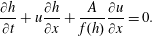 $$\begin{eqnarray}\frac{\displaystyle \unicode[STIX]{x2202}h}{\displaystyle \unicode[STIX]{x2202}t}+u\frac{\displaystyle \unicode[STIX]{x2202}h}{\displaystyle \unicode[STIX]{x2202}x}+\frac{A}{f(h)}\frac{\displaystyle \unicode[STIX]{x2202}u}{\displaystyle \unicode[STIX]{x2202}x}=0.\end{eqnarray}$$
Hereafter, we use a tilde to indicate a dimensionless variable. We scale horizontal lengths along the channel with
 $x_{0}$
, vertical lengths with
 $h_{0}$
, width with
 $f(h_{0})$
, speed with
 $U$
and time with
 $T$
, where
 $$\begin{eqnarray}U=\left(g^{\prime }h_{0}\right)^{1/2},\quad T=x_{0}/U.\end{eqnarray}$$
The scales
 $x_{0},h_{0}$
are problem-dependent. For the fixed-volume current, the length and height of the lock are appropriate. For the influx current, it is convenient to define
 $x_{0}=h_{0}=L$
, where
 $L$
is the height of the ambient
 $H$
, while for the constant-flux case, it may also be convenient to take for
 $L$
the height of the source. For the experiments discussed in this paper,
 $L=H$
.
Motivated by the analysis of the characteristics of the hyperbolic system (2.6)–(2.7), we specify the boundary condition at the nose,
 $x=x_{N}$
, as the discontinuous jump condition
 $$\begin{eqnarray}\widetilde{u}_{N}=Fr_{U}\widetilde{h}_{N}^{1/2}\unicode[STIX]{x1D6F9}^{1/2},\end{eqnarray}$$
where
 $Fr_{U}$
is the ‘Froude number’, given by (Ungarish Reference Ungarish2012)
 $$\begin{eqnarray}Fr_{U}^{2}={\displaystyle \frac{2(1-\unicode[STIX]{x1D711})}{1+\unicode[STIX]{x1D711}}}\left[1-\unicode[STIX]{x1D711}+{\displaystyle \frac{1}{hA_{T}}}\int _{0}^{h}zf(z)\text{d}z\right],\quad \unicode[STIX]{x1D711}=A/A_{T},\end{eqnarray}$$
 $A_{T}$
is the total area of the channel occupied by the fluid, and in which the stratification coefficient
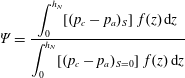 $$\begin{eqnarray}\unicode[STIX]{x1D6F9}=\frac{\displaystyle \int _{0}^{h_{N}}[(p_{c}-p_{a})_{S}]~f(z)\,\text{d}z}{\displaystyle \int _{0}^{h_{N}}[(p_{c}-p_{a})_{S=0}]~f(z)\,\text{d}z}\end{eqnarray}$$
is the ratio of pressure force over the nose with and without stratification. Using (2.3)–(2.4), we obtain
 $$\begin{eqnarray}\unicode[STIX]{x1D6F9}=1-S\left[1-\frac{1}{2}{\displaystyle \frac{h_{N}}{H}}(1+\unicode[STIX]{x1D6FE})\right],\end{eqnarray}$$
where the coefficient
 $\unicode[STIX]{x1D6FE}$
is given by
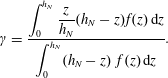 $$\begin{eqnarray}\unicode[STIX]{x1D6FE}={\displaystyle \frac{\displaystyle \int _{0}^{h_{N}}{\displaystyle \frac{z}{h_{N}}}(h_{N}-z)f(z)\,\text{d}z}{\displaystyle \int _{0}^{h_{N}}(h_{N}-z)~f(z)\,\text{d}z}}.\end{eqnarray}$$
The actual value of
 $\unicode[STIX]{x1D6FE}$
depends on the cross-section shape: for the 2-D case,
 $\unicode[STIX]{x1D6FE}=1/3$
, while for the circular cross-section,
 $\unicode[STIX]{x1D6FE}\approx 0.43$
. As regards the value of
 $\unicode[STIX]{x1D6F9}$
, it is noted that the stratification slows down the propagation: for
 $S=0$
,
 $\unicode[STIX]{x1D6F9}=1$
, then
 $\unicode[STIX]{x1D6F9}$
decreases with increasing
 $S$
.
The theoretical formulation is completed by the integral mass balance equation, expressing the injected volume
 ${\mathcal{V}}$
as
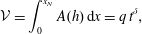 $$\begin{eqnarray}{\mathcal{V}}=\int _{0}^{x_{N}}A(h)\,\text{d}x=q\,t^{\unicode[STIX]{x1D6FF}},\end{eqnarray}$$
where
 $q>0$
,
 $\unicode[STIX]{x1D6FF}\geqslant 0$
; when the injected volume
 ${\mathcal{V}}$
is fixed and equal to
 ${\mathcal{V}}_{0}$
, then
 $\unicode[STIX]{x1D6FF}=0$
and
 $q={\mathcal{V}}_{0}$
.
For mathematical convenience, we apply the transformation
 $\unicode[STIX]{x1D709}=x/x_{N}(t)$
, which maps the
 $x\in [0,x_{N}(t)]$
domain of flow into the constant
 $\unicode[STIX]{x1D709}\in [0,1]$
(for more details, see Ungarish (Reference Ungarish2009) § 2.3). For the
 $A(\unicode[STIX]{x1D709},t),u(\unicode[STIX]{x1D709},t)$
variables, the previous equations transform according to
 $$\begin{eqnarray}\left(\frac{\unicode[STIX]{x2202}~}{\unicode[STIX]{x2202}t}\right)_{x}=\left(\frac{\unicode[STIX]{x2202}~}{\unicode[STIX]{x2202}t}\right)_{\unicode[STIX]{x1D709}}-\unicode[STIX]{x1D709}\frac{{\dot{x}}_{N}}{x_{N}}\left(\frac{\unicode[STIX]{x2202}~}{\unicode[STIX]{x2202}\unicode[STIX]{x1D709}}\right)_{t},\quad \left(\frac{\unicode[STIX]{x2202}~}{\unicode[STIX]{x2202}x}\right)_{t}=\frac{1}{\displaystyle x_{N}}\left(\frac{\unicode[STIX]{x2202}~}{\unicode[STIX]{x2202}\unicode[STIX]{x1D709}}\right)_{t},\end{eqnarray}$$
where the subscripts denote the ‘fixed’ variable in partial differentiation and the upper dot means time derivative.
After significant propagation time, the influence of the initial conditions diminishes, and the ratio
 $h_{N}/H$
is sufficiently small to justify a constant
 $Fr=Fr(0)$
approximation. We then seek a similarity solution of the form (see Zemach & Ungarish Reference Zemach and Ungarish2013; Ungarish Reference Ungarish2015)
 $$\begin{eqnarray}\widetilde{x}_{N}=K\,\widetilde{t}\,^{\unicode[STIX]{x1D6FD}_{I}},\quad \widetilde{h}(\unicode[STIX]{x1D709},\widetilde{t})=\unicode[STIX]{x1D6FA}(\widetilde{t}){\mathcal{H}}(\unicode[STIX]{x1D709}),\quad \widetilde{u}(\unicode[STIX]{x1D709},\widetilde{t})=\widetilde{{\dot{x}}}_{N}{\mathcal{U}}(\unicode[STIX]{x1D709}),\end{eqnarray}$$
where the upper dot means time derivative,
 $K,\unicode[STIX]{x1D6FD}_{I}$
are positive constants and
 $\unicode[STIX]{x1D6FA}(\widetilde{t})$
,
 ${\mathcal{H}}(\unicode[STIX]{x1D709}),\widetilde{u}(\unicode[STIX]{x1D709},\widetilde{t})$
are unknown functions. The boundary condition on the velocity is
 ${\mathcal{U}}(1)=1$
and the integral mass conservation yields
 $$\begin{eqnarray}\widetilde{{\mathcal{V}}}=\int _{0}^{\widetilde{x}_{N}}\widetilde{A}(\widetilde{h})\,\text{d}\widetilde{x}=\widetilde{x}_{N}\int _{0}^{1}\widetilde{A}[\unicode[STIX]{x1D6FA}(\widetilde{t}){\mathcal{H}}(\unicode[STIX]{x1D709})]\,\text{d}\unicode[STIX]{x1D709}=\widetilde{q}\,\widetilde{t}\,^{\unicode[STIX]{x1D6FF}},\end{eqnarray}$$
where
 $\unicode[STIX]{x1D6FF}\geqslant 0$
. The analysis proves that such a similarity solution exists only under the following restrictions (the exception is the constant-flux
 $\unicode[STIX]{x1D6FF}=1$
current). First, we must use a power-law cross-section,
 $f(z)=bz^{\unicode[STIX]{x1D6FC}}$
, where
 $b$
has dimension
 $[\text{L}^{1-\unicode[STIX]{x1D6FC}}]$
(the standard
 $f(z)=1$
included, with
 $\widetilde{{\mathcal{V}}}_{0}=1/(\unicode[STIX]{x1D6FC}+1)$
). With
 $\unicode[STIX]{x1D6FC}=1/2$
and
 $b=2\sqrt{2r}$
, this formulation captures approximately also a semicircular cross-section of radius
 $r$
. For a power-law cross-section,
 $\widetilde{A}(\widetilde{h})=\widetilde{b}\,\widetilde{h}\,^{1+\unicode[STIX]{x1D6FC}}/(1+\unicode[STIX]{x1D6FC})$
, and the integral in (2.17) attains a self-similar form. It is convenient to consider a rectangle of width
 $b$
as a power-law profile with
 $\unicode[STIX]{x1D6FC}=0$
(the formal jump of
 $f(z)$
to
 $0$
at
 $z=0$
is insignificant in our analysis). The plane case can be analysed as a rectangular case with the assumption that
 $b$
is much larger than the current depth. Second, the ambient is either homogeneous,
 $S=0$
, or has a linear density stratification under the special case of maximum stratification,
 $S=1$
. This is needed to obtain the similarity form of the
 $\widetilde{u}_{N}\equiv \widetilde{{\dot{x}}}_{N}$
condition. Under these conditions, manipulation of the momentum balance equation, the volume conservation equation and the boundary conditions at the nose yields the following results.
(i) For
 $S=0$
,
 $$\begin{eqnarray}\unicode[STIX]{x1D6FA}(\widetilde{t})=(\widetilde{{\dot{x}}}_{N})^{2},\quad {\mathcal{H}}(1)={\displaystyle \frac{1}{Fr^{2}}},\quad \unicode[STIX]{x1D6FD}_{Ih}={\displaystyle \frac{2\unicode[STIX]{x1D6FC}+2+\unicode[STIX]{x1D6FF}}{2\unicode[STIX]{x1D6FC}+3}},\end{eqnarray}$$
and the continuity and momentum equations are
 $$\begin{eqnarray}({\mathcal{U}}-\unicode[STIX]{x1D709})\frac{{\mathcal{H}}^{\prime }}{{\mathcal{H}}}+\frac{1}{\unicode[STIX]{x1D6FC}+1}{\mathcal{U}}^{\prime }=2\left(\frac{1}{\unicode[STIX]{x1D6FD}_{Ih}}-1\right),\quad {\mathcal{H}}^{\prime }+({\mathcal{U}}-\unicode[STIX]{x1D709}){\mathcal{U}}^{\prime }-\left(\frac{1}{\unicode[STIX]{x1D6FD}_{Ih}}-1\right){\mathcal{U}}=0.\end{eqnarray}$$
(ii) For
 $S=1$
,
 $$\begin{eqnarray}\unicode[STIX]{x1D6FA}(\widetilde{t})=\widetilde{{\dot{x}}}_{N},\quad {\mathcal{H}}(1)=\left(\frac{2\widetilde{H}}{1+\unicode[STIX]{x1D6FE}}\right)^{1/2}\frac{1}{\displaystyle Fr},\quad \unicode[STIX]{x1D6FD}_{Is}={\displaystyle \frac{\unicode[STIX]{x1D6FC}+1+\unicode[STIX]{x1D6FF}}{\unicode[STIX]{x1D6FC}+2}},\end{eqnarray}$$
and the continuity and momentum equations are
 $$\begin{eqnarray}({\mathcal{U}}-\unicode[STIX]{x1D709})\frac{{\mathcal{H}}^{\prime }}{{\mathcal{H}}}+\frac{1}{\unicode[STIX]{x1D6FC}+1}{\mathcal{U}}^{\prime }=\frac{1}{\unicode[STIX]{x1D6FD}_{Is}}-1,\quad \frac{1}{2\widetilde{H}}({\mathcal{H}}^{2})^{\prime }+({\mathcal{U}}-\unicode[STIX]{x1D709}){\mathcal{U}}^{\prime }-\left(\frac{1}{\unicode[STIX]{x1D6FD}_{Is}}-1\right){\mathcal{U}}=0.\end{eqnarray}$$
Here,
 $\unicode[STIX]{x1D6FD}_{Ih}$
and
 $\unicode[STIX]{x1D6FD}_{Is}$
stand for
 $\unicode[STIX]{x1D6FD}$
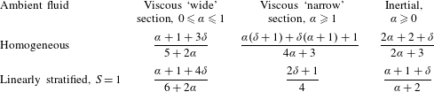
in the inertial–buoyancy regime for currents in the homogeneous (h) and stratified (s) ambient fluid respectively. These time exponents are listed later in table 1, for comparison with values obtained in the viscous regime. Letting
 $p=(\unicode[STIX]{x1D6FC}+1)(2-S)$
, (2.17) gives
 $$\begin{eqnarray}K=\left[(\unicode[STIX]{x1D6FC}+1)q\left(\unicode[STIX]{x1D6FD}_{I}^{p}\int _{0}^{1}{\mathcal{H}}^{\unicode[STIX]{x1D6FC}+1}(\unicode[STIX]{x1D709})\,\text{d}\unicode[STIX]{x1D709}\right)^{-1}\right]^{1/(1+p)}.\end{eqnarray}$$
Simple analytical solutions are obtained for two important cases,
 $\unicode[STIX]{x1D6FF}=0,1$
. First, for the fixed-volume current
 $\unicode[STIX]{x1D6FF}=0$
, we notice that the solution
 ${\mathcal{U}}=\unicode[STIX]{x1D709}$
fulfils the continuity equation, while the integration of the momentum equation produces
 ${\mathcal{H}}(\unicode[STIX]{x1D709})$
. The value of
 $K$
is then determined from (2.22). For more details, see Zemach & Ungarish (Reference Zemach and Ungarish2013) § V and Ungarish (Reference Ungarish2015) § 5 (note the rescaling (5.1) there). Second, for the constant-influx current
 $\unicode[STIX]{x1D6FF}=1$
, we find
 $\unicode[STIX]{x1D6FD}_{I}=1$
, and then notice that the slug-like propagation
 ${\mathcal{U}}=1$
and
 ${\mathcal{H}}={\mathcal{H}}(1)=1$
satisfies the continuity and momentum equation. For other values of
 $\unicode[STIX]{x1D6FF}$
, numerical solutions for
 ${\mathcal{H}},{\mathcal{U}}$
subject to the conditions at
 $\unicode[STIX]{x1D709}=1$
can be attempted.
Asymptotic self-similar solutions: values of the time scaling exponent
 $\unicode[STIX]{x1D6FD}$
of the front position,
 $\widetilde{x}_{N}\propto \widetilde{t}\,^{\unicode[STIX]{x1D6FD}}$
, for ‘narrow’ and ‘wide’ cross-sections respectively, advancing in a homogeneous (
 $S=0$
) and a linearly stratified ambient fluid with maximum stratification (
 $S=1$
).
We note that the self-similar solution for the standard 2-D (rectangular or unbounded) channel is recovered for
 $\unicode[STIX]{x1D6FC}=0$
. Here, we present a significant extension. The novelty is that self-similar currents can occur only in power-law cross-section, in particular for a rectangle,
 $\unicode[STIX]{x1D6FC}=0$
, semicircle,
 $\unicode[STIX]{x1D6FC}=1/2$
(approximately), or
 $\vee$
triangle
 $\unicode[STIX]{x1D6FC}=1$
. With hindsight, this is not surprising, because the self-similar distribution of the volume needs a compatible behaviour of the cross-section area.
In particular, for fixed-volume currents in homogeneous ambient, the rate of propagation
 $\unicode[STIX]{x1D6FD}$
increases with
 $\unicode[STIX]{x1D6FC}$
from the classical
 $2/3$
towards
 $1$
. In these cases, the transition from the slumping to the self-similar phase is less pronounced, and this may strengthen the impression of propagation with almost constant speed over a long distance.
A notable exception is the constant-flux
 $\unicode[STIX]{x1D6FF}=1$
current. In this case,
 $\unicode[STIX]{x1D6FA}=\text{const.},\unicode[STIX]{x1D6FD}_{I}=1$
, and some of the previous restrictions can be relaxed. We find that the slug-like self-similar propagation with constant
 $h_{N},u_{N}$
is an exact solution for a general
 $f(z)$
, for both Boussinesq and non-Boussinesq systems. Moreover, this solution is also valid for the two-layer model because
 $Fr$
is a constant due to the constant
 $h_{N}$
; see Longo et al. (Reference Longo, Ungarish, Di Federico, Chiapponi and Maranzoni2015b
).
The main deficiency of the similarity solutions is the vague connection with realistic initial/boundary conditions of the current. In this respect, there is no difference between the standard and the more general
 $f(z)$
cases. In particular, in the lock-released current, the shift of
 $t$
by a constant to a ‘virtual origin’ does not affect the solution.
We note that strong influx,
 $\unicode[STIX]{x1D6FF}>1$
, may cause difficulties. For
 $\unicode[STIX]{x1D6FF}>1$
, we obtain
 $\unicode[STIX]{x1D6FD}_{I}>1$
for both the
 $S=0$
and
 $1$
cases, i.e. the current accelerates. The coefficient
 $\unicode[STIX]{x1D714}=1/\unicode[STIX]{x1D6FD}_{I}-1$
, which appears in the (reduced) continuity and momentum equations, becomes negative. We thus expect a change of behaviour between
 $\unicode[STIX]{x1D6FF}<1$
and
 $\unicode[STIX]{x1D6FF}>1$
cases. This is more evident after a manipulation of the equations as follows.
The governing equations can be rewritten as follows.
(i) For
 $S=0$
,
 $$\begin{eqnarray}{\mathcal{H}}^{\prime }Q=\unicode[STIX]{x1D714}\left[{\mathcal{U}}-2(\unicode[STIX]{x1D6FC}+1)({\mathcal{U}}-\unicode[STIX]{x1D709})\right],\quad {\mathcal{U}}^{\prime }Q=\unicode[STIX]{x1D714}(\unicode[STIX]{x1D6FC}+1)\left[2-({\mathcal{U}}-\unicode[STIX]{x1D709})\frac{{\mathcal{U}}}{{\mathcal{H}}}\right],\end{eqnarray}$$
where
 $$\begin{eqnarray}Q=Q(\unicode[STIX]{x1D709})=1-(\unicode[STIX]{x1D6FC}+1)\frac{({\mathcal{U}}-\unicode[STIX]{x1D709})^{2}}{{\mathcal{H}}},\quad \unicode[STIX]{x1D714}={\displaystyle \frac{1}{\unicode[STIX]{x1D6FD}_{Ih}}}-1,\end{eqnarray}$$
with the conditions
 ${\mathcal{U}}=1,{\mathcal{H}}=1/Fr^{2},{\mathcal{U}}^{\prime }=2\unicode[STIX]{x1D714}(\unicode[STIX]{x1D6FC}+1),{\mathcal{H}}^{\prime }=\unicode[STIX]{x1D714}$
at
 $\unicode[STIX]{x1D709}=1$
. The integration is performed backwards to
 $\unicode[STIX]{x1D709}=0$
. When influx is present,
 ${\mathcal{U}}(0),{\mathcal{H}}(0)>0$
; this implies that
 $Q$
must decrease from 1 to smaller values. If
 $(1+\unicode[STIX]{x1D6FC})({\mathcal{U}}-\unicode[STIX]{x1D709})^{2}/{\mathcal{H}}=1$
at some internal point, a discontinuity of
 ${\mathcal{H}},{\mathcal{U}}$
appears. The implication is that the boundary conditions from the nose,
 $\unicode[STIX]{x1D709}=1$
, cannot influence the current for smaller values of
 $\unicode[STIX]{x1D709}$
; the influx is so strong that the conditions from the source prevail in the tail.
(ii) For
 $S=1$
, we introduce
 $$\begin{eqnarray}\unicode[STIX]{x1D705}={\mathcal{H}}/(2\widetilde{H})^{1/2},\quad Q=Q(\unicode[STIX]{x1D709})=1-(\unicode[STIX]{x1D6FC}+1)\frac{({\mathcal{U}}-\unicode[STIX]{x1D709})^{2}}{2\unicode[STIX]{x1D705}^{2}},\quad \unicode[STIX]{x1D714}={\displaystyle \frac{1}{\unicode[STIX]{x1D6FD}_{Is}}}-1.\end{eqnarray}$$
The governing equations read as
 $$\begin{eqnarray}\unicode[STIX]{x1D705}^{\prime }Q=\frac{\unicode[STIX]{x1D714}}{2\unicode[STIX]{x1D705}}\left[{\mathcal{U}}-(\unicode[STIX]{x1D6FC}+1)({\mathcal{U}}-\unicode[STIX]{x1D709})\right],\quad {\mathcal{U}}^{\prime }Q=(\unicode[STIX]{x1D6FC}+1)\unicode[STIX]{x1D714}\left[1-\frac{{\mathcal{U}}({\mathcal{U}}-\unicode[STIX]{x1D709})}{2\unicode[STIX]{x1D705}^{2}}\right],\end{eqnarray}$$
with
 ${\mathcal{U}}=1,\unicode[STIX]{x1D705}=[(1+\unicode[STIX]{x1D6FE})^{1/2}Fr]^{-1},\unicode[STIX]{x1D705}^{\prime }=\unicode[STIX]{x1D714}/2,{\mathcal{U}}^{\prime }=\unicode[STIX]{x1D714}(\unicode[STIX]{x1D6FC}+1)$
at
 $\unicode[STIX]{x1D709}=1$
. Again, we encounter the possibility of a singularity when
 $Q=0$
at some
 $\unicode[STIX]{x1D709}<1$
.
A numerical integration has been performed in order to demonstrate that the self-similar solution is an attractor; see appendix A for some results for the two critical cases with
 $S=0$
and
 $S=1$
.
3 Similarity solutions for the viscous regime
The similarity solutions discussed in the following for the viscous regime are the counterparts of those discussed in the previous section for the inertial regime and are needed to determine the critical condition. The present section recapitulates earlier results for constant-volume viscous gravity currents in a power-law
 $f(z)=bz^{\unicode[STIX]{x1D6FC}}$
cross-section filled with homogeneous ambient fluid, and derives novel scalings for more general cases including variable-volume currents and a linearly stratified ambient fluid. Typically, the current initiates the motion in an inertial (inviscid) regime, with a large Reynolds number
 $Re$
; using the lock-release
 $x_{0},h_{0}$
horizontal and vertical length scales, we define
 $Re=Uh_{0}/\unicode[STIX]{x1D708}$
, where
 $U=(g^{\prime }h_{0})^{1/2}$
. After some significant distance
 $\widetilde{x}_{V}$
(scaled with
 $x_{0}$
, the subscript
 $V$
stands for ‘viscous’), the long and thin current becomes viscous-dominated.
3.1 Current of constant volume advancing into a homogeneous ambient (
 $S=0$
)

Viscous flow in a power-law cross-section was considered by Takagi & Huppert (Reference Takagi and Huppert2007) for the special case of constant volume and homogeneous ambient fluid. The no-slip conditions on the bottom and sidewalls activate the shear
 $\unicode[STIX]{x1D708}\unicode[STIX]{x1D6FB}^{2}u$
, which balances the buoyancy driving force (per unit volume)
 $-g^{\prime }\unicode[STIX]{x2202}h/\unicode[STIX]{x2202}x$
. Therefore,
 $h$
has a negative slope, and
 $h=0$
at
 $x=x_{N}$
. The
 $z=h$
boundary of the current is a shear-free surface,
 $\unicode[STIX]{x2202}u/\unicode[STIX]{x2202}z=0$
, which represents approximately a thick layer of ambient fluid (typically, viscous effects become relevant when the intruding current is very thin).
In the following, we scale
 $x$
with
 $x_{0}$
,
 $y$
and
 $z$
with
 $h_{0}$
, speed with
 $U=(g^{\prime }h_{0})^{1/2}$
and time with
 $x_{0}/U$
;
 $b$
is scaled with
 $h_{0}^{1-\unicode[STIX]{x1D6FC}}$
and the volume with
 $x_{0}h_{0}^{2}$
.
In dimensionless form, the governing balances for momentum and continuity are
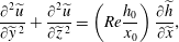 $$\begin{eqnarray}\displaystyle & \displaystyle \frac{\unicode[STIX]{x2202}^{2}\widetilde{u}}{\unicode[STIX]{x2202}\widetilde{y}\,^{2}}+\frac{\unicode[STIX]{x2202}^{2}\widetilde{u}}{\unicode[STIX]{x2202}\widetilde{z}\,^{2}}=\left(Re{\displaystyle \frac{h_{0}}{x_{0}}}\right)\frac{\unicode[STIX]{x2202}\widetilde{h}}{\unicode[STIX]{x2202}\widetilde{x}}, & \displaystyle\end{eqnarray}$$
 $$\begin{eqnarray}\displaystyle & \displaystyle f(\widetilde{h}){\displaystyle \frac{\unicode[STIX]{x2202}\widetilde{h}}{\unicode[STIX]{x2202}\widetilde{t}}}+{\displaystyle \frac{\unicode[STIX]{x2202}\widetilde{A}\widetilde{\bar{u}}}{\unicode[STIX]{x2202}\widetilde{x}}}=0,\quad \int _{0}^{\widetilde{x}_{N}}\widetilde{A}(\widetilde{x},\widetilde{t})\text{d}\widetilde{x}={\displaystyle \frac{\widetilde{b}}{\unicode[STIX]{x1D6FC}+1}}, & \displaystyle\end{eqnarray}$$
where
 $\widetilde{\bar{u}}(\widetilde{x},\widetilde{t})$
is the average of
 $\widetilde{u}(\widetilde{x},\widetilde{y},\widetilde{z},\widetilde{t})$
over the area
 $\widetilde{A}$
. The challenge is to find
 $\widetilde{u}$
that satisfies (3.1) and the abovementioned boundary conditions; it should be noted, however, that the right-hand side of (3.1) is a function of
 $\widetilde{x},\widetilde{t}$
.
For propagation and interface, we seek a self-similar solution of the type
 $$\begin{eqnarray}\widetilde{x}_{N}=K_{V}\,\widetilde{t}^{\unicode[STIX]{x1D6FD}_{Vh}},\quad \widetilde{h}=(\widetilde{x}_{N})^{-1/(\unicode[STIX]{x1D6FC}+1)}\,{\mathcal{H}}(\unicode[STIX]{x1D709}),\quad \widetilde{\bar{u}}=\unicode[STIX]{x1D6FD}_{Vh}K_{V}\widetilde{t}^{\unicode[STIX]{x1D6FD}_{Vh}-1}{\mathcal{U}}(\unicode[STIX]{x1D709}),\end{eqnarray}$$
with
 $\unicode[STIX]{x1D709}=x/x_{N}\in [0,1]$
. Here, the subscript
 $V$
means viscous, to distinguish from the self-similar solution for the inertial (inviscid) flow considered in § 2, and
 $h$
stands for ‘homogeneous’.
Takagi & Huppert (Reference Takagi and Huppert2007) obtained analytical solutions for V-shaped and semicircular sections,
 $\unicode[STIX]{x1D6FC}=1,1/2$
).
For the generic power-law cross-section, approximations in the spirit of the box model, or order-of-magnitude arguments, are useful and are reported in the following. The ratio of gap to height,
 $bh^{\unicode[STIX]{x1D6FC}-1}$
, depends strongly on
 $\unicode[STIX]{x1D6FC}$
when
 $h\rightarrow 0$
. Therefore, we distinguish between the cases.
(i) In the ‘wide’ section,
 $\unicode[STIX]{x1D6FC}<1$
, the
 $z$
shear (second term in (3.1)) is dominant; (ii) in the ‘narrow’ section,
 $\unicode[STIX]{x1D6FC}>1$
, the
 $y$
shear is dominant. Therefore, (3.1) yields the following order-of-magnitude balances:
 $$\begin{eqnarray}\displaystyle \widetilde{\bar{u}}\sim -\left(Re{\displaystyle \frac{h_{0}}{x_{0}}}\right)\widetilde{h}\,^{2}\frac{\unicode[STIX]{x2202}\widetilde{h}}{\unicode[STIX]{x2202}\widetilde{x}}\sim \left(Re{\displaystyle \frac{h_{0}}{x_{0}}}\right){\displaystyle \frac{\widetilde{h}\,^{3}}{\widetilde{x}_{N}}}\quad (\unicode[STIX]{x1D6FC}<1), & & \displaystyle\end{eqnarray}$$
 $$\begin{eqnarray}\displaystyle \widetilde{\bar{u}}\sim -\left(Re{\displaystyle \frac{h_{0}}{x_{0}}}\right)\frac{\unicode[STIX]{x2202}\widetilde{h}}{\unicode[STIX]{x2202}\widetilde{x}}\sim \left(Re{\displaystyle \frac{h_{0}}{x_{0}}}\right){\displaystyle \frac{\widetilde{h}^{2\unicode[STIX]{x1D6FC}+1}}{\widetilde{x}_{N}}}\quad (\unicode[STIX]{x1D6FC}>1). & & \displaystyle\end{eqnarray}$$
Using (3.3) (with
 ${\mathcal{H}}=1$
and
 ${\mathcal{U}}=1$
for definiteness), we find that these balances produce
 $$\begin{eqnarray}\unicode[STIX]{x1D6FD}_{Vh}=\frac{\unicode[STIX]{x1D6FC}+1}{2\unicode[STIX]{x1D6FC}+5}\quad \text{for}~\unicode[STIX]{x1D6FC}\leqslant 1,\quad \unicode[STIX]{x1D6FD}_{Vh}=\frac{\unicode[STIX]{x1D6FC}+1}{4\unicode[STIX]{x1D6FC}+3}\quad \text{for}~\unicode[STIX]{x1D6FC}\geqslant 1,\end{eqnarray}$$
and for any
 $\unicode[STIX]{x1D6FC}\geqslant 0$
,
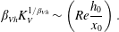 $$\begin{eqnarray}\unicode[STIX]{x1D6FD}_{Vh}K_{V}^{1/\unicode[STIX]{x1D6FD}_{Vh}}\sim \left(Re{\displaystyle \frac{h_{0}}{x_{0}}}\right).\end{eqnarray}$$
In general, since
 $\widetilde{h}=\widetilde{h}_{N}=0$
at
 $\widetilde{x}_{N}$
, the height function must display the singular behaviour
 ${\mathcal{H}}(\unicode[STIX]{x1D709})=c(1-\unicode[STIX]{x1D709})^{p}$
for
 $\unicode[STIX]{x1D709}\rightarrow 1$
. The value of
 $p$
is determined by the condition that
 $\widetilde{u}_{N}>0$
in (3.4)–(3.5); we obtain
 $p=1/3,1/(2\unicode[STIX]{x1D6FC}+1)$
for
 $\unicode[STIX]{x1D6FC}\leqslant 1$
and
 $\unicode[STIX]{x1D6FC}>1$
respectively.
A comparison of the rigorous solutions of Takagi & Huppert (Reference Takagi and Huppert2007) for a
 $\vee$
triangle and semicircle (
 $\unicode[STIX]{x1D6FC}=1,1/2$
) with the above approximate derivation shows full agreement concerning
 $\unicode[STIX]{x1D6FD}_{Vh}$
and
 $p$
, and fair agreement for
 $K_{V}$
.
For
 $\unicode[STIX]{x1D6FC}=0$
(wide rectangle,
 $b>1$
), we obtain the standard value
 $\unicode[STIX]{x1D6FD}_{Vh}=1/5$
, which turns out to be the smallest value. For
 $\unicode[STIX]{x1D6FC}=1$
(triangle), we obtain the largest value
 $\unicode[STIX]{x1D6FD}_{Vh}=2/7$
.
3.2 Current of variable volume advancing into a homogeneous
$(S=0)$
or linearly stratified ambient
$(S=1)$


The derivations of
 $\unicode[STIX]{x1D6FD}_{Vh}$
and
 $\widetilde{x}_{V}$
in § 3.1 can be extended to currents of volume
 ${\mathcal{V}}=qt^{\unicode[STIX]{x1D6FF}}$
. We start with changes in (3.2b
) (replace right-hand side with
 $\widetilde{q}\,\widetilde{t}\,^{\unicode[STIX]{x1D6FF}}$
) and (3.3b
) (replace
 $\widetilde{x}_{N}$
with
 $\widetilde{x}_{N}/(\widetilde{q}\,\widetilde{t}^{\unicode[STIX]{x1D6FF}})$
). The details are not pursued here.
We first consider a ‘wide’ cross-section (
 $\unicode[STIX]{x1D6FC}\leqslant 1$
) and a homogeneous ambient fluid,
 $S=0$
. Let
 $$\begin{eqnarray}\widetilde{x}_{N}=K_{V}\widetilde{t}^{\unicode[STIX]{x1D6FD}_{Vh}},\quad \widetilde{h}=\left({\displaystyle \frac{\widetilde{q}\,\widetilde{t}^{\unicode[STIX]{x1D6FF}}}{\widetilde{x}_{N}}}\right)^{1/(\unicode[STIX]{x1D6FC}+1)}\,{\mathcal{H}}(\unicode[STIX]{x1D709}),\quad \widetilde{\bar{u}}=\unicode[STIX]{x1D6FD}_{Vh}K_{V}\widetilde{t}^{\unicode[STIX]{x1D6FD}_{Vh}-1}{\mathcal{U}}(\unicode[STIX]{x1D709}).\end{eqnarray}$$
Substitution into (3.4) yields for
 $\unicode[STIX]{x1D6FC}\leqslant 1$
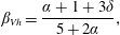 $$\begin{eqnarray}\displaystyle & \displaystyle \unicode[STIX]{x1D6FD}_{Vh}=\frac{\unicode[STIX]{x1D6FC}+1+3\unicode[STIX]{x1D6FF}}{5+2\unicode[STIX]{x1D6FC}}, & \displaystyle\end{eqnarray}$$
 $$\begin{eqnarray}\displaystyle & \displaystyle K_{V}\sim \left(Re{\displaystyle \frac{h_{0}}{x_{0}}}\right)^{(\unicode[STIX]{x1D6FC}+1)/(2\unicode[STIX]{x1D6FC}+5)}\widetilde{q}^{3/(2\unicode[STIX]{x1D6FC}+5)}. & \displaystyle\end{eqnarray}$$
For a current advancing in a linearly stratified ambient fluid with
 $S=1$
, the time exponent in the viscous regime for ‘wide’ cross-sections is similarly derived as
 $$\begin{eqnarray}\unicode[STIX]{x1D6FD}_{Vs}={\displaystyle \frac{\unicode[STIX]{x1D6FC}+1+4\unicode[STIX]{x1D6FF}}{6+2\unicode[STIX]{x1D6FC}}}\quad \text{for}\,\unicode[STIX]{x1D6FC}\leqslant 1.\end{eqnarray}$$
Similar scalings are derived for ‘narrow’ cross-sections (
 $\unicode[STIX]{x1D6FC}\geqslant 1$
) in both the homogeneous (
 $S=0$
) and linearly stratified (
 $S=1$
) cases. The relevant exponents
 $\unicode[STIX]{x1D6FD}_{Vh}$
and
 $\unicode[STIX]{x1D6FD}_{Vs}$
are reported in table 1, which includes also the scalings obtained in § 2 for inertial flows.
4 Transition length
Next, we proceed to the evaluation of
 $\widetilde{x}_{V}$
where transition between inertial and viscous regimes occurs. We observe that the typical transition is between self-similar propagation of the form
 $\widetilde{x}_{N}(\widetilde{t})=K_{j}\widetilde{t}^{\unicode[STIX]{x1D6FD}_{jh}}$
, with
 $j=V$
for viscous flow and
 $j=I$
for inertial flow. We argue that the transition is smooth, and hence at this occurrence both regimes display the same speed
 $\unicode[STIX]{x1D6FD}_{jh}K_{j}\widetilde{t}\,^{\unicode[STIX]{x1D6FD}_{jh}-1}$
and the same length
 $\widetilde{x}_{V}$
. Elimination of
 $\widetilde{t}=(\widetilde{x}_{N}/K_{j})^{1/\unicode[STIX]{x1D6FD}_{jh}}$
yields, after some algebra,
 $$\begin{eqnarray}\widetilde{x}_{Vh}=\left({\displaystyle \frac{\unicode[STIX]{x1D6FD}_{Vh}K_{V}^{1/\unicode[STIX]{x1D6FD}_{Vh}}}{\unicode[STIX]{x1D6FD}_{Ih}K_{I}^{1/\unicode[STIX]{x1D6FD}_{Ih}}}}\right)^{\unicode[STIX]{x1D706}},\quad \unicode[STIX]{x1D706}=\frac{\unicode[STIX]{x1D6FD}_{Ih}\unicode[STIX]{x1D6FD}_{Vh}}{\unicode[STIX]{x1D6FD}_{Ih}-\unicode[STIX]{x1D6FD}_{Vh}}.\end{eqnarray}$$
The values of
 $K_{I}$
and
 $\unicode[STIX]{x1D6FD}_{I}h$
for the inertial regime are available (see § 2);
 $\unicode[STIX]{x1D6FD}_{Vh}$
is given by (3.6). Precise values of
 $K_{V}$
are available for some cases (
 $\unicode[STIX]{x1D6FC}=0,1/2,1$
), and in general the approximation (3.7) can be used. The general result is
 $$\begin{eqnarray}\widetilde{x}_{Vh}=c\left(Re{\displaystyle \frac{h_{0}}{x_{0}}}\right)^{\unicode[STIX]{x1D706}},\quad \unicode[STIX]{x1D706}=\frac{\unicode[STIX]{x1D6FD}_{Ih}\unicode[STIX]{x1D6FD}_{Vh}}{\unicode[STIX]{x1D6FD}_{Ih}-\unicode[STIX]{x1D6FD}_{Vh}},\end{eqnarray}$$
where
 $c$
is of order unity (the precise value depends on
 $K_{V}$
and can be calculated for
 $\unicode[STIX]{x1D6FC}=0,1/2,1$
). The result (4.2) can be extended to a linearly stratified ambient fluid and
 $S=1$
. The value of the exponent
 $\unicode[STIX]{x1D706}$
can be evaluated from the time exponents
 $\unicode[STIX]{x1D6FD}_{Ih}$
,
 $\unicode[STIX]{x1D6FD}_{Is}$
,
 $\unicode[STIX]{x1D6FD}_{Vh}$
and
 $\unicode[STIX]{x1D6FD}_{Vs}$
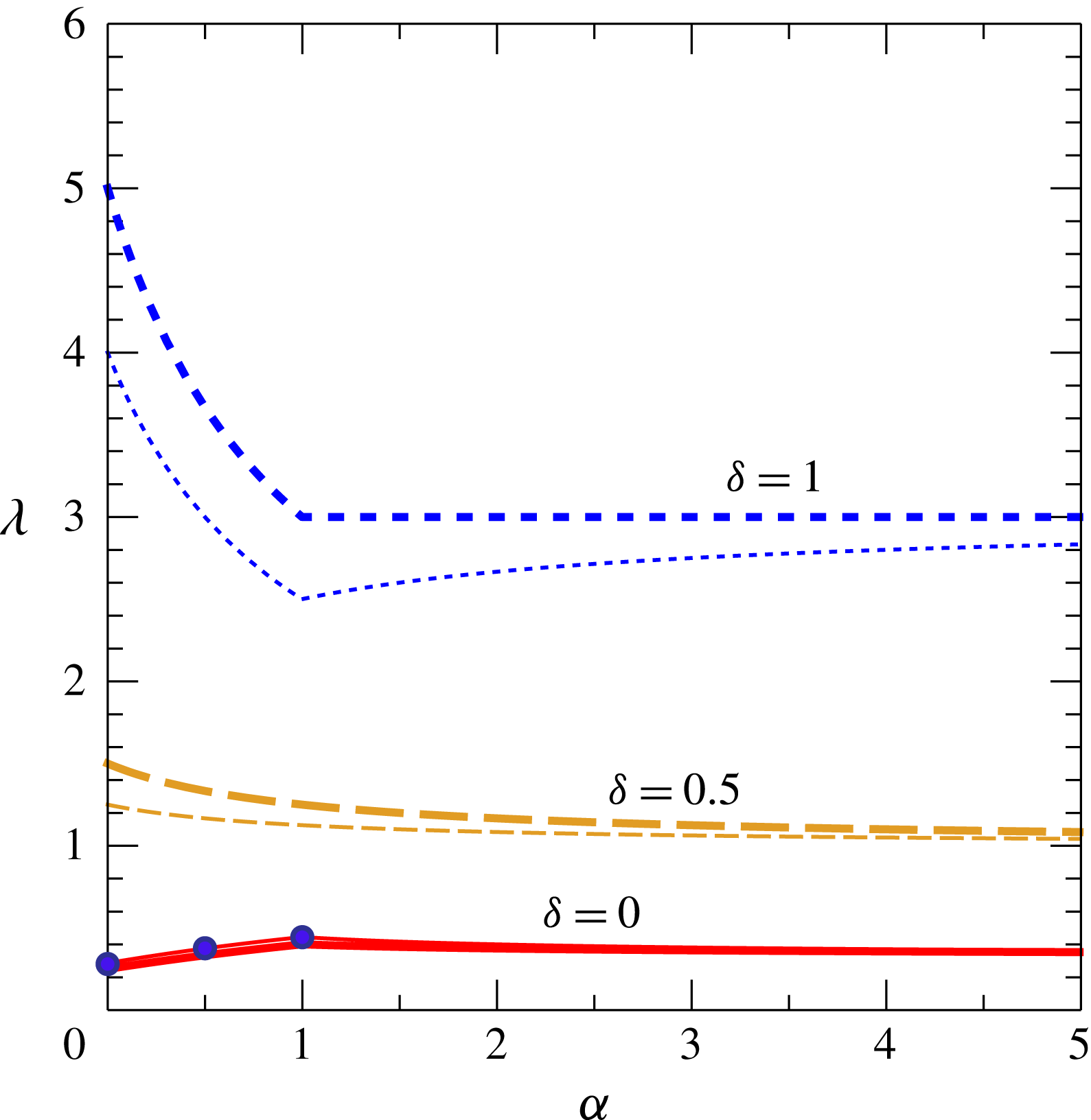
reported in table 1. Figure 2 shows the exponent
 $\unicode[STIX]{x1D706}$
for homogeneous (thin lines) and linearly stratified (thick lines) ambient fluid, for three different values of
 $\unicode[STIX]{x1D6FF}$
. We obtained a significant generalization of the standard transition-length formula (see Ungarish Reference Ungarish2009 § 2.7):
 $\widetilde{x}_{V}$
(scaled with
 $x_{0}$
of the lock) depends on
 $(Reh_{0}/x_{0})$
at some power
 $\unicode[STIX]{x1D706}\in [0.29,0.44]$
for a variety of geometries of the cross-section. The shortest transition for lock release is for the standard wide rectangle,
 $\unicode[STIX]{x1D706}=2/7\approx 0.29$
; the longest is for the
 $\vee$
triangle,
 $\unicode[STIX]{x1D706}=4/9\approx 0.44$
. For the semicircle,
 $\unicode[STIX]{x1D706}=3/8=0.375$
. For lock release in a linearly stratified ambient fluid with
 $S=1$
, the exponent is smaller with respect to the corresponding case in homogeneous ambient fluid, being
 $\unicode[STIX]{x1D706}=2/9\approx 0.22$
for the rectangle,
 $\unicode[STIX]{x1D706}=3/10=0.3$
for the semicircle and
 $\unicode[STIX]{x1D706}=4/11\approx 0.36$
for the
 $\vee$
triangle.
The power
 $\unicode[STIX]{x1D706}$
for
 $x_{V}\sim (Re(h_{0}/x_{0}))^{\unicode[STIX]{x1D706}}$
versus
 $\unicode[STIX]{x1D6FC}$
for homogeneous ambient fluid (
 $S=0$
) for lock release,
 $\unicode[STIX]{x1D6FF}=0$
(continuous thin line), waning,
 $\unicode[STIX]{x1D6FF}=0.5$
(dashed thin line), and constant influx,
 $\unicode[STIX]{x1D6FF}=1$
(dotted thin line). The symbols refer to the rectangular (
 $\unicode[STIX]{x1D706}=2/7$
), semicircular (
 $\unicode[STIX]{x1D706}=3/8$
) and triangular (
 $\unicode[STIX]{x1D706}=4/9$
) cross-sections. The thick lines refer to a linearly stratified ambient fluid with maximum stratification (
 $S=1$
).
We must keep in mind, however, that (4.2) is just an estimate. Transition between regimes occurs over a distance rather than at a certain
 $\widetilde{x}_{V}$
, and a careful calculation of the coefficient
 $c$
in (4.2) is needed for rigour.
The
 $\widetilde{x}_{V}$
estimate was subjected to laboratory tests for a triangle by Ungarish, Mériaux & Kurz-Besson (Reference Ungarish, Mériaux and Kurz-Besson2014) (see figure 6 there), and for a semicircle by Longo et al. (Reference Longo, Ungarish, Di Federico, Chiapponi and Maranzoni2015b
) (see figure 19 there). In general, the theoretical equation (4.2) underpredicts the measured
 $\widetilde{x}_{V}$
. However, there is flexibility in the definition of the experimental
 $\widetilde{x}_{V}$
, and hence more comparisons are needed for a sharper conclusion.
5 Critical regime
In this section, we consider gravity currents with volume given by
 $qt^{\unicode[STIX]{x1D6FF}}$
under a critical regime: at some critical
 $\unicode[STIX]{x1D6FF}_{c}$
, dependent of
 $\unicode[STIX]{x1D6FC}$
(channel shape), we obtain
 $\unicode[STIX]{x1D6FD}_{Vh}=\unicode[STIX]{x1D6FD}_{Ih}=\unicode[STIX]{x1D6FD}_{c}$
, and the regime (inertial or viscous) is preserved during propagation (it should be noted that, in this case,
 $\unicode[STIX]{x1D706}=0$
and
 $x_{Vh}=\infty$
; see (4.2)). This behaviour for the standard 2-D current is well documented (see Ungarish Reference Ungarish2009 § 4.2.3), but the extension to other
 $f(z)=bz^{\unicode[STIX]{x1D6FC}}$
cases is as of yet unavailable.
5.1 Homogeneous ambient fluid,
$S=0$
, ‘wide’ section

We first consider a current propagating in a homogeneous ambient fluid,
 $S=0$
. For small
 $\unicode[STIX]{x1D6FF}$
, we expect that the viscous
 $\unicode[STIX]{x1D6FD}_{Vh}$
will be smaller than the inviscid
 $\unicode[STIX]{x1D6FD}_{Ih}$
, and for some critical
 $\unicode[STIX]{x1D6FF}_{c}$
, we expect
 $\unicode[STIX]{x1D6FD}_{Ih}=\unicode[STIX]{x1D6FD}_{Vh}$
. Let us estimate the critical point for a geometry
 $bz^{\unicode[STIX]{x1D6FC}}$
,
 $\unicode[STIX]{x1D6FC}\leqslant 1$
.
We consider the viscous current, as described in § 3. Let
 $$\begin{eqnarray}\widetilde{x}_{N}=K_{V}\widetilde{t}^{\unicode[STIX]{x1D6FD}_{Vh}},\quad \widetilde{h}=\left({\displaystyle \frac{\widetilde{q}\,\widetilde{t}^{\unicode[STIX]{x1D6FF}}}{\widetilde{x}_{N}}}\right)^{1/(\unicode[STIX]{x1D6FC}+1)}\,{\mathcal{H}}(\unicode[STIX]{x1D709}),\quad \widetilde{\bar{u}}=\unicode[STIX]{x1D6FD}_{Vh}K_{V}\widetilde{t}^{\unicode[STIX]{x1D6FD}_{Vh}-1}{\mathcal{U}}(\unicode[STIX]{x1D709}).\end{eqnarray}$$
Substitution into (3.4) yields
 $$\begin{eqnarray}\displaystyle \unicode[STIX]{x1D6FD}_{Vh}=\frac{\unicode[STIX]{x1D6FC}+1+3\unicode[STIX]{x1D6FF}}{5+2\unicode[STIX]{x1D6FC}}\quad \text{for}~\unicode[STIX]{x1D6FC}\leqslant 1, & & \displaystyle\end{eqnarray}$$
 $$\begin{eqnarray}\displaystyle K_{V}\sim \left(Re{\displaystyle \frac{h_{0}}{x_{0}}}\right)^{(\unicode[STIX]{x1D6FC}+1)/(2\unicode[STIX]{x1D6FC}+5)}q^{3/(2\unicode[STIX]{x1D6FC}+5)}. & & \displaystyle\end{eqnarray}$$
For the inviscid current, we use (2.18). Then,
 $\unicode[STIX]{x1D6FD}_{Ih}=\unicode[STIX]{x1D6FD}_{Vh}$
yields the critical values
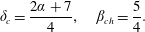 $$\begin{eqnarray}\unicode[STIX]{x1D6FF}_{c}=\frac{2\unicode[STIX]{x1D6FC}+7}{4},\quad \unicode[STIX]{x1D6FD}_{ch}=\frac{5}{4}.\end{eqnarray}$$
The 2-D rectangular counterpart corresponds to
 $\unicode[STIX]{x1D6FC}=0$
. The results agree with Ungarish (Reference Ungarish2009) § 4.2.3 (note the different notation). Interestingly,
 $\unicode[STIX]{x1D6FD}_{ch}$
does not depend on the geometry. For the semicircle
 $\unicode[STIX]{x1D6FC}=1/2$
, we obtain
 $\unicode[STIX]{x1D6FF}_{c}=2$
.
5.2 Linearly stratified ambient fluid and
$S=1$
, ‘wide’ section

For a current advancing in a linearly stratified ambient fluid and with
 $S=1$
, the time exponents in the inertial and viscous regimes are reported in table 1. Again, the condition
 $\unicode[STIX]{x1D6FD}_{Is}=\unicode[STIX]{x1D6FD}_{Vs}$
yields the critical value
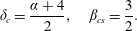 $$\begin{eqnarray}\unicode[STIX]{x1D6FF}_{c}={\displaystyle \frac{\unicode[STIX]{x1D6FC}+4}{2}},\quad \unicode[STIX]{x1D6FD}_{cs}={\displaystyle \frac{3}{2}}.\end{eqnarray}$$
As for the homogeneous ambient fluid,
 $\unicode[STIX]{x1D6FD}_{cs}$
does not depend on the shape of the cross-section. For the semicircle
 $\unicode[STIX]{x1D6FC}=1/2$
, we obtain
 $\unicode[STIX]{x1D6FF}_{c}=9/4$
.
5.3 Generalization to ‘narrow’ sections
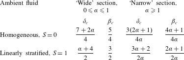
The extension to a ‘narrow’ power-law cross-section is straightforward. Table 2 lists the theoretical values of
 $\unicode[STIX]{x1D6FF}_{c}$
and
 $\unicode[STIX]{x1D6FD}_{c}$
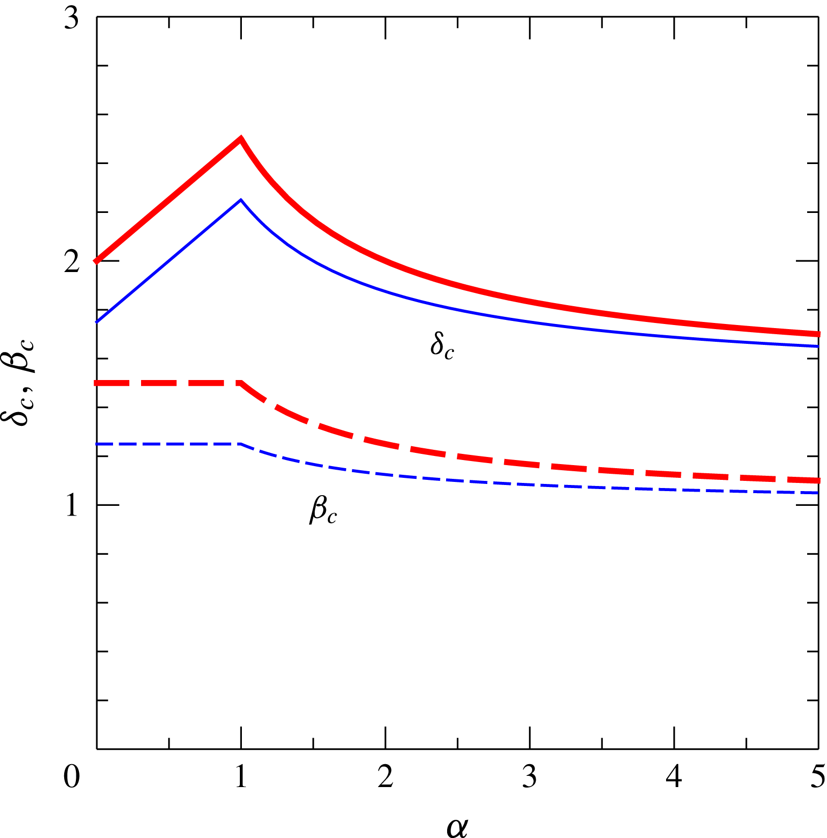
, also depicted in figure 3. The critical condition always requires a waxing current (
 $\unicode[STIX]{x1D6FF}>1$
), with a maximum value
 $\unicode[STIX]{x1D6FF}$
for a
 $\vee$
triangular cross-section (
 $\unicode[STIX]{x1D6FC}=1$
) and with
 $\unicode[STIX]{x1D6FF}_{c}\rightarrow 3/2$
for increasing
 $\unicode[STIX]{x1D6FC}$
(very ‘narrow’ sections). The current is always accelerating (
 $\unicode[STIX]{x1D6FD}_{c}>1$
); as
 $\unicode[STIX]{x1D6FC}\rightarrow \infty$
,
 $\unicode[STIX]{x1D6FD}_{c}\rightarrow 1$
, i.e. the critical current in a very narrow fracture has a constant front speed. The values of the critical parameters
 $\unicode[STIX]{x1D6FF}_{c}$
and
 $\unicode[STIX]{x1D6FD}_{c}$
are larger for a stratified than for a homogeneous ambient fluid. The impact of stratification on the critical parameters is more pronounced for ‘wide’ than for ‘narrow’ sections. The transition between
 $\unicode[STIX]{x1D6FC}<1$
and
 $\unicode[STIX]{x1D6FC}>1$
is sharp only in the present algebraic analysis which considers as dominant the shear stress in the horizontal (narrow section) or in the vertical plane (wide section), and is expected to be smooth in a more detailed study that includes the real distribution of the shear stress.
Critical values of
 $\unicode[STIX]{x1D6FF}$
and
 $\unicode[STIX]{x1D6FD}$
as functions of the shape parameter
 $\unicode[STIX]{x1D6FC}$
. The thin lines refer to the homogeneous ambient fluid and the thick lines refer to a linearly stratified ambient fluid with maximum stratification (
 $S=1$
).
Critical values of
 $\unicode[STIX]{x1D6FF}$
and
 $\unicode[STIX]{x1D6FD}$
for ‘wide’ and ‘narrow’ cross-sections and for a homogeneous (
 $S=0$
) and a linearly stratified ambient fluid (
 $S=1$
).
5.4 Scaling of the front position
In critical conditions, the front position scales with time with the same exponent
 $\unicode[STIX]{x1D6FD}\equiv \unicode[STIX]{x1D6FD}_{c}$
for both the viscous–buoyancy and inertial–buoyancy regimes; as a consequence, observation of the asymptotic
 $t^{\unicode[STIX]{x1D6FD}}$
behaviour of the current cannot identify the regime. Hence, we focus on the effect of
 $q$
as the parameter that appears in the coefficient
 $K$
of the front position, that most frequently varies in real system and that can be easily changed during the experiments. Detailed computations of the scaling of the front position with
 $q$
are given in appendices B–E for a semicircular cross-section (
 $\unicode[STIX]{x1D6FC}=1/2$
). In this case, when the ambient fluid is homogeneous (
 $S=0$
), then
 $\unicode[STIX]{x1D6FD}_{Ih}=\unicode[STIX]{x1D6FD}_{Vh}\equiv \unicode[STIX]{x1D6FD}_{ch}=5/4$
,
 $\unicode[STIX]{x1D6FF}\equiv \unicode[STIX]{x1D6FF}_{c}=2$
, and the front position at a given time is
 $\propto q^{1/2}$
in the viscous–buoyancy regime and
 $\propto q^{1/4}$
in the inertial–buoyancy regime (for a rectangular cross-section, Maxworthy (Reference Maxworthy1983) found
 $3/5=0.6$
and
 $1/3\approx 0.33$
respectively). For
 $S=1$
, then
 $\unicode[STIX]{x1D6FD}_{Is}=\unicode[STIX]{x1D6FD}_{Vs}\equiv \unicode[STIX]{x1D6FD}_{cs}=3/2$
,
 $\unicode[STIX]{x1D6FF}\equiv \unicode[STIX]{x1D6FF}_{c}=9/4$
and the front position at a given time is
 $\propto q^{4/7}$
in viscous–buoyancy balance and
 $\propto q^{2/5}$
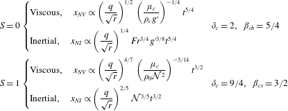
in inertial–buoyancy balance respectively. The resulting expressions are summarized in table 3 and are useful to interpret the experimental tests of § 6.
Extension of the analysis to a generic power-law cross-section
 $f(z)=bz^{\unicode[STIX]{x1D6FC}}$
gives the following for the inertial–buoyancy scaling.
For
 $S=0$
,
 $$\begin{eqnarray}K_{Ih}=\left[{\displaystyle \frac{(\unicode[STIX]{x1D6FC}+1)q}{b}}\right]^{1/(3+2\unicode[STIX]{x1D6FC})}\left({\displaystyle \frac{Fr\sqrt{g^{\prime }}}{\unicode[STIX]{x1D6FD}_{ch}}}\right)^{(2+2\unicode[STIX]{x1D6FC})/(3+2\unicode[STIX]{x1D6FC})}.\end{eqnarray}$$
For
 $S=1$
,
 $$\begin{eqnarray}K_{Is}=\left[{\displaystyle \frac{(\unicode[STIX]{x1D6FC}+1)q}{b}}\right]^{1/(2+\unicode[STIX]{x1D6FC})}\left({\displaystyle \frac{Fr{\mathcal{N}}}{\unicode[STIX]{x1D6FD}_{cs}\sqrt{2}}}\right)^{(1+\unicode[STIX]{x1D6FC})/(2+\unicode[STIX]{x1D6FC})}.\end{eqnarray}$$
The length of the current (dimensional) in a semicircular cross-section, for the viscous–buoyancy and inertial–buoyancy regimes in critical conditions, for
 $S=0$
(homogeneous ambient fluid) and
 $S=1$
(linearly stratified ambient fluid with a maximum stratification).
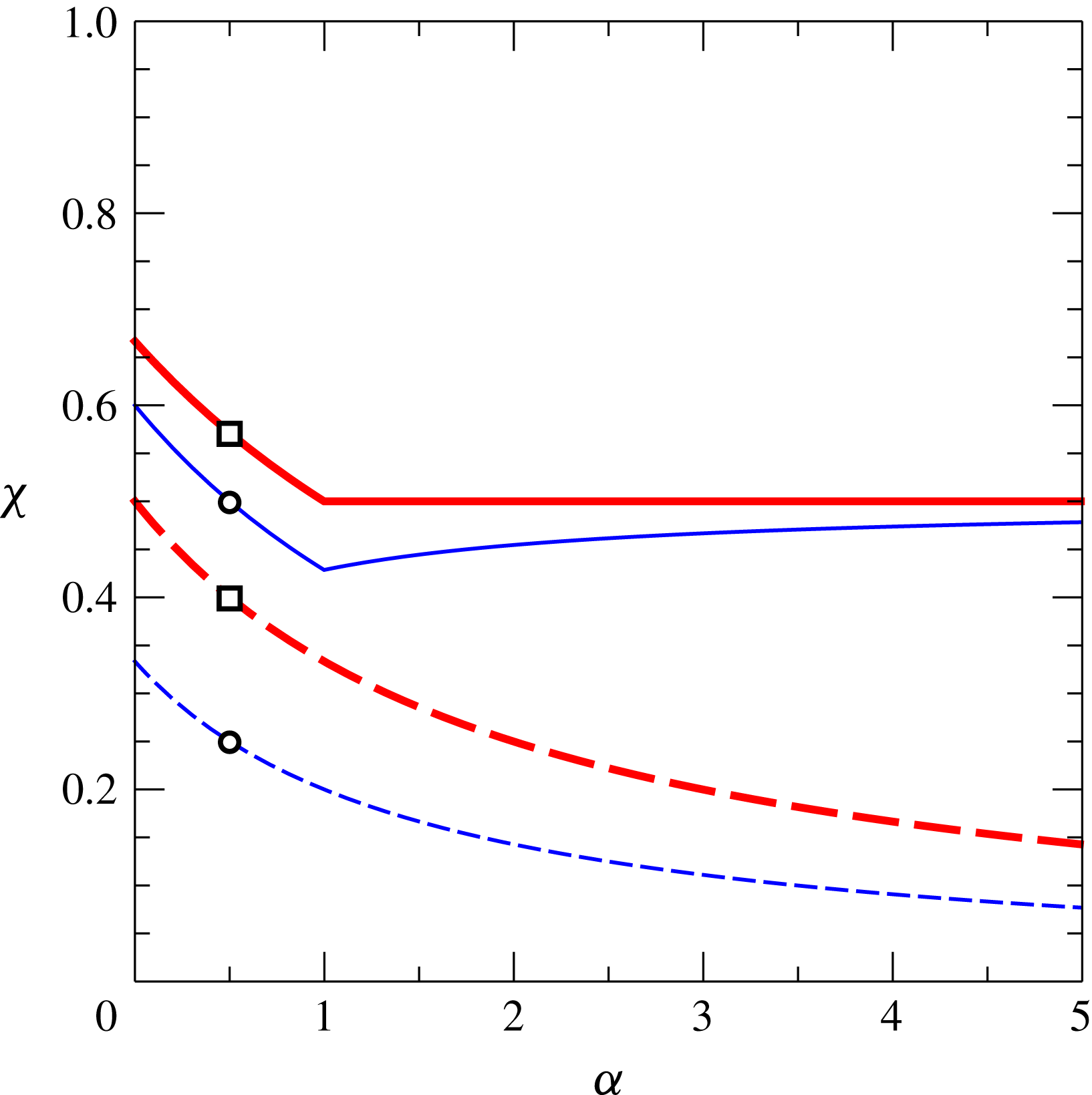
A generalization of the dependence of
 $x_{N}\propto q^{\unicode[STIX]{x1D712}}$
for different cross-sections is listed in table 4 and shown in figure 4. The exponent
 $\unicode[STIX]{x1D712}$
is larger in the viscous–buoyancy than in the inertial–buoyancy regime, and the difference increases with
 $\unicode[STIX]{x1D6FC}$
and is almost constant for ‘wide’ sections. The theoretical difference of
 $\unicode[STIX]{x1D712}$
is sufficiently large for suggesting that this is a good criterion for accurate identification of the regime of propagation in experiments with critical conditions and various
 $q$
. This prediction is tested and confirmed in § 6.
The dependence of the front position
 $x_{N}$
on
 $q$
in critical conditions,
 $x_{N}\propto q^{\unicode[STIX]{x1D712}}$
, for
 $S=0$
in the viscous (thin continuous line) and inertial (thin dashed line) regimes, and for
 $S=1$
in the viscous (thick continuous line) and inertial (thick dashed line) regimes. The symbols indicate the values of
 $\unicode[STIX]{x1D712}$
for the present experiments in a semicircular cross-section (
 $\unicode[STIX]{x1D6FC}=1/2$
) with homogeneous (circles) and stratified (squares) ambient fluid.
5.5 Estimate of the regime in critical condition
We have established that a proper way to experimentally detect the regime (viscous–buoyancy or inertial–buoyancy) of a current in critical condition is to perform experiments with different values of
 $q$
(all the other parameters are kept constant) and to observe the dependence of the front position on
 $q$
.
The dependence of the front position on
 $q$
for ‘wide’ and ‘narrow’ cross-sections.

In order to estimate the balance, we first consider a semicircular cross-section and the case
 $S=0$
, with
 ${\mathcal{V}}=qt^{2}$
and
 $\unicode[STIX]{x1D6FD}_{ch}=5/4$
. The effective ratio between inertial and viscous forces is
 $$\begin{eqnarray}Re_{e}={\displaystyle \frac{u_{N}h_{N}^{2}}{\unicode[STIX]{x1D708}x_{N}}}.\end{eqnarray}$$
By using the inertial branch and the box-model approximation with
 $h=h_{N}$
,
 $x_{N}=Kt^{\unicode[STIX]{x1D6FD}_{ch}}\rightarrow u_{N}=\unicode[STIX]{x1D6FD}x_{N}/t$
,
 ${\dot{x}}_{N}=u_{N}=Fr\sqrt{g^{\prime }h_{N}}$
,
 $A=(4/3)\sqrt{2r}h^{3/2}$
,
 ${\mathcal{V}}=Ax_{N}$
, all in dimensional form, substitution into (5.8) yields
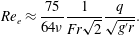 $$\begin{eqnarray}Re_{e}\approx {\displaystyle \frac{75}{64\unicode[STIX]{x1D708}}}{\displaystyle \frac{1}{Fr\sqrt{2}}}{\displaystyle \frac{q}{\sqrt{g^{\prime }r}}}.\end{eqnarray}$$
The balance is viscous–buoyancy if
 $Re_{e}$
is below a threshold value of order unity; otherwise it is inertial–buoyancy. For constant
 $\unicode[STIX]{x1D708}$
,
 $r$
, the inertia/viscous forces ratio behaves like
 $q/\sqrt{g^{\prime }}$
.
Along the same lines, the effective Reynolds number for a current in a semicircular cross-section with
 $S=1$
, with
 ${\mathcal{V}}=qt^{9/4}$
and
 $\unicode[STIX]{x1D6FD}_{cs}=3/2$
, is
 $$\begin{eqnarray}Re_{e}\approx {\displaystyle \frac{3}{2\unicode[STIX]{x1D708}}}{\displaystyle \frac{1}{(1+\unicode[STIX]{x1D6FE})^{2/5}}}\left({\displaystyle \frac{9}{8Fr}}\right)^{4/5}\left({\displaystyle \frac{q}{{\mathcal{N}}\sqrt{r}}}\right)^{4/5}.\end{eqnarray}$$
We can generalize the estimate of
 $Re_{e}$
for a cross-section
 $f(z)=bz^{\unicode[STIX]{x1D6FC}},~\unicode[STIX]{x1D6FC}\leqslant 1$
(
 $bh^{\unicode[STIX]{x1D6FC}}$
is the width, equal to
 $2\sqrt{2rh}$
for the approximated circular cross-section).
For
 $S=0$
, let
 $l=4/(2\unicode[STIX]{x1D6FC}+3)$
(also equal to
 $1/(\unicode[STIX]{x1D6FF}_{ch}-1)$
),
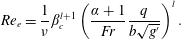 $$\begin{eqnarray}Re_{e}=\frac{1}{\displaystyle \unicode[STIX]{x1D708}}\unicode[STIX]{x1D6FD}_{c}^{l+1}\left(\frac{\unicode[STIX]{x1D6FC}+1}{Fr}\frac{q}{b\sqrt{g^{\prime }}}\right)^{l}.\end{eqnarray}$$
For
 $S=1$
, let
 $p=2/(\unicode[STIX]{x1D6FC}+2)$
(also equal to
 $1/(\unicode[STIX]{x1D6FF}_{cs}-1)$
),
 $$\begin{eqnarray}Re_{e}=\frac{1}{\displaystyle \unicode[STIX]{x1D708}}\unicode[STIX]{x1D6FD}_{c}^{~p+1}{\displaystyle \frac{1}{(1+\unicode[STIX]{x1D6FE})^{p/2}}}\left[{\displaystyle \frac{(\unicode[STIX]{x1D6FC}+1)\sqrt{2}}{Fr}}{\displaystyle \frac{q}{{\mathcal{N}}b}}\right]^{p}.\end{eqnarray}$$
In the ‘narrow’ channel,
 $\unicode[STIX]{x1D6FC}>1$
, the lateral shear is dominant and hence the effective
 $Re_{e}$
is given by
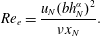 $$\begin{eqnarray}Re_{e}={\displaystyle \frac{u_{N}(bh_{N}^{\unicode[STIX]{x1D6FC}})^{2}}{\unicode[STIX]{x1D708}x_{N}}}.\end{eqnarray}$$
Using the same box-model estimates for
 $x_{N},u_{N},h_{N}$
, we obtain the following.
For
 $S=0$
, let
 $l=4\unicode[STIX]{x1D6FC}/(2\unicode[STIX]{x1D6FC}+3)$
,
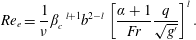 $$\begin{eqnarray}Re_{e}=\frac{1}{\displaystyle \unicode[STIX]{x1D708}}\unicode[STIX]{x1D6FD}_{c}^{~l+1}b^{2-l}\left[\frac{\unicode[STIX]{x1D6FC}+1}{Fr}\frac{q}{\sqrt{g^{\prime }}}\right]^{l}.\end{eqnarray}$$
For
 $S=1$
, let
 $p=2\unicode[STIX]{x1D6FC}/(\unicode[STIX]{x1D6FC}+2)$
,
 $$\begin{eqnarray}Re_{e}=\frac{1}{\displaystyle \unicode[STIX]{x1D708}}\unicode[STIX]{x1D6FD}_{c}^{~p+1}b^{2-p}{\displaystyle \frac{1}{(1+\unicode[STIX]{x1D6FE})^{p/2}}}\left[{\displaystyle \frac{(\unicode[STIX]{x1D6FC}+1)\sqrt{2}}{Fr}}\frac{q}{{\mathcal{N}}}\right]^{p}.\end{eqnarray}$$
For the triangle,
 $\unicode[STIX]{x1D6FC}=1$
, the ‘wide’ and ‘narrow’
 $Re_{e}$
coincide only for
 $b=1$
. This is because
 $b=$
(width/height), and hence we should use (5.8) for
 $b>1$
and (5.13) for
 $b<1$
.
The conclusion is that in the critical current system (influx with critical
 $\unicode[STIX]{x1D6FF}_{c}$
), the ratio of inertia to viscous forces is proportional to
 $q/\sqrt{g^{\prime }}$
for
 $S=0$
, and to
 $q/{\mathcal{N}}$
for
 $S=1$
. For a given current, this ratio may be large or small, but it is time-independent. The current is expected to be in the inertial regime if
 $Re_{e}$
is large and in the viscous regime if this parameter is small. It is convenient to define a threshold value
 $Re_{et}$
which separates the regimes. Some intermediary regime must exist, but the experimental work of Maxworthy (Reference Maxworthy1983) indicated that
 $Re_{et}$
is fairly sharp for a 2-D current, and we therefore expect a similar behaviour in the general case. Since both the inviscid and the viscous theories lose accuracy in the intermediate regime, the reliable value of
 $Re_{et}$
must be determined by experiments, as detailed later.
6 Experimental layout and procedures
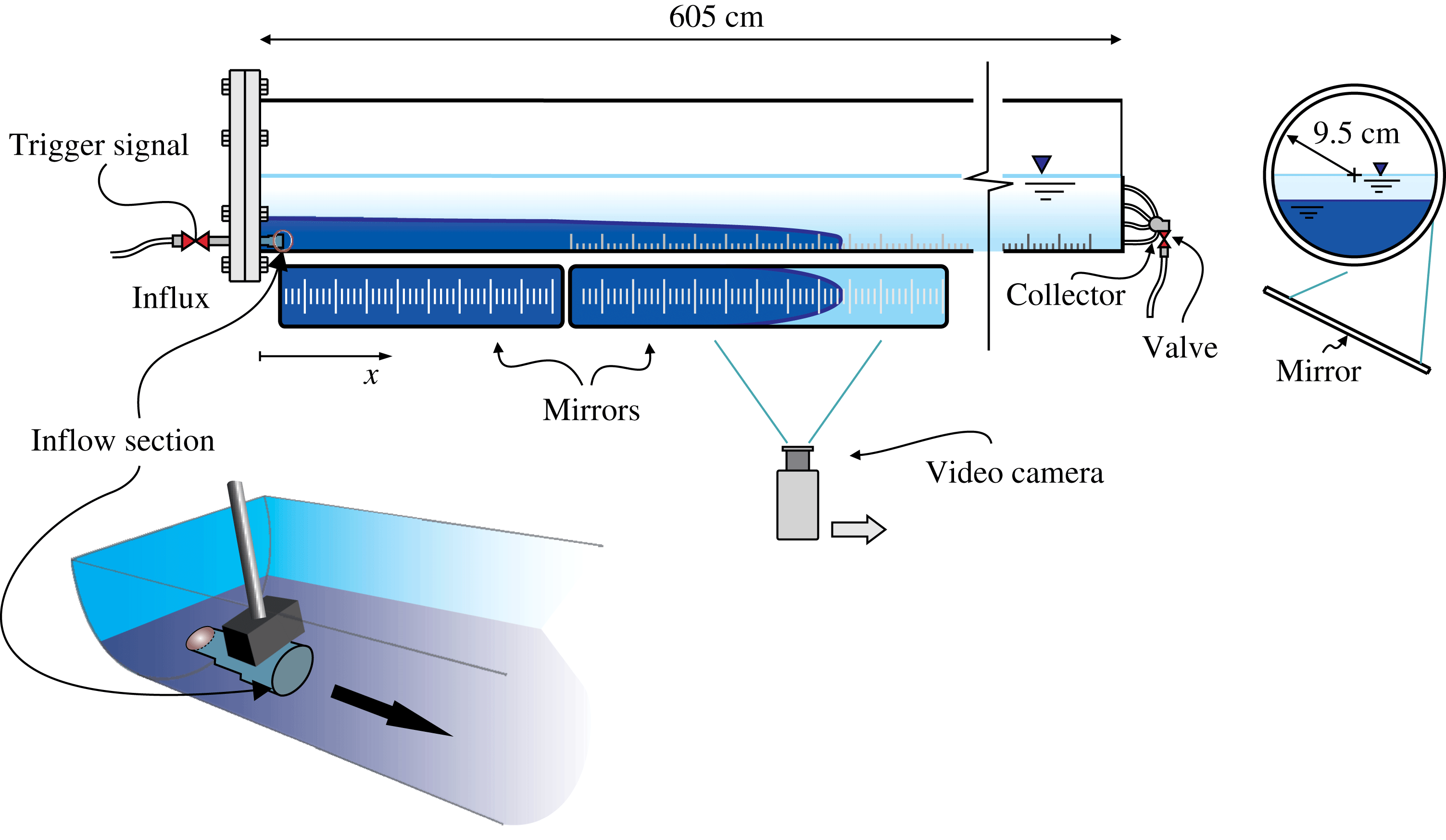
A series of experiments were planned and executed in the Hydraulic Laboratory of the University of Parma to test the validity of the models developed for a gravity current propagating into homogeneous and inhomogeneous ambient fluid in critical conditions. The experiments were conducted in a circular tube of polymethyl methacrylate (PMMA), a transparent thermoplastic, with an internal radius
 $r=9.5~\text{cm}$
and a length of
 $605~\text{cm}$
; see figure 5. The same apparatus was used by Longo et al. (Reference Longo, Ungarish, Di Federico, Chiapponi and Addona2016b
). A pipe connected to a vane pump was positioned in the inflow section. The pump was equipped with an inverter for discharge feedback control; the sensor was a turbine meter operating in the flow rate interval
 $5{-}250~\text{cm}^{3}~\text{s}^{-1}$
, with an overall accuracy equal to
 $\pm 1~\text{cm}^{3}~\text{s}^{-1}$
. The inflow rate time dependence
 $Q=\unicode[STIX]{x1D6FF}qt^{\unicode[STIX]{x1D6FF}-1}$
was imposed via software by a PC through a DAQ board. For inflow rates less than the threshold of the turbine meter, the pump was controlled without a feedback system, with a voltage signal controlling the inverter proportional to the target inflow rate, according to a calibration curve.
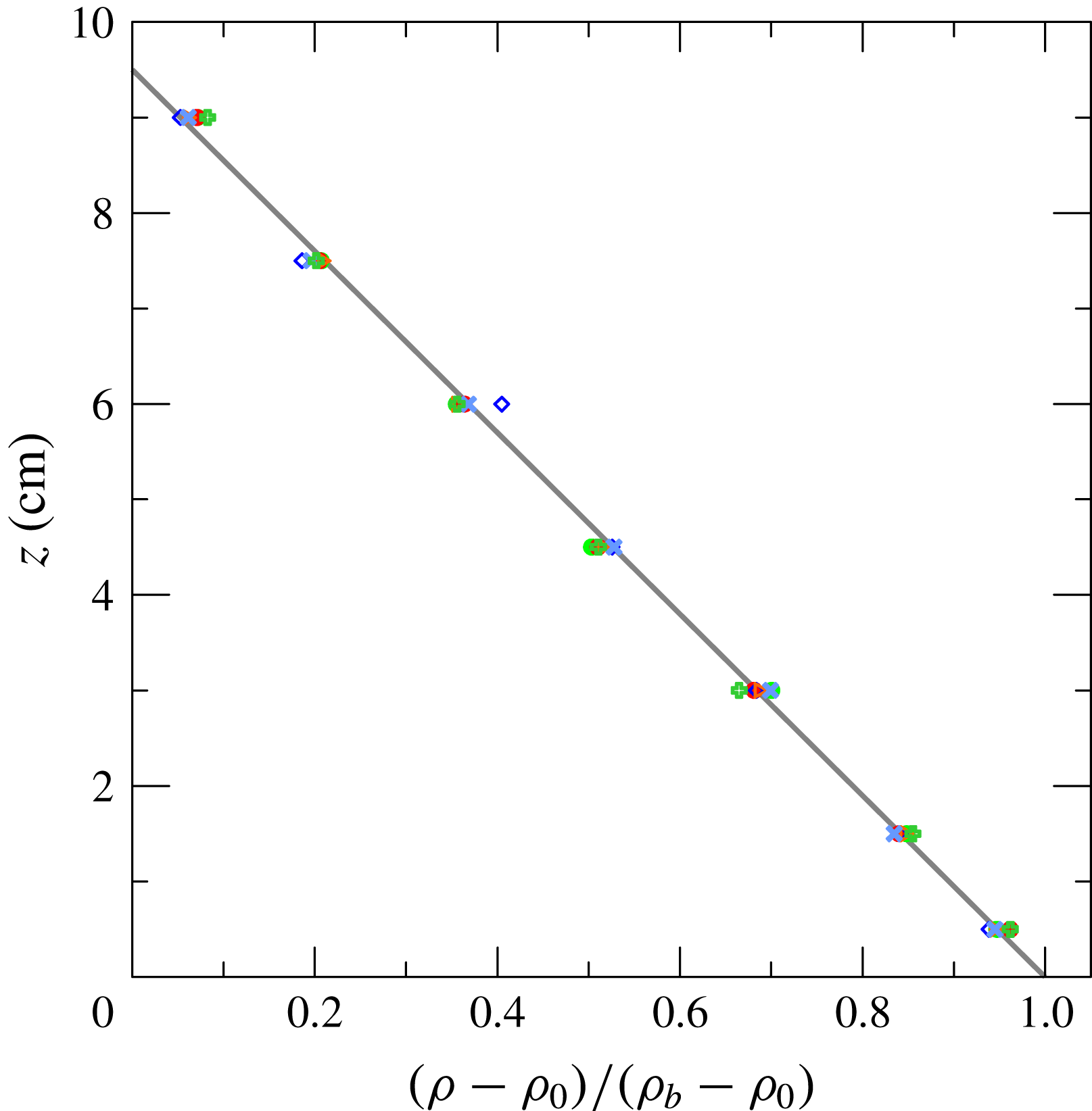
In a first series of tests, the ambient fluid was homogeneous; the second series of tests required a linearly stratified ambient fluid, which was obtained with the methodology and the devices described in Longo et al. (Reference Longo, Ungarish, Di Federico, Chiapponi and Addona2016a
). To check the density profile in the tank, a small quantity of fluid was drained at different depths in the tank with a syringe connected to a small pipe of 0.1 cm in diameter. Then, the mass density of the sample was measured by a hydrometer with an uncertainty of
 $10^{-3}~\text{g}~\text{cm}^{-3}$
. Figure 6 depicts the normalized density profiles for several experiments, which collapse on the theoretical line with a limited discrepancy.
The layout of the experimental set-up.
Density profiles measured in the tank. The symbols refer to different experiments, the straight line indicates the perfect linearity.
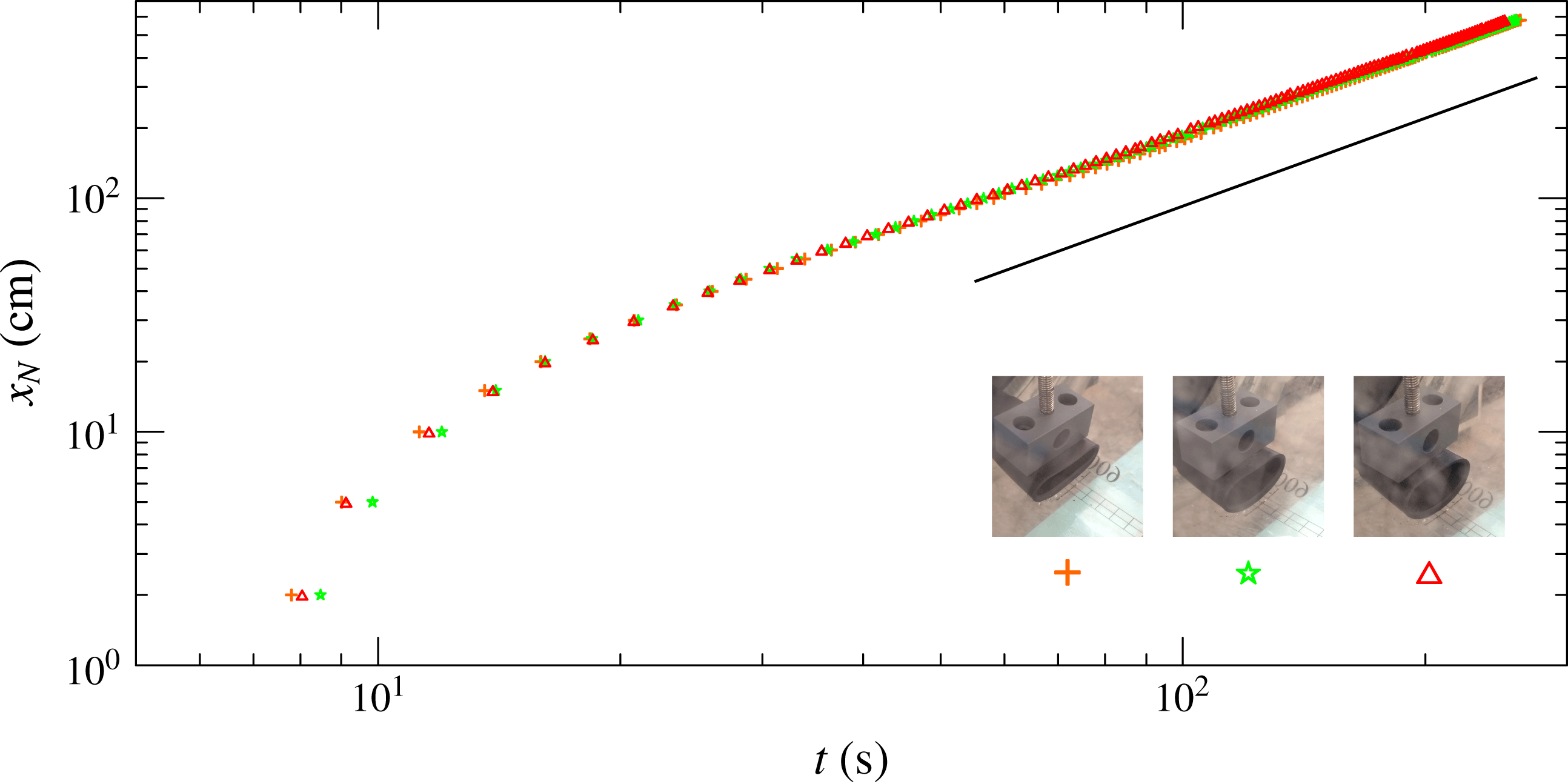
Front position for three experiments with
 $\unicode[STIX]{x1D70C}_{c}=1.060~\text{g}~\text{cm}^{-3}$
, with different inlet cross-section areas,
 $A\approx 4~\text{cm}^{2}$
(crosses),
 $A\approx 7~\text{cm}^{2}$
(stars) and
 $A\approx 9~\text{cm}^{2}$
(triangles), with
 ${\mathcal{V}}=0.2t^{2}~\text{cm}^{3}$
(
 $t$
in seconds). The continuous line represents the theoretical asymptotic self-similar solution
 $x_{N}\propto t^{5/4}$
. The currents are in the critical regime and viscous–buoyancy balance.
The position of the front of the currents was determined using a full HD video camera (Canon Legria HF 20;
 $1920\times 1080$
pixels) with a data rate of 25 frames per second; the camera was translated parallel to the pipe in order to keep the nose of the current in the field of view. A grid stuck at the bottom of the tube was used to detect the front position of the current with an overall uncertainty of less than 0.2 cm.
Since the experiments required an accurate and repeatable measurement of the front position in time (in other experiments, only the asymptotic trend of the front is required, which is much less sensitive to disturbances), special attention was devoted to obtaining uniform inlet (in order to avoid disturbances due to, e.g., different dissipation rates of the intruding current) and outlet conditions.
The inlet pipe was made of rubber which could be easily deformed in order to vary the cross-sectional area. Figure 7 shows the front position in time for three tests with
 $\unicode[STIX]{x1D70C}_{c}=1.060~\text{g}~\text{cm}^{-3}$
and with different areas of the inlet cross-section, equal to
 ${\approx}4$
, 7 and
 $9~\text{cm}^{2}$
. There are small differences among the profiles; further, while near the entrance the current with the smallest inlet section was the fastest (due to a jet-like behaviour), asymptotically the current injected from the largest inlet cross-section (
 ${\approx}9~\text{cm}^{2}$
) was slightly faster than the other two currents, as a consequence of minor dissipation. The dissipation was essentially due to the expansion of the current. Having checked that the area of the inlet pipe did not affect the shape of the
 $x_{N}(t)$
function, all of the experiments were carried out with the inlet pipe having the maximum area.
The data shown in figure 7 also indicate the extension of the disturbances due to the inlet section before approaching the self-similar regime; the length of adaptation is approximately 30 cm (say
 $3H$
). This length of adaptation depends on several factors like the discharge rate and the cross-section area of the inlet pipe with respect to the cross-section area of the ambient fluid.
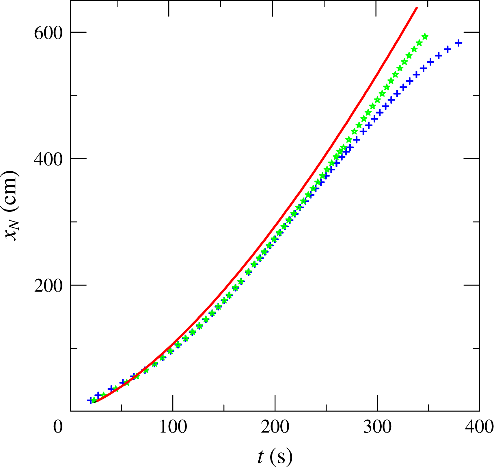
Position of the front measured for two tests in identical conditions (Exp. 37), linearly stratified ambient fluid and
 $S=1$
, critical regime (
 $\unicode[STIX]{x1D6FF}=9/4$
), with the active outflow (star symbols) and the passive outflow (plus symbols). The curve represents the theoretical self-similar solution in viscous–buoyancy balance; see appendix D, equation (D 13).
The outflow section was delimited by a weir with a crest at a fixed position in order to guarantee a depth of
 $H=9.5~\text{cm}$
during all of the tests with homogeneous ambient fluid. For the tests with density stratified ambient fluid, a drain with 12 small-diameter pipes distributed over the cross-section was inserted into the outflow section in order to avoid selective withdrawal. The pipes were connected to a valve, which was regulated during the experiment in order to keep a constant level in the channel. The efficiency and necessity of this arrangement were verified by comparing two tests conducted under identical experimental conditions, but using two different outflow systems, the weir (passive) and the control valve (active); see figure 8. A good overlap between the experimental results is evident for approximately half of the channel length; then, the effect of the accumulation of the denser fluid becomes evident, as the outflow over the crest of the weir drains only the lighter fluid. The theoretical solution, computed by assuming a viscous–buoyancy regime (see Longo et al.
Reference Longo, Di Federico and Chiapponi2015a
), is also shown in the figure. This solution overpredicts both datasets, highlighting the approximations intrinsic in the model, which in addition generally cause underestimation of the dissipation level. The choice of the minimum density of the current was mainly based on the need to guarantee an adequate accuracy in measurements and a reasonable correspondence of the experimental layout with the model, with a high signal/noise ratio. In fact, the density of the fluid can be measured with very accurate instruments; hence, it was possible to handle experiments with
 $g^{\prime }$
values of a few
 $\text{cm}~\text{s}^{-2}$
. However, it is difficult to guarantee the homogeneity of the ambient fluid in the whole channel with a level of accuracy comparable to the accuracy in measuring the density, since temperature variations or other external effects are a source of disturbances adding noise of comparable level to the signal. For this reason, we chose a minimum mass density equal to
 $1.030~\text{g}~\text{cm}^{-3}$
. The maximum density is dictated by the need to satisfy the Boussinesq approximation, with
 $\unicode[STIX]{x1D716}<10\,\%$
.
The theory assumes that the current is thin and the return flow is small. These conditions were satisfied in our experiments, with the exception of a small initial time. This was verified by visual inspection and also by calculations following the injected volume. In particular, it should be noted that in our experiments, the typical volume of the initial ambient fluid was approximately
 $0.5\unicode[STIX]{x03C0}r^{2}l_{tank}=85\,\text{l}$
, while the volume of the current
 $qt_{max}^{\unicode[STIX]{x1D6FF}}$
was approximately 2–6 l. At
 $t_{max}$
, the current was spread over the length
 $l_{tank}$
with a typical thickness of
 $1{-}2~\text{cm}$
.
6.1 Uncertainty in variables and parameters
The relative uncertainty in
 $g^{\prime }$
was
 $0.2\,\%$
and the uncertainty in the stratification parameter
 $S=(\unicode[STIX]{x1D70C}_{b}-\unicode[STIX]{x1D70C}_{0})/(\unicode[STIX]{x1D70C}_{c}-\unicode[STIX]{x1D70C}_{0})$
was
 $\unicode[STIX]{x0394}S/S=3.2\,\%$
. The level of the ambient fluid was fixed with an accuracy of 0.1 cm, inducing a relative uncertainty of
 $\unicode[STIX]{x0394}H/H\leqslant 1.1\,\%$
. The velocity scale had an uncertainty of
 $\unicode[STIX]{x0394}U/U\leqslant 0.6\,\%$
and the time scale had an uncertainty equal to
 $\unicode[STIX]{x0394}T/T\leqslant 1.7\,\%$
. The influx rate was measured with an uncertainty equal to 1 % of the instantaneous value, and the dimensionless influx rate had an uncertainty equal to
 $\unicode[STIX]{x0394}q/q\leqslant 4.3\,\%$
. By assuming an uncertainty of
 $1\,\%$
in the value of the kinematic viscosity of the denser fluid, the resulting uncertainty in the Reynolds number was
 $\unicode[STIX]{x0394}Re/Re\leqslant 2.7\,\%$
.
6.2 Experiments
Two series of experiments were performed, the first with homogeneous ambient fluid (22 experiments with varying
 $q$
and three different density values of the current) and the second with a linearly stratified ambient fluid and
 $S=1$
(nine experiments with varying
 $q$
). The main parameters of the experiments are listed in tables 5 and 6.
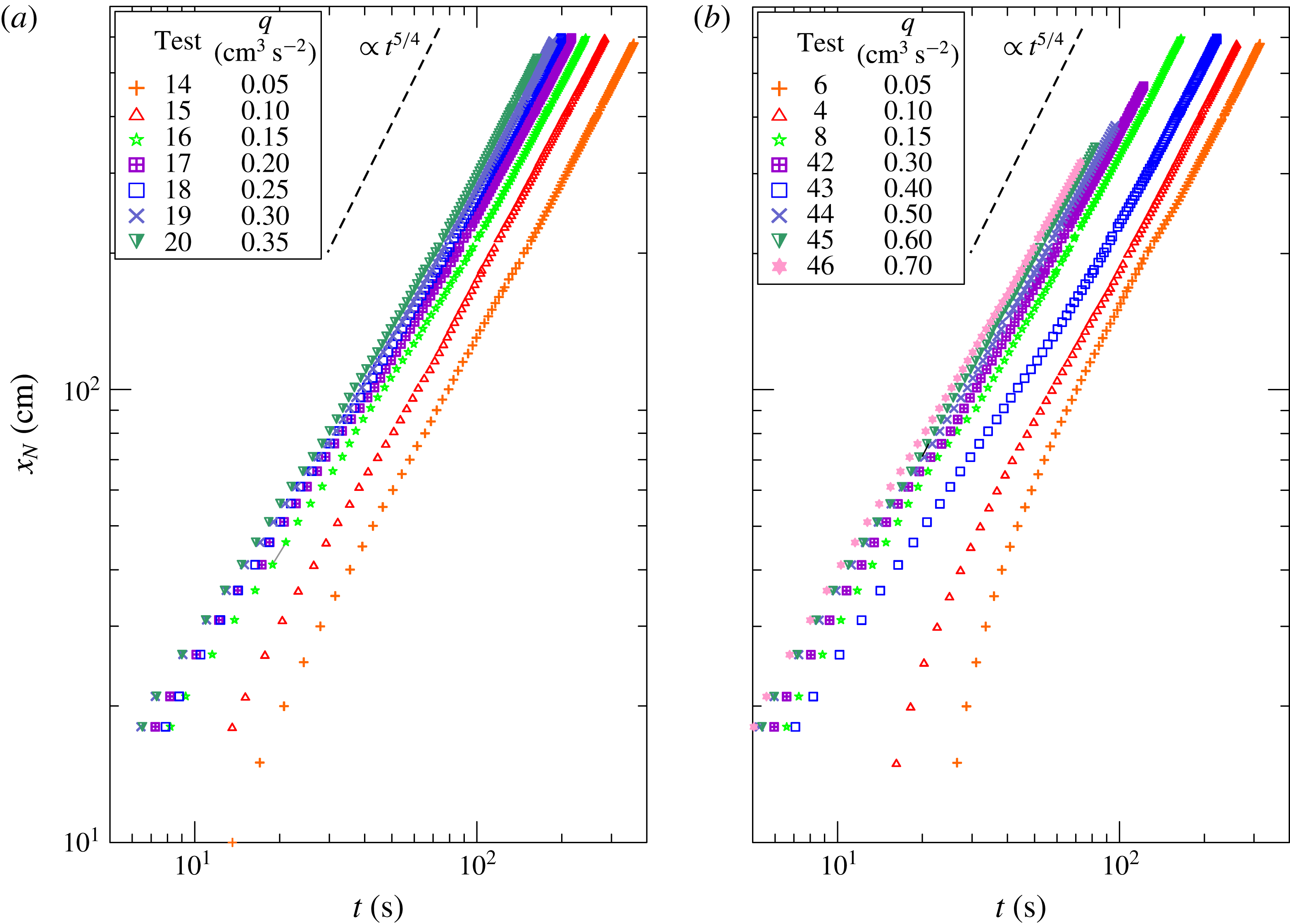
Front position for (a) seven tests with
 $\unicode[STIX]{x1D70C}_{c}=1.030~\text{g}~\text{cm}^{-3}$
and (b) eight tests with
 $\unicode[STIX]{x1D70C}_{c}=1.060~\text{g}~\text{cm}^{-3}$
, with homogeneous ambient fluid (
 $S=0$
). The straight dashed lines indicate the front position,
 $x_{N}\propto t^{5/4}$
.
Front position for (a) seven tests with
 $\unicode[STIX]{x1D70C}_{c}=1.090~\text{g}~\text{cm}^{-3}$
, with homogeneous ambient fluid (
 $S=0$
), and (b) nine tests with a linearly stratified ambient fluid,
 $\unicode[STIX]{x1D70C}_{c}=1.086~\text{g}~\text{cm}^{-3}$
,
 $S=1$
, and with data-fit curves of the equation
 $x_{N}=a+K(q)t^{\unicode[STIX]{x1D6FD}_{c}}$
. The straight dashed lines indicate the front position,
 $x_{N}\propto t^{5/4}$
and
 $x_{N}\propto t^{3/2}$
respectively.
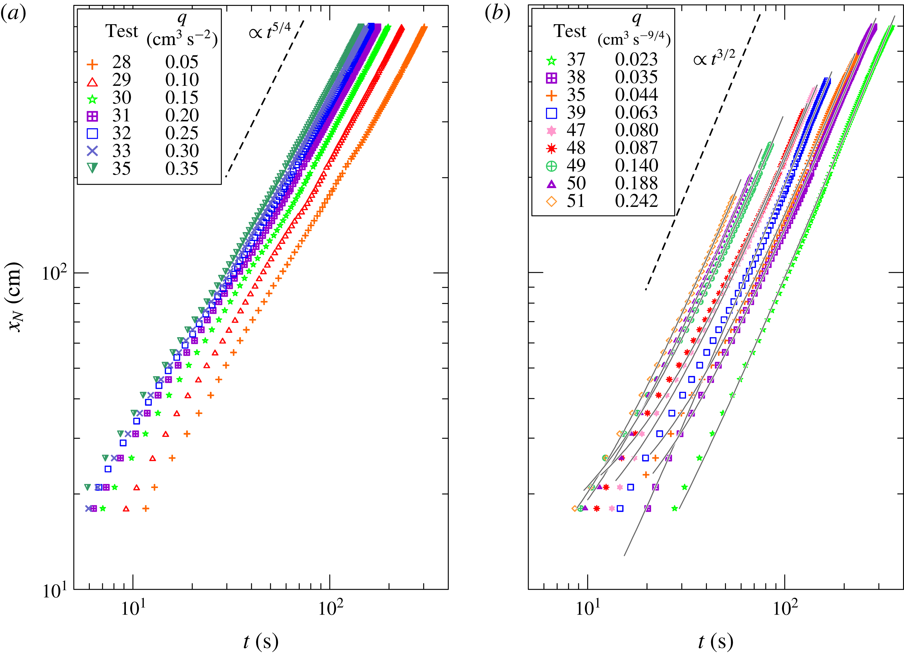
Figures 9 and 10 show the front position of the currents for the homogeneous ambient fluid and the linearly stratified ambient fluid (
 $S=1$
). The straight lines indicate the theoretical asymptotic regime of the self-similar solutions. For both datasets, there is a reasonable collapse of the data in the asymptotic limit; the experimental
 $\unicode[STIX]{x1D6FD}$
is slightly smaller than the theoretical one. The different value of
 $\unicode[STIX]{x1D6FD}$
can be attributed in general to the dissipation level, which in the experiments is invariably greater than the theoretical one. There are some other considerations. For the inertial current, in practice,
 $Fr$
is not a constant as assumed. In the critical flow,
 $h\sim t^{1/2}$
and
 $Fr$
decreases; therefore, the practical propagation is slower, with a smaller
 $\unicode[STIX]{x1D6FD}$
. In the viscous current, there is shear from the side, which we neglected. This will also hinder propagation and cause a smaller
 $\unicode[STIX]{x1D6FD}$
. We also keep in mind that the circle section is not a perfect power-law profile. This is also expected to contribute to the discrepancy between theory and experimental data.
Parameters of the experiments with homogeneous ambient fluid (
 $S=0$
). The channel is circular with radius
 $r=9.5~\text{cm}$
, half filled with ambient fluid (
 $H=9.5~\text{cm}$
). The volume is
 ${\mathcal{V}}=qt^{\unicode[STIX]{x1D6FF}}$
,
 $\unicode[STIX]{x1D716}=(\unicode[STIX]{x1D70C}_{c}-\unicode[STIX]{x1D70C}_{0})/\unicode[STIX]{x1D70C}_{0}$
,
 $g^{\prime }=g\unicode[STIX]{x1D716}$
is the reduced gravity,
 $U=\sqrt{g^{\prime }H}$
is the velocity scale,
 $T=H/U$
is the time scale,
 $Re=UH/\unicode[STIX]{x1D708}$
, where
 $\unicode[STIX]{x1D708}$
is the kinematic viscosity of the current. The terms
 $a$
and
 $K(q)$
are the coefficients of the interpolating curve
 $x_{N}=a+K(q)t^{\unicode[STIX]{x1D6FD}_{c}}$
, with uncertainty
 ${\leqslant}4\,\%$
and
 ${\leqslant}3\,\%$
on
 $a$
and
 $K(q)$
respectively;
 $Re_{e}$
is the effective Reynolds number; the balance is viscous–buoyancy (v–b) or inertial–buoyancy (i–b).
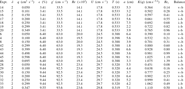
Parameters of the experiments with linearly stratified ambient fluid and
 $S=1$
. The term
 ${\mathcal{N}}$
is the buoyancy frequency. For the other symbols, see the caption to table 5.
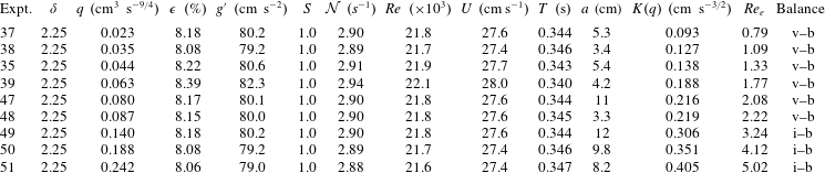
In order to detect the different regimes, we have fitted the experimental dataset for each experiment with a function
 $x_{N}=a+K(q)t^{\unicode[STIX]{x1D6FD}_{c}}$
(see figure 10(b) for an example of the data-fit lines), obtaining a series of values
 $K(q)$
, shown in figure 11 for the four series of experiments. We expect that
 $K(q)\propto q^{\unicode[STIX]{x1D712}}$
, where the theoretical
 $\unicode[STIX]{x1D712}$
is given in table 3 for the different regimes. In each series of data, it is possible to detect two branches with an exponent slightly different from the theoretical value but showing a significant variation in the two regimes. The vertical dashed lines indicate the value of
 $q$
that separates currents in a viscous–buoyancy regime (below) and currents in an inertial–buoyancy regime (above). See also tables 5 and 6, containing the indication of the balance and the effective Reynolds number.
The coefficient
 $K(q)$
of the front position
 $x_{N}=K(q)t^{\unicode[STIX]{x1D6FD}_{c}}$
. (a–c) Homogeneous ambient fluid with
 $\unicode[STIX]{x1D70C}_{c}=1.030,1.060,1.090~\text{g}~\text{cm}^{-3}$
respectively; the theoretical dependence is
 $K(q)\propto q^{1/2}$
in viscous–buoyancy balance and
 $K(q)\propto q^{1/4}$
in inertial–buoyancy balance. (d) Linearly stratified ambient fluid,
 $\unicode[STIX]{x1D70C}_{c}=1.086~\text{g}~\text{cm}^{-3}$
,
 $S=1$
; the theoretical dependence is
 $K(q)\propto q^{4/7}$
in viscous–buoyancy balance and
 $K(q)\propto q^{2/5}$
in inertial–buoyancy balance. The dashed lines limit the 95 % confidence band, and the vertical dashed lines indicate the value of
 $q$
separating the viscous–buoyancy (below) and inertial–buoyancy (above) regimes.
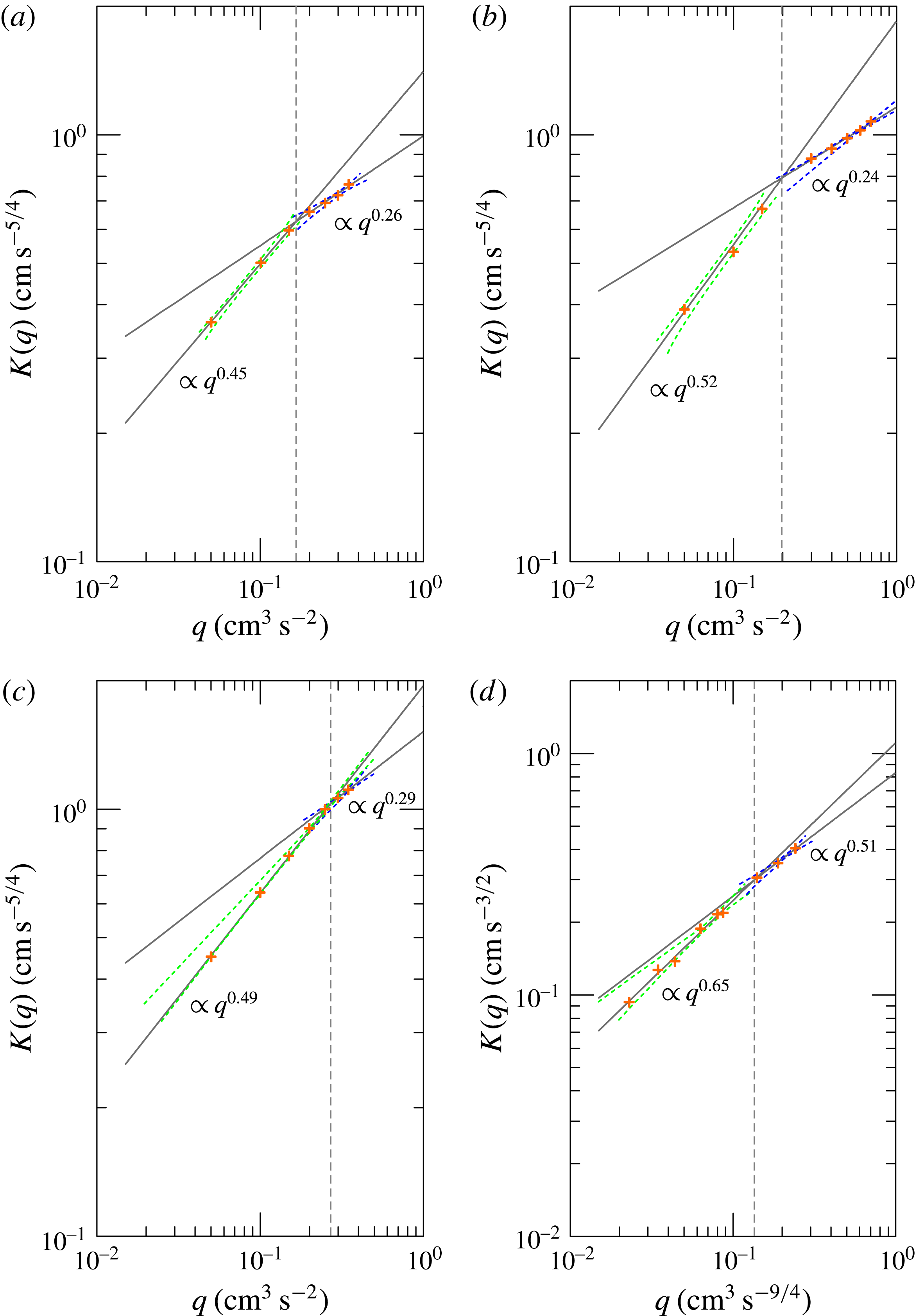
For currents advancing in a homogeneous ambient fluid, the threshold separating the two regimes has been computed using the intersection point of the data-fit functions of the lower and the upper series of experimental data in figure 11(a–c), where the intersection is observed for
 $q\approx 0.17,0.20,0.27~\text{cm}^{3}~\text{s}^{-2}$
for the experiments with
 $\unicode[STIX]{x1D70C}_{c}=1.030,1.060,1.090~\text{g}~\text{cm}^{-3}$
(
 $\unicode[STIX]{x1D716}=3.4,6.4,9.4\,\%$
).
By adopting
 $Fr=\sqrt{2}$
in (5.9), the corresponding effective Reynolds number marking the threshold is
 $Re_{et}=0.46,0.40,0.45$
for the three series, a value that is fairly constant. In comparing theory and experiments, numerous approximations inherent in the model should be kept in mind: a parabolic cross-section in lieu of a circular one, a negligible effect of the ambient fluid dynamics, use of the box model, which excludes all the details of the current shape, and the fact that regime transition is not a sharp effect. Consequently, the fact that the threshold separating the two regimes occurs at
 $Re_{e}$
approximately equal to 1 should be considered to be fair agreement with prediction. We can compare the present results for currents advancing in homogeneous ambient fluid with similar results obtained by Maxworthy (Reference Maxworthy1983) in a rectangular cross-section. For a rectangular cross-section with homogeneous ambient fluid, the effective Reynolds number is
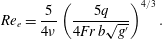 $$\begin{eqnarray}Re_{e}={\displaystyle \frac{5}{4\unicode[STIX]{x1D708}}}\left({\displaystyle \frac{5q}{4Fr\,b\sqrt{g^{\prime }}}}\right)^{4/3}.\end{eqnarray}$$
Inserting the data of the transition documented by Maxworthy (Reference Maxworthy1983) in his three sets of experiments the effective threshold Reynolds number is
 $Re_{et}=0.96,0.89,0.92$
, again of
 $O(1)$
. We remind readers that the experiments where transition takes place (Maxworthy Reference Maxworthy1983) are characterized by the following parameters:
 $J=2.9,3.5,3.4$
,
 $q/b=0.033,0.030,0.055~\text{cm}^{2}~\text{s}^{-7/4}$
,
 $g^{\prime }\equiv (\unicode[STIX]{x0394}\unicode[STIX]{x1D70C}/\unicode[STIX]{x1D70C})g=1.27,1.18,3.73~\text{cm}~\text{s}^{-2}$
,
 $\unicode[STIX]{x1D708}=0.01~\text{cm}^{2}~\text{s}^{-1}$
,
 $[(K_{I}(7/4)/K_{V}(7/4))]^{15}=2.2$
, where
 $K_{I}$
and
 $K_{V}$
are constants.
For currents advancing in a linearly stratified ambient fluid (
 $S=1$
, figure 11
d), the intersection occurs at
 $q\approx 0.13~\text{cm}^{3}~\text{s}^{-9/4}$
, with a corresponding effective threshold Reynolds number
 $Re_{et}\approx 3$
for
 $Fr=\sqrt{2}$
in (5.10).
7 Summary and conclusions
We have investigated the behaviour of critical gravity currents, advancing with both viscous–buoyancy and inertial–buoyancy regimes in a homogeneous ambient fluid (
 $S=0$
) and a linearly stratified ambient fluid with maximum stratification (
 $S=1$
). In both regimes, a self-similar solution is expected. The analysis has been detailed theoretically for a generic power-law cross-section,
 $f(z)=bz^{\unicode[STIX]{x1D6FC}}$
, and checked experimentally for a semicircular cross-section, locally approximated by a parabola (
 $\unicode[STIX]{x1D6FC}=1/2$
). It is important to keep in mind the behaviour of the current in different conditions.
-
(1) In subcritical condition (
$\unicode[STIX]{x1D6FF}<\unicode[STIX]{x1D6FF}_{c}$
), the current starts in the inertial–buoyancy regime and then at a finite time turns into the viscous–buoyancy state, with a smaller
$\unicode[STIX]{x1D6FD}$
. The value of
$Re_{e}$
is initially large and decreases with time (and
$x_{N}$
). -
(2) In supercritical condition (
$\unicode[STIX]{x1D6FF}>\unicode[STIX]{x1D6FF}_{c}$
), the current starts in the viscous–buoyancy regime and then (again at a finite time) turns into the inertial–buoyancy state, with a smaller
$\unicode[STIX]{x1D6FD}$
. The value of
$Re_{e}$
is initially small and increases with time (and
$x_{N}$
). -
(3) In critical condition, the current is in the inertial or the viscous regime from the beginning. Both regimes have the same
$\unicode[STIX]{x1D6FD}$
. The current maintains the regime (i.e.
$Re_{e}$
is constant during the propagation).


Our work leads to the following major conclusions.
-
(1) A collection of relatively simple closed-form solutions is available to describe the advancement of GCs in inertial and viscous regimes in a fairly realistic set-up including a channel of assigned shape and a stratified ambient. Self-similarity is satisfied within the experimental uncertainty.
-
(2) Specific scalings are derived for the propagation of the current in critical conditions. A stratified ambient requires a larger
$\unicode[STIX]{x1D6FF}$
and a larger acceleration to reach the critical condition as compared to a homogeneous ambient. The impact of stratification on the critical parameters is more pronounced for ‘wide’ than for ‘narrow’ sections. -
(3) A subcritical current (
$\unicode[STIX]{x1D6FF}<\unicode[STIX]{x1D6FF}_{c}$
) starts in inertial–buoyancy balance and then turns to viscous–buoyancy balance; a supercritical current (
$\unicode[STIX]{x1D6FF}>\unicode[STIX]{x1D6FF}_{c}$
) starts in viscous–buoyancy balance and then turns to inertial–buoyancy balance. -
(4) A critical current, after an initial adaptation, propagates according to the asymptotic represented by the self-similar solution for the specific regime dictated by the effective Reynolds number: viscous–buoyancy if
$Re_{e}<Re_{et}$
; inertial–buoyancy if
$Re_{e}>Re_{et}$
. However, the precise value of the effective Reynolds number separating the two regimes cannot be evaluated from our model, and must be obtained empirically. -
(5) Since the asymptotic
$x_{N}\sim t^{\unicode[STIX]{x1D6FD}}$
behaviour of the current in critical condition cannot be used to discriminate the regime (viscous–buoyancy or inertial–buoyancy), the dependence of the front position as a function of the discharge parameter
$q$
can be used for this purpose. The experimental results for a current with three different values of
$g^{\prime }$
, advancing in a homogeneous ambient fluid, show that the flow is in a viscous–buoyancy balance below a threshold value of
$q$
and is in an inertial–buoyancy balance above this value, with good agreement with theory within the uncertainties. -
(6) For a semicircle, we obtained the experimental effective threshold Reynolds number separating the two different balances,
$Re_{et}$
, is
${\approx}0.5$
for a homogeneous ambient fluid and
${\approx}3$
for a linearly stratified one, consistent with theoretical predictions of
$Re_{et}=O(1)$
. Figure 12 contains the key elements of the analysis, which has been developed for the generic cross-section and has been experimentally validated for the circular cross-section.


Diagram of the theoretical propagation-behaviour of a gravity current in a power-law channel of width
 $f(z)=bz^{\unicode[STIX]{x1D6FC}}$
with homogeneous,
 $S=0$
, or stratified,
 $S=1$
, ambient and volume
 ${\mathcal{V}}=qt^{\unicode[STIX]{x1D6FF}}$
.
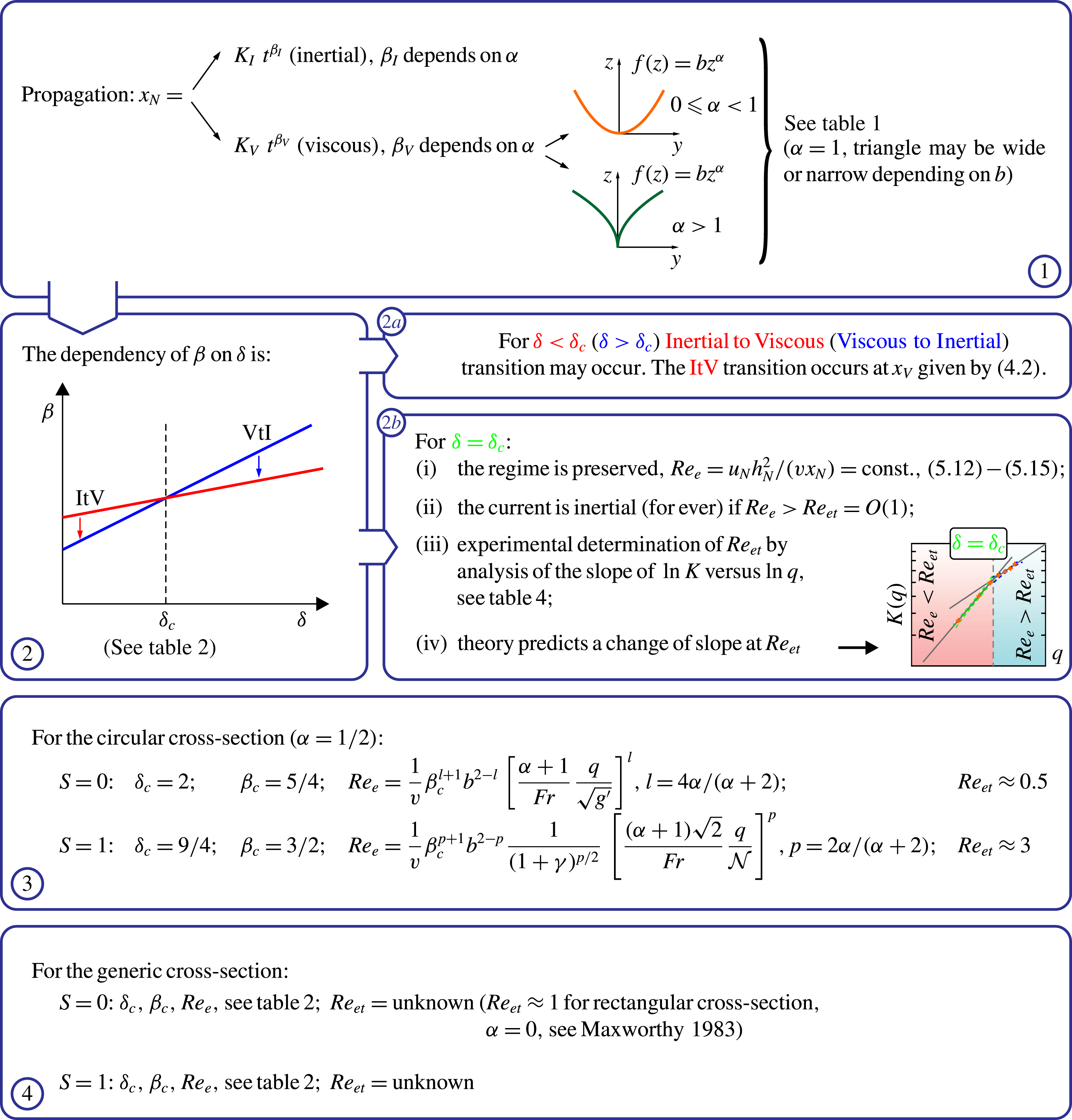
The laboratory preparations and observations provided specific insights into the mechanics of the current and suggestions about the management of the experiments, as follows.
-
(1) Preliminary tests show that the inlet conditions, varied by changing the area of the inlet pipe, have a minor effect on the propagation of the currents, whose speed is only marginally affected by the extent of the dissipation at the inlet. This loss of memory with respect to the initial and boundary conditions was already known for GCs, but had never been tested in experiments with variable inflow rate. A significant effect of ‘selective withdrawal’ was identified for GCs advancing in a linearly density stratified fluid. This effect significantly slows down the current; hence, care must be taken to avoid it in setting up the experiments.
-
(2) The experimental value of
$\unicode[STIX]{x1D6FD}$
is slightly lower than the theoretical value as a consequence of numerous effects neglected by the simple model adopted for comparison.

Future work could include a better modelling of the advancing current via a two-layer model, and more detailed experiments to check the transition length for subcritical and supercritical currents.
Acknowledgements
We thank I. Lauriola for her support during the revision of the paper.
Appendix A. Numerical verification of the asymptotic regime
In order to check that the asymptotic behaviour of the current evolves towards the self-similar solution represented by (2.16), we have integrated the equations (2.23)–(2.24) valid for homogeneous ambient fluid (
 $S=0$
) with the method of characteristics. The (time-varying) integration domain was mapped onto
 $[0,1]$
through the transforms (2.15) and then the equations written in the new domain were integrated along the two trajectories with space step and time step chosen in order to guarantee a Courant number
 ${\approx}0.5$
, usually equal to
 $1/100$
and
 $1/200$
respectively. The boundary condition at the nose is given by (2.9) and the boundary at the inlet follows the indications given in Shringarpure et al. (Reference Shringarpure, Lee, Ungarish and Balachandar2013), with a fixed inlet
 $Fr_{in}=\widetilde{u}_{in}/\sqrt{\widetilde{h}_{in}}$
, where
 $Fr_{in}$
is the inlet Froude number. The inlet velocity
 $\widetilde{u}_{in}$
and current depth
 $\widetilde{h}_{in}$
are time varying in order to satisfy the time-varying discharge and the constant inlet Froude number.
Figure 13(a) shows the front position as a result of the numerical integration for a circular cross-section and
 $\unicode[STIX]{x1D6FF}=2$
, and figure 13(b) shows the time variation of the exponent computed as
 $\unicode[STIX]{x1D6FD}=\widetilde{{\dot{x}}}_{N}\widetilde{t}/\widetilde{x}_{N}$
, which tends to assume the theoretical value
 $\unicode[STIX]{x1D6FD}\equiv \unicode[STIX]{x1D6FD}_{Ih}=5/4$
. Figure 13(c) shows the current depth at different times.
The numerical integration was also performed for the equations (2.25)–(2.26) valid for stratified ambient fluid (
 $S=1$
). Figure 14(a) shows the front position as a result of the numerical integration for a circular cross-section and
 $\unicode[STIX]{x1D6FF}=9/4$
, and figure 14(b) shows the time variation of the exponent, which tends to assume the theoretical value
 $\unicode[STIX]{x1D6FD}\equiv \unicode[STIX]{x1D6FD}_{Is}=3/2$
. Figure 14(c) shows the current depth at different times.
Numerical model results for a current advancing in a circular cross-section in the inertial–buoyancy regime in a homogeneous ambient fluid (
 $S=0$
), with volume
 $\propto t^{2}$
(
 $\unicode[STIX]{x1D6FF}=2$
). (a) The time series of the front position
 $\widetilde{x}_{N}$
(symbols) and the interpolating function of the equation
 $\widetilde{x}_{N}\propto \widetilde{t}^{1.24}$
(continuous red curve); (b) the time series of the exponent
 $\unicode[STIX]{x1D6FD}_{Ih}$
, with the dashed horizontal line representing the theoretical value
 $\unicode[STIX]{x1D6FD}_{Ih}=5/4$
; (c) profiles of the current at different times.
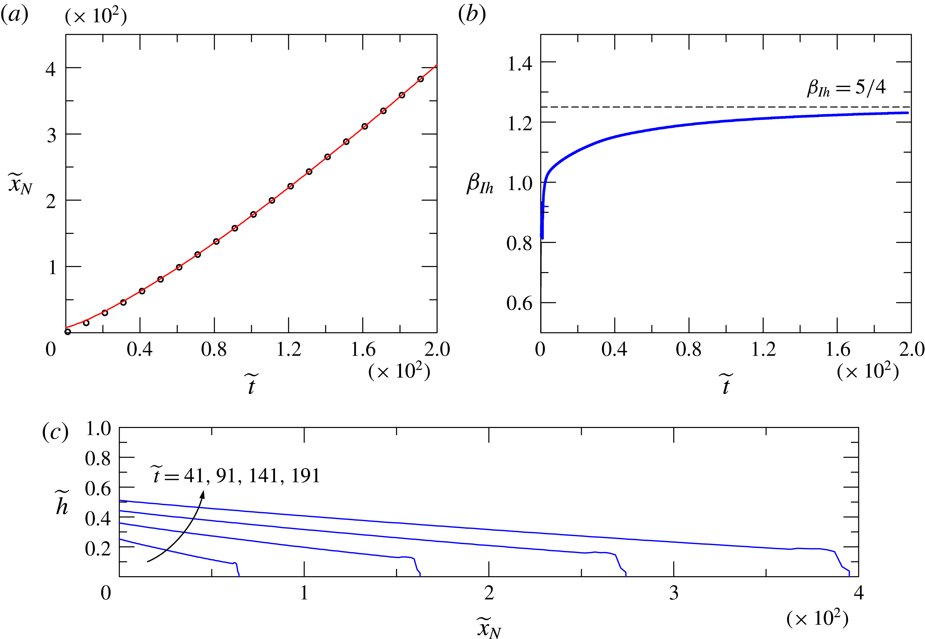
Numerical model results for a current advancing in a circular cross-section in the inertial–buoyancy regime in a linearly stratified ambient fluid (
 $S=1$
), with volume
 $\propto t^{9/4}$
(
 $\unicode[STIX]{x1D6FF}=9/4$
). (a) The time series of the front position
 $\widetilde{x}_{N}$
(symbols) and the interpolating function of the equation
 $\widetilde{x}_{N}\propto \widetilde{t}^{1.47}$
(continuous red curve); (b) the time series of the exponent
 $\unicode[STIX]{x1D6FD}_{Is}$
, with the dashed horizontal line representing the theoretical value
 $\unicode[STIX]{x1D6FD}_{Is}=3/2$
; (c) profiles of the current at different times.
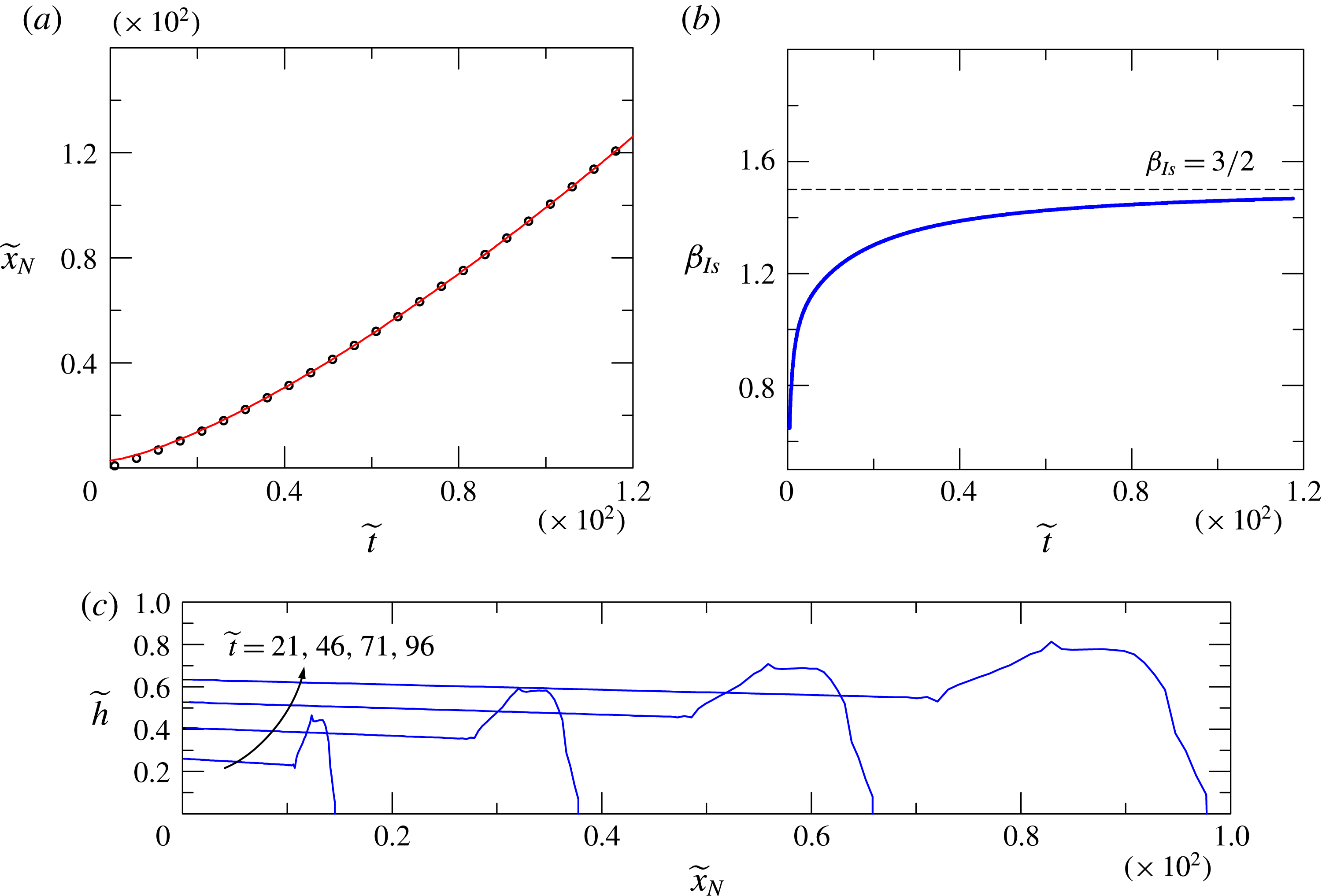
Appendix B. Viscous–buoyancy regime,
$S=0$

For a semicircular cross-section, the viscous–buoyancy force balance gives the following scales (see Longo et al. Reference Longo, Di Federico and Chiapponi2015a ):
 $$\begin{eqnarray}\displaystyle x_{\ast } & = & \displaystyle \left({\displaystyle \frac{q}{\sqrt{r}}}\right)^{2/(2\unicode[STIX]{x1D6FF}+5)}\left({\displaystyle \frac{\unicode[STIX]{x1D707}_{c}}{\unicode[STIX]{x1D70C}_{c}g^{\prime }}}\right)^{2\unicode[STIX]{x1D6FF}/(2\unicode[STIX]{x1D6FF}+5)},\end{eqnarray}$$
 $$\begin{eqnarray}\displaystyle t_{\ast } & = & \displaystyle \left({\displaystyle \frac{q}{\sqrt{r}}}\right)^{-2/(2\unicode[STIX]{x1D6FF}+5)}\left({\displaystyle \frac{\unicode[STIX]{x1D707}_{c}}{\unicode[STIX]{x1D70C}_{c}g^{\prime }}}\right)^{5/(2\unicode[STIX]{x1D6FF}+5)},\end{eqnarray}$$
where
 $g^{\prime }=(\unicode[STIX]{x1D70C}_{c}-\unicode[STIX]{x1D70C}_{0})/\unicode[STIX]{x1D70C}_{c}g$
is the reduced gravity, and the dimensional length of the current is
 $$\begin{eqnarray}x_{NV}=\unicode[STIX]{x1D702}_{N}(\unicode[STIX]{x1D6FF})\left({\displaystyle \frac{K_{C}}{2\sqrt{2}}}\right)^{1/2}\left({\displaystyle \frac{q}{\sqrt{r}}}\right)^{(2\unicode[STIX]{x1D6FD}_{Vh}+2)/(2\unicode[STIX]{x1D6FF}+5)}\left({\displaystyle \frac{\unicode[STIX]{x1D707}_{c}}{\unicode[STIX]{x1D70C}_{c}g^{\prime }}}\right)^{(2\unicode[STIX]{x1D6FF}-5\unicode[STIX]{x1D6FD}_{Vh})/(2\unicode[STIX]{x1D6FF}+5)}t^{\unicode[STIX]{x1D6FD}_{Vh}}.\end{eqnarray}$$
In critical condition (
 $\unicode[STIX]{x1D6FF}\equiv \unicode[STIX]{x1D6FF}_{ch}=2$
,
 $\unicode[STIX]{x1D6FD}_{Vh}\equiv \unicode[STIX]{x1D6FD}_{ch}=5/4$
), (B 3) yields
 $$\begin{eqnarray}x_{NV}=\left.\unicode[STIX]{x1D702}_{N}\right|_{\unicode[STIX]{x1D6FF}=2}\left({\displaystyle \frac{K_{C}}{2\sqrt{2}}}\right)^{1/2}\left({\displaystyle \frac{q}{\sqrt{r}}}\right)^{1/2}\left({\displaystyle \frac{\unicode[STIX]{x1D707}_{c}}{\unicode[STIX]{x1D70C}_{c}g^{\prime }}}\right)^{-1/4}t^{5/4},\end{eqnarray}$$
where
 $\left.\unicode[STIX]{x1D702}_{N}\right|_{\unicode[STIX]{x1D6FF}=2}\approx 1.4$
and
 $K_{C}=32\sqrt{2}/105\approx 0.43$
.
Appendix C. Inertial–buoyancy regime,
$S=0$

The dimensional expression of the length of the current in the inertial regime is computed by evaluating the length and time scales. The front condition reads as (dimensional)
 $$\begin{eqnarray}{\dot{x}}_{N}=Fr\sqrt{g^{\prime }h_{N}},\end{eqnarray}$$
which yields
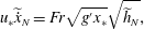 $$\begin{eqnarray}u_{\ast }\widetilde{{\dot{x}}}_{N}=Fr\sqrt{g^{\prime }x_{\ast }}\sqrt{\widetilde{h}_{N}},\end{eqnarray}$$
where the tilde indicates that the variable is dimensionless;
 $u_{\ast }$
and
 $x_{\ast }$
are the velocity and length scales respectively. The dimensional homogeneity requires
 $u_{\ast }=Fr\sqrt{g^{\prime }x_{\ast }}$
. The integral mass conservation is
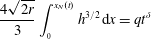 $$\begin{eqnarray}{\displaystyle \frac{4\sqrt{2r}}{3}}\int _{_{0}}^{x_{N}(t)}h^{3/2}\,\text{d}x=qt^{\unicode[STIX]{x1D6FF}}\end{eqnarray}$$
or
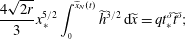 $$\begin{eqnarray}{\displaystyle \frac{4\sqrt{2r}}{3}}x_{\ast }^{5/2}\int _{_{0}}^{\widetilde{x}_{N}(t)}\widetilde{h}^{3/2}\,\text{d}\widetilde{x}=qt_{\ast }^{\unicode[STIX]{x1D6FF}}\widetilde{t}^{\unicode[STIX]{x1D6FF}};\end{eqnarray}$$
hence,
 $\sqrt{r}x_{\ast }^{5/2}=qt_{\ast }^{\unicode[STIX]{x1D6FF}}$
. By solving the system of equations (where
 $u_{\ast }=x_{\ast }/t_{\ast }$
), the scales are equal to
 $$\begin{eqnarray}\displaystyle & x_{\ast }=\left({\displaystyle \frac{q}{\sqrt{r}}}\right)^{2/(5-\unicode[STIX]{x1D6FF})}\left({\displaystyle \frac{1}{Fr\sqrt{g^{\prime }}}}\right)^{2\unicode[STIX]{x1D6FF}/(5-\unicode[STIX]{x1D6FF})}, & \displaystyle\end{eqnarray}$$
 $$\begin{eqnarray}\displaystyle & t_{\ast }=\left({\displaystyle \frac{q}{\sqrt{r}}}\right)^{1/(5-\unicode[STIX]{x1D6FF})}\left({\displaystyle \frac{1}{Fr\sqrt{g^{\prime }}}}\right)^{5/(5-\unicode[STIX]{x1D6FF})}. & \displaystyle\end{eqnarray}$$
Hence,
 $$\begin{eqnarray}x_{NI}\propto \left({\displaystyle \frac{q}{\sqrt{r}}}\right)^{(2-\unicode[STIX]{x1D6FD}_{Ih})/(5-\unicode[STIX]{x1D6FF})}\left({\displaystyle \frac{1}{Fr\sqrt{g^{\prime }}}}\right)^{(2\unicode[STIX]{x1D6FF}-5\unicode[STIX]{x1D6FD}_{Ih})/(5-\unicode[STIX]{x1D6FF})}t^{\unicode[STIX]{x1D6FD}_{Ih}}.\end{eqnarray}$$
In critical condition (
 $\unicode[STIX]{x1D6FF}\equiv \unicode[STIX]{x1D6FF}_{ch}=2$
,
 $\unicode[STIX]{x1D6FD}_{Ih}\equiv \unicode[STIX]{x1D6FD}_{ch}=5/4$
), (C 7) yields
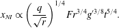 $$\begin{eqnarray}x_{NI}\propto \left({\displaystyle \frac{q}{\sqrt{r}}}\right)^{1/4}Fr^{3/4}{g^{\prime }}^{3/8}t^{5/4}.\end{eqnarray}$$
Appendix D. Viscous–buoyancy regime,
$S=1$

Use of (2.5) gives
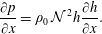 $$\begin{eqnarray}{\displaystyle \frac{\unicode[STIX]{x2202}p}{\unicode[STIX]{x2202}x}}=\unicode[STIX]{x1D70C}_{0}\,{\mathcal{N}}^{\,2}h{\displaystyle \frac{\unicode[STIX]{x2202}h}{\unicode[STIX]{x2202}x}}.\end{eqnarray}$$
For the viscous controlled regime, the force balance
 $F_{V}\sim F_{B}$
is required. In a circular cross-section approximated by a parabola (
 $\unicode[STIX]{x1D6FC}=1/2$
), the dominant shear stress acts along the vertical; hence,
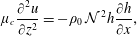 $$\begin{eqnarray}\unicode[STIX]{x1D707}_{c}{\displaystyle \frac{\unicode[STIX]{x2202}^{2}u}{\unicode[STIX]{x2202}z^{2}}}=-\unicode[STIX]{x1D70C}_{0}\,{\mathcal{N}}^{\,2}h{\displaystyle \frac{\unicode[STIX]{x2202}h}{\unicode[STIX]{x2202}x}},\end{eqnarray}$$
which in turn allows the computation of the velocity
 $u(x,y,z)$
by imposing the boundary conditions at the wall of the cross-section and at the interface with the ambient fluid.
Integration of the velocity over the cross-section of the current gives the volume discharge as
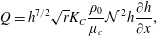 $$\begin{eqnarray}Q=h^{7/2}\sqrt{r}K_{C}{\displaystyle \frac{\unicode[STIX]{x1D70C}_{0}}{\unicode[STIX]{x1D707}_{c}}}{\mathcal{N}}^{\,2}h{\displaystyle \frac{\unicode[STIX]{x2202}h}{\unicode[STIX]{x2202}x}},\end{eqnarray}$$
where
 $K_{C}=32\sqrt{2}/105$
is a coefficient, with the subscript standing for ‘circular’. The differential form of the mass conservation reads as
 $$\begin{eqnarray}h^{1/2}{\displaystyle \frac{\unicode[STIX]{x2202}h}{\unicode[STIX]{x2202}t}}-{\displaystyle \frac{\sqrt{2}K_{C}}{4}}{\displaystyle \frac{\unicode[STIX]{x1D70C}_{0}\,{\mathcal{N}}^{\,2}}{\unicode[STIX]{x1D707}_{c}}}{\displaystyle \frac{\unicode[STIX]{x2202}}{\unicode[STIX]{x2202}x}}\left(h^{9/2}{\displaystyle \frac{\unicode[STIX]{x2202}h}{\unicode[STIX]{x2202}x}}\right)=0,\end{eqnarray}$$
which, by introducing the length and the time scales, can be written as
 $$\begin{eqnarray}{\displaystyle \frac{x_{\ast }^{3/2}}{t_{\ast }}}\widetilde{h}^{1/2}{\displaystyle \frac{\unicode[STIX]{x2202}\widetilde{h}}{\unicode[STIX]{x2202}\widetilde{t}}}-{\displaystyle \frac{\sqrt{2}K_{C}}{4}}{\displaystyle \frac{\unicode[STIX]{x1D70C}_{0}\,{\mathcal{N}}^{\,2}}{\unicode[STIX]{x1D707}_{c}}}x_{\ast }^{7/2}{\displaystyle \frac{\unicode[STIX]{x2202}}{\unicode[STIX]{x2202}\widetilde{x}}}\left(\widetilde{h}^{9/2}{\displaystyle \frac{\unicode[STIX]{x2202}\widetilde{h}}{\unicode[STIX]{x2202}\widetilde{x}}}\right)=0.\end{eqnarray}$$
The integral mass conservation is again (C 4).
The corresponding length and time scales are computed from (D 5) and (C 4) as
 $$\begin{eqnarray}\displaystyle x_{\ast } & = & \displaystyle \left({\displaystyle \frac{q}{\sqrt{r}}}\right)^{2/(4\unicode[STIX]{x1D6FF}+5)}\left({\displaystyle \frac{\unicode[STIX]{x1D707}_{c}}{\unicode[STIX]{x1D70C}_{0}\,{\mathcal{N}}^{\,2}}}\right)^{2\unicode[STIX]{x1D6FF}/(4\unicode[STIX]{x1D6FF}+5)},\end{eqnarray}$$
 $$\begin{eqnarray}\displaystyle t_{\ast } & = & \displaystyle \left({\displaystyle \frac{q}{\sqrt{r}}}\right)^{-4/(4\unicode[STIX]{x1D6FF}+5)}\left({\displaystyle \frac{\unicode[STIX]{x1D707}_{c}}{\unicode[STIX]{x1D70C}_{0}\,{\mathcal{N}}^{\,2}}}\right)^{5/(4\unicode[STIX]{x1D6FF}+5)}.\end{eqnarray}$$
The system of equations (D 5)–(C 4) then becomes, in dimensionless form,
 $$\begin{eqnarray}\widetilde{h}^{1/2}{\displaystyle \frac{\unicode[STIX]{x2202}\widetilde{h}}{\unicode[STIX]{x2202}\widetilde{t}}}-{\displaystyle \frac{\unicode[STIX]{x2202}}{\unicode[STIX]{x2202}\widetilde{x}}}\left(\widetilde{h}^{9/2}{\displaystyle \frac{\unicode[STIX]{x2202}\widetilde{h}}{\unicode[STIX]{x2202}\widetilde{x}}}\right)=0,\quad {\displaystyle \frac{4\sqrt{2}}{3}}\int _{0}^{\widetilde{x}_{N}(t)}\widetilde{h}^{3/2}\,\text{d}\widetilde{x}=\widetilde{t}^{\,\unicode[STIX]{x1D6FF}},\end{eqnarray}$$
and admits a self-similar solution expressed as
 $$\begin{eqnarray}\widetilde{h}=\unicode[STIX]{x1D702}_{N}^{1/2}\,\widetilde{t}^{\,(2\unicode[STIX]{x1D6FF}-1)/7}f(\unicode[STIX]{x1D702}),\quad \unicode[STIX]{x1D702}=\left({\displaystyle \frac{2\sqrt{2}}{K_{C}}}\right)^{1/2}\widetilde{x}\,\widetilde{t}^{\,-(8\unicode[STIX]{x1D6FF}+3)/14},\end{eqnarray}$$
where
 $$\begin{eqnarray}\unicode[STIX]{x1D702}_{N}=\unicode[STIX]{x1D702}_{N}(\unicode[STIX]{x1D6FF})=\left[{\displaystyle \frac{4\sqrt{2}}{3}}\left({\displaystyle \frac{K_{C}}{2\sqrt{2}}}\right)^{1/2}\int _{0}^{1}f^{3/2}\,\text{d}\unicode[STIX]{x1D701}\right]^{-4/7}\,\unicode[STIX]{x1D701}={\displaystyle \frac{\unicode[STIX]{x1D702}}{\unicode[STIX]{x1D702}_{N}}}.\end{eqnarray}$$
The length of the current is then
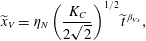 $$\begin{eqnarray}\widetilde{x}_{V}=\unicode[STIX]{x1D702}_{N}\left({\displaystyle \frac{K_{C}}{2\sqrt{2}}}\right)^{1/2}\widetilde{t}^{\,\unicode[STIX]{x1D6FD}_{Vs}},\end{eqnarray}$$
where
 $\unicode[STIX]{x1D6FD}_{Vs}=(8\unicode[STIX]{x1D6FF}+3)/14$
. Finally, the (dimensional) length of the current in the viscous regime for
 $S=1$
is derived as
 $$\begin{eqnarray}x_{NV}=\unicode[STIX]{x1D702}_{N}\left({\displaystyle \frac{K_{C}}{2\sqrt{2}}}\right)^{1/2}\left({\displaystyle \frac{q}{\sqrt{r}}}\right)^{(2+4\unicode[STIX]{x1D6FD}_{Vs})/(5+4\unicode[STIX]{x1D6FF})}\left({\displaystyle \frac{\unicode[STIX]{x1D707}_{c}}{\unicode[STIX]{x1D70C}_{0}\,{\mathcal{N}}^{\,2}}}\right)^{(2\unicode[STIX]{x1D6FF}-5\unicode[STIX]{x1D6FD}_{VS})/(5+4\unicode[STIX]{x1D6FF})}t^{\unicode[STIX]{x1D6FD}_{Vs}}.\end{eqnarray}$$
In critical condition (
 $\unicode[STIX]{x1D6FD}_{Vs}\equiv \unicode[STIX]{x1D6FD}_{cs}=3/2$
,
 $\unicode[STIX]{x1D6FF}\equiv \unicode[STIX]{x1D6FF}_{cs}=9/4$
), (D 12) yields
 $$\begin{eqnarray}x_{NV}=\left.\unicode[STIX]{x1D702}_{N}\right|_{\unicode[STIX]{x1D6FF}=9/4}\left({\displaystyle \frac{K_{C}}{2\sqrt{2}}}\right)^{1/2}\left({\displaystyle \frac{q}{\sqrt{r}}}\right)^{4/7}\left({\displaystyle \frac{\unicode[STIX]{x1D707}_{c}}{\unicode[STIX]{x1D70C}_{0}\,{\mathcal{N}}^{\,2}}}\right)^{-3/14}t^{3/2},\end{eqnarray}$$
with
 $\left.\unicode[STIX]{x1D702}_{N}\right|_{\unicode[STIX]{x1D6FF}=9/4}\approx 1.056$
.
Appendix E. Inertial–buoyancy regime,
$S=1$

The inertial–buoyancy balance is
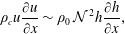 $$\begin{eqnarray}\unicode[STIX]{x1D70C}_{c}u{\displaystyle \frac{\unicode[STIX]{x2202}u}{\unicode[STIX]{x2202}x}}\sim \unicode[STIX]{x1D70C}_{0}\,{\mathcal{N}}^{\,2}h{\displaystyle \frac{\unicode[STIX]{x2202}h}{\unicode[STIX]{x2202}x}},\end{eqnarray}$$
which becomes, in dimensionless form,
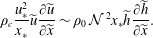 $$\begin{eqnarray}\unicode[STIX]{x1D70C}_{c}{\displaystyle \frac{u_{\ast }^{2}}{x_{\ast }}}\widetilde{u}{\displaystyle \frac{\unicode[STIX]{x2202}\widetilde{u}}{\unicode[STIX]{x2202}\widetilde{x}}}\sim \unicode[STIX]{x1D70C}_{0}\,{\mathcal{N}}^{\,2}x_{\ast }\widetilde{h}{\displaystyle \frac{\unicode[STIX]{x2202}\widetilde{h}}{\unicode[STIX]{x2202}\widetilde{x}}}.\end{eqnarray}$$
The continuity equation is again (C 4),
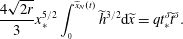 $$\begin{eqnarray}{\displaystyle \frac{4\sqrt{2r}}{3}}x_{\ast }^{5/2}\int _{_{0}}^{\widetilde{x}_{N}(t)}\widetilde{h}^{3/2}\text{d}\widetilde{x}=qt_{\ast }^{\unicode[STIX]{x1D6FF}}\widetilde{t}^{\unicode[STIX]{x1D6FF}}.\end{eqnarray}$$
In the Boussinesq approximation (
 $\unicode[STIX]{x1D70C}_{0}/\unicode[STIX]{x1D70C}_{c}\approx 1$
), equations (C 4)–(E 2) yield the characteristic length and time scales as follows:
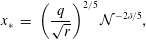 $$\begin{eqnarray}\displaystyle x_{\ast } & = & \displaystyle \left({\displaystyle \frac{q}{\sqrt{r}}}\right)^{2/5}{\mathcal{N}}^{-2\unicode[STIX]{x1D6FF}/5},\end{eqnarray}$$
 $$\begin{eqnarray}\displaystyle t_{\ast } & = & \displaystyle {\mathcal{N}}^{-1}.\end{eqnarray}$$
The (dimensional) length of the current in the inertial–buoyancy regime is then
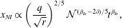 $$\begin{eqnarray}x_{NI}\propto \left({\displaystyle \frac{q}{\sqrt{r}}}\right)^{2/5}{\mathcal{N}}^{(\unicode[STIX]{x1D6FD}_{Is}-2\unicode[STIX]{x1D6FF})/5}t^{\unicode[STIX]{x1D6FD}_{Is}},\end{eqnarray}$$
where
 $\unicode[STIX]{x1D6FD}_{Is}=(3+2\unicode[STIX]{x1D6FF})/5$
. In critical condition (
 $\unicode[STIX]{x1D6FD}_{Is}\equiv \unicode[STIX]{x1D6FD}_{cs}=3/2$
and
 $\unicode[STIX]{x1D6FF}\equiv \unicode[STIX]{x1D6FF}_{cs}=9/4$
), (E 6) reads as
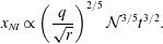 $$\begin{eqnarray}x_{NI}\propto \left({\displaystyle \frac{q}{\sqrt{r}}}\right)^{2/5}{\mathcal{N}}^{3/5}t^{3/2}.\end{eqnarray}$$



